Synchronization in a multilevel network using the Hamilton-Jacobi-Bellman (HJB) technique
Abstract
This paper presents the optimal control and synchronization problem of a multilevel network of Rössler chaotic oscillators. Using the Hamilton-Jacobi-Bellman (HJB) technique, the optimal control law with three-state variables feedback is designed such that the trajectories of all the Rössler oscillators in the network are optimally synchronized in each level. Furthermore, we provide numerical simulations to demonstrate the effectiveness of the proposed approach for the cases of one and three networks. A perfect correlation between the MATLAB and the PSPICE results was obtained, thus allowing the experimental validation of our designed controller and shows the effectiveness of the theoretical results.
I Introduction
The history of the synchronization of dynamical systems goes back to Christiaan Huygens in 1665 pikovsky2003synchronization and, in the past three decades, it has become a subject of intensive research due to their various domains of applications in fields like mathematics, physics, biology, economics, technology, engineering mosekilde2002chaotic; kose2003does; pikovsky2003synchronization; acebron2005kuramoto; chopra2005synchronization; dorfler2013synchronization. This phenomenon exists in the case of two coupled systems as well as a network pikovsky2003synchronization; lu2002chaos; fujiwara2011synchronization. In recent decades, several works based on the study of synchronization in complex networks have focused on the problem of orienting the network towards a collective state shared by all the units, but for the most part considering the coupling coefficient as the control parameter used to achieve this dynamic fujiwara2011synchronization; reff7; relaysynchro; ref9.
After an initial period of characterization of the complex networks in terms of local and global statistical properties, attention was turned to the dynamics of their interacting units. A widely studied example of such behavior is synchronization of coupled oscillators arranged into complex networks fujiwara2011synchronization. Synchronization can found applications in communication systems, system’s security and secrecy or cryptographyguo2021partial; banerjee2010chaos.
The investigations on the behavior of the network cooperative systems (or multi-agent systems) has received extensive attention, mainly due to its widespread applications such as mobile robots, spacecraft, networked autonomous team, sensor networks, etc. ren2005survey; olfati2007consensus; zhang2011optimal. In all these applications, whatever the field, the main idea is control. Based on the literature of the control, a wide variety of approaches have been developed to control the behaviour of the systems in a network. Several methods have been proposed to achieve chaos synchronization such as impulsive control, adaptive control, time-delay feedback approach, active control, sliding mode, pinning control, compound synchronization, nonlinear control, al2009anti; el2009synchronization; naderi2016exponential; naderi2016optimal; rigatos2021nonlinear; rigatos2019synchronization; shi2022guaranteed; rigatos2022nonlinear etc. Most of the above methods were used to synchronize two identical chaotic systems using adaptive methods.
To control a system is to be able to perform the appropriate modification on its inputs in order to place the outputs in a desired state. Most studies conducted in complex systems and particularly in the control of network dynamics use linear (usually diffusive) coupling models to study network dynamics pikovsky2003synchronization; lu2002chaos; reff7; relaysynchro; ref9; njougouo2020dynamics. This method is limited because it takes too long to achieve synchronization thus rendering simulations practically useless.
To solve this problem, we propose to build an optimal controller in the case of a network of chaotic oscillators that will not only reduce the transient phase to achieve the desired behaviour but it also reduces considerably the simulation time. It is important to mention that this work completes the work of Rafikov and Balthazarrafikov2008 who initially presented the synchronization of two Rössler chaotic systems based on the HJB techniques.
The structure of the article is as follows: In Sect.II, the control of the dynamics of one network (sometimes called patch) of 50 Rössler chaotic oscillators based on the formulation of the problem is introduced a theorem illustrating how to design the controllers is proven also in this section. In Sect. III, the HJB technique presented in Sect.II is extended to three networks of 50 Rössler chaotic oscillators. Then, in Sec. IV we illustrate the implementation of the technique using electronic circuits for a small number of oscillators.
II Synchronization of a network of Rössler chaotic oscillators
The purpose of this section is to introduce a development optimal control law to resolve for the optimal synchronization of Rössler chaotic oscillators. The optimal control law is obtained using the Hamilton-Jacobi-Bellman (HJB) techniquerafikov2008; liu2018design.
II.1 Problem Formulation
First we present the model of a single network. Fig.1 shows the topology of connections between the nodes of the network.

Let us consider the well-known Rössler system rossler1979continuous; njougouo2020dynamics as the node dynamics with the following mathematical description Eq.1.
| (1) |
where , and .
The system has a zero bounded volume, globally attracting set moon1987chaotic; el2006optimal. Hence, for all time , the state trajectories are globally bounded and continuously differentiable with respect to time . Thereby, positive constants for all the nodes of the network exist such that:
| (2) |
where is the norm of the system identified by the index , is maximum constant for the node and is the maximum constant for all nodes in the network.
Our goal is to develop an optimal control to guarantee the complete synchronization of all systems in the network. We assume that the controlled model is defined by Eq.3.
| (3) |
where : represents the self-dynamics of node (see Eq.1) of the network and . Taking into account the controller the dynamics of the network becomes:
| (4) |
As mentioned previously, the goal is to design an appropriate optimal controller ( and ) such that for any initial condition, we have:
| (5) |
where represents the Euclidean norm and the error between system and system defined by . Therefore, the dynamical system error between node and node is calculated as follows:
| (6) |
Clearly, the optimal synchronization problem is now replaced by the equivalent problem of optimally stabilizing the error system Eq.6 using a suitable choice of the controllers and . In order to generalize Rafikov and Balthazar’s workrafikov2008 to apply for a network we prove that:
Theorem II.1
The controlled Rössler chaotic oscillators presented by Eq.4 will asymptotically synchronize provided the optimal controller found minimizes the performance functional defined by Eq.7.
| (7) |
Let be the feedback controllers that minimize the above integral measure with , and being the weight of the links which satisfy the relationship .
The dynamical system error Eq.6 converge to equilibrium ( and ).
Proof: Let us assume that the minimum of Eq.7 is obtained with }. So, we have:
| (8) |
The function may be treated as the Lyapunov function candidate.
Using the Hamilton-Jacobi-Bellman technique, we find the optimal controller such that the systems Eq.6 is stabilized to equilibrium points and the integral Eq.7 is minimum. Therefore we have:
| (10) |
The Minimization of the Eq.10 with respect to gives the following optimal controllers:
| (11) |
with and
Replacing Eq.11 into Eq.10 we obtain the following Equation:
| (12) |
Now considering
| (13) |
The Hamilton-Jacobi-Bellman relation described by Eq.12 is satisfied. Thereby the optimal controllers can be derived as follows:
| (14) |
where the constants and are positive. Differentiating the function in Eq.13 along the optimal trajectories we have:
| (15) |
Therefore, we can select as a Lyaponuv function. According to khalil2002nonlinear; naderi2016optimal, this shows the solutions of the system Eq.6 are asymptotically stable in the Lyapunov sense via optimal control.
II.2 Numerical simulation of the optimal synchronization in a single network
In order to demonstrate the effectiveness and validity of the proposed results in an optimal controller in the case of the network (patch) described in Eq.4, we present and discuss the numerical results. We use MATLAB software with fourth order Runge-Kutta integration method for numerical resolution of the non-linear differential equations.
We consider a network constituted by Rössler chaotic oscillators with the optimal controllers obtained in Theorem 2.1. According to Reftang2019master the synchronization error of the whole network can be calculated using the relation given by:
| (16) |
In Fig.2 the we present the dynamics of the systems in the network, without control.

In Fig.2(a) we can observe the dynamics of each oscillator of the network and we conclude that synchronization does not exist here. This situation is confirmed in Fig.2(b) by non-zero synchronization error in this network. According to the literature, synchronization between chaotic oscillators is due to the presence of the coupling or control between these systems. Therefore, the results presented in Fig.2 are normal because in the absence of any type of interaction or control the existence of synchronization is a random fact.
Now we proceed to demonstrate the effectiveness of the optimal control obtained in Theorem 2.1. In Fig.3(a) we show the time series of synchronized elements for a network of Rössler chaotic oscillators for the constant parameters in the optimal controller: and with . This chaotic synchronization is confirmed by the synchronization error plotted in Fig.3(b). Therefore, it comes that the sum system is asymptotically stable.


Based on these results, it appears that this controller designed in Eq.14 leads the systems of the network in a synchronous state with finite time. So, it is important to evaluate the impact of these constant parameters appearing in optimal controllers on the time of synchronization of the systems of the network. Therefore, we present in Fig.3(c) the synchronization errors of the network for three pairs of constant parameter values in the optimal controller where and corresponds to in red, and corresponds to in cian and and corresponds to in black. This figure leads us to conclude that, when the constant parameter increases the time required to reach synchronization decreases.
III Dynamics of a multi network with intra network optimal control and diffusive coupling between networks
In this section, we consider a model formed by three networks(see Fig.4). Each network is made up of homogeneous (identical) systems but subject to different initial conditions. The main objective here is to show that the controller obtained previously remains optimal for intra-layer synchronization and that the control of the model towards a desired behaviour comes down to the inter-layer coupling chosen diffusive.
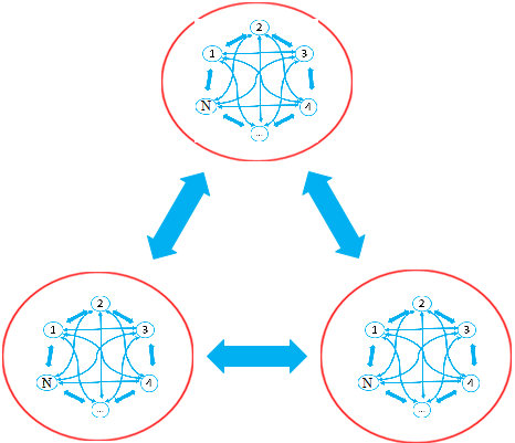
In this representation, the mathematical description of each network is given as follow:
First network
| (17) |
Second network
| (18) |
Third network
| (19) |
where , and are the systems parameter and , where is the number of elements in a single network. The states vector , and represent the first, second and third patch, respectively. , and are the intra-network optimal controllers of the first, second and third network respectively.
It is important to mention that these controllers are obtained without any inter-network connection. Therefore, based on the previous section, the objective in all networks is the same, and the objective function for all these three networks is also the same. Following Theorem 2.1, the optimal controllers in each network will be defined as follows:
First network
| (20) |
with , .
Second network
| (21) |
with , .
Third network
| (22) |
with ,
Using the optimal controllers presented in Eqs.20, 21, 22 and without inter-network coupling (), we show in Fig.5 the dynamics of each of the previously defined network. The Figs.5(a,b and c) show the time series of the first, second and third network respectively and the Figs.5(d,e and f) present the synchronization error in a much smaller times interval for a good appreciation. These figures give a good indication of the validity of the proposed control.

Turning on the interlayer coupling in a multi-network modifies some parameters in the corresponding error . The calculations although simple are cumbersome due to the indexes involved therefore we test the performance of the proposed optimal control scheme through experimental simulations. We have left to the appendix A to show that the stability of the synchronization of the whole network depends on the intra-layer synchronization. This demonstration shows that the synchronization of the whole network is conditioned by the intra-layer synchronization. The simulations show that under the proposed control method, synchronization is achieved between all systems of all networks. We investigate simultaneously the impact of the coupling weight of the control and the inter-network coupling, and we obtain three different dynamics for the whole multilevel network which we show in Fig.6. These results are obtained under the following considerations: the weight in the second network is ( and ) and the inter-network coupling is in the first and the third network. Thus, varying simultaneously the weights in the first and third networks as well as the inter network coupling in the second network, we obtain four domains:


first domain (green), where complete synchronization is achieved for all elements of the multilevel system as can be noted in Fig.7(a,b). In Figs.7 we represent the phase of the oscillators, calculated using the Hilbert transform and expressed in degrees defined as in Refrosenblum1996phase; pikovsky1997phase as well as a three dimensional representation of the oscillator state, to show the dynamics of the single oscillators in each of the phases shown in Fig.6. In (Fig.7(a,b)) the oscillators of these three networks form a single cluster. The second domain (red) indicates the region where the first and third networks synchronize. The particularity of this domain lies in the formation of two clusters as presented by Fig.7(c and d) and all the three networks are internally completely synchronized. The black domain has practically the same properties as the previous red domain except that the second network shows a disordered state. This leaves the entire network to behave like a chimera as in Fig.7(e,f). The last domain (blue) represents the parameter region when complete synchronization is not possible while each single network is completely synchronized at different phase values, as shown in Fig.7(g,h). The investigation of the stability of the synchronization in the whole network shows that this synchronization of the whole network is possible only if the systems synchronize first in the different layers as shown in appendix A.
These studies show that the network can exhibit several behaviours depending on the parameters chosen.


IV Circuit implementation
In this section we focus on implementing the networks as circuits which can serve as a powerful tool to qualitatively describe quickly and cheaply the features that we want to demonstrate and therefore, suggest devices for real experiments. For this implementation, we initially consider the case of one network with three Rössler oscillators and the study will extended to the case of three networks as in Sec.III. In order to better appreciate the experimental results that will be given later, we have redone the studies presented in Fig.6 but, now considering 3 oscillators per network (i.e. 9 oscillators for the whole network). The results of this study are presented in Fig.8 and like those of Fig.6 they show the dynamics of the whole network for N=3 oscillators per network.


This Fig.8 reproduces exactly the same dynamics as those observed in Fig.6 for the same range of variation of the weight (which allows to control the intra-network dynamics) and the inter-network coupling (which controls the inter-network dynamics). The only difference is in the number of oscillators per patch.


Based on Fig.8, we illustrate in Fig.9 different behaviours such as: synchronization of these three networks (see Fig.9(a,b)) presenting one cluster formation for the whole network. We can also have synchronization between the first and the third network as it appears in Fig.9(c,d), where the whole network presents two clusters. As illustrated in Fig.7(e,f), the same result is reproduced for the case of three systems per network (see Fig.9(e,f)). In the same vein we can mention the possibility of having three clusters in the network, it only takes to make the inter-network couplings weak or null as recommended in Fig.8 and where the snapshot is given in Fig.9(g,h)).
In Fig. 9 we represent the dynamics of the phases as well as the temporal dynamics of the whole network. The results presented in a way to be easily compared with Fig.7 show that the experimental results follow closely those predicted by theory.
The goal of the next step is to design a suitable Pspice circuit simulator to investigate the systems described by Eqs.4, 17, 18 and 19 with their controllers (Eqs.14, 20, 21 and 22 respectively) in order to validate and support our theoretical results. But, the numerical solutions of the basic Rössler defined by Eq.1 without coupling term cannot be implemented using general circuit components due to the high amplitude of the signals that can destroy these components. In practice, it often needs to be varied to make proper adjustments to these variables njougouo2020effects. Thus, the amplitude range of each variable value varies greatly. The working voltage range of electronic components is generally between and in practical electronic circuits. Thereby, implementing a synchronization strategy implies taking into consideration the constraints by saturation coming from the electronic components of the circuit femat2009accounting. The reason for this could be the high amplitudes (at least for a certain transient time) of the coupling functions that sometimes are really higher than the state variables of the systems femat2009accounting; louodop2014adaptive. Therefore, to implement the electronic circuit of our systems, we need to scale the variables of the systems. Thus, for the electrical equations we choose (with =1,2,…,N the index of the systems) as the state variables of the systems of the network of Rössler oscillators.
In order to avoid a very cumbersome presentation due to the amount of components of the circuit, we present in Fig.10 only the circuit of one Rössler chaotic oscillator with and being the polarization voltages of the operational amplifiers used. In this circuit, , and denote the inputs of the first, second and third variable of the oscillator and , and the outputs. Based on the previous transformation and using Kirchoff and Millmann laws we present in Eqs.23 the circuit equations of the model presented previously in Eq.4. The electronic circuit of the controller designed by Eq.14 is given in Fig.11 and their circuit equations by Eq.24. For this implementation, the number of oscillators per network is N=3.


| (23) |
With:
| (24) |
where and . After some mathematical calculations we arrive at the following choice of component values: , , , , , . The values of the components used in Eq.24 depend on the weight used previously: , and .


The investigations of the effect of the weight on the transition to synchronization (presented in Fig.3) are also checked using electronic circuits (see Fig.10 for the electronic circuit of the oscillator in one network and Fig.11 for the electronic circuit modeling the controller between the and oscillator. The simulation with the Pspice software of the whole circuit in the case of one network leads us to the results presented in Fig.12 for two values of the weight. This result is captured directly from the graphical interface of the software Pspice for authenticity. In Fig.12(a) where and the computation of the values of the components of Fig.11 leads to the following values: , , , and . In Fig.12(b) we have , , , and for and . This result shows not only the synchronization of the three circuits used in this network but also we can observe that, when we increase the value of the weight the transient time to obtain synchronization is reduced. Therefore, it confirm the effectiveness of the proposed control and the previous result (Fig.3(c)) obtained in MATLAB.
For the case of three networks as presented in Fig.4, we have decided to simplify the equations and have considered the general form given by:
| (25) |
where and are respectively the optimal controllers obtained in each network and the coupling strength between the networks. So the electrical equations of each network can be expressed as follow:
| (26) |
Eq.26 is obtained according to the elements (components) of Fig.13 while respecting the values of the parameters given previously.

This Fig.13 shows the circuit of the whole network of 9 Rössler chaotic oscillators. This global network as mentioned above is formed by 3 oscillators per sub-network. Thus on this Figure, the boxes marked Network1, Network2 and Network3 represent respectively the first, the second and the third network where the control laws and the systems are those given in Fig.10 and 11. The diffusive couplings between the patches are represented in Fig.13. The terminals , and represent the inputs of the three systems in each patch (network) and the terminals , and the corresponding outputs in each patch. The values of the resistances marked in this Fig.13 correspond to used previously in MATLAB simulation. After simulation in Pspice, we show in Fig.14 the time series of the whole network constituted by 3N oscillators.


In Fig.14(a) we present the time series of the first oscillator of each network for , and . And in Fig.14(b) we show the time series of the nine oscillators of the whole network. Based on these results we can confirm the effectiveness of our control in the case of three networks.


To further investigate and validate the experimental results, studies have been made using the circuit shown in Fig.13. The results of these studies, which are presented in Fig.15, allowed us to show the existence of the phenomena observed theoretically in MATLAB. Among these phenomena we have the synchronization of the three networks (see Fig.15(a,b)), the synchronization between the network 1 and 3 (see Fig.15(c,d)) and the formation of three clusters (Fig.15(e,f)).
V Conclusion
This paper presents a theoretical and experimental study (study performed under MATLAB and PSPICE) on achieving optimal synchronization for a multi-network network of Rössler chaotic oscillators. An optimal controller was designed in this study firstly for the synchronization of a network (or a network) of 50 Rössler chaotic oscillators and secondly for the synchronization of three networks of 50 Rössler chaotic oscillators. The designed optimal control law satisfied Lyapunov’s stability theorem and the HJB technique. It also shows under simulation that, the control method we developed can guarantee a chaotic state for all the oscillators of the network at the synchronization. Using this control method, it also demonstrates the possibility to obtain complete synchronization for the three networks, cluster formation or a semblance of chimera state for the global network. Electronic circuits also show the effectiveness of the proposed method.
VI Data Availability Statement
The data that supports the findings of this study are available within this article.
Acknowledgements
T.N. thanks the University of Namur for the financial support. HAC thanks ICTP-SAIFR and FAPESP grant 2016/01343-7 for partial support. P.L. acknowledges support by the FAPESP Grant No.2014/13272-1.
Appendix A Stability of the all network synchronization
Let consider the simultaneous synchronization error, from all the nodes in the multilevel network consisting of the coupled three layers, expressed as , and the intra-layer couplings described by the following expressions:
| (27) |
For simplicity, we chose for and we consider are identical. Thus, the coupling between layers becomes:
and the intralayer coupling becomes:
| (28) |
| (29) |
Considering the previous relations, we obtain the following error system:
| (30) |
The problem now is to prove the stability of the entire connected layers basing ourselves on the error system Eq.30. To do so, let select the following Lyapunov function as given by Eq.31.
| (31) |
Its time derivative is expressed by the following Eq.32
| (32) |
Considering that:
, then
Thus, relation Eq.32 becomes:
| (33) |
| (34) |
| (35) |
where
| (36) |
| (37) |
From here, it comes out that the time derivative of the Lyapunov function in Eq.37 is negative if the nodes in each layer synchronize namely if for all and . Thus,
| (38) |
| (39) |
Integrating the preview equation from zero to t yields,
| (40) |
As goes to infinity, the above integral is always less than or equal to . Since is positive and finite, exists and is finite. Thus, according to the Barbalat Lemmaedwards2000sliding, one obtains:
| (41) |
Which implies that . This achieves the proof.
References
- (1) Juan A Acebrón, Luis L Bonilla, Conrad J Pérez Vicente, Félix Ritort, and Renato Spigler. The kuramoto model: A simple paradigm for synchronization phenomena. Reviews of modern physics, 77(1):137, 2005.
- (2) M Mossa Al-Sawalha and M Salmi Md Noorani. Anti-synchronization of two hyperchaotic systems via nonlinear control. Communications in Nonlinear Science and Numerical Simulation, 14(8):3402–3411, 2009.
- (3) Santo Banerjee. Chaos synchronization and cryptography for secure communications: applications for encryption. IGI global, 2010.
- (4) Nikhil Chopra and Mark W Spong. On synchronization of kuramoto oscillators. In Proceedings of the 44th IEEE Conference on Decision and Control, pages 3916–3922. IEEE, 2005.
- (5) Florian Dörfler, Michael Chertkov, and Francesco Bullo. Synchronization in complex oscillator networks and smart grids. Proceedings of the National Academy of Sciences, 110(6):2005–2010, 2013.
- (6) Christopher Edwards, Sarah K Spurgeon, and Ron J Patton. Sliding mode observers for fault detection and isolation. Automatica, 36(4):541–553, 2000.
- (7) MM El-Dessoky. Synchronization and anti-synchronization of a hyperchaotic chen system. Chaos, Solitons & Fractals, 39(4):1790–1797, 2009.
- (8) Awad El-Gohary and Ammar Sarhan. Optimal control and synchronization of lorenz system with complete unknown parameters. Chaos, Solitons & Fractals, 30(5):1122–1132, 2006.
- (9) Ricardo Femat, C Jiménez, Samuel Bowong, and Gualberto Solís-Perales. Accounting the control effort to improve chaos suppression via robust adaptive feedback. International Journal of Modelling, Identification and Control, 6(2):147–155, 2009.
- (10) Naoya Fujiwara, Jürgen Kurths, and Albert Díaz-Guilera. Synchronization in networks of mobile oscillators. Physical Review E, 83(2):025101, 2011.
- (11) Rongwei Guo and Yi Qi. Partial anti-synchronization in a class of chaotic and hyper-chaotic systems. IEEE Access, 9:46303–46312, 2021.
- (12) Hassan K Khalil and Jessy W Grizzle. Nonlinear systems, volume 3. Prentice hall Upper Saddle River, NJ, 2002.
- (13) M Ayhan Kose, Eswar S Prasad, and Marco E Terrones. How does globalization affect the synchronization of business cycles? American Economic Review, 93(2):57–62, 2003.
- (14) I Leyva, I Sendiña-Nadal, R Sevilla-Escoboza, VP Vera-Avila, P Chholak, and S Boccaletti. Relay synchronization in multiplex networks. Sci. Rep., 8(1):1–11, 2018.
- (15) Ziqian Liu. Design of nonlinear optimal control for chaotic synchronization of coupled stochastic neural networks via hamilton–jacobi–bellman equation. Neural Networks, 99:166–177, 2018.
- (16) Patrick Louodop, Hilaire Fotsin, Samuel Bowong, and A Soup Tewa Kammogne. Adaptive time-delay synchronization of chaotic systems with uncertainties using a nonlinear feedback coupling. Journal of Vibration and Control, 20(6):815–826, 2014.
- (17) Jinhu Lü, Tianshou Zhou, and Suochun Zhang. Chaos synchronization between linearly coupled chaotic systems. Chaos, Solitons & Fractals, 14(4):529–541, 2002.
- (18) Francis C Moon. Chaotic vibrations: an introduction for applied scientists and engineers. Research supported by NSF, 1(4):1–309, 1987.
- (19) Erik Mosekilde, Yuri Maistrenko, and Dmitry Postnov. Chaotic synchronization: applications to living systems, volume 42. World Scientific, 2002.
- (20) Bashir Naderi and Hossein Kheiri. Exponential synchronization of chaotic system and application in secure communication. Optik, 127(5):2407–2412, 2016.
- (21) Bashir Naderi, Hossein Kheiri, Aghileh Heydari, and Reza Mahini. Optimal synchronization of complex chaotic t-systems and its application in secure communication. Journal of Control, Automation and Electrical Systems, 27(4):379–390, 2016.
- (22) Thierry Njougouo, Victor Camargo, Patrick Louodop, Fernando Fagundes Ferreira, Pierre K Talla, and Hilda A Cerdeira. Dynamics of multilayer networks with amplification. Chaos: An Interdisciplinary Journal of Nonlinear Science, 30(12):123136, 2020.
- (23) Thierry Njougouo, Gaël R Simo, Patrick Louodop, Hilaire Fotsin, and Pierre K Talla. Effects of intermittent coupling on synchronization. Chaos, Solitons & Fractals, 139:110082, 2020.
- (24) Reza Olfati-Saber, J Alex Fax, and Richard M Murray. Consensus and cooperation in networked multi-agent systems. Proceedings of the IEEE, 95(1):215–233, 2007.
- (25) Louis M Pecora and Thomas L Carroll. Master stability functions for synchronized coupled systems. Phys. Rev. Lett., 80(10):2109, 1998.
- (26) Arkady Pikovsky, Jurgen Kurths, Michael Rosenblum, and Jürgen Kurths. Synchronization: a universal concept in nonlinear sciences. Number 12. Cambridge university press, 2003.
- (27) Arkady S Pikovsky, Michael G Rosenblum, Grigory V Osipov, and Jürgen Kurths. Phase synchronization of chaotic oscillators by external driving. Physica D: Nonlinear Phenomena, 104(3-4):219–238, 1997.
- (28) Marat Rafikov and José Manoel Balthazar. On control and synchronization in chaotic and hyperchaotic systems via linear feedback control. Communications in Nonlinear Science and Numerical Simulation, 13:1246–1255, 2008.
- (29) Wei Ren, Randal W Beard, and Ella M Atkins. A survey of consensus problems in multi-agent coordination. In Proceedings of the 2005, American Control Conference, 2005., pages 1859–1864. IEEE, 2005.
- (30) G Rigatos and M Abbaszadeh. Nonlinear optimal control and synchronization for chaotic electronic circuits. Journal of Computational Electronics, pages 1–14, 2021.
- (31) G Rigatos, K Busawon, and M Abbaszadeh. A nonlinear optimal control approach for the truck and n-trailer robotic system. IFAC Journal of Systems and Control, page 100191, 2022.
- (32) Gerasimos Rigatos and Masoud Abbaszadeh. Synchronization of chaotic electronic circuits using nonlinear optimal control. In 2019 IEEE 28th International Symposium on Industrial Electronics (ISIE), pages 670–675. IEEE, 2019.
- (33) Michael G Rosenblum, Arkady S Pikovsky, and Jürgen Kurths. Phase synchronization of chaotic oscillators. Physical review letters, 76(11):1804, 1996.
- (34) Otto E Rössler. Continuous chaos—four prototype equations. Annals of the New York Academy of Sciences, 316(1):376–392, 1979.
- (35) Malte Schröder, Manu Mannattil, Debabrata Dutta, Sagar Chakraborty, and Marc Timme. Transient uncoupling induces synchronization. Phys. Rev. Lett., 115(5):054101, 2015.
- (36) Min Shi, Huanhuan Yuan, and Yuan Yuan. Guaranteed cost optimal leader-synchronization strategy design for distributed multi-agent systems with input saturation. International Journal of Robust and Nonlinear Control, 2022.
- (37) Longkun Tang, Xiaoqun Wu, Jinhu Lü, Jun-an Lu, and Raissa M D’Souza. Master stability functions for complete, intralayer, and interlayer synchronization in multiplex networks of coupled rössler oscillators. Physical Review E, 99(1):012304, 2019.
- (38) Hongwei Zhang, Frank L Lewis, and Abhijit Das. Optimal design for synchronization of cooperative systems: state feedback, observer and output feedback. IEEE Transactions on Automatic Control, 56(8):1948–1952, 2011.