Oblique scattering from non-Hermitian optical waveguides

A judicious design of gain and loss in physical systems in general [12, 3], and in particular optical systems [15, 13, 35, 40, 54, 43], leads to counterintuitive wave phenomena that are inaccessible by conservative systems. These phenomena, such as supersensitivity [52, 55, 10] and unidirectional invisibility [28, 39], can be harnessed for different engineering applications that require wave manipulation.

The bulk of the works is on systems that are invariant to combined parity-time ($\mathcal{PT}$) transformations [4, 9, 16, 20, 25, 44, 8], which translates to the condition $\epsilon\left(-z\right)=\epsilon^{*}\left(z\right)$ for the dielectric coefficient of a medium that is modulated along $z$. Depending on the parameters of such systems, their spectrum can be real, in spite of the fact that they are governed by non-Hermitian operators [38, 37]. This domain in the parameter space is called the $\mathcal{PT}$-exact phase, and the rest of the domain, at which the eigenvalues are complex, is called the $\mathcal{PT}$-broken phase. The transition points between the two phases are a type of exceptional points (EPs) [5, 22, 21, 34, 36], at which the eigenvalues and eigenvectors become degenerate, and are the source of the counterintuitive phenomena mentioned earlier [1, 14, 18, 19, 23, 30, 33, 41, 42, 45, 46, 48, 53].

Of particular relevance to this work is the phenomenon of unidirectional invisibility, which was discovered by Lin et al. 2011, when analyzing a $\mathcal{PT}$-symmetric scatterer with sinusoid modulation. Using the rotating wave approximation, they have found that at the EPs of the scattering matrix, the reflection vanishes from one side only, while the transmission is unity; they termed it later as anisotropic transmission resonance (ATR) [17]. In addition, the transmission also has zero phase, hence the scatterer is unidirectionally invisible. Later on, Longhi 2011, Jones 2012 and Uzdin and Moiseyev 2012 used exact solutions to analyze the scattering properties beyond the limitations of the rotating wave approximation.

A second pioneering work that motivated the study to follow is by Longhi 2010. He showed that a waveguide with uniform grating and two symmetric layers of gain and loss can simultaneously act as a laser oscillator, emitting coherent waves [47], and as a coherent perfect absorber (CPA), completely absorbing particular incoming waves [6]. Chong et al. 2011 have identified the CPA-laser states as special solutions in the $\mathcal{PT}$-broken phase, where a pole and a zero of the scattering matrix¹¹ 1 This scattering matrix is different than the scattering matrix whose EPs correspond to unidirectional invisibility, as detailed later in Sec. 3. coincide.

The pioneering works in Refs. [31, 28] led to various studies whose objective is to control the phase transition and scattering singularities by different means, such as the incident angle of oblique waves and the chirality in a single gain-loss bilayer [11, 27]; or the sinusoid modulation properties [29]. Here, we extend the study to the problem of oblique waves that are scattered by waveguides of different sinusoid gain-loss modulations. We derive an exact analytical solution to the problem, with which we characterize how the scattering properties, and specifically the EPs, depend on the parameters of the system, such as the incident angle ($\theta$); driving frequency ($\omega$); and the wavelength- ($\beta$), amplitude- and phase ($z_{0}$) of the modulation. For two particular cases where the modulation yields a $\mathcal{PT}$-symmetric medium, we characterize the $\mathcal{PT}$ phase diagram in the $\left(\theta,\omega\right)$ and $\left(\theta,\beta\right)$ parameter spaces. We also calculate the phase diagram that defines the ATRs in the $\left(\theta,\beta\right)$ space. We show that there is a range of modulation amplitudes and wavelengths at which these ATRs coincide with (or reside very close to) Fabry-Pérot resonance frequencies. By analyzing the resultant structure of the phase diagram, we also gain insights on how to access bidirectional zero-reflection states. We conclude the study with an analysis of the poles and zeros of the scattering matrix. We show that the modulation phase and incident angle constitute together real (rather than complex) design space for these singularities, and specifically for quasi CPA-laser states.

Our results are presented in the following order. Sec. 2 contains the mathematical formulation of the problem, together with our derivation of its analytical solution. In Sec. 3, we recall the two definitions of the scattering matrix and their connection to EPs. We further derive a useful relation between the poles and zeros of the two matrix definitions, for the particular family of modulations that we analyze. We carry out a parametric study in Sec. 4, and conclude this paper with a summary of our main results in Sec. 5.

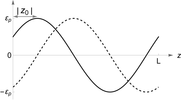
We consider a nonmagnetic medium at $0\leq z\leq L$, whose dielectric coefficient is modulated according to

$$\epsilon\left(z\right)=\epsilon_{h}+\epsilon_{p}e^{i2\beta\left(z+z_{0}\right)}.$$

(1)

where $\beta=\pi/L$ is half the wavenumber of the modulation. Note that when $z_{0}=0$ or $L/2$, the dielectric coefficient satisfy the necessary condition for $\mathcal{PT}$ symmetry, namely, $\epsilon\left(-z\right)=\epsilon^{*}\left(z\right)$. (The particular case of $z_{0}=0$ was considered in Refs. [28, 26, 32, 50], for normal incident waves.) Two homogeneous nonmagnetic waveguides with a dielectric constant $\epsilon_{h}$ are connected at $z\leq 0$ and $z\geq L$, guiding oblique monochromatic waves to- and from the modulated medium (Fig. 1). We focus on TE (or $H$) modes [49], such that the electric field is in the $y$ direction, and propagates in the $xz$ plane. The governing equation for these modes is

$$\left[\partial_{x}^{2}+\partial_{z}^{2}+\frac{\omega^{2}}{c^{2}}\epsilon\left(z\right)\right]E\left(x,z\right)=0,$$

(2)

where $c$ is the speed of light, and we consider time dependency of the form $e^{-i\omega t}$ with an angular frequency $\omega$. The solution in the homogeneous waveguides is given by

$$E\left(x,z\right)=\begin{cases}A_{1}e^{ik_{h}\left(x\cos\theta+z\sin\theta\right)}+B_{1}e^{ik_{h}\left(x\cos\theta-z\sin\theta\right)}&z\leq 0,\\ A_{2}e^{ik_{h}\left[x\cos\theta-\left(z-L\right)\sin\theta\right]}+B_{2}e^{ik_{h}\left[x\cos\theta+\left(z-L\right)\sin\theta\right]}&z\geq L,\end{cases}$$

(3)

where $A_{1}$ and $A_{2}$ ($B_{1}$ and $B_{2}$) are the amplitudes of the incoming (outgoing) waves, $k_{h}=\omega\sqrt{\epsilon_{h}}/c$, and $\theta$ is the angle between the $xy$ plane and the waves in these waveguides.

Inside the modulated medium, we seek solutions in the form

$$E\left(x,z\right)=e^{ik_{h}x\cos\theta}Z\left(z\right),$$

(4)

where the $x$ dependency is enforced by the continuity of $E$ at $z=0$ and $L$. By substituting the ansatz (4) into Eq. (2), we obtain the following equation for $Z\left(z\right)$

$$\left[\partial_{z}^{2}+\frac{\omega^{2}}{c^{2}}\left(\epsilon_{h}+\epsilon_{p}e^{i2\beta\left(z+z_{0}\right)}\right)-k_{h}^{2}\cos^{2}\theta\right]Z\left(z\right)=0,$$

(5)

which can rearranged as

$$\left[\partial_{z}^{2}+k_{h}^{2}\sin^{2}\theta\left(1+\frac{1}{\sin^{2}\theta}\frac{\epsilon_{p}}{\epsilon_{h}}e^{i2\beta\left(z+z_{0}\right)}\right)\right]Z\left(z\right)=0.$$

(6)

Our next step is to rewrite Eq. (6) as a Bessel equation. To this end, we perform a change of variable, namely,

$$\zeta=\sqrt{\frac{k_{h}^{2}\epsilon_{p}}{-\beta^{2}\epsilon_{h}}}e^{i\beta\left(z+z_{0}\right)},$$

(7)

such that

$$\partial_{z}\zeta=i\beta\zeta,\quad\partial_{z}^{2}\zeta=-\beta^{2}\zeta,$$

(8)

which together with the chain rule $\partial_{z}Z=\partial_{\zeta}Z\partial_{z}\zeta$ allows us to replace Eq. (6) with

$$\left[\zeta^{2}\partial_{\zeta}^{2}+\zeta\partial_{\zeta}+\left(\zeta^{2}-\frac{k_{h}^{2}}{\beta^{2}}\sin^{2}\theta\right)\right]Z=0.$$

(9)

Eq. (9) is solved exactly using the Bessel functions $J_{\pm\nu}\left(\zeta\right)\eqqcolon\psi_{\pm}\left(z\right)$, where $\nu=\left(k_{h}/\beta\right)\sin\theta$ is assumed to be a non-integer number. Essentially, Eq. (9) and its solution are generalizations of the results in Refs. [32, 26, 50] to oblique waves. The electric field in the modulated medium is a linear combination of these solutions, such that

$$E\left(x,0\leq z\leq L\right)=C_{1}e^{ik_{h}x\cos\theta}\psi_{+}\left(z\right)+C_{2}e^{ik_{h}x\cos\theta}\psi_{-}\left(z\right).$$

(10)

Our next objective is to related the amplitudes of the waves inside the modulated medium to the amplitudes in the homogeneous waveguides. To this end, we assemble the two quantities that are continuous along $z$, i.e., $E$ and $\partial_{z}E$, into a column vector which we denote by $\mathsf{s}$. In the modulated medium, this so-called state vector can be written as

$$\mathsf{s}\left(0\leq z\leq L\right)=\mathsf{Q}\left(z\right)\mathsf{c},$$

(11)

where

$\displaystyle\text{$\mathsf{Q}$}\left(z\right)=\left(\begin{array}[]{cc}\psi_{+}\left(z\right)&\psi_{-}\left(z\right)\\ \partial_{z}\psi_{+}\left(z\right)&\partial_{z}\psi_{-}\left(z\right)\end{array}\right),\mathsf{c}=\left(\begin{array}[]{c}C_{1}\\ C_{2}\end{array}\right).$

Similarly, the state vector in the right- and left ends of the left- and right homogeneous waveguides is

$$\mathsf{s}\left(0^{-}\right)=\mathsf{Q}_{h}\mathsf{l},\quad\mathsf{s}\left(L^{+}\right)=\mathsf{Q}_{h}\mathsf{r},$$

(12)

respectively, where

$\displaystyle\mathsf{Q}_{h}$

$\displaystyle=\left(\begin{array}[]{cc}1&1\\ ik_{h}\sin\theta&-ik_{h}\sin\theta\end{array}\right),\mathsf{l}=\left(\begin{array}[]{c}A_{1}\\ B_{1}\end{array}\right),\mathsf{r}=\left(\begin{array}[]{c}A_{2}\\ B_{2}\end{array}\right).$

It now follows that from the continuity of the state vector at $z=0$ and $L$, we obtain

$$\mathsf{Q}_{h}\mathsf{l}=\text{\text{$\mathsf{Q}$}$\left(0\right)$}\mathsf{c},\ \mathsf{Q}_{h}\mathsf{r}=\text{\text{$\mathsf{Q}$}$\left(L\right)$}\mathsf{c}.$$

(13)

Accordingly, the transfer matrix $\mathsf{M}$ that relates between the wave amplitudes of the two homogeneous waveguides is

$$\mathsf{M}=\mathsf{Q}_{h}^{-1}\text{$\mathsf{Q}$}\left(L\right)\text{$\mathsf{Q}$}^{-1}\left(0\right)\mathsf{Q}_{h},\ \text{such\ that}\ \mathsf{r}=\mathsf{M}\mathsf{l};$$

(14)

this completes the solution for the electric waves, given any amplitude of incoming waves. Using the Bessel’s continuation rule we have that $\text{$\mathsf{Q}$}\left(L\right)=\text{$\mathsf{Q}$}\left(0\right)\left(\begin{array}[]{cc}e^{ik_{h}\sin\theta L}&0\\ 0&e^{-ik_{h}\sin\theta L}\end{array}\right)$, which together with Eq. (14) yields $\det\mathsf{M}=1$.

We can now relate the incoming and outgoing waves in terms of the components of $\mathsf{M}$. One way to do that is

$$\left(\begin{array}[]{c}B_{1}\\ B_{2}\end{array}\right)=\mathsf{S}\left(\begin{array}[]{c}A_{1}\\ A_{2}\end{array}\right),\ \mathsf{S}=\left(\begin{array}[]{cc}M_{12}/M_{22}&M_{22}^{-1}\\ M_{22}^{-1}&-M_{21}/M_{22}\end{array}\right).$$

(15)

If we prescribe an incoming wave with unitary amplitude from the left (right), such that $A_{1}=1$ and $A_{2}=0$ ($A_{1}=0$ and $A_{2}=1$), it follows that the amplitude of the transmitted wave is $S_{21}$ ($S_{12}$), and the amplitude of the reflected wave is $S_{11}$ ($S_{22}$). Accordingly, the components of $\mathsf{S}$ are identified with the reflection and transmission coefficients, such that

$$\mathsf{S}=\begin{pmatrix}r_{L}&t\\ t&r_{R}\end{pmatrix}.$$

(16)

The eigenvalues of $\mathsf{S}$ are

$$\lambda^{\left(\mathsf{S}\right)}_{1,2}=\frac{r_{L}+r_{R}}{2}\pm\sqrt{\frac{\left(r_{L}-r_{R}\right)^{2}}{4}+t^{2}};$$

(17)

they become degenerate, together with their eigenvectors, when $\left(r_{L}-r_{R}\right)/t=\pm 2i$. These exceptional points of $\mathsf{S}$ for a $\mathcal{PT}$-symmetric scatterer are linked to the degeneracies in its eigenmodes, if it was bounded [2].

There is an alternative scattering matrix, denoted here $\tilde{\mathsf{S}}$, that is obtained if we interchange the two entries of the column vector in the left-hand-side of Eq. (15). By doing so, we obtain

$$\left(\begin{array}[]{c}B_{2}\\ B_{1}\end{array}\right)=\tilde{\mathsf{S}}\left(\begin{array}[]{c}A_{1}\\ A_{2}\end{array}\right),\ \tilde{\mathsf{S}}=\begin{pmatrix}t&r_{R}\\ r_{L}&t\end{pmatrix}.$$

(18)

Both Eq. ,(15) and Eq. (18) deliver the same relations between the incoming and outgoing waves, however the corresponding scattering matrices have different eigenvalues. Specifically, the eigenvalues of $\tilde{\mathsf{S}}$ are

$$\lambda^{\left(\tilde{\mathsf{S}}\right)}_{1,2}=t\pm\sqrt{r_{L}r_{R}};$$

(19)

they become degenerate when either $r_{L}$ or $r_{R}$ vanish. When the scatterer is $\mathcal{PT}$-symmetric, the exceptional points of $\tilde{\mathsf{S}}$ reflect anisotropic transmission resonances (ATRs), at which the reflection may vanish only from one side while the transmittance is unity, since the scattering coefficients for $\mathcal{PT}$-symmetric system satisfy

$$\left|T-1\right|=\sqrt{R_{L}R_{R}},$$

(20)

where $T\coloneqq\left|t\right|^{2}$ is the transmittance, and $R_{L,R}\coloneqq\left|r_{L,R}\right|^{2}$ are the two reflectances.

The zeroes of $\mathsf{S}$, which correspond to a zero eigenvalue, reflect a perfectly absorbing medium, while the poles of $\mathsf{S}$, which correspond to an infinite eigenvalue, reflect a lasing oscillator which emits outgoing coherent waves. It is follows that if $\mathsf{S}$ has a zero, then from Eq. (17) we have $t^{2}=r_{L}r_{R}$, thus $\tilde{\mathsf{S}}$ has a zero too. In our case, it also follows that if $\mathsf{S}$ has a pole then $\tilde{\mathsf{S}}$ has a pole too. To show this, we note that

$\displaystyle\sigma_{1}\mathsf{S}^{*}\left(-z_{0}\right)\sigma_{1}$

$\displaystyle=\mathsf{S}^{-1}\left(z_{0}\right),\tilde{\mathsf{S}}^{*}\left(-z_{0}\right)=\tilde{\mathsf{S}}^{-1}\left(z_{0}\right),$

(21)

where $\sigma_{1}$ is the first Pauli matrix, since $\epsilon\left(z\right)$ satisfies Eq. (1). As a result, the product of the modulus of the eigenvalues of $\mathsf{S}\left(-z_{0}\right)$ and $\mathsf{S}\left(z_{0}\right)$ must be $1$, and the same holds for $\tilde{\mathsf{S}}$. Therefore if $\mathsf{S}\left(z_{0}\right)$ has a pole then $\mathsf{S}\left(-z_{0}\right)$ has a zero, and hence $\tilde{\mathsf{S}}\left(-z_{0}\right)$ has a zero too, which finally implies that $\tilde{\mathsf{S}}\left(z_{0}\right)$ has a pole. In the next section, we analyze the dependency of the zeroes, poles and EPs of $\mathsf{S}$ and $\tilde{\mathsf{S}}$, and the scattering properties, on the system parameters, and specifically the incident angle.

In our case study, we set $\text{$\epsilon_{h}$}=4$, and study the scattering properties as functions of the remaining parameters of the system. We begin with Fig. 2a, where we evaluate the logarithm of the transmittance $T$ (solid black), and the logarithm of the two reflectances $R_{L/R}$ (dash-dotted green and dashed blue) as functions of the incident angle $\theta$, setting the rest of the parameters to

$$\xi\coloneqq\frac{\epsilon_{p}}{\epsilon_{h}}=10^{-1/2},\frac{\beta}{k_{h}}=\frac{1}{\sqrt{2}},z_{0}=0;$$

(22)

and recall that since $z_{0}=0$, the scatter is $\mathcal{PT}$-symmetric. We observe that $T$ varies from $0$ at $\theta=0$, to an anomalous peak of $T=2.63$ at $\theta=0.25$. Notably, the reflectance from the right and left are different, where $R_{L}$ vanishes at $\theta=0.12$ and $\theta=0.77$, there the transmittance is unity. These angles correspond to unidirectional reflection that occurs at the EPs of $\tilde{\mathsf{S}}$, as was first reported by Lin et al. 2011 for the case of normal incident wave. To show this, we plot in Fig. 2b the logarithm of the magnitude of $\lambda^{\left(\tilde{\mathsf{S}}\right)}_{1,2}$ as function of the incident angle $\theta$. Indeed, we observe that there is a transition from unimodular eigenvalues to non-unimodular eigenvalues at $\theta=0.12$ and $\theta=0.77$.

Ge et al. 2012 made the observation that while unidirectional reflectivity occurs at the EPs of $\tilde{\mathsf{S}}$, the EPs of $\mathsf{S}$ are those that capture the breaking of the $\mathcal{PT}$ symmetry of the system. These EPs are analyzed in Fig. 2c, where we evaluate the logarithm of the magnitude of $\lambda^{\left(\mathsf{S}\right)}_{1,2}$ as function of the incident angle. We observe that for $0<\theta<0.44$, the eigenvalues are non-unimodular, and are associated with broken $\mathcal{PT}$ symmetry. $\mathcal{PT}$ symmetry is restored at $\theta=0.44$ , as the eigenvalues become unimodular again. Specifically, both the eigenvalues and eigenvectors coalesce at $\theta=0.44$, which identifies this angle as the EP of $\mathsf{S}$. Note that while the modulus of both the eigenvalues is unity beyond this point, the eigenvalues themselves are different.

To examine the dependency of the $\mathcal{PT}$ symmetry breaking on the amplitude of the modulation, we evaluate in Fig. 3 the EPs of $\mathsf{S}$ for $\xi=10^{-2}$ (red), $10^{-1}$ (blue) and $10^{-1/2}$ (green), as functions of $\omega L/c$ [panel (a)], and $\beta/k_{h}$ [panel (b)]. We highlight the regions that are associated with broken $\mathcal{PT}$ symmetry when $\xi=10^{-2}$, $10^{-1}$ and $10^{-1/2}$ by the light gray, gray and dark gray, respectively. We observe that as we increase the amplitude of the perturbation, the region of the broken phase is extended to lower frequencies, or equivalently greater $\beta/k_{h}$, and higher incident angles.

Having evaluated the phase diagram of $\mathsf{S}$, we proceed to the phase diagram of $\tilde{\mathsf{S}}$, shown in Fig. 4. Specifically, panels $\left(\text{a}\right)$, $\left(\text{b}\right)$ and $\left(\text{c}\right)$ correspond to $\xi=10^{-2}$ (red), $10^{-1}$ (blue) and $10^{-1/2}$ (green), respectively. Here, we distinguish between EPs associated with $r_{L}$ and $r_{R}$ by light and dark shades, respectively. In contrast with the phase diagram of $\mathsf{S}$, which shows that there is at most one EP for a given $\xi$ and $\beta/k_{h}$, here there could be multiple EPs. For example, there are six EPs when $\xi=10^{-1}$ and $\beta/k_{h}=0.32$ (black vertical line in Fig. 4b).

In all the panels, there is a broken region that extends to $\beta/k_{h}=1$. Interestingly, this region is bounded from above by the function $\beta=k_{h}\sin\theta$, which corresponds to the first Fabry-Pérot resonance [24]. In the Appendix, we have used a multiple scale expansion to derive an approximated solution, under the assumption $\beta\approx k_{h}\sin\theta$ and that the perturbation is small, resembling the case studied by Lin et al. 2011; using this approximation, we show that indeed the scatterer exhibits unidirectional reflection under these assumptions. In fact, all Fabry-Pérot resonances, i.e., $m\beta=k_{h}\sin\theta$ for any $m\in\mathbb{N}$, provide an approximation for the EPs of $\tilde{\mathsf{S}}$. These approximations for $m=0..10$ are depicted in magenta lines.

The quality of the Fabry-Pérot resonances approximation depends on how small the perturbation and detuning are. To show this, we use our analytical expressions for $r_{L}$ and $r_{R}$ [Eqs. (14)-(16)] to find that they are proportional to

$\displaystyle r_{L}\propto I_{-\left(\nu+1\right)}\left(\nu\sqrt{\tilde{\xi}}\right)$

$\displaystyle,\quad r_{R}\propto I_{-\left(\nu-1\right)}\left(\nu\sqrt{\tilde{\xi}}\right),$

(23)

where $I$ is the modified Bessel function of the first kind, and we recall that $\nu=\left(k_{h}/\beta\right)\sin\theta$. The modified Bessel function vanishes in the limit $\tilde{\xi}\rightarrow 0^{+}$ when its order is a nonzero integer, i.e., $\nu\rightarrow m\neq 1$, in line with our assumptions. When $\nu$ is close to an even (odd) number from above (below), then $I_{-\left(\nu-1\right)}$ and $I_{-\left(\nu+1\right)}$ vanish for some small positive number. This corresponds to vanishing $r_{L}$ and $r_{R}$ at some small perturbation amplitude $\tilde{\xi}$, near a Fabry-Pérot resonance of even (odd) integer. Exceptions for this rule are for (i) $I_{0}$, which is nonzero at $\tilde{\xi}=0$, hence $r_{R}$ does not vanish in the limit $\nu\rightarrow 1$ that is associated with the first Fabry-Pérot resonance $\left(m=1\right)$; (ii) when $\nu\rightarrow 0^{+}$, $r_{R}$ is proportional to $I_{1^{-}}$, which does not vanish at some small positive number, hence $r_{R}$ does not vanish for $m=0$.

Indeed, we observe that for smallest modulation (Fig. 4a), almost all of the magenta lines coincide with the EPs that we find using the exact solution, including the zeroth order, i.e., when $\theta=0$. By contrast, for the largest modulation (Fig. 4c), the zeroth order does not provide a good approximation at all, and the first order begins to coincide with the exact solution only from $\beta/k_{h}\approx 0.5$.

By analyzing how the zeros of the modified Bessel functions depend on the order, we deduce that the EPs associated with vanishing $r_{L}$ will always be closer to the Fabry-Pérot resonances than those of vanishing $r_{R}$. Since higher Fabry-Pérot resonances become closer in the $\left(\beta/k_{h},\theta\right)$ space, and the approximated solution improves at smaller modulation amplitude and higher order, the EPs of $r_{L}$ and $r_{R}$ become closer at smaller modulations and higher Fabry-Pérot resonances; from a certain frequency, they practically coincide. Thus, this trend provides guidelines for achieving bidirectional zero-reflection.

To demonstrate this, we evaluate in the remaining panels the logarithm of $T$ (solid black), and the two reflectances $R_{L/R}$ (dash-dotted green and dashed blue) as functions of the incident angle $\theta$, for the three different modulations, when setting $\beta/k_{h}=1/4$. Specifically, panels $\left(\text{d}\right)$, $\left(\text{e}\right)$ and $\left(\text{f}\right)$ correspond to $\xi=10^{-2}$, $10^{-1}$ and $10^{-1/2}$, respectively. Panel (d) shows that $R_{L}$ vanishes at $\theta=0.01,0.25,0.52$ and $0.85$, as denoted by the cross marks, while $R_{R}$ vanishes very closely to the latter two angles, i.e., near $\theta=0.52$ and $0.85$, as designated by the circle marks. This observation is in agreement with panel (a), where the wavenumber ratio $\beta/k_{h}=1/4$ is denoted by the dashed line. This line intersects the exceptional line that is near the zeroth Fabry-Pérot resonance at $\theta=0.01$, and then intersects the exceptional lines that practically coincide with the Fabry-Pérot resonances that are defined by $m=$1, 2 and 3. Indeed, near Fabry-Pérot resonances for which $m$ equals zero and one, there is no EP that is associated with $R_{R}$, while near the higher order Fabry-Pérot resonances, i.e., two and three, there are pairs of EPs of $R_{L}$ and $R_{R}$ that are very close to each other about $\theta=0.52$ and $0.85$. Panel (e) shows that $R_{L}$ vanishes at $\theta=0.17,0.18,0.53$ and $0.85$; here, since the modulation amplitude is greater than in panel (d), the angles at which $R_{R}$ vanishes, namely, $\theta=0.73$ and $0.75$, are not as close to the nearest angles at which $R_{L}$ vanishes. Again, these EP observations agree with the way in which the dashed line that denotes $\beta/k_{h}=1/4$ intersects the exceptional lines and the Fabry-Pérot resonances. Finally, we see that in Panel (f), which corresponds to the larger modulation amplitude, there are no angles at which $R_{R}$ vanishes, nor vanishing values $R_{L}$ near the two lowest-order Fabry-Pérot resonances (zero and one), but only from order two.

The analysis so far was for a zero modulation phase, yielding a $\mathcal{PT}$-symmetric scatterer. We recall that when $z_{0}=L/2$, the scatterer is also $\mathcal{PT}$-symmetric: this case is analyzed next. We begin with Fig. 5, which is the same as Fig. 2, only for $z_{0}=L/2$. A comparison between panels 2a and 5a shows that while only $R_{L}$ vanishes (twice) when $z_{0}=0$, when $z_{0}=L/2$ both $R_{L}$ and $R_{R}$ vanish once, at different angles. A comparison of the remaining two panels in Figs. 2 and 5 shows that while the broken region of $\tilde{\mathsf{S}}$ is similar for $z_{0}=0$ and $L/2$, the broken region of $\mathsf{S}$ is completely different, since when $z_{0}=L/2$, $\mathsf{S}$ is always at the $\mathcal{PT}$-symmetric phase for the same given scattering parameters. A more complete picture of the difference in the phase diagrams of the two $\mathcal{PT}$-symmetric systems is given next, by providing the diagrams that are associated with $z_{0}=L/2$. We start with Fig. 6, which shows the EPs of $\mathsf{S}$ as functions of $\theta$ versus $\omega L/c$ [panels (a-c)], and $\beta/k_{h}$ [panels (d-f)] for $\xi=10^{-2}$ [red, panels (a) and (d)], $10^{-1}$ [blue, panels (b) and (e)] and $10^{-1/2}$ [green, panels (c) and (f)], where the broken regions are highlighted with gray. A comparison with the diagram of $z_{0}=0$ (Fig. 3) shows that $z_{0}=L/2$ has a much richer diagram, exhibiting multiple re-entries to the broken region when either one of the three parameters ($\theta$, $\omega$ and $\beta$) is varied. This is in sharp contrast with a single entry when $z_{0}=0$. In addition, when $z_{0}=0$, the broken region of the greater modulations encloses the broken region of the smaller modulations, while when $z_{0}=L/2$, there are regions that belong to the broken phase of smaller modulations, while belonging to the exact phase of greater modulations.

In Fig. 7 we also evaluate the phase diagram of $\tilde{\mathsf{S}}$ in the ($\theta,\beta/k_{h}$) space; panels (a-c) correspond to $\xi=10^{-2}$, $10^{-1}$ and $10^{-1/2}$, where the EPs are highlighted in red, blue and green, respectively, and the broken regions are in gray. We distinguish between the EPs that are associated with zero $r_{L}$ and $r_{R}$ by light and dark shades, respectively. There is some similarity with the diagram of $z_{0}=0$, however here the structure is more complicated and the broken regions are larger.

Here again, all Fabry-Pérot resonances provide an approximation for the EPs of $\tilde{\mathsf{S}}$, and these approximations for $m=0..10$ are depicted in magenta lines. Now we find that the expressions for $r_{L}$ and $r_{R}$ are proportional to the Bessel functions

$\displaystyle r_{L}\propto J_{-\left(\nu+1\right)}\left(\nu\sqrt{\tilde{\xi}}\right)$

$\displaystyle,\quad r_{R}\propto J_{-\left(\nu-1\right)}\left(\nu\sqrt{\tilde{\xi}}\right)J_{\left(\nu-1\right)}\left(\nu\sqrt{\tilde{\xi}}\right).$

(24)

In contrast with the behavior of the modified Bessel functions in Eq. (23), the Bessel functions in Eq. (24) vanish at some positive argument when $\nu$ approaches to a positive integer number from below. This corresponds to vanishing $r_{L}$ and $r_{R}$ at some small perturbation amplitude $\tilde{\xi}$, near a Fabry-Pérot resonance. Here there is only one exception to this rule, namely, that $r_{R}$ does not vanish in the limit $\nu\rightarrow 1$, which is associated with the Fabry-Pérot resonance, i.e., $m=1$.

We proceed to analyze scatterers that do not satisfy $\mathcal{PT}$ symmetry, by considering three exemplary values of $z_{0}$ that are different from 0 and $L/2$. This is carried out in Fig. 8, where we evaluate the logarithm of $T$ and $R_{L/R}$ as functions of $\theta$, setting $\xi=10^{-1/2}$ and $\beta/k_{h}=2^{-1/2}$. Specifically, panels $\left(\text{a}\right)$, $\left(\text{b}\right)$ and $\left(\text{c}\right)$ correspond to $z_{0}=-1/10,3/10$ and $-2/5$, respectively. While $R_{L}$ vanish near $\theta=\pi/4$ in all the panels (corresponding to $\nu=1$), overall there is a strong variation in the scattering properties from one $z_{0}$ to another. For example, when $z_{0}/L=-1/10$, $T$ peaks at $\theta=0.57$ to $1.34$, and then decays to $1.01$ at $\theta=\pi/2$. By contrast, when $z_{0}/L=3/10$, $T$ peaks at $\theta=0.82$ to $1.11$, and then decays to $1.04$ at $\theta=\pi/2$. Furthermore, when $z_{0}/L=-1/10$, $R_{L}$ is unity at $\theta=0$, decays to $0.09$ at $\theta=0.13$ which is a local minimum, then peaks to $0.14$ at $\theta=0.29$, and then decays to zero at $\theta=0.78$, and increases again to $0.01$ at $\theta=\pi/2$. By contrast, when $z_{0}/L=3/10$, the peaks of $R_{L}$ is at $\theta=0$, from which it decays to zero at $\theta=0.79$ and increases again to $0.01$ at $\theta=\pi/2$. The most interesting result is observed for $z_{0}/L=-2/5$ about $\theta=0.09$, where $T,R_{R}$ and $R_{L}$ all peak to giant values at the order of $10^{4}.$

The extreme scattering values in the latter case hint at the existence of a pole of the scattering matrix near $z_{0}/L=-2/5$ and $\theta=0.09$. This observation motivates us to evaluate the eigenvalues of the scattering matrix eigenvalues in the $\left(\theta,z_{0}/L\right)$ space. By doing so, we can identify the poles and zeroes of the scattering matrix, which we plot in Fig. 9 using black circles and red crosses, respectively, for $\xi=10^{-2}$ $\left[\text{panel }\left(\text{a}\right)\right]$, $10^{-1}$ $\left[\text{panel }\left(\text{b}\right)\right]$ and $10^{-1/2}$ $\left[\text{panel }\left(\text{c}\right)\right]$, when $\beta/k_{h}=1/30$. We observe that the poles and zeroes are distributed symmetrically with respect to the $\mathcal{PT}$-symmetric perturbation $z_{0}=0$, namely, if at a certain $\left(z_{0},\theta\right)$ pair there is a pole (zero) then at $\left(-z_{0},\theta\right)$ there is a zero (pole). This is in accordance with our analysis in Sec. 3, where we showed that product of the modulus of the eigenvalues of $\mathsf{S}\left(-z_{0}\right)$ and $\mathsf{S}\left(z_{0}\right)$ is $1$. Such distribution is similar to the symmetric distribution of poles and zeroes in the complex frequency plane that was studied by Ge et al. 2012. There, this distribution resulted from the $\mathcal{PT}$ symmetry of the medium, while in our case, it is a consequence of Eq. (21).

A comparison of the different panels in Fig. 9 shows that by increasing the amplitude of the modulation, the number of poles and zeroes increases too. The collection of all these points constitutes an arc-like structure, whose tip is associated with the angle at which $\mathcal{PT}$ transition occurs for the $\mathcal{PT}$-symmetric system defined by $z_{0}=0$. To show this, we evaluate the logarithm of the eigenvalues of $\mathsf{S}$ when $z_{0}=0$ as function of $\theta$. Specifically, panels (d)-(f) correspond to $\xi=10^{-2},10^{-1}$ and $10^{-1/2}$, respectively; we highlight the broken region at which the eigenvalues are non-unimodular by gray. Indeed, we observe how the tip of the arc-like structure and the transition angle from gray to white coincide. While we are unable to derive a mathematical explanation for this observation, we note that similar observations were made in Refs. [7, 17], which were later explained in Ref. [2]. Specifically, figure 8 in Ref. [17] shows that at the phase transition of the $\mathsf{S}$ matrix there is an anticrossing of the poles in the complex frequency plane, see also figure 3 in Ref. [7]. There, the symmetric distribution of the poles and zeros about the imaginary axis is a result of the $\mathcal{PT}$ symmetry of the system; here, the $\left(\theta,z_{0}\right)$ space plays a similar role, where the symmetric distribution of the poles and zeros is about $z_{0}=0$, owing to Eq. (21).

Fig. 9f also displays a divergence of the eigenvalues, as one of them tends to explode and the other tends to vanish. This is in accordance with the proximity of a zero and a pole near $z_{0}=0$ in panel (c), where we recall that their overlap corresponds to CPA-laser states. We thus refer to these states, where a zero and pole are very close but not coincide, as a quasi CPA-laser state. In such states, as we highlight next, one of the eigenvalues tends to vanish, but remains greater from zero, while the other grows significantly, but remains finite. This behavior of the eigenvalues implies that the scatterer can simultaneously absorb almost completely incoming coherent waves and significantly enhance certain incoherent excitations.

Quasi CPA-laser states occur also, e.g., for $\xi=10^{-2}$ at $\theta\approx 0.12$, when $z_{0}/L\approx\pm 0.1$. We examine in Fig. 10 how the logarithm of the eigenvalues modulus of $\mathsf{S}$ vary near these states as function of two different variables: (i) $z_{0}/L$ when theta is fixed to $\approx 0.12$ [panel (a)]; and (ii) $\theta$ when $z_{0}/L$ is fixed to $z_{0}\approx 0.1$ [panel (b)], while the rest of the parameters are set to $\beta/k_{h}=1/30$ and $\xi=10^{-2}$. We observe in panel (a) the symmetric distribution of each one of the eigenvalues with respect to $z_{0}=0$. In addition, we observe how near $z_{0}/L\approx-0.1$ one of them grows and the other diminishes, where near $z_{0}/L\approx 0.1$ their tendency is interchanged. The rapid growth and decay of the eigenvalues near the critical angle $\theta\approx 0.12$ is demonstrated in panel (b).

We derived an exact solution to the problem of monochromatic oblique TE waves that are scattered by a waveguide with sinusoid gain-loss modulation. We have analyzed a family of modulations that are parametrized by their phase, amplitude and wavelength. We have investigated how these parameters, together with the frequency and incident angle of the waves, affect the emergence of lasing, perfect absorption, and anisotropic transmission resonances. For two particular modulations that satisfy $\mathcal{PT}$ symmetry, we have evaluated the diagram of the exact- and broken $\mathcal{PT}$ phases in the parameter space, and the phase diagram that defines the anisotropic transmission resonances. The two modulations have different diagrams, one of which is much richer, exhibiting multiple re-entries to the broken region. With regard to the diagrams of the anisotropic transmission resonances, we have showed that there is a regime in the parameter space where these resonances reside very close to Fabry-Pérot resonances. A further investigation of this property has provided guidelines on how to design bidirectional zero-reflection states. Finally, we have analyzed the poles and zeros of the scattering matrix, which correspond, respectively, to lasing and perfect absorption states. We showed that the the modulation phase and incident angle constitute a design space for these singularities when the scatterer is subjected to monochromatic waves. Specifically, we have identified quasi CPA-laser states, when a zero and pole are very close but not coincide. These states correspond to scatterers that can simultaneously absorb almost completely incoming coherent waves and significantly enhance certain incoherent excitations.

We thank anonymous reviewers for constructive feedback that helped us improve this paper. This research has received funding from the European Research Council (ERC) under the European Union’s Horizon 2020 Research and Innovation Programme, grant agreement no. 101045494 (EXCEPTIONAL), and the Israel Science Foundation, Israel Academy of Sciences and Humanities (Grant no. 2061/20).

References

- Achilleos et al. [2017] V. Achilleos, G. Theocharis, O. Richoux, and V. Pagneux. Non-hermitian acoustic metamaterials: Role of exceptional points in sound absorption. Phys. Rev. B, 95:144303, Apr 2017. doi: 10.1103/PhysRevB.95.144303. URL https://link.aps.org/doi/10.1103/PhysRevB.95.144303.
- Ambichl et al. [2013] Philipp Ambichl, Konstantinos G. Makris, Li Ge, Yidong Chong, A. Douglas Stone, and Stefan Rotter. Breaking of symmetry in bounded and unbounded scattering systems. Phys. Rev. X, 3:041030, Dec 2013. doi: 10.1103/PhysRevX.3.041030. URL https://link.aps.org/doi/10.1103/PhysRevX.3.041030.
- Ashida et al. [2020] Yuto Ashida, Zongping Gong, and Masahito Ueda. Non-hermitian physics. Advances in Physics, 69(3):249–435, 07 2020. doi: 10.1080/00018732.2021.1876991. URL https://doi.org/10.1080/00018732.2021.1876991.
- Bender and Boettcher [1998] Carl M Bender and Stefan Boettcher. Real Spectra in Non-Hermitian Hamiltonians Having PT Symmetry. Phys. Rev. Lett., 80(24):5243–5246, 1998. doi: 10.1103/PhysRevLett.80.5243. URL https://link.aps.org/doi/10.1103/PhysRevLett.80.5243.
- Berry [2004] M. V. Berry. Physics of nonhermitian degeneracies. Czechoslovak Journal of Physics, 54(10):1039–1047, 2004. doi: 10.1023/B:CJOP.0000044002.05657.04. URL https://doi.org/10.1023/B:CJOP.0000044002.05657.04.
- Chong et al. [2010] Y. D. Chong, Li Ge, Hui Cao, and A. D. Stone. Coherent perfect absorbers: Time-reversed lasers. Phys. Rev. Lett., 105:053901, Jul 2010. doi: 10.1103/PhysRevLett.105.053901. URL https://link.aps.org/doi/10.1103/PhysRevLett.105.053901.
- Chong et al. [2011] YD Chong, Li Ge, and A Douglas Stone. P t-symmetry breaking and laser-absorber modes in optical scattering systems. Physical Review Letters, 106(9):093902, 2011.
- Christensen et al. [2016] J Christensen, M Willatzen, V R Velasco, and M.-H. Lu. Parity-Time Synthetic Phononic Media. Phys. Rev. Lett., 116(20):207601, 2016. doi: 10.1103/PhysRevLett.116.207601. URL https://link.aps.org/doi/10.1103/PhysRevLett.116.207601.
- Christodoulides et al. [2018] Demetrios Christodoulides, Jianke Yang, et al. Parity-time symmetry and its applications, volume 280. Springer, 2018.
- Djorwe et al. [2019] P. Djorwe, Y. Pennec, and B. Djafari-Rouhani. Exceptional point enhances sensitivity of optomechanical mass sensors. Phys. Rev. Applied, 12:024002, Aug 2019. doi: 10.1103/PhysRevApplied.12.024002. URL https://link.aps.org/doi/10.1103/PhysRevApplied.12.024002.
- Droulias et al. [2019] Sotiris Droulias, Ioannis Katsantonis, Maria Kafesaki, Costas M. Soukoulis, and Eleftherios N. Economou. Accessible phases via wave impedance engineering with -symmetric metamaterials. Phys. Rev. B, 100:205133, Nov 2019. doi: 10.1103/PhysRevB.100.205133. URL https://link.aps.org/doi/10.1103/PhysRevB.100.205133.
- El-Ganainy et al. [2018] Ramy El-Ganainy, Konstantinos G Makris, Mercedeh Khajavikhan, Ziad H Musslimani, Stefan Rotter, and Demetrios N Christodoulides. Non-Hermitian physics and PT symmetry. Nature Physics, 14:11 EP –, 2018. URL https://doi.org/10.1038/nphys4323.
- El-Ganainy et al. [2019] Ramy El-Ganainy, Mercedeh Khajavikhan, Demetrios N. Christodoulides, and Sahin K. Ozdemir. The dawn of non-hermitian optics. Communications Physics, 2(1):37, 2019. doi: 10.1038/s42005-019-0130-z. URL https://doi.org/10.1038/s42005-019-0130-z.
- Elbaz et al. [2022] Guy Elbaz, Adi Pick, Nimrod Moiseyev, and Gal Shmuel. Encircling exceptional points of bloch waves: mode conversion and anomalous scattering. Journal of Physics D: Applied Physics, 2022. URL http://iopscience.iop.org/article/10.1088/1361-6463/ac5859.
- Feng et al. [2017] Liang Feng, Ramy El-Ganainy, and Li Ge. Non-hermitian photonics based on parity–time symmetry. Nature Photonics, 11(12):752–762, 2017. doi: 10.1038/s41566-017-0031-1. URL https://doi.org/10.1038/s41566-017-0031-1.
- Fleury et al. [2015] Romain Fleury, Dimitrios Sounas, and Andrea Alù. An invisible acoustic sensor based on parity-time symmetry. Nature Communications, 6:5905, 2015. ISSN 2041-1723. doi: 10.1038/ncomms6905. URL http://www.nature.com/doifinder/10.1038/ncomms6905.
- Ge et al. [2012] Li Ge, YD Chong, and A Douglas Stone. Conservation relations and anisotropic transmission resonances in one-dimensional pt-symmetric photonic heterostructures. Physical Review A, 85(2):023802, 2012.
- Geng et al. [2021] Linlin Geng, Weixuan Zhang, Xiangdong Zhang, and Xiaoming Zhou. Topological mode switching in modulated structures with dynamic encircling of an exceptional point. Proceedings of the Royal Society A: Mathematical, Physical and Engineering Sciences, 477(2245):20200766, 2021. doi: 10.1098/rspa.2020.0766. URL https://royalsocietypublishing.org/doi/abs/10.1098/rspa.2020.0766.
- Goldzak et al. [2018] Tamar Goldzak, Alexei A Mailybaev, and Nimrod Moiseyev. Light Stops at Exceptional Points. Phys. Rev. Lett., 120(1):13901, 2018. doi: 10.1103/PhysRevLett.120.013901. URL https://link.aps.org/doi/10.1103/PhysRevLett.120.013901.
- Graefe and Jones [2011] Eva-Maria Graefe and H. F. Jones. -symmetric sinusoidal optical lattices at the symmetry-breaking threshold. Phys. Rev. A, 84:013818, Jul 2011. doi: 10.1103/PhysRevA.84.013818. URL https://link.aps.org/doi/10.1103/PhysRevA.84.013818.
- Heiss [2016] Dieter Heiss. Circling exceptional points. Nature Physics, 12(9):823–824, 2016. doi: 10.1038/nphys3864. URL https://doi.org/10.1038/nphys3864.
- Heiss [2012] W D Heiss. The physics of exceptional points. Journal of Physics A: Mathematical and Theoretical, 45(44):444016, oct 2012. doi: 10.1088/1751-8113/45/44/444016. URL https://doi.org/10.1088/1751-8113/45/44/444016.
- Hodaei et al. [2017] Hossein Hodaei, Absar U Hassan, Steffen Wittek, Hipolito Garcia-Gracia, Ramy El-Ganainy, Demetrios N Christodoulides, and Mercedeh Khajavikhan. Enhanced sensitivity at higher-order exceptional points. Nature, 548(7666):187, 2017.
- Hodgson and Weber [2005] N. Hodgson and H. Weber. Optical Resonators: Fundamentals, Advanced Concepts, Applications. Springer Series in Optical Sciences. Springer, 2005. ISBN 9780387400785. URL https://books.google.co.il/books?id=1zNKKnFytjkC.
- Hou et al. [2018] Zhilin Hou, Huiqin Ni, and Badreddine Assouar. Pt-symmetry for elastic negative refraction. Phys. Rev. Applied, 10(4):44071, 2018. doi: 10.1103/PhysRevApplied.10.044071. URL https://link.aps.org/doi/10.1103/PhysRevApplied.10.044071.
- Jones [2012] H F Jones. Analytic results for a pt-symmetric optical structure. Journal of Physics A: Mathematical and Theoretical, 45(13):135306, mar 2012. doi: 10.1088/1751-8113/45/13/135306. URL https://doi.org/10.1088/1751-8113/45/13/135306.
- Katsantonis et al. [2020] Ioannis Katsantonis, Sotiris Droulias, Costas M Soukoulis, Eleftherios N Economou, and Maria Kafesaki. Pt-symmetric chiral metamaterials: asymmetric effects and pt-phase control. Physical Review B, 101(21):214109, 2020.
- Lin et al. [2011] Zin Lin, Hamidreza Ramezani, Toni Eichelkraut, Tsampikos Kottos, Hui Cao, and Demetrios N. Christodoulides. Unidirectional invisibility induced by -symmetric periodic structures. Phys. Rev. Lett., 106:213901, May 2011. doi: 10.1103/PhysRevLett.106.213901. URL https://link.aps.org/doi/10.1103/PhysRevLett.106.213901.
- Liu et al. [2020] Qingjie Liu, Chengzhi Qin, Bing Wang, and Peixiang Lu. Scattering singularities of optical waveguides under complex modulation. Physical Review A, 101(3):033818, 2020.
- Longhi [2018] S. Longhi. Exceptional points and photonic catastrophe. Opt. Lett., 43(12):2929–2932, Jun 2018. doi: 10.1364/OL.43.002929. URL http://ol.osa.org/abstract.cfm?URI=ol-43-12-2929.
- Longhi [2010] Stefano Longhi. -symmetric laser absorber. Phys. Rev. A, 82:031801, Sep 2010. doi: 10.1103/PhysRevA.82.031801. URL https://link.aps.org/doi/10.1103/PhysRevA.82.031801.
- Longhi [2011] Stefano Longhi. Invisibility in $\mathcal PT$-symmetric complex crystals. Journal of Physics A: Mathematical and Theoretical, 44(48):485302, nov 2011. doi: 10.1088/1751-8113/44/48/485302. URL https://doi.org/10.1088/1751-8113/44/48/485302.
- Lustig et al. [2019] Ben Lustig, Guy Elbaz, Alan Muhafra, and Gal Shmuel. Anomalous energy transport in laminates with exceptional points. Journal of the Mechanics and Physics of Solids, page 103719, 2019. ISSN 0022-5096. doi: https://doi.org/10.1016/j.jmps.2019.103719. URL http://www.sciencedirect.com/science/article/pii/S0022509619306921.
- Mailybaev et al. [2005] AA Mailybaev, ON Kirillov, and AP Seyranian. Geometric phase around exceptional points. PHYSICAL REVIEW A, 72(1), JUL 2005. ISSN 1050-2947. doi: {10.1103/PhysRevA.72.014104}.
- Midya et al. [2018] Bikashkali Midya, Han Zhao, and Liang Feng. Non-hermitian photonics promises exceptional topology of light. Nature Communications, 9(1):2674, 2018. doi: 10.1038/s41467-018-05175-8. URL https://doi.org/10.1038/s41467-018-05175-8.
- Miri and Alù [2019] Mohammad-Ali Miri and Andrea Alù. Exceptional points in optics and photonics. Science, 363(6422), 2019. ISSN 0036-8075. doi: 10.1126/science.aar7709. URL https://science.sciencemag.org/content/363/6422/eaar7709.
- Moiseyev [2011] Nimrod Moiseyev. Non-Hermitian Quantum Mechanics. Cambridge University Press, 2011. doi: 10.1017/CBO9780511976186.
- Mostafazadeh [2002] Ali Mostafazadeh. Pseudo-hermiticity versus pt symmetry: The necessary condition for the reality of the spectrum of a non-hermitian hamiltonian. Journal of Mathematical Physics, 43(1):205–214, 2002. doi: 10.1063/1.1418246. URL https://doi.org/10.1063/1.1418246.
- Mostafazadeh [2013] Ali Mostafazadeh. Invisibility and symmetry. Phys. Rev. A, 87:012103, Jan 2013. doi: 10.1103/PhysRevA.87.012103. URL https://link.aps.org/doi/10.1103/PhysRevA.87.012103.
- Özdemir et al. [2019] Ş. K. Özdemir, S. Rotter, F. Nori, and L. Yang. Parity–time symmetry and exceptional points in photonics. Nature Materials, 18(8):783–798, 2019. doi: 10.1038/s41563-019-0304-9. URL https://doi.org/10.1038/s41563-019-0304-9.
- Peng et al. [2016] Bo Peng, Şahin Kaya Özdemir, Matthias Liertzer, Weijian Chen, Johannes Kramer, Huzeyfe Yılmaz, Jan Wiersig, Stefan Rotter, and Lan Yang. Chiral modes and directional lasing at exceptional points. Proceedings of the National Academy of Sciences, 113(25):6845–6850, 2016. ISSN 0027-8424. doi: 10.1073/pnas.1603318113. URL https://www.pnas.org/content/113/25/6845.
- Pick et al. [2017] Adi Pick, Zin Lin, Weiliang Jin, and Alejandro W. Rodriguez. Enhanced nonlinear frequency conversion and purcell enhancement at exceptional points. Phys. Rev. B, 96:224303, Dec 2017. doi: 10.1103/PhysRevB.96.224303. URL https://link.aps.org/doi/10.1103/PhysRevB.96.224303.
- Pilehvar et al. [2022] Elnaz Pilehvar, Ehsan Amooghorban, and Mohammad Kazem Moravvej-Farshi. Oblique propagation of the squeezed states of s(p)-polarized light through non-hermitian multilayered structures. Opt. Express, 30(3):3553–3565, Jan 2022. doi: 10.1364/OE.448229. URL https://opg.optica.org/oe/abstract.cfm?URI=oe-30-3-3553.
- Rüter et al. [2010] Christian E Rüter, Konstantinos G Makris, Ramy El-Ganainy, Demetrios N Christodoulides, Mordechai Segev, and Detlef Kip. Observation of parity–time symmetry in optics. Nature physics, 6(3):192, 2010.
- Shen et al. [2018] Chen Shen, Junfei Li, Xiuyuan Peng, and Steven A. Cummer. Synthetic exceptional points and unidirectional zero reflection in non-hermitian acoustic systems. Phys. Rev. Materials, 2:125203, Dec 2018. doi: 10.1103/PhysRevMaterials.2.125203. URL https://link.aps.org/doi/10.1103/PhysRevMaterials.2.125203.
- Shi et al. [2016] Chengzhi Shi, Marc Dubois, Yun Chen, Lei Cheng, Hamidreza Ramezani, Yuan Wang, and Xiang Zhang. Accessing the exceptional points of parity-time symmetric acoustics. Nature communications, 7:11110, 2016.
- Siegman [1986] A. E. Siegman. Lasers. University Science Books, Mill Valley, Calif., 1986. ISBN 9780935702118 0935702113 0198557132 9780198557135 0685055957 9780685055953.
- Sweeney et al. [2019] William R. Sweeney, Chia Wei Hsu, Stefan Rotter, and A. Douglas Stone. Perfectly absorbing exceptional points and chiral absorbers. Phys. Rev. Lett., 122:093901, Mar 2019. doi: 10.1103/PhysRevLett.122.093901. URL https://link.aps.org/doi/10.1103/PhysRevLett.122.093901.
- Tamir et al. [1964] T. Tamir, H.C. Wang, and A.A. Oliner. Wave propagation in sinusoidally stratified dielectric media. IEEE Transactions on Microwave Theory and Techniques, 12(3):323–335, 1964. doi: 10.1109/TMTT.1964.1125815.
- Uzdin and Moiseyev [2012] R. Uzdin and N. Moiseyev. Scattering from a waveguide by cycling a non-hermitian degeneracy. Physical Review A - Atomic, Molecular, and Optical Physics, 85:031804(R), 2012. ISSN 10502947. URL http://search.ebscohost.com/login.aspx?direct=true&db=edselc&AN=edselc.2-52.0-84859150818&site=eds-live.
- Watts [2012] Robert G Watts. Introduction to perturbation methods. In Essentials of Applied Mathematics for Engineers and Scientists, pages 153–162. Springer, 2012.
- Wiersig [2014] Jan Wiersig. Enhancing the sensitivity of frequency and energy splitting detection by using exceptional points: Application to microcavity sensors for single-particle detection. Phys. Rev. Lett., 112:203901, May 2014. doi: 10.1103/PhysRevLett.112.203901. URL https://link.aps.org/doi/10.1103/PhysRevLett.112.203901.
- Yin and Zhang [2013] Xiaobo Yin and Xiang Zhang. Unidirectional light propagation at exceptional points. Nature Materials, 12(3):175–177, 2013. doi: 10.1038/nmat3576. URL https://doi.org/10.1038/nmat3576.
- Zhao and Feng [2018] Han Zhao and Liang Feng. Parity–time symmetric photonics. National Science Review, 5(2):183–199, 01 2018. ISSN 2095-5138. doi: 10.1093/nsr/nwy011. URL https://doi.org/10.1093/nsr/nwy011.
- Zhong et al. [2019] Q. Zhong, J. Ren, M. Khajavikhan, D. N. Christodoulides, Ş. K. Özdemir, and R. El-Ganainy. Sensing with exceptional surfaces in order to combine sensitivity with robustness. Phys. Rev. Lett., 122:153902, Apr 2019. doi: 10.1103/PhysRevLett.122.153902. URL https://link.aps.org/doi/10.1103/PhysRevLett.122.153902.