A Simplified Algorithm for Identifying Abnormal Changes in Dynamic Networks
Bouchaib Azamir1,a, Driss Bennis1,b and Bertrand Michel2,c
1 Faculty of Sciences, Mohammed V University in Rabat, Morocco.
a bouchaib_azamir@um5.ac.ma
b driss.bennis@um5.ac.ma; drissbennis@hotmail.com
2 Nantes Université, Ecole Centrale Nantes, Laboratoire de mathématiques Jean Leray UMR 6629.
1 Rue de La Noe, 44300 Nantes, France.
c bertrand.michel@ec-nantes.fr
Abstract. Topological data analysis has recently been applied to the study of dynamic networks. In this context, an algorithm was introduced and helps, among other things, to detect early warning signals of abnormal changes in the dynamic network under study. However, the complexity of this algorithm increases significantly once the database studied grows. In this paper, we propose a simplification of the algorithm without affecting its performance. We give various applications and simulations of the new algorithm on some weighted networks. The obtained results show clearly the efficiency of the introduced approach. Moreover, in some cases, the proposed algorithm makes it possible to highlight local information and sometimes early warning signals of local abnormal changes.
2010 Mathematics Subject Classification: 55N35; 55U99; 91B84
Key Words. Persistent homology; closeness centrality in a network; central subnetwork; time series.
1 Introduction
A network is an efficient representation of a given set of entities and the existing relationships between them. Actually a network is a graph which entities are the vertices and the relations between them are presented as edges (see for instance [14] and [17]). Usually, these relations are quantified by (mostly positive) real numbers and in this case we say that the graph (the network) is weighted. In most real-life situations, (weighted) networks evolve over time resulting in a family of (weighted) networks; we then speak of dynamic (weighted) networks (see the beginning of Section 3). In general, there are two kinds of dynamic networks :
- •
There are dynamic networks such that both the set of vertices and the set of edges are changing over time. For instance, chat groups in social networks where the members of these groups are undergoing changes from moment to moment.
- •
In some situations, the set of vertices remains unchanged over time as in the case of financial networks such as the weighted networks representing stock market transactions. So, the only changes occur at the level of the edges and at the level of the weights.
Dynamic networks have been subject of several studies. See for instance the papers and the references within [20, 21, 22, 23, 24] where dynamic networks have been studied following different approaches. In this paper, we are interested in studying the behaviour of dynamic weighted networks using topological data analysis (TDA). In [12], Gidea used TDA to detect the early signs of a financial market crisis. His method is based mainly on the fact that we can associate with any financial network of stocks a metric space whose distance is defined by the correlation coefficients of stock market returns. This allows to compute the so-called persistent homology of this metric space (see the preliminaries in Section 2) and, thanks to the concept of time series, the first signs of a critical transition in the financial network are detected. It is clear that Gidea’s method can be applied on any other dynamic network. However, for large networks, the execution time of the algorithms used in Gidea’s method will be very high. Thus, one can ask whether the fact of working on particular subgraphs rather than the whole network permits to achieve good results in a reasonable amount of time. Indeed, the abundance of real-world data and its velocity usually call for data summarization. Namely, graph summarization is a useful tool to help identify the structure and meaning of data. It has various advantages including reducing data volume and storage, speeding up algorithms and graph queries, eliminating noise, among others. There are different types of graph summaries depending on whether the data is homogeneous or heterogeneous and also whether the network is static or dynamic. In the literature, graph summarization methods use a set of basic techniques, here we are interested in those that are based on simplification or parsimony: these methods rationalize an input graph by removing nodes or edges less “important”, resulting in a sparse graph see [25]. Here, the summary graph consists of a subset of the original nodes and/or edges. A representative work on node simplification-based summarization techniques is OntoVis [30], a visual analysis tool for exploring and understanding large heterogeneous social networks. In [6], the authors propose a four-step unsupervised algorithm for egocentric information abstraction of heterogeneous social networks using edge, instead of node, filtering. In [31], a new problem, to simplify weighted graphs by removing less important edges, has been proposed. Simplified graphs can be used to improve the visualization of a network, to extract its main structure, or as a preprocessing step for other data mining algorithms.
Our approach is part of the simplification of graphs and aims to identify a subnetwork that contains a large part of the information embodied by the original network.
Our aim in this paper is to show that there are some subnetworks that can be good candidates for this study. Those subnetworks are extracted from the whole graph by eliminating some edges at certain threshold which is determined by the use of the closeness centrality concept (see Section 4 for the definition of closeness centrality).
The idea is based on the fact that a node having the highest closeness centrality is able to spread information efficiently through the whole graph (see [28] for more details). Then, based on this fact, we propose that the desired subnetwork would be the one which contains this node called henceforth central node. After that, we need to set the threshold where edges with higher weights will be eliminated. Also, following the closeness centrality notion, the threshold will be chosen from the list of weights of the incident edges to the central node. However, it is not clear how to determine the optimal threshold. This is why we propose to focus our study on the three quartiles, the minimum and the maximum of the above proposed list of weights. The associated subnetworks will be called central subnetworks (see Section 4 for more details about centrality). Our aim is to determine what threshold levels provides good results. We will see throught several examples that when the threshold is greater than the third quartiles, the adopted approach reduces considerably the execution time of Gidea’s method (to almost half in some cases) without compromising quality and results. Moreover, in some cases we get good results even with thresholds greater than the median.
This paper is organized as follows:
Section 2 presents some preliminaries on persistent homology. We start this section with a part (Subsection 2.1) in which we present a short mathematical background that we need to understand the persistent homology associated to weighted graphs (given in Subsection 2.2), and we present also how to implement data to get persistence diagrams associated to weighted graphs (see Subsection 2.3).
In Section 3, we present how to associate persistent homology to dynamic networks (see Subsection 3.1) and show how it was used by Gidea to detect abnormal changes in financial networks (see Subsection 3.2).
Section 4 represents our approach to reduce the computation cost of Gidea’s method (see Figure 5 for the flowchart of the proposed method). It is mainly based on a simplification of the whole studied network by considering what we called central subnetworks determined using the notion of closeness centrality (see Algorithm 1). We also describe how to get the persistence diagrams associated to these central subnetworks (see Algorithm 2).
Section 5 concerns the application phase. Namely, we present some numerical experiments in which we compare our method with existing ones. In each of the first three subsections, we simulate a dynamic network. Each subsection deals with a kind of a weighted network whose vertex point cloud is simulated with a given probability distribution. Then the corresponding central subnetworks are derived. A visual comparison between the time series associated to both the whole network and the central subnetwork shows that are very similar (see Figures in this section). This observation is also confirmed by the calculated R-squared coefficients (see Tables in this section). In parallel, we show that using our method the execution time is reduced considerably (see Tables in this section). We end Section 5 by a comparison a performance comparison between our approach and the edge collapse method (Subsection 5.4). It is known that the edge collapse method provides theoretical guarantees and allows to obtain, in output, the same starting persistence diagram (see for instance [16]). From Table 4, we deduce that our method is more practical for large and dense networks.
We end this article with Section 6 which includes an application of the method on real weighted networks. In Subsection 6.1, we apply on the financial network used by Gidea [12], and in Subsection 7 we consider a cryptocurrency network. As in Section 5, we deduce an improvement of the execution time using the new method.
2 Persistent homology computed on graphs
Persistent homology is an emergent method for detecting geometrical and topological properties of a space endowed with a topological structure. The concept of persistence was first introduced by Edelsbrunner, Letscher and Zomorodian in [8] and then refined by Carlsson and Zomorodian in [3]. Since then, persistent homology has become an essential tool in topological Data Analysis (TDA) and has been applied in various scientific fields such as biology, image processing, sensor networks
etc. Nowadays, there are many references (surveys, books and notes) on TDA; for a recent one we refer to [5].
In this section, we give a short presentation on some basic notions concerning particular simplicial complexes as well as its corresponding persistent homology. We will focus, following our context, on simplicial complexes associated to graphs investigated in [2]. For a general background on persistent homology one can see [3, 5, 7, 11].
2.1 Simplicial complex and simplicial homology groups
We start this subsection with a recall of a simplicial complex and then we give the examples of interest.
Given a finite set , a simplicial complex with the vertex set is a set of finite subsets of such that the elements of belong to and for any , any subset of belongs to . The elements of are called the faces or the simplices of . The dimension of a simplex of is just its cardinality minus 1 and the dimension of the simplicial complex is the largest dimension of its simplices [5].
There are a lot of examples of simplicial complexes arising from various contexts. Here, we use the following ones:
Example 2.1 (Simplicial clique complex, [2])
Let be a graph, where is the set of vertices and the set of edges. For a positive integer , a -clique of is a set of vertices whose the induced subgraph is complete. Denote by the set of all the cliques of . Notice that the set satisfies the two conditions :
- •
contains all singletons with .
- •
is closed under subsets: if and , then .
Then, is a simplicial complex which is called a simplicial clique complex of .
The following (geometric) classical example of simplicial complexes can be found in any introductory books on TDA.
Example 2.2 (Vietoris-Rips complex)
Given a finite set of points in a metric space and a real number . The Vietoris-Rips complex is a simplicial complex whose simplices are sets such that for all .
Now we are ready to recall what are simplicial homology groups of a simplicial complex. To this end, we define some vector spaces and linear maps.
Here, we only deal with vector spaces on the field .
Given a simplicial complex , the vector space generated by the -simplices of is denoted by . It consists of all finite formal sums of -simplices called -chains; i.e., an element belongs to if it can be written as follows: for some scalers and a family of -simplices.
For a positive integer , consider the linear map , called boundary map, defined on -simplices as follows: For every -simplex , is the formal sum of the -dimensional faces (i.e., subsets of of cardinal ). An element of the image of is called a boundary. Thus, the boundary of a chain is obtained by extending linearly; i.e., . The -chains that have boundary are called -cycles. They form a subspace of . The -chains which are the boundary of -chains are called -boundaries and form a subspace of . It is important but not difficult to show that which is equivalent to . Then, if we consider the quotient vector space , that means we have annihilated the -boundaries which are not -cycles. For instance, if we take to be , the simplicial clique complex of a graph , the dimension of the vector space will be exactly the number of “holes” in and the dimension of the vector space is the number of the connected components of (i.e., the connected components of the graph (network) ). For this reason and of course other important ones, the vector space is considered as one of the principal notions in algebraic topology that helps in describing topological features. It is denoted by and usually called the simplicial homology group of . Its elements are called homology classes.
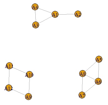
Example 2.3
The simplicial clique complex associated to the graph in Figure 1 has three connected components, and so the dimension of is three. But it has only one hole because is a cycle but not a boundary. Notice that is a boundary of the -chain .
2.2 Persistence diagrams
When a simplicial complex has a history in the sense that it is an union of a chain of simplicial complexes, we can capture more information on ; especially, the behaviour of homology groups of these complexes can be used as a signature of the complex that can be used to distinguish it from other complexes. This is one of many important things that persistent homology is performing.
Consider the following chain of simplicial subcomplexes of a complex , called a filtration of :
This filtration provides more information on K in the following sense: for every couple such that , the injection induces a homomorphism on the simplicial homology groups for each dimension:
The persistent Betti number is the rank of the vector space ; that is, . Persistent Betti numbers count how many homology classes of dimension that survive during the passage from to . We say that a homology class is born entering in , if does not come from a previous subcomplex; that is, . Similarly, if is born in , it dies entering if the image of the map induced by does not contain the image of but the image of the map induced by does. In this case the persistence of is . Finally, all the collected data of births and deaths are presented in a diagram which is the multi-set of points with coordinates correspond respectively to the birth time and the death time of homology classes. This diagram is called an -dimensional persistence diagram, or simply a persistence diagram, of .
As a simple example, the filtration represented in Figure 2 is a filtration of the simplicial clique complex given in Example 2.3.

The -dimensional persistence diagram associated to the filtration given in Figure 2 is given in Figure 3.

Certainly, the persistence diagram of reveals more information on it than those extracted from the (static) complex . Moreover, persistence diagrams can be used to compute the degree of similarity between complexes. To this end, some metric distances are introduced on the space of persistence diagrams. In this paper, we use the so called -Wasserstein distance (for a positive integer ). It is defined by the formula:
where and are two diagrams and varies across all one-to-one and onto functions from to . In this paper we use just the -Wasserstein distance.
Now, to apply the concept above on graph, the notion of weight functions is used as follows: Let be a weighted graphs, where is the set of vertices and the set of edges, such that the weight function is assumed to be upper bounded by a positive real number . Let be the clique complex of . We would like to construct a filtration of (i.e., a chain of complexes that covers ). To do so, let us consider, for every , the sublevel set and the associated subgraph of which will be called the subgraph of at the threshold . Then, we consider the associated clique complex at the level. In particular, . Now, for a sequence of real numbers, we get a filtration of (called Rips filtration):
where . Therefore, the persistent homology, described above, applied on this filtration provides more information on the graph as we will deduce throughout this paper.
2.3 Implementation
Nowadays, there are various softwares for computations of persistent homology and corresponding information. In this article, we often use the R package TDA (for a short tutorial and introduction on the use of the R package TDA, see [10]), except in Subsection 5.4 where we use also the Gudhi library11 1 https://gudhi.inria.fr. We will also use the R software for computations corresponding the time series (see for instance [4]).
In this subsection, we present how to implement the method described in Subsection 2.2 in order to get the persistence diagram of a weighted graph.
It should be noted that the existing software implements data from a metric space. Thus, in order to implement the method described in Subsection 2.2, we need a distance between nodes. The weight function can be used to this end (see Subsection 3.2). So here we assume that the weight function defines a distance between nodes. In other words, the graph with the weight function is a metric space. In this case, the associated clique complexes are nothing but the Vietoris-Rips complexes.
Now, the implementation which provides persistence diagrams of a weighted graph, as it is conceived, deals with matrices of distances associated to a metric space. These matrices are, in our context, matrices of weighted complete graphs. Then, given a weighted complete graph , one can determine its persistence diagram by using the Rips filtration method such that the max-scale of the filtration is the maximum of the weights.
It is also possible to compute the persistence diagram of a not necessary complete graph. Let be a weighted graph, where and are the sets of vertices and edges, respectively, and is a weight function assumed to be upper bounded by a positive real number . The data of this graph can be represented in a square matrix such that if and otherwise. This approach is adopted to not take in consideration the non connected vertices in the filtration process since the corresponding sequence of real numbers, as explained in Subsection 2.2, ends at .
Notice that if one would like to determine the persistence diagram of , the subgraph of at a threshold strictly less than ,
we consider the matrix such that if and otherwise.
3 Persistent homology of dynamic networks
In this section, we present how to associate persistent homology to dynamic networks and show how it was used by Gidea to detect abnormal changes in financial networks.
3.1 Description of the method
First, we recall what is a dynamic network.
As concluded in [17, Section 2.4], there is no consensual formal definition of a dynamic network. Some papers define a dynamic system as a distributed system in which the communication graph evolves over time, while others define it as a model where processes can join and leave the system during a run. Some articles mix both of those proposals in the same model ([17]). As presented in [14]: a (discrete) dynamic weighted network can be mathematically represented as a time sequence of weighted graphs, , where and are the set of vertices and the set of edges, respectively, and is a weight function at time . If the set of vertices remains unchanged over time; that is, for all , then the weighted graph at any time will be simply . In this case, a dynamic weighted network can be encoded as a weighted matrix, , where is the weight of the edge between vertices and at time .
Now, by applying the method described in Subsection 2.2 on each weighted graph , we end up with a times series of persistence diagrams . To induce a scalar time series from , we consider a fixed persistence diagram , then the -Wasserstein distances, , between the persistence diagrams and , give rise to a (scalar) time series. This time series makes it possible to detect abnormal changes within the dynamic network. This idea was used by Gidea in [12] to detect abnormal changes in a financial network. The following subsection presents briefly Gidea’s work.
3.2 Gidea’s application
The dynamic weighted network studied by Gidea in [12] was a financial network with a weight function defined via correlations between nodes (stocks) as follows: For each stock and a day , is the daily returns based on the adjusted closing prices ; i.e., . Let be the arithmetic return of a stock at time . The correlation coefficient between nodes and over a time interval of the form , where , is defined by:
where and
denote the averages of and , respectively, over the time interval . Then, following [27, Section 13.1], is a distance function between nodes and . Notice that the values taken by the distance vary between 0 and 2; especially, if two nodes and are perfectly correlated we have , while when they are perfectly anti-correlated. With , this network is a metric space and so it can be seen as a time evolving weighted network; i.e., as a graph with the set of nodes representing the collection of stocks and the weight function (at a time ) from the set of edges into defined by for every edge . Thus, we can generate the associated persistence diagram (at a time ) as described in Section 2. We know that the set of these persistence diagrams is endowed with the -Wasserstein distance. We fix a persistence diagram at an initial time , then the behaviour of the time series will translate the (topological) changes in the studied financial network. In particular, it could help in detecting a change prior to the critical transition (i.e., the peak of the crisis), meaning that the stock correlation network undergoes significant changes in its topological structure.
In [12], Gidea applied his method on the network derived from the DJIA stocks listed as of February 19, 2008, and the data considered corresponds to the period between January 2004 and September 2008. The corresponding graphical representation of the time series is presented in Figure 4.

One can notice from Figure 4, as Gidea concluded in [12], that the obtained time series shows significant changes in the topology of the correlation network in the period prior to the onset of the 2007-2008 financial crisis (see [12]).
When the network is large, as for instance with social networks, dealing with the entire network lead to a very high computational burden. It is therefore important to find a way to significantly reduce the execution time of the above method without deteriorating its performance. To this end, we propose a simplified method based on the closeness centrality notion.
4 Persistent homology of dynamic central subnetworks
In order to reduce the computation cost of Gidea’s method, one could think of considering a particular subnetwork rather than the whole network. But, to keep similar performance as with the initial method, the chosen subnetwork has to “summarize” as well as possible the global network. Our aim is to show that the notion of closeness centrality can help in determining suitable subnetworks which we call central subnetworks.
In this section, we start by explaining how the closeness centrality can be used to determine the desired central subnetwork. We will give an algorithm which details the different steps of extracting the central subnetwork from the whole network. Then, we show how to get persistence diagrams of dynamic central subnetworks.
Recall that the closeness centrality of a node in a weighted network , with the weighted matrix , is the following quantity:
where
such that are intermediary nodes on paths between and (see [28] for more details).
The closeness centrality of a graph helps in detecting nodes that are able to spread information efficiently through the whole graph. Then, based on this fact, we propose that the central subnetwork would be the one which contains a node having the highest closeness centrality. This node will be called central.
For practical implementation, we propose to chose the desired central subgraph from the subgraphs defined in Subsection 2.2. Recall that is the subgraph resulting from the sublevel set of the weight function at a threshold . Therefore, in order to ensure that the central node is present in the central subgraph, the thresholds will be chosen among the weights of the edges incident to the chosen central node. Thus, once a threshold is adopted, one can implement the above method, using the matrices and , as explained at the end of Subsection 2.3. Notice that the list of weights of the edges incident to the chosen central node form exactly the line of the weighted matrix corresponding to the central node. This row, seen as a statistical series, will be sorted in ascending order. Clearly, its smallest element is always zero, so it will be not considered and the resulting ordered statistical series will be denoted by . Then, the choice of the threshold is determined by the choice of its rank in which will be called the threshold rank. Therefore, the algorithm representing the steps of constructing the weighted matrix of the central subnetwork from the matrix of the whole network is given in Algorithm 1.
Now, to obtain the desired time series of -Wasserstein distances between the persistence diagrams of the studied dynamic network, we implement Algorithm 2.
The flowchart of the proposed method is given in Figure 5.
It is clear that our method is mainly based on the choice of the adequate threshold. To get clear idea about the effectiveness of the choice of threshold that provides good results, we will implement the method for various threshold values. We will focus on five threshold values corresponding to remarkable ranks. Explicitly, we exploit the following cases:
- •
Min threshold: The first threshold, , will be the minimum value of the statistical series .
- •
threshold: will be the first quartile of .
- •
threshold: will be the second quartile (median) of .
- •
threshold: will be the third quartile of the statistical series .
- •
Max threshold: will be de the maximum value of the statistical series .
5 Numerical experiments
In this section, we apply our method described in Section 4 to various simulated dynamic networks.
We study in each example from which threshold we obtain a good simplification of the whole graphs while maintaining the global observations that we can obtain from the associated time series. For the latter, in addition to a visual comparison between the studied time series charts of and , we use the adjusted R-squared. In fact, the reason behind using the adjusted R-squared is based on several observations which indicate that there is some linearity between the studied time series. This hypothesis is confirmed through various examples.
5.1 First experiment: dynamic network with a fixed central node
For this first experiment, we propose to study a dynamic network with networks of nodes and having the same central node.
Description: As we know, a weighted network is represented by weighted matrix. Then, to simulate a dynamic network with networks, we simulate square weighted matrices of order . In this experiment we propose to fix the central node in all networks of the studied dynamic network. To do so, each matrix (representing a weighted network) will be obtained as follows:
- •
First, we simulate vectors of length as realizations of a reduced centred normal distribution.
- •
To isolate the fixed central node during all networks, we take the vector as sum of the other vectors.
- •
We then compute the correlation matrix between these vectors.
- •
Finally, the desired weighted matrix is the distance matrix , where .
Over the 100 networks, the node is always the central node, it is thus considered to compute the thresholds to as explained at the end of Section 4.
Next, from each square weighted matrix, we derive its persistence diagram of
-dimensional features.
At the end, we compute the times series of the -Wasserstein distances between all the
obtained -dimensional persistence diagrams and a fixed -dimensional persistence diagram.
The graphical representation of this time series is displayed in Figure 7.
Now, to see the efficiency of our approach described in Section 4, we compute, at each of the five thresholds proposed at the end of Section 4, the time series associated to the central subnetworks (see Figures 7 to 11).


Comment: It is customary for the comparison between two graphs to first go through a visualization. We can observe from Figures 7 to 11 that there is an almost perfect linear correspondence between the time series and at each threshold , , and . This is confirmed via the adjusted R-squared values in the third column 3 of Table 1. But, this is not the case at the threshold (see Figure 11). Namely, the adjusted R-square coefficient at this threshold is .
Now, to compare the execution time of each method, we compute the time ratio between them; i.e., the execution time of our algorithm over the execution time of Gidea’s one (see the second column in Table 1). We can deduce that the execution time is considerably reduced using our algorithm, namely for the thresholds , and . Notice that the average percentage of pruned edges, at each threshold, is presented in the fourth column of Table 1. Naturally, this average percentage increases when the threshold decreases.
| Threshold | Time ratio | Adjusted R-squared | Average percentage of pruned edges |
|---|---|---|---|
| 0.95 | 0.9389 | 4.17 | |
| 0.31 | 0.9962 | 39.83 | |
| 0.2 | 0.9977 | 64.42 | |
| 0.16 | 0.991 | 85.32 |
5.2 Second experiment: dynamic network constructed from random covariance matrices
In this subsection, we will simulate a dynamic network of 150 networks, where each network has 60 nodes, by the use of generated covariance matrices.
Description: We generate vectors of length , each one is simulated from a multivariate normal distribution with zero mean and a covariance matrix generated, as in [18], by the use of linearly transformed Beta distribution on the interval 22
2
For this, we use the function genPositiveDefMat of the package clusterGeneration of the R software.. Next, we compute the weighted matrix as in Subsection 5.1. This way we end up with a network of nodes. By repeating this operation times, each time with a different generated covariance matrix, we built a dynamic network. This is still a naive dynamic network because the graphs are simulated independently for this experiment.
The time series chart is displayed in Figure 13.
Now, we compute, at each of the five thresholds proposed in Section 4, the time series associated to the central subnetworks (see Figures 13 to 17).


As in Subsection 5.1, we calculate time ratios, adjusted R-squared values and the average percentages of pruned edges (see Table 2).
| Threshold | Time ratio | Adjusted R-squared | Average percentage of pruned edges |
|---|---|---|---|
| 0.86 | 0.9998 | 1.61 | |
| 0.43 | 0.9987 | 27.83 | |
| 0.22 | 0.997 | 58.85 | |
| 0.16 | 0.9812 | 84.01 |
Comment: Although there is no strong central node in the simulated networks for this experiment, we still observe a good fitting of on , as well a significant improvement in terms of execution time, in particular with the small thresholds and .
5.3 Third experiment: a simulated dynamic network using the central normal law and an AR(1) process
In order to test the performance of the method on different sizes of dynamic networks, in this third experiment, we will consider 200 nodes per network. Also, to diversify the simulation methods, we follow a new way to construct the studied dynamic network.
Description: This experiment consists of weighted matrices, each one of dimension , derived from the simulation of 200 vectors of length . The ten first components of each vector are realizations of the reduced centred normal distribution law. The last ten components of each vector come from the AR(1) stationary autoregressive model , where is a white noise (see [4]). Now, after calculating weighted matrices, as in the description of Experiment 1, we end up with a dynamic network.
The graphical representation of the time series , and the one of the central subnetworks , at the studied thresholds, are shown in Figures 19 to 23.


Also, we calculate time ratios, adjusted R-squared values and the average percentages of pruned edges (see Table 3).
| Threshold | Time ratio | Adjusted R-squared |
|---|---|---|
| 0.95 | 0.9967 | |
| 0.3 | 0.9998 | |
| 0.17 | 0.9997 | |
| 0.12 | 0.9997 |
Comment: As for Experiment 2, there is no strong central node in the simulated networks. We still observe a good fitting of on (see Table 3), as well a significant improvement in terms of execution time, in particular with small thresholds.
Once again, the information contained in the time series is not sufficient when considering the threshold (see Figure 23).
5.4 Comparison with edge collapse method
Recall that the edge collapse algorithm reduces a flag complex to a simpler one with the same persistent homology (see for instance [16]). This method must be applied on the skeleton (graph) of a flag or a clique complex (the same used in our context). So, naturally one could ask for a comparison between this method and ours. This subsection is devoted to the performance comparison between our approach and the edge collapse method, in terms of cost in execution time33
3
This comparison was suggested by an anonymous referee. We thank her/him for raising this interesting point.. For this, we apply the edge collapse method as well as our algorithm on different examples of networks used in this paper. Namely, we use examples of weighted networks issued, respectively, from the dynamic networks of Experiments 1, 2 and 3. We use also a weighted network issued from the dynamic network in Gidea’s application (see Subsection 3.2) and a new network with 250 nodes simulated in the same way as the networks in the second experiment.
The results are displayed in Table 4.
| Execution time in seconds | |||||
|---|---|---|---|---|---|
| Number of nodes | edge collapse | ||||
| 28 (Gidea’s application) | 0.041 | 0.046 | 0.04 | 0.038 | 0.031 |
| 51 (Experience 1) | 0.04 | 0.06 | |||
| 60 (Experience 2) | |||||
| 200 (Experience 3) | |||||
| 250 (New simulation for Experience 2) | |||||
Comment:
From Table 4, we see that, for Experience 1 (51 nodes) and Experience 2 (60 nodes), the edge collapse method is faster than ours at the thresholds and while it is not the case at the thresholds and . Moreover, our method shows a better execution time for the 200 node graph.
Following these observations, it appears that the edge collapse method is more efficient as soon as the number of nodes is small. This is confirmed by the data in the first row of Table 4 which represents the results of the applications of the two methods on a graph with 28 nodes resulting from the networks used in Subsection 3.2.
However, as soon as the number of edges is larger it appears that our method is faster. To confirm this observation, we simulate a network with 250 nodes as in the second experiment (see Subsection 5.2). Therefore, the results of the application presented in the last row of Table 4 confirm the assumption.
Finally, besides comparing the two methods in terms of execution time, it should be noted that the edge collapse method provides theoretical guarantees and allows to obtain, in output, the same starting persistence diagram.
6 Application on dynamic real data networks
In this section, we evaluate our method on two real data networks.
6.1 Dynamic network derived from the DJIA stocks
In Subsection 3.2, we recalled how Gidea used topological data analysis to study a financial network. Here, we show how our method performs faster than Gidea’s one without compromising quality and results.
Thus, we apply our method, at the proposed thresholds, on the network derived from the DJIA stocks described in Subsection 3.2. The charts of these time series are given in Figures 25 to 29. The chart of the time series for the DJIA stocks data given in Figure 4 is put next to the new ones (in Figure 25) for easy visual comparison.


We can see that the early signs of a financial market crisis in the time series corresponding to the whole network is retained at the same period in the new time series at the thresholds , , and . In fact, at these thresholds, one can observe that the time series and behave similarly, as confirmed by the adjusted R-squared value (see Table 5), although we have pruned a significant number of edges from the whole network (see the third column of Table 5).
| Threshold | Adjusted R-squared | Average percentage of pruned edges |
|---|---|---|
| 0.9933 | 8.55 | |
| 0.9946 | 56.62 | |
| 0.9765 | 78.87 | |
| 0.9371 | 92.14 |
Table 6 gives the time ratio corresponding to the proportion of the execution time of our approach over the execution time of Gidea’s one. Our approach reduced the execution time by , , and at thresholds , , and respectively.
| Threshold | Time ratio |
|---|---|
| 0.79 | |
| 0.39 | |
| 0.28 | |
| 0.26 |
However, when we consider the threshold (see the graph in Figure 29), one can notice that the time series and are clearly different, as confirmed by the value of the adjusted R-squared in the linear regression of the times series on which is . Nevertheless, the slight deviation in the behaviour of the time series on the scale could reveal topological properties of the network at the local level which are not detected by the global network.
In conclusion, based in the above observations, the optimal threshold of our method lies between the first and the third quadrant of the statistical series of weights of the edges incident to the central node.
6.2 Cryptocurrency dynamic network
Cryptocurrency dynamic networks have been a subject of studies of several works (see for instance [13, 15, 29]). Here, we are interested in a dynamic network constructed from the multivariate time series of the closing prices of the four cryptocurrencies Bitcoin, Ethereum, Litecoin and Ripple, from August 24, 2016 to February 19, 202044
4
The data was downloaded from the webpage www.investing.com. The dynamic network is constructed, following [15], as follows: Let be the closing price of the -th cryptocurrency at the trading day . The Log-return at the trading day is defined as for and .
Each trading day is mapped to the point . We end up with the point cloud embedded in
. Now, applying a sliding window of size to the point cloud , we obtain 1225 time varying point clouds . Therefore, the desired weighted dynamic network is endowed with the weight function defined in Subsection 3.2.
Now for each point cloud , we compute the persistent homology of its Rips filtration and derive the corresponding persistence diagram. Subsequently, the time series of the 2-Wasserstein distances between all the persistence diagrams and a fixed one are calculated. The time series chart is given in Figure 30.

This time series shows two periods of behavioural change. The first period was marked by a first peak recorded on September 14, 2018, followed by a near-recession before declining again on November 1, 2018. The second period is where the time series is increased between May 27, 2019 and July 13, 2019. Notice that there are two major incidents in the cryptocurrency financial market. The first one happened on November 07, 2018 and the second one on June 26, 2019 (see [15]). The first peak of each period can be considered as an early sign of a crisis [12].
Now, we apply our algorithm on this dynamic network. The time series charts are given in Figure 31.


As in the previous examples, there is a strong linear relationship between the time series and , especially at thresholds and .
This is confirmed by the adjusted R-squared values (see the first column of Table 7). Moreover, one can observe that there is a positive correlation between the two time series. To confirm this observation, we use Kendall’s tau. Indeed, Kendall’s tau makes it possible to measure the strength and direction of association that exists between two variables (see [19]). The values of Kendall’s tau, listed in the third column of Table 7, allow us to confirm the existence of a strong positive correlation between the two series and , especially at thresholds and .
| Threshold | Time ratio | Adjusted R-squared | Kendall’s tau |
|---|---|---|---|
| 0.98 | 0.98 | 0.80 | |
| 0.39 | 0.76 | 0.64 | |
| 0.23 | 0.55 | 0.54 | |
| 0.17 | 0.35 | 0.49 |
Now, to see the efficiency of our algorithm, we compare the execution times via the execution time ratio as in the previous examples (see the second column of Table 7). The reduction in execution time was , , and at thresholds , , and respectively.
In conclusion, based in the above observations, the optimal threshold of our method lies between the second and the third quadrant of the statistical series of weights of the edges incident to the central node.
Acknowledgements
We thank the anonymous reviewers for their careful reading and many insightful comments and suggestions that have helped us to significantly improve the quality of our article.
Conclusion
In many context, weighted networks are very large and their study requires special treatment.
The proposed method is centred on the simplification of the graphs by using a particular thresholding which is based on the notion of centrality of a graph.
According to the established various simulations as well as applications on real data, it can be seen that the proposed method has proved its effectiveness for the threshold , and some times even for the thresholds and . Thus, these thresholds make it possible to simplify a graph into a central subnetwork which represents it and retains its characteristics. Moreover, several given adjusted R-squared values assure that there is a linear relationship between the times series and . However, it would be very important to investigate this conclusion from theoretical point of view. Also, the proposed method is based on determining the “good” threshold which provides considerable simplification. In our study, we discussed “good” thresholds related to each example, but determining theoretically the optimal threshold of a given network is an open question.
In addition to the open questions above, we present some future research directions suggested by anonymous reviewers. First, our approach is probably related to persistent local homology [9]. Indeed, by eliminating some edges and extracting subnetworks from the whole graph in this way, and then computing persistent homology for these simplified graphs; in a sense we are computing “localized” topological features. Moreover, persistent homology is known to be challenging to compute [9]. We plan to investigate the interest of our method for computing more efficiently local topological features.
Finally, distributed persistent homology computation would help also in our purpose. Indeed, several distributed approaches have been proposed to compute persistent homology (see for instance [1] and [26]). We consider that our approach by simplifying a filtration is different from those approaches which organize computation over several clusters. However, these two family of approaches are complementary: after simplifying a filtration, it is also possible to take advantage of distributed algorithms. This also will be considered in our future research works.
References
- [1] U. Bauer, M. Kerber and J. Reininghaus, Distributed computation of persistent homology. In Proceedings of the Sixteenth Workshop on Algorithm Engineering and Experiments (ALENEX), (2014) 31–38.
- [2] M. G. Bergomi, M. Ferri and L. Zuffi, Topological graph persistence. Commun. Appl. Ind. Math. 11 (2020) 72–87 .
- [3] G. Carlsson, A. Zomorodian, Computing Persistent Homology. Discrete Comput Geom 33 (2005) 249–274.
- [4] C. Chatfield, The Analysis of Time Series, An Introduction With R. 7th Ed. Chapman and Hall (2019).
- [5] F. Chazal and B. Michel, : Fundamental and practical aspects for data scientists. Front. Artif. Intell. 4 (2021) 1–28.
- [6] L. Cheng-Te and L. Shou-De, Egocentric information abstraction for heterogeneous social networks. Proceedings of the International Conference on Advances in Social Network Analysis and Mining (ASONAM’09) (IEEE) (2009) 255–260.
- [7] H. Edelsbrunner and J. Harer, Computational Topology - An introduction. American Mathematical Society 2010.
- [8] H. Edelsbrunner, D. Letscher and A. Zomorodian, Topological persistence and simplification. Discrete Comput. Geom 28 (2002) 511–533.
- [9] B. T. Fasy and B. Wang, Exploring persistent local homology in topological data analysis, Proceedings of the 2016 IEEE International Conference on Acoustics, Speech and Signal Processing, (2016) 6430–6434.
- [10] B. T. Fasy, J. Kim, F. Lecci and C. Maria, Introduction to the R package TDA. arXiv preprint arXiv:1411.1830v2, (2015).
- [11] R. Ghrist, Barcodes: the persistent topology of data. Bull. Am. Math. Soc. New Ser. 45 (2008) 61–75.
- [12] M. Gidea, Topological Data Analysis of Critical Transitions in Financial Networks. Proceedings of the Third International Winter School and Conference on Network Science, Springer Proceedings in Complexity, 2017.
- [13] M. Gidea, D. Goldsmith, Y. Katz, P. Roldan and Y. Shmalo, Topological recognition of critical transitions in time series of cryptocurrencies. Physica A: Stat. Mechanics and its Apps. 548 (2020) 123843.
- [14] I. Hewapathirana, Change detection in dynamic attributed networks. Data Min Knowl Discov. 9 (2019) e1286.
- [15] M. S. Ismail, S. I. Hussain and M. S. M. Noorani, Detecting Early Warning Signals of Major Financial Crashes in Bitcoin Using Persistent Homology. IEEE Access 8 (2020) 202042–202057.
- [16] B. Jean-Daniel and P. Siddharth, Edge Collapse and Persistence of Flag Complexes. Proceedings of the 36th International Symposium on Computational Geometry, June 2020, Zurich, Switzerland (SoCG 2020).
- [17] D. Jeanneau, Failure Detectors in Dynamic Distributed Systems. PhD thesis, Sorbonne University, 2018. Available at https://tel.archives-ouvertes.fr/tel-01951975v2.
- [18] H. Joe, Generating Random Correlation Matrices Based on Partial Correlations. J. Multivariate Anal. 97 (2006) 2177–2189.
- [19] G. Li, H. Peng, J. Zhang and L. Zhu, Robust rank correlation based screening. Ann. Stat. 40 (2012)a 1846–1877.
- [20] H.-J. Li, Z. Wang, J. Cao, J. Pei and Y. Shi, Optimal estimation of low-rank factors via feature level data fusion of multiplex signal systems. IEEE Trans Knowl Data Eng, 34 (2022) 2860–2871.
- [21] H.-J. Li, L. Wang, Y. Zhang, and M. Perc, Optimization of identifiability for efficient community detection. New J. Phys. 22 (2020) 063035.
- [22] H.-J. Li, L. Wang, Z. Bu, J. Cao and Y. Shi, Measuring the Network Vulnerability Based on Markov Criticality. ACM Trans Knowl Discov Data 16 (2021) 1–24.
- [23] H.-J. Li, W. Xu, C. Qiu and J. Pei, Fast markov clustering algorithm based on belief dynamics. IEEE Trans Cybern. (2022) 1–10.
- [24] H.-J. Li, W. Xu, S. Song, W.-X. Wang and M. Perc, The dynamics of epidemic spreading on signed networks. Chaos, Solitons & Fractals, 151 (2021) 111294.
- [25] Y. Liu, T. Safavi, A. Dighe and D. Koutra, Graph summarization methods and applications: A survey. ACM Comput. Surv. 51 (2018) 62:1–62:34.
- [26] N. O. Malott; R. R. Verma; R.P. Singh and P.A. Wilsey, Distributed Computation of Persistent Homology from Partitioned Big Data. Proceedings of the IEEE International Conference on Cluster Computing (CLUSTER), (2021) 344–354.
- [27] R. N. Mantegna and H.E. Stanley, An introduction to econophysics: correlations and complexity in finance. Cambridge University Press 2000.
- [28] T. Opsahl, F. Agneessens and J. Skvoretz, Node centrality in weighted networks, Generalizing degree and shortest paths. Soc. Netw. 32 (2010) 245–251.
- [29] P. Saengduean, S. Noisagool and F. Chamchod, Topological Data Analysis for Identifying Critical Transitions in Cryptocurrency Time Seriesy. Proceedings of the IEEE International Conference on Industrial Engineering and Engineering Management (IEEM) (2020) 933–938.
- [30] Z. Shen, K.-L. Ma and T. Eliassi-Rad, Visual analysis of large heterogeneous social networks by semantic and structural abstraction. IEEE Trans. Vis. Comput. Graph. 12 (2006) 1427–1439.
- [31] F. Zhou, S. Malher and H. Toivonen, Network Simplification with Minimal Loss of Connectivity. Proceedings of the 10th IEEE International Conference on Data Mining (ICDM 2010) (IEEE) (2010) 659–668.