Deep Learning Aided Laplace Based Bayesian Inference for Epidemiological Systems

Ordinary differential equation (ODE) models refer to statistical models whose mean functions are governed by an underlying ordinary differential equation. Dynamical systems are systems that describe changes in certain states or quantities over time, and are readily formalized by ordinary differential equations. As a result, dynamical systems elicited via ODE models find applications in numerous fields including biology, epidemiology, and physics, indicating their importance in these fields for understanding and gaining insights into the processes involved. An important aspect of these application problems is the inference of unknown parameters of ODE models and associated uncertainty quantification. This is known to be a very challenging problem due to the intractability of the underlying ODE, which is typically nonlinear and thus prohibits any closed form solution. Bayesian inference of unknown parameters of ODE models is also challenging due to this intractability which result in likelihoods and posterior distributions that are similarly intractable. Thus, Bayesian computations for inference in ODE models are carried out via simulation methods that require numerical approximations to produce inference with high accuracy at a cost of heavier computational power and slow convergence. Examples of Bayesian inference for ODE models depending on long-run convergence results of iterative procedures are reported in [1, 2, 3], and associated convergence diagnostic methods can be found in [4, 5].

Recent advances in computational power have brought about increasingly complex models and innovative solutions to both traditional and new problems. One such example is the use of artificial neural networks (ANNs) in mathematical modelling. ANNs were first introduced in [16], and research into their theoretical capabilities [17, 13] laid strong foundations for the usage of neural networks as a universal function approximation tool [19, 20, 21]; Li (1996) [22] further showed that multivariate functions and their derivatives can be simultaneously approximated by ANNs, with a comprehensive, practical algorithm that improves the optimization of ANN weights and architectures laid out by [15] as well as references therein. Crucially, the optimal or example ANNs in these literature often use less than 3 hidden layers and less than 20 neurons in each layer to achieve good results, which can be noted to be relatively simple architectures to achieve effective functional and derivative approximations. Since then, ANN training algorithms that explicitly incorporate derivative information have been explored in an effort to enhance their approximation abilities [27, 23, 18, 26].

The traditional way of approximating solutions and trajectories of nonlinear ODEs are based on numerical methods such as the Euler, Runge-Kutta, finite difference and finite element methods, when closed analytic-form solutions are unavailable. Nevertheless, noting that realized states of the ODE are simply functions of time and intrinsic parameters (including the unknown initial values), the idea of solving differential equations, or at least approximating their dynamics, with ANNs seems natural. This is the approach taken in this paper where we approximate the functional value and derivatives of the underlying ODE in dynamical systems by an appropriate ANN. The resulting ANN is tractable and allows derivatives of the likelihood and posterior densities to be computed in closed form. As a result, Bayesian inference is facilitated in closed form based on the Laplace approximation to the posterior distribution of the unknown parameters. The effectiveness of our proposed hybrid Bayesian-ANN methods as an alternative to traditional iterative Bayesian methods like MCMC is demonstrated using an epidemiological system with non-analytical solutions – the Susceptible-Infectious-Removed (SIR) model for infectious diseases – based on simulated and real-life influenza datasets.

The approximation by ANNs of ODE models is not new. Physics-Informed Neural Networks (PINNs) proposed by Raissi et al (2019) [11] are unsupervised neural networks (i.e. no training targets) trained to obey the physics of the dynamical system by using penalties based on the differential equations in the loss function. Raissi et al [11] also develops methodology for data discovery, i.e. parameter learning, based on a given observed trajectory of the ODE system for unknown parameters. Their approach is similar to the approach of Ramsay (2007) [12] where in the latter, a parameter cascading approach is implemented to estimate the parameters of the ODE as oppposed to the joint minimization approach of Raissi et al [11]. Ramsay [12] also incorporates a penalty coefficient and selects it in a data driven way. Raissi et al [11] does not incorporate a penalty coefficient and their parameter estimates do not come with associated measures of uncertainty.

Further work on approximating ODEs by extension of ANNs have been reported in the literature. A deep neural network approach to forward-inverse problems by Jo et al [10] extends results from Li [22] to prove that under certain conditions, these DNN approximations converge to the dynamical system’s solution, and the parameter estimates resulting from the ANN converge to their true values. Jo et al subsequently applied this methodology to a Susceptible-Infected-Removed (SIR) model for COVID-19 cases in South Korea [9]. Their joint minimization approach is similar to that of Raissi et al [11] for parameter learning and they, too, do not report uncertainty measures corresponding to their parameter estimates. Another drawback of the theoretical approach of Jo et al [10] is that a ”close-enough” ANN is shown to exist but it does not indicate how well the learned network estimates the ODE system when the loss function has been trained to be less than $\epsilon$, for some small $\epsilon>0$. The DNNs in these works use 4 or more layers, with over 100 neurons in each layer, demonstrating the high complexity of these models.

Previous works using ANNs for ODE models do not incorporate uncertainly measures (either summary measures or entire distributions) associated with the estimates of unknown parameters of the ODE models. In this paper, we develop a Bayesian inferential framework for analytically intractable ODE models by developing ANN architecture that tractably approximates the function values and derivatives of the ODE. Uncertainty measures are obtained by additionally deriving a Laplace approximation to the true posterior distribution, which is a Gaussian distribution whose variance relies on the ANNs’ approximations to the ODE system’s partial derivatives. The proposed hybrid method admits an approximate but tractable posterior distribution, and thereby enables us to obtain accurate parameter point estimates together with appropriate uncertainty quantifications.

Our approach to the ANN approximations differs from Raissi et al [11], Jo et al [10] and Ramsay [12] in that we utilize supervised ANNs with the unknown ODE parameters as extrinsic inputs, trained by numerical solutions of the ODE over a grid of collocation points in the parameter and temporal domains; hence the inclusion of initial values as an input further allows initial value estimation. In inference for epidemic systems, this is particularly important as it allows the estimation of crucial epidemic quantities, such as the number of infected individuals at the onset of an outbreak. Under such an architecture, obtaining the partial derivatives of the ODE system’s states with respect to its parameters (and initial values) is straightforward. This facilitates the imposition of regularizations on the ANNs’ loss functions to improve their accuracies in approximating the solutions and partial derivatives of the ODE, and thus provides more reliable estimates of posterior variances in the aforementioned Laplace approximation procedure.

A further important contribution of this work is that the hybrid method combining Bayesian inference with an appropriately regularized ANN architecture proves to be a faster and more lightweight alternative to typical MCMC methods that require long runs and convergence of iterative chains. The latter are well-known methods in the Bayesian framework for obtaining inference with associated measures of uncertainty. We demonstrate the gain in computational costs in our simulation and real data examples subsequently.

The remainder of the paper is organized as follows: Section 2 explains the some preliminary concepts leading up to our methods, and Section 3 details the application of said methods using an example dynamical system - the SIR Model, on simulated datasets. Subsequently, Section 4 demonstrates the usage of our methods to infer epidemic parameters from a real-life influenza dataset. Section 5 discusses the results obtained in Sections 3 and 4, and reflects on the advantages and limitations of our methods. Finally, conclusions and potential future work are outlined in Section 6.

Differential equations arise in many areas and are often used to mathematically describe rates of changes of a system’s states, with respect to some underlying variable (such as time). Specifically, let $\mathbf{x}(t):=\left(x_{1}(t),x_{2}(t),...,x_{D}(t)\right)\in\mathbb{R}^{D}$ denote the states of an ODE system whose values vary over time points $t\in[T_{0},T_{1}]$ based on the differential equation, where $T_{0}$ and $T_{1}$ denote the initial and final time points respectively, The general ODE equation can be written as:

Here, $\mathbf{f}(\mathbf{x}(t),t,\boldsymbol{\theta})=\left(f_{1}(\mathbf{x}(t),t,\boldsymbol{\theta}),f_{2}(\mathbf{x}(t),t,\boldsymbol{\theta}),...,f_{D}(\mathbf{x}(t),t,\boldsymbol{\theta})\right)\in\mathbb{R}^{D}$ and $\boldsymbol{\theta}=\left(\theta_{1},\theta_{2},...,\theta_{Q}\right)\in\mathbb{R}^{Q}$. This system is called autonomous if $\mathbf{f}$ is further independent of $t$; in this paper, we will consider autonomous ODE systems.

The ODE system in Equation (1) is completely determined based on an initial set of values $\mathbf{x}(T_{0})=\left(x_{1}(T_{0}),x_{2}(T_{0}),...,x_{d}(T_{0})\right)$ and fixed $\boldsymbol{\theta}\in\mathbb{R}^{Q}$, hence we often wish to draw inference on $\mathbf{x}(T_{0})$ alongside $\boldsymbol{\theta}$ based on observed data. It is then natural to treat $\mathbf{x}(T_{0})$ as an additional parameter of the ODE and append it to $\boldsymbol{\theta}$, that is, we may define $\boldsymbol{\phi}:=(\mathbf{x}(T_{0}),\boldsymbol{\theta})=\big(x_{1}(T_{0}),...,x_{D}(T_{0}),\theta_{1},...,\theta_{Q}\big)\in\mathbb{R}^{D+Q}$ and seek to infer $\boldsymbol{\phi}$ from observed data. The solution, or trajectory, of the system may then be represented as $\mathbf{x}(t,\boldsymbol{\phi})$.

Additionally, in our proposed methods detailed later (pertaining to the neural network design in Section 2.5 and loss function regularizations in Section 2.6), we will also consider the derivatives of the system’s states with respect to its parameters (and initial values) $\nabla_{\boldsymbol{\phi}}\mathbf{x}(t,\boldsymbol{\phi})$:

whose trajectory is given by

obtained by differentiating Equation (1) with respect to $\boldsymbol{\phi}$. Extending the system states $\mathbf{x}$ to include these derivatives as additional states of the dynamical system, we define

where $D^{\dagger}:=D(D+Q+1)$. Combining Equations (1) and (2) results in a system for $\mathbf{x}^{\dagger}$ written as

In a dynamical system, the observed data $y$ at different times $t$ usually arise as a result of a combination of entries of $\mathbf{x}(t),\boldsymbol{\phi}$ and noise terms, thus we may write the observation at time $t$ as $y(t):=y(\mathbf{x}(t),\boldsymbol{\phi})$, and the associated probability as

where $T_{0}\leq t_{1}<t_{2}<\cdots<t_{N}\leq T_{1}$ are the time points of the observations. Assuming that the observations are independent of each other, the complete likelihood

can be obtained by multiplying together the probabilities in (5). It is often understood that the observations $\mathbf{y}$ arise from the underlying states $\mathbf{x}$, in which case we may abbreviate the complete likelihood as $p(\mathbf{y}|\boldsymbol{\phi})$.

Bayesian inference generally involves specifying a prior belief on a set of parameters, and then factoring in the likelihood of observed data to arrive at a posterior belief of said parameters. Probability distributions are often used to represent these beliefs: denote by $p(\boldsymbol{\phi})$ the prior distribution of $\boldsymbol{\phi}$, and $p(\mathbf{y}|\boldsymbol{\phi})$ the likelihood of observing some data $\mathbf{y}$ given the parameters $\boldsymbol{\phi}$. The posterior distribution of $\boldsymbol{\phi}$, $p(\boldsymbol{\phi}|\mathbf{y})$, then satisfies

where in the last expression, it suffices to consider the product of the likelihood and prior and view it as a function of $\boldsymbol{\phi}$ only.

Equation (7) is the usual expression of the posterior density associated with $\boldsymbol{\phi}$ given observed data. The typical approach in Bayesian inference, when the posterior is intractable, is to obtain samples from this posterior and perform Monte Carlo inference in order to derive estimates such as the posterior mean, variance and credible intervals. However, in the case of posteriors from ODE models, obtaining samples directly from them is difficult. This is because many ODE models cannot be solved analytically in closed form, resulting in a likelihood expression and hence a posterior density that is intractable. Previous works have worked around this intractability in a number of ways, such as Monte Carlo simulations with importance sampling arising from likelihoods calculated using numerical solutions [38], Approximate Bayesian Computation which avoids the use of likelihoods [39, 8], modifications to Markov Chain Monte Carlo methods [40] and many more. Most of these methods are computationally slow and are either frequentist or do not provide exact Bayesian inference.

The solution of a dynamical system refers to the set of values of the system’s states that satisfy the corresponding ODEs; some systems of differential equations have exact, analytically tractable solutions, whereas others generally require function or numerical approximations to their true solutions. Function approximations involve pre-defining a class of functions and finding an element or a subset of the class that best match the analytical solution, and on the other hand, numerical methods often involve discretizing some parameter space and then obtaining numerical values of the system’s states at those discrete points.

Numerical methods can prove to be inconvenient in computing the likelihoods and posterior distributions of ODE parameters: for each $\boldsymbol{\phi}_{m}$ (where $m\in\{1,2,...,M\}$), the ODE needs to be solved numerically to obtain the solution $(\mathbf{x}(t_{1},\boldsymbol{\phi}_{m}),\mathbf{x}(t_{2},\boldsymbol{\phi}_{m}),...,\mathbf{x}(t_{N},\boldsymbol{\phi}_{m}))$. This is often repeated for a large number of times $M$ to obtain a good representation of the posterior distribution, rendering the method computationally expensive. Any changes to the true values of the parameters $\boldsymbol{\phi}$ also causes the previously-inferred posterior to be inaccurate, and the algorithm will have to be repeated for another $M$ interations to obtain new posteriors.

With function approximation methods, the accuracy of the solution naturally depends on the function space considered. Given selected functions $\mathbf{\tilde{x}}(t,\boldsymbol{\phi})=(\tilde{x}_{1}(t,\boldsymbol{\phi}),\tilde{x}_{2}(t,\boldsymbol{\phi}),...,\\ \tilde{x}_{D}(t,\boldsymbol{\phi}))$ that approximate each of $\mathbf{x}(t,\boldsymbol{\phi})=(x_{1}(t,\boldsymbol{\phi}),x_{2}(t,\boldsymbol{\phi}),...,x_{D}(t,\boldsymbol{\phi}))$ in Equation (1) reasonably well, this method bears the advantage that the state values $\mathbf{x}$ for different $\boldsymbol{\phi}_{m}$ may be computed simply by changing the inputs to the approximating function. Furthermore, as the function space considered is arbitrary, we are somewhat free to choose $\tilde{x}_{d}$ with desirable properties such as continuity and differentiability - this proves to be useful in quantifying the posterior uncertainty in $\boldsymbol{\phi}$ in later sections.

Next, we will employ Artificial Neural Networks (ANNs) to approximate the solution of an ODE system parameterized by $\boldsymbol{\phi}$. Our proposed method utilizes ANNs as a universal function approximator for the ODE solution $\mathbf{\tilde{x}}(t,\boldsymbol{\phi})\approxeq\mathbf{x}(t,\boldsymbol{\phi})$, taking it explicitly as a function of $t$ and $\boldsymbol{\phi}$ - we shall henceforth refer to the approximation of $\mathbf{x}$ as Method I. Additionally we also consider an ANN that approximates $\mathbf{x}^{\dagger}$, i.e. the system states as well as its first derivatives, which we shall refer to as Method II.

For each method, we will first describe the process of obtaining training features and targets using collocation points, then describe the architectures used, and finally discuss the custom loss functions and how they serve to regularize the ANN outputs.

Consider a dynamical system that occurs over the range of time $[T_{0},T_{1}]$ and the range of parameter values $[\phi_{i}^{L},\phi_{i}^{U}],i=1,...,D+Q$. We choose collocation points $(t^{C},\boldsymbol{\phi}^{C})=(t^{C},\phi_{1}^{C},\phi_{2}^{C},...,\phi_{D+Q}^{C})$ in the $(t,\boldsymbol{\phi})$ domain in the following way:

where $t_{1}^{C}<t_{2}^{C}<...<t_{N_{t}}^{C}$ forms a grid on the $t$-domain with $N_{t}$ grid points, and $\phi_{i,1}^{C}<\phi_{i,2}^{C}<...<\phi_{i,N_{\phi_{i}}}^{C}$ forms a grid on the $\phi_{i}$-domain with $N_{\phi_{i}}$ points. The collection of all points $(t^{C},\boldsymbol{\phi}^{C})$ forms the collocation grid for training features. The choice of such points must satisfy $[T_{0},T_{1}]\subseteq[t_{1}^{C},t_{N_{t}}^{C}]$ and $[\phi_{i}^{L},\phi_{i}^{U}]\subseteq[\phi_{i,1}^{C},\phi_{i,N_{\phi_{i}}}^{C}]$ for all $i=1,2,...,D+Q$ so that the grid is inclusive of all time points and parameter values of interest. To ensure good approximation, the collocation grid for training features should also be reasonably dense (i.e. $|t_{j+1}^{C}-t_{j}^{C}|$ and $|\phi_{i,j+1}-\phi_{i,j}|$ should be reasonably small) - achieved by taking $N_{t}$ and $N_{\phi_{i}}$ reasonably large - and somewhat evenly spaced. The number of collocation points $(t^{C},\boldsymbol{\phi}^{C})$ arising from the above gridding exercise is therefore $N_{t}\cdot\prod_{i=1}^{D+Q}N_{\phi_{i}}$.

To obtain training targets for Method I, numerical solutions $\mathbf{x}(t^{C},\boldsymbol{\phi}^{C})$ are evaluated at each point $(t^{C},\boldsymbol{\phi}^{C})$ of the training features’ collocation grid, after which scaling is carried out to ensure that the targets are evenly trained. Define $F_{d}$ as some appropriate, invertible transformation (explained later) and set training targets as $F_{d}(x_{d}(t^{C},\boldsymbol{\phi}^{C}))$. Hence all sets of values $\{(t^{C},\boldsymbol{\phi}^{C}),F_{d}(x_{d}(t^{C},\boldsymbol{\phi}^{C}))\}$ constitute the training example for the individual network $\tilde{x}_{d}(t,\boldsymbol{\phi})$ that approximates $x_{d}(t,\boldsymbol{\phi})$, and doing the same for all $d$ yields the full ANN that approximates $\mathbf{\tilde{x}}(t,\boldsymbol{\phi})$. Training targets for Method II are constructed similarly, but with $x_{d}^{\dagger}$ replacing $x_{d}$ for all $d=1,...,D$.

One common choice for $F_{d}$ is the identity function, but in our investigations we found that the ANN performs better function approximations on a multivariable $\mathbf{\tilde{x}}$ vector if scaling is performed on each component. To do this, $F_{d}$ evaluations are chosen to come from the $z$-score standardization function, i.e.

where $m_{x_{d}}$ and $s_{x_{d}}$ are the mean and standard deviation, respectively, of the collection of numerical solutions $x_{d}(t^{C},\boldsymbol{\phi}^{C})$ arising from all points $(t^{C},\boldsymbol{\phi}^{C})$ in the collocation grid; all targets $\{x_{d}\}_{d=1,...,D}$ are scaled using this method. Thus the inverse $F_{d}^{-1}$ can be written as

In our setting, it is important for $F_{d}$ to be invertible since reverting the ANN outputs $\tilde{F}_{d}$ to their original scale corresponding to the ODE model $\tilde{x}_{d}$ will be crucial for the calculation of likelihoods detailed in Section 2.7. This target scaling is similarly applied to $\{x_{d}^{\dagger}\}_{d=1,...,D^{\dagger}}$ in Method II, denoted by $F_{d}^{\dagger}$ (with inverse ${F_{d}^{\dagger}}^{-1}$).

It is known that multilayer feed-forward neural networks with continuous sigmoidal activation functions are universal approximators to any measurable function (with degrees of success affected by the depth and width of the network) [13]. For this reason, the function space for $\mathbf{\tilde{x}}$ we will consider in this paper is that resulting from multilayer feed-forward neural networks with non-linear sigmoidal activations.

Since we wish to model (i.e. approximate) each $\tilde{x}_{d},d=1,...,D,$ as a function of time $t$ and the parameters $\boldsymbol{\phi}$, the ANN should take these as input. In light of the target scaling mentioned in Equations (8 - 9) in Section 2.5, it is natural to define the output $\tilde{F}_{d}(t,\boldsymbol{\phi})$ as an $F_{d}$-transformed version of $\tilde{x}_{d}$; in other words $\tilde{x}_{d}(t,\boldsymbol{\phi})$ can simply be obtained as $F_{d}^{-1}(\tilde{F}_{d}(t,\boldsymbol{\phi}))$. Mathematically, the neural network for Method I can be represented by

for $d=1,2,...,D$ and a continuous sigmoidal function $\varphi$, where $w_{ij}^{(k)}$ is the weight connecting the $i$-th node of hidden layer $k-1$ to the $j$-th node of hidden layer $k$ and $b_{j}^{(k)}$ is the corresponding bias, for $k=1,2,...,K+1$ (with the $0$-th layer referring to the input layer and $(K+1)$-th the output layer). For simplicity we may also rewrite the input nodes $(t,\phi_{1},...\phi_{D+Q})$ as $(A_{01},A_{02},...,A_{0,D+Q+1})$. Equation (10) can also be expressed vectorially:

where $\varphi$ is taken component-wise. Finally, we concatenate the output $\tilde{F}_{d}$ of each individual ANN into one vector $\mathbf{\tilde{F}}:=(\tilde{F}_{1},\tilde{F}_{2},...,\tilde{F}_{D})$ from which the loss function extracts the output values and backpropagates the loss into each individual ANN.

Method II aims to also train the ANN to approximate first derivatives of the system states. To this end, we simply use more individual ANNs of the same architecture, each used to approximate each derivative component of $\mathbf{x}^{\dagger}$ in Equation (3). $\frac{\partial x_{d}}{\partial\phi_{i}}$. Since no modifications were made to the architecture, we may directly use $\tilde{x}_{d}^{\dagger}$ and $\tilde{F}_{d}^{\dagger}$ in place of $\tilde{x}_{d}$ and $\tilde{F}_{d}$ in Equations (10) and (11), and extend them up to $d=D^{\dagger}=D(D+Q+1)$, i.e.

where $\varphi$ is again taken component-wise. The concatenation of outputs into a single vector $\mathbf{\tilde{F}}^{\dagger}:=(\tilde{F}^{\dagger}_{1},\tilde{F}^{\dagger}_{2},...,\tilde{F}^{\dagger}_{D^{\dagger}})$ in Figure 2 is also carried out to facilitate backpropagation; details are discussed in Section 2.6. The general architecture of the ANNs used in Methods I and II are illustrated in Figure 1. Note that the inputs to the ANN architecture in both methods remain the same. Figure 2 gives the general architecture for the ANNs developed in Equation (12) for each collocation point $(t^{C},\boldsymbol{\phi}^{C})$.

Using these network architectures, $\mathbf{\tilde{x}}(t,\boldsymbol{\phi})$ and $\mathbf{\tilde{x}}^{\dagger}(t,\boldsymbol{\phi})$ specify analytically tractable functions of $t$ and $\boldsymbol{\phi}$, which we can use to replace $\mathbf{x}(t,\boldsymbol{\phi})$ in the likelihood (Equation (6)) as an approximation. For this approximation to be accurate we will need to train the network to find optimal weights $w_{ij}^{(k)}$ and biases $b_{j}^{(k)}$ based on suitable loss functions.

During training of the ANNs, loss functions are minimized with respect to the network weights $w_{ij}^{(k)}$ and biases $b_{j}^{(k)}$ using an optimization algorithm such as gradient descent algorithms or their adapted versions. Naturally, different loss functions lead to different optimal network weights and biases, as well as different outputs, thereby modifying the ANN’s modelling properties. A common loss function used is the mean squared error (MSE) between training targets and the corresponding network output:

where $\|\cdot\|$ is the $L^{2}$-norm and $\sum_{t^{\prime},\boldsymbol{\phi}^{\prime}}$ denotes the sum taken over all $t$ and $\boldsymbol{\phi}$ in each batch of training examples of size $M$. Equation (13) constitutes only a part of our loss function; the remaining parts attempt to improve the ANN model’s adherence to the ODE system dynamics. The specific choices made are motivated subsequently.

Certain ODE models in the literature, for example, the SIR model by Kermack and McKendrick [14] for modelling infectious diseases satisfy a natural constraint among the components of $\mathbf{x}(t,\boldsymbol{\phi})$. Let these natural constraints to the ODE system we wish to model be generally represented as

Corresponding to the extension in Equation (4), we may also define an extended set of constraints $\mathbf{B}^{\dagger}(\mathbf{x}^{\dagger}(t,\boldsymbol{\phi}),\boldsymbol{\phi})=\mathbf{0}$, where

which are obtained by differentiating the original constraint equation (14) by $\phi_{i}$, for $i=1,2,...,D+Q$.

For Method I, define the loss function $J_{1}$ using the $L^{2}$-norm $\|\cdot\|$:

and similarly, define the loss function $J_{2}$ for Method II by replacing $\mathbf{x}$ with $\mathbf{x}^{\dagger}$:

where $\mathbf{F}=(F_{1},F_{2},...,F_{D})$ and $\mathbf{F}^{\dagger}=(F_{1}^{\dagger},F_{2}^{\dagger},...,F_{D^{\dagger}}^{\dagger})$ are the standardized targets based on the corresponding ANN output vectors, and $\boldsymbol{\lambda}_{11},\boldsymbol{\lambda}_{12},\boldsymbol{\lambda}_{21},\boldsymbol{\lambda}_{22}\geq\mathbf{0}$ are vectors of regularization coefficients.

In both $J_{1}$ and $J_{2}$, the first term represents a mean squared error which penalizes the deviation of the ANN’s approximation from the numerical solution (i.e. the training target). When $\boldsymbol{\lambda}_{11},\boldsymbol{\lambda}_{21}>\mathbf{0}$, the second term attempts to explicitly force the system states and its partial derivatives to adhere to the ODE dynamics, similar to the derivative penalties applied in [11] (except our ANNs are supervised by numerical solutions). The last term involving $\boldsymbol{\lambda}_{12},\boldsymbol{\lambda}_{22}>\mathbf{0}$ represents the ANN approximations’ adherence to the system’s constraints. Note that, when $\boldsymbol{\lambda}_{11},\boldsymbol{\lambda}_{12},\boldsymbol{\lambda}_{21}$ and $\boldsymbol{\lambda}_{22}$ are identically $\mathbf{0}$, the defined loss functions reduce to a simple MSE between the ANN’s outputs and training targets in Equation (13). Since $\mathbf{\tilde{x}}$ and $\mathbf{\tilde{x}}^{\dagger}$ are functions of $w_{ij}^{(k)}$ and $b_{j}^{(k)}$ during the training stage, the loss is backpropagated through each ANN and minimized with respect to their weights and biases. The concatenation illustrated in Figure 2 facilitates the backpropagation in an algorithmic way.

With the batch size, loss functions, and $\boldsymbol{\lambda}_{11},\boldsymbol{\lambda}_{12},\boldsymbol{\lambda}_{21}$ and $\boldsymbol{\lambda}_{22}$ specified, we can use an optimization algorithm to minimize the loss function with respect to each ANN’s weights $w_{ij}^{(k)}$ and biases $b_{j}^{(k)}$, over a large number of epochs. The resulting weights and biases give rise to the outputs $\mathbf{\tilde{x}}(t,\boldsymbol{\phi})$ (resp. $\mathbf{\tilde{x}}^{\dagger}(t,\boldsymbol{\phi})$) which approximate the solution $\mathbf{x}(t,\boldsymbol{\phi})$ (resp. $\mathbf{\tilde{x}}^{\dagger}(t,\boldsymbol{\phi})$), and is used in the likelihood and posterior expressions.

In general, Laplace’s Method [32] is an integral approximation technique. Its application to Bayesian statistics allows us to approximate the posterior distribution as a Gaussian centered around the maximum a posteriori (MAP) estimate - the parameter value at which the posterior density is highest.

As shown in Equation (7), the exact posterior density $p(\boldsymbol{\phi}|\mathbf{y})$ depends on the prior $p(\boldsymbol{\phi})$ which we may specify, and the exact likelihood $p(\mathbf{y}|\boldsymbol{\phi})\equiv p(\mathbf{y}|\mathbf{x}(\mathbf{t},\boldsymbol{\phi}),\boldsymbol{\phi})$. Note that the latter is intractable for ODE systems due to the intractability of $\mathbf{x}(t,\boldsymbol{\phi})$. Thus, numerical solutions may be used as a substitute, but they possess the drawbacks discussed in Section 2.3. We, therefore, propose using the ANN approximation to the solution, that is, we replace the likelihood term $p(\mathbf{y}|\mathbf{x}(\mathbf{t},\boldsymbol{\phi}),\boldsymbol{\phi})$ with $p(\mathbf{y}|\mathbf{\tilde{x}}(\mathbf{t},\boldsymbol{\phi}),\boldsymbol{\phi})$, thus giving it tractability for differentation. Despite this, $\mathbf{\tilde{x}}(t,\boldsymbol{\phi})$ (and hence $p(\mathbf{y}|\mathbf{\tilde{x}}(\mathbf{t},\boldsymbol{\phi}),\boldsymbol{\phi})$) is still a rather convoluted function of $t$ and $\boldsymbol{\phi}$ - evaluating the full posterior would still prove to be difficult. To facilitate the derivation of the posterior distribution, we introduce another approximation using Laplace’s method. We start by defining $g(\boldsymbol{\phi})$ such that $e^{g(\boldsymbol{\phi})}=p(\boldsymbol{\phi})p(\mathbf{y}|\mathbf{\tilde{x}}(\mathbf{t},\boldsymbol{\phi}),\boldsymbol{\phi})$, and then approximate Equation (7) using $g(\boldsymbol{\phi})$:

where $\hat{\boldsymbol{\phi}}$ satisfies $\nabla_{\boldsymbol{\phi}}g(\hat{\boldsymbol{\phi}})=0$ and $h(\boldsymbol{\phi}|\mathbf{y})$, a Gaussian density centered around $\hat{\boldsymbol{\phi}}$ with variance $-\nabla_{\boldsymbol{\phi}}^{-2}g(\hat{\boldsymbol{\phi}})$, denotes the approximate posterior we seek. Hence

The remaining work is to find $\hat{\boldsymbol{\phi}}$ by optimizing $g({\boldsymbol{\phi}})$ with respect to $\boldsymbol{\phi}$. We can carry this out using an optimization algorithm; we opt to use a quasi-Newton algorithm called the Broyden–Fletcher–Goldfarb–Shanno (BFGS) algorithm [33], which requires the use of the first derivatives of $g(\boldsymbol{\phi})$ with respect to $\boldsymbol{\phi}$, $\nabla_{\boldsymbol{\phi}}g(\boldsymbol{\phi})=\nabla_{\boldsymbol{\phi}}\big(\ln p(\boldsymbol{\phi})+\ln p(\mathbf{y}|\mathbf{\tilde{x}}(\mathbf{t},\boldsymbol{\phi}),\boldsymbol{\phi})\big)$ - this is available as long as $p(\mathbf{y}|\mathbf{\tilde{x}}(\mathbf{t},\boldsymbol{\phi}),\boldsymbol{\phi})$ is a tractable and differentiable expression of $\mathbf{\tilde{x}}(t,\boldsymbol{\phi})$ and $\boldsymbol{\phi}$. This elucidates the need for accurate and smooth predictions of the first derivatives $\nabla_{\boldsymbol{\phi}}\mathbf{\tilde{x}}(t,\boldsymbol{\phi})$, and signifies the inclusion of the second term (with $\boldsymbol{\lambda}_{11},\boldsymbol{\lambda}_{21}>\mathbf{0}$) in Equations (15) and (16). Furthermore, smoothed prediction surfaces of the said first derivatives lead to more reliable estimates for the Hessian $\nabla_{\boldsymbol{\phi}}^{2}\mathbf{\tilde{x}}(t,\boldsymbol{\phi})$, which is crucial in the calculation of the variance $-\nabla^{-2}_{\boldsymbol{\phi}}g(\hat{\boldsymbol{\phi}})$ of the proposal distribution $h(\boldsymbol{\phi}|\mathbf{y})$.

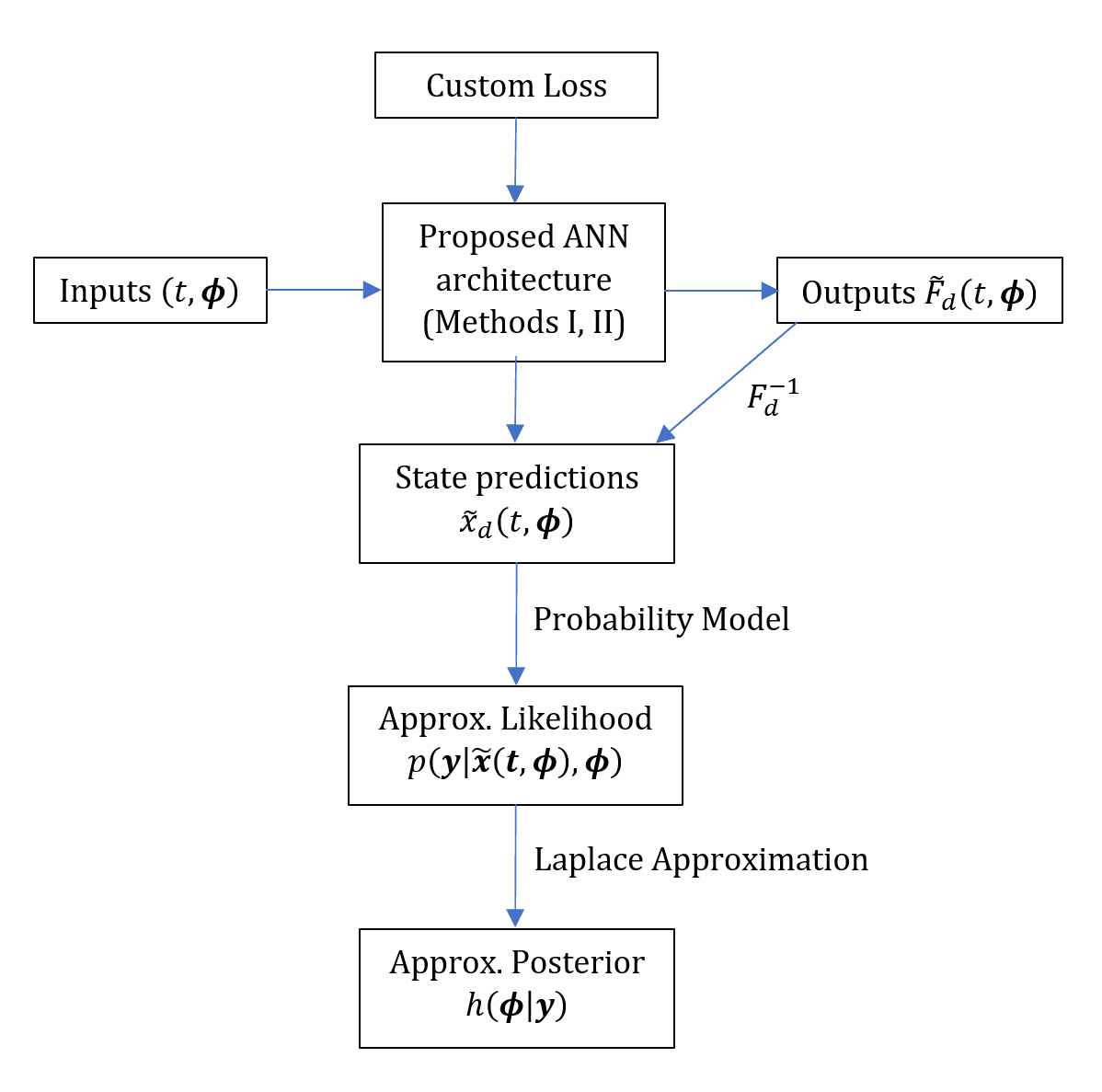
Figure 3 shows a flowchart that summarizes the general algorithm for our methods which can be applied to ODE models arising from various dynamical systems. The next section illustrates the general methodology development for a special ODE model which is the SIR epidemic model.

The SIR model is a compartmental model in epidemiology consisting of three compartments, or states, denoted by Susceptible ($S$), Infectious ($I$) and Removed ($R$). An individual in the population can move from a susceptible state, $S$, to an infectious state, $I$, upon infection, and after a certain infectious period, move to the removed state, $R$; it is assumed that those in the removed state do not return to the susceptible state. We introduce the following notation:

Given these parameters, the SIR ODE model is then specified by the following system of ODEs:

where we have parameterized $c_{I_{0}}:=\ln I(0)$, $c_{\gamma}:=\ln\gamma$ and $c_{\beta}:=\ln\beta$ to ensure that we infer positive values for $\beta,\gamma$ and $I(0)$. Here we assume $\beta$ and $\gamma$ are constant over all $t\in[T_{0},T_{1}]$, as in the original SIR model by Kermack and McKendrick [14]. Thus $\boldsymbol{\phi}=\mathbf{c}:=(c_{I_{0}},c_{\gamma},c_{\beta})$ based on notation introduced in Section 2. Note that $S(0)=P-e^{c_{I_{0}}}$ is not included in $\boldsymbol{\phi}$ since it is simply a function of $c_{I_{0}}$ and $R(0)$ is fixed at 0.

Further differentiating equations (18), (19) and (20) with respect to $c_{I_{0}},c_{\gamma}$ and $c_{\beta}$ extends the ODE system for our methodology’s needs. Abbreviating $S(t,\mathbf{c}),I(t,\mathbf{c})$ and $R(t,\mathbf{c})$ as $S,I$ and $R$ respectively, we derive the following equations.

Applying Method I’s notations to the SIR Model, $\mathbf{x}=(S,I,R)$ and $\mathbf{f}$ is clear from Equations (18) to (20). Equation (21) also gives the constraint $B(\mathbf{x}(t,\mathbf{c}),\mathbf{c})=S(t,\mathbf{c})+I(t,\mathbf{c})+R(t,\mathbf{c})-P=0$. For Method II, $\mathbf{x}^{\dagger}$ is defined as $\Big(S,I,R,\frac{\partial S}{\partial c_{I_{0}}},\frac{\partial I}{\partial c_{I_{0}}},\frac{\partial R}{\partial c_{I_{0}}},\frac{\partial S}{\partial c_{\gamma}},\frac{\partial I}{\partial c_{\gamma}},\frac{\partial R}{\partial c_{\gamma}},\frac{\partial S}{\partial c_{\beta}},\\ \frac{\partial I}{\partial c_{\beta}},\frac{\partial R}{\partial c_{\beta}}\Big)$, and $\mathbf{f}^{\dagger}$ is evident from Equations (18)-(20) and (23)-(31). $\mathbf{B}^{\dagger}(\mathbf{x}^{\dagger}(t,\mathbf{c}),\mathbf{c})$ can similarly be obtained from Equations (32) to (34). With these, we are ready to formulate our ANN architecture, loss functions and training algorithms for the SIR Model.

In order to assess the approximations to the true posterior over a number of experiments, we simulate 200 different sets of data $\{\mathbf{y}_{i}\}_{i=1,2,...,200}$ where each $\mathbf{y}_{i}:=(y_{i}(t_{1}),...,y_{i}(t_{N}))$ is generated from a fixed set of parameters $\mathbf{c}^{*}=(c_{I_{0}}^{*},c_{\gamma}^{*},c_{\beta}^{*})=(\ln 7,\ln 1/7,-0.25)$ (henceforth referred to as the ”true” value of the ODE’s parameters) and $P=10,000$. As in real practice, only some of the $S$-$I$-$R$ compartments will be observed. In this simulated experiment, we choose $y_{i}(t_{n})$ to represent the number of new removed (state $R$) individuals within the time interval $(t_{n-1},t_{n}]$; further setting $t_{n}=n\text{ days}$ means the $y_{i}(t_{n})$’s represent daily numbers of newly removed individuals. Since $\frac{dR}{dt}=e^{c_{\gamma}}I(t,\mathbf{c})$ is the corresponding rate, we may use it as the expected value of $y_{i}(t_{j})$. Hence, for all $i=1,2,...,200$, $y_{i}(t_{n})$ is randomly generated from a Poisson distribution with mean $e^{c_{\gamma}^{*}}I(t_{n},\mathbf{c}^{*})$, where $I(t,\mathbf{c}^{*})$ is the numerical solution of the state $I$ at time $t$ under the parameter setting $\mathbf{c}^{*}$.

References

- [1] Roda WC. Bayesian inference for dynamical systems. Infectious Disease Modelling. 2020;5:221-32. doi:10.1016/j.idm.2019.12.007.
- [2] Chen MH, Shao QM, Ibrahim JG. Monte Carlo methods in Bayesian computation. Springer Science & Business Media; 2012. doi:10.1007/978-1-4612-1276-8.
- [3] Christensen N, Meyer R, Knox L, Luey B. Bayesian methods for cosmological parameter estimation from cosmic microwave background measurements. Classical and Quantum Gravity. 2001;18(14):2677. doi:10.1088/0264-9381/18/14/306.
- [4] Gelman A, Rubin DB. Inference from iterative simulation using multiple sequences. Statistical science. 1992:457-72. doi:10.1214/ss/1177011136.
- [5] Brooks SP, Gelman A. General methods for monitoring convergence of iterative simulations. Journal of computational and graphical statistics. 1998;7(4):434-55. doi:10.2307/1390675.
- [6] Storvik G. Particle filters for state-space models with the presence of unknown static parameters. IEEE Transactions on signal Processing. 2002;50(2):281-9.
- [7] Carvalho CM, Johannes MS, Lopes HF, Polson NG. Particle learning and smoothing. Statistical Science. 2010;25(1):88-106.
- [8] Jiang B, Wu Ty, Zheng C, Wong WH. Learning summary statistic for approximate Bayesian computation via deep neural network. Statistica Sinica. 2017:1595-618.
- [9] Jo H, Son H, Hwang HJ, Jung SY. Analysis of COVID-19 spread in South Korea using the SIR model with time-dependent parameters and deep learning. medRxiv. 2020.
- [10] Jo H, Son H, Hwang HJ, Kim EH. Deep neural network approach to forward-inverse problems. Networks & Heterogeneous Media. 2020;15(2):247.
- [11] Raissi M, Perdikaris P, Karniadakis GE. Physics-informed neural networks: A deep learning framework for solving forward and inverse problems involving nonlinear partial differential equations. Journal of Computational Physics. 2019;378:686-707.
- [12] Ramsay JO, Hooker G, Campbell D, Cao J. Parameter estimation for differential equations: a generalized smoothing approach. Journal of the Royal Statistical Society: Series B (Statistical Methodology). 2007;69(5):741-96.
- [13] Hornik K, Stinchcombe M, White H. Multilayer feedforward networks are universal approximators. Neural networks. 1989;2(5):359-66.
- [14] Kermack WO, McKendrick AG. A contribution to the mathematical theory of epidemics. Proceedings of the royal society of london Series A, Containing papers of a mathematical and physical character. 1927;115(772):700-21.
- [15] Nguyen-Thien T, Tran-Cong T. Approximation of functions and their derivatives: A neural network implementation with applications. Applied Mathematical Modelling. 1999;23(9):687-704.
- [16] McCulloch WS, Pitts W. A logical calculus of the ideas immanent in nervous activity. The bulletin of mathematical biophysics. 1943;5(4):115-33.
- [17] Cybenko G. Approximation by superpositions of a sigmoidal function. Mathematics of control, signals and systems. 1989;2(4):303-14.
- [18] Ferrari S, Stengel RF. Smooth function approximation using neural networks. IEEE Transactions on Neural Networks. 2005;16(1):24-38.
- [19] Adcock B, Dexter N. The gap between theory and practice in function approximation with deep neural networks. SIAM Journal on Mathematics of Data Science. 2021;3(2):624-55.
- [20] Zainuddin Z, Pauline O. Function approximation using artificial neural networks. WSEAS Transactions on Mathematics. 2008;7(6):333-8.
- [21] Yang S, Ting T, Man KL, Guan SU. Investigation of neural networks for function approximation. Procedia Computer Science. 2013;17:586-94.
- [22] Li X. Simultaneous approximations of multivariate functions and their derivatives by neural networks with one hidden layer. Neurocomputing. 1996;12(4):327-43.
- [23] Pukrittayakamee A, Hagan M, Raff L, Bukkapatnam ST, Komanduri R. Practical training framework for fitting a function and its derivatives. IEEE transactions on neural networks. 2011;22(6):936-47.
- [24] Lagaris IE, Likas A, Fotiadis DI. Artificial neural networks for solving ordinary and partial differential equations. IEEE transactions on neural networks. 1998;9(5):987-1000.
- [25] He S, Reif K, Unbehauen R. Multilayer neural networks for solving a class of partial differential equations. Neural networks. 2000;13(3):385-96.
- [26] IEEE. Approximation of a function and its derivatives in feedforward neural networks. vol. 1; 1999.
- [27] Avrutskiy VI. Enhancing Function Approximation Abilities of Neural Networks by Training Derivatives. IEEE transactions on neural networks and learning systems. 2020;32(2):916-24.
- [28] Mai-Duy N, Tran-Cong T. Approximation of function and its derivatives using radial basis function networks. Applied Mathematical Modelling. 2003;27(3):197-220.
- [29] Jianyu L, Siwei L, Yingjian Q, Yaping H. Numerical solution of elliptic partial differential equation using radial basis function neural networks. Neural Networks. 2003;16(5-6):729-34.
- [30] Sarra SA. Adaptive radial basis function methods for time dependent partial differential equations. Applied Numerical Mathematics. 2005;54(1):79-94.
- [31] Gallant AR, White H. On learning the derivatives of an unknown mapping with multilayer feedforward networks. Neural Networks. 1992;5(1):129-38.
- [32] Azevedo-Filho A, Shachter RD. Laplace’s method approximations for probabilistic inference in belief networks with continuous variables. In: Uncertainty Proceedings 1994. Elsevier; 1994. p. 28-36.
- [33] Fletcher R. Practical methods of optimization. John Wiley & Sons; 2013.
- [34] Anonymous. Influenza in a boarding school. British Medical Journal. 1978;1(6112):578.
- [35] Raissi M, Ramezani N, Seshaiyer P. On parameter estimation approaches for predicting disease transmission through optimization, deep learning and statistical inference methods. Letters in Biomathematics. 2019;6(2):1-26.
- [36] Gelman A, Carlin JB, Stern HS, Rubin DB. Bayesian data analysis. Chapman and Hall/CRC; 1995.
- [37] Wand MP, Jones MC. Kernel smoothing. CRC press; 1994.
- [38] Dass SC, Kwok WM, Gibson GJ, Gill BS, Sundram BM, Singh S. A data driven change-point epidemic model for assessing the impact of large gathering and subsequent movement control order on COVID-19 spread in Malaysia. PloS one. 2021;16(5):e0252136.
- [39] Tavaré S, Balding DJ, Griffiths RC, Donnelly P. Inferring coalescence times from DNA sequence data. Genetics. 1997;145(2):505-18.
- [40] Middleton L, Deligiannidis G, Doucet A, Jacob PE. Unbiased Markov chain Monte Carlo for intractable target distributions. Electronic Journal of Statistics. 2020;14(2):2842-91.
- [41] Streftaris G, Gibson GJ. Bayesian inference for stochastic epidemics in closed populations. Statistical Modelling. 2004;4(1):63-75.