Computing a Stable Distance on Merge Trees

Graph-based topological descriptors include merge trees (sometimes specifically referred to as split trees or join trees), Reeb graphs, contour trees, and mapper graphs. Each descriptor is designed to show the changes of the topological structure in the underlying dataset. Reeb graphs are, arguably, the most complex descriptor in this family. Reeb graphs contract each component of each level set into a single point. The contour tree is simply the Reeb graph defined on a simply connected domain – making the contour tree a well-defined tree rather than a directed multigraph. Merge trees are then the simplest (both in structure and in computational cost) of these in that it encodes the sublevel (or superlevel) set topology rather than the levelset topology.

The visualization community has a long history of providing effective computations of these descriptors as well as using them for data analysis. Heine et al. recently surveyed many of their uses [26]. In this section, we highlight some of the more recent works as they relate to applications of level set topology, rather than providing an exhaustive survey. Oesterling et al. construct topological landscapes of high-dimensional point clouds using join trees [30]. Bremer et al. capture the behavior of turbulent mixing by developing hierarchical techniques for merge trees [8]. Thomas et al. explore symmetry detecting using contour trees [39]. Widanagamaachchi et al. study atmospheric phenomena by constructing a tracking on merge trees [42]. Yan et al. compute a structural average of merge trees for understanding statistical properties of collections [44].

Stability of merge trees was proven when the interleaving distance between merge trees was introduced [29]. Afterwards, functional distortion distance was introduced for Reeb graphs [4], the interleaving distance was extended to Reeb graphs [12], and several edit distances were introduced for Reeb graphs [14, 15, 5]. While the Reeb graphs are inherently different summaries of the scalar field, merge trees are still a 1-dimensional graph and thus many of the definitions introduced in these works can be applied directly to merge trees. Researchers have actually shown the equivalence of interleaving, functional distortion, and the universal distance on merge trees [2]. Each of these aforementioned distances have been proven to be both stable and discriminative to the bottleneck distance [12, 14, 15, 7, 5, 29, 4].

Unfortunately, implementations of these distances have been scarce due to their computational complexity. In order to have distances which are practical, other researchers have focused their efforts on defining distances specifically on merge trees due to their simplicity. As stated before, these distances loosen the restriction on either stability or discriminativity in order to have distances which are computationally feasible. To avoid confusion, we will call the collection of distances consisting of the interleaving, functional distortion, and universal distance as the theoretical merge tree distances. We call the collection of distinct distances we discuss below the experimental merge tree distances.

Sridharamurthy et al. introduced an edit distance between merge trees which is experimentally shown to be more discriminative than both the bottleneck and 1-Wasserstein distance [36]. This distance loosens the restriction on stability which makes it computationally feasible. Cases of instability are still addressed by introducing an adjustable parameter which combines saddles which are within the parameters value – simplifying the topology of the merge tree. The distance was also proven to be a well-defined metric on the space of merge trees. This idea was later expanded upon with the introduction of the local merge tree edit distance – a well-defined metric specifically designed to study the local similarities at multiple resolutions rather than providing a global measure [37].

Beketayev et al. provides a computation of a similarity measure for merge trees by first computing all of its branch decomposition trees – data structures which encode features of the merge tree as nodes in a new tree – and then finding pairwise matchings between these trees. The matching imposes a restriction that if $x$ matches to $y$ and $x^{\prime}$ is a child of $x$, then $x^{\prime}$ must be matched to a child of $y$ (or be deleted). This is similar to the ‘ancestor preserving’ restriction imposed by standard tree edit distance (TED) [38]. Our distance that we propose in \autorefsec:distance similarly uses branch decomposition trees in order to encode the feature of a merge tree. We divert from this work by removing the ‘ancestor preserving’ restriction which allows us to maintain stability of our distance.

Saikia et al. [34, 35] produces a similar distance to the one defined by Beketayev et al. They introduce a dynamic programming algorithm to create an extended branch decomposition tree – a data structure which encodes similar data to the conglomerate of all possible branch decomposition trees without having to store all these possibilities in memory. They show the application of this distance on self-similarity of scalar fields and detecting periodicity in time-varying datasets.

To ensure that our resulting structures are well-behaved, we elect to focus our attention towards piecewise linear-scalar fields: scalar fields in which the domain ${\mathbb{X}}$ is triangulable and the function $f$ is piecewise linear. Furthermore, we will focus our work on scalar fields in which the domain is a simply connected, two-dimensional manifold and the function $f$ is a simple Morse function [18]. These conditions ensure that the merge tree is a well-defined, one-dimensional graph [12].

In what follows, we will be working solely with the split tree. Some definitions, theorems, and parts of our algorithm work for both the join and split tree, while others are specific to the split tree due to aspects such as increasing paths from saddle to extrema rather than decreasing paths. However, if we were to negate the original function defined on the scalar field, we can provide a distance for the join tree as well. To this end, we will elect to use the term merge tree and use the notation $\mathcal{M}_{f}$ for a merge tree defined on a scalar field $({\mathbb{X}},f)$.

Since merge trees can be considered as labeled graphs, we will often denote the vertices and edges of $\mathcal{M}_{f}$ as $V(\mathcal{M}_{f})$ and $E(\mathcal{M}_{f})$, respectively. From this, we can define the notion of merge tree isomorphism.

Instead of defining the persistence diagram on the scalar field, we elect to define the persistence diagram by using using the merge tree as a scalar field itself since it reduces the number of classes of points in the persistence diagram and overall makes the comparison between distances on persistence diagrams and distances on merge trees simpler; see Bollen et al.[7] for a discussion on defining the persistence diagram of graph-based descriptors. For the sake of brevity, we show how to construct a persistence diagram from a merge tree and its properties rather than theoretical definitions.

The persistence diagram $\mathrm{Dgm}({\mathcal{M}_{f})}$ of a merge tree $\mathcal{M}_{f}$ is a multiset of points $(a,b)$ which each represent a pair of vertices of the merge tree. These pairs intuitively represent different features of the merge tree. To determine which vertices are paired together, we introduce the elder rule.

Persistence diagrams have been shown to be stable under the well-studied bottleneck distance [10, 11]. The bottleneck distance assign a cost to a matching between the points of two persistence diagrams. We allow for each point to also be matched to an empty node which can be thought of as deleting or inserting that feature.

The branch decomposition tree (BDT) is a data structure which, in topological data analysis, attempts to pair the saddles of contour trees or merge trees to the extrema of that tree. Each node in the BDT would then represent a feature of the original scalar field. Pascucci used the branch decomposition trees to inform a layout for complex contour trees with many self-intersections [31]. Since then, BDTs have seen additional use as representations of merge trees for their comparison [35, 6].

Each merge tree or contour tree has precisely $2^{\frac{n}{2}-1}$ different possible BDTs, where $n$ is the number of nodes [6]. Often, a unique BDT is constructed by weighting the choice of pairing based on a particular measurement – such as persistence of the branch or the number of voxels of the branch in the scalar field [35].

For every hierarchical decomposition of a merge tree $\mathcal{M}_{f}$, we obtain a unique BDT $b_{f}$. Each node $u\in b_{f}$ corresponds to two vertices of $\mathcal{M}_{f}$. If $u\in b_{f}$ is not the root node, then there is a corresponding saddle $u_{s}\in\mathcal{M}_{f}$ and a corresponding maxima $u_{e}\in MM_{f}$. The root node $r\in b_{f}$ corresponds to the global minimum $r_{s}\in\mathcal{M}_{f}$ and a maxima $r_{e}\in\mathcal{M}_{f}$. We denote the set of all possible branch decomposition trees of a merge tree $\mathcal{M}_{f}$ as $\mathcal{B}_{f}$. \autoreffig:mergeTreeToBDT shows the eight different BDTs for a merge tree with eight nodes.

Stability of a distance guarantees that point-wise perturbations introduced into the dataset will not drastically change the merge tree. Saikia et al. [34] defined two different types of instabilities which are exhibited in merge trees: horizontal instabilities and vertical instabilities.

For our algorithm, we will use branch decomposition trees to organize the features of the scalar field. Due to this setup, we may have a situation where a small change in the function values of extrema switches their total ordering – possibly altering the topology of BDTs. This is called a vertical instability. \autoreffig:instabilities depicts the affects of perturbations in a vertical and horizontal manner on a function $f$.

If a similarity measure is strictly bounded below by a baseline distance (up to a constant $c$), then there are cases in which the baseline distance is not able to discern between two merge trees while the distance $d$ does detect some dissimilarity. Furthermore, this implies that if the distance $d$ detects no difference between two merge trees, then the baseline will not detect any difference as well.

A core position on discriminativity being desirable is that we expect these merge tree distances to inherently be more computationally complex than persistence diagram distances since the graph-based descriptors are strictly more complex than set-based descriptors. Thus, these merge tree distances will trade off their computational efficiency for encoding more information in the similarity measure. As with the theoretical merge tree distances, we will use the bottleneck distance as our baseline since the theoretical merge tree distance and bottleneck distance all use a “max-feature-difference” approach to similarity measuring.

A similar notion to discriminativity is isomorphism invariance.

It has been shown that the bottleneck distance is not isomorphism invariant on the space of merge trees while all of the theoretical graph-based distances are [7]. The merge tree edit distance is also isomorphism invariant [36].

The universal distance (originally referred to as the Reeb graph edit distance [5]) is a stable, discriminative distance defined on Reeb graphs and merge trees which has been shown to be the largest stable distance defined on Reeb graphs – a property known as universality. On merge trees, it was shown to be equivalent to the interleaving and functional distortion distance [2] – thus making all of these distances universal.

The universal distance is defined by constructing a zigzag diagram of topological spaces which connects a source merge tree $\mathcal{M}_{f}$ to its target $\mathcal{M}_{g}$. These zigzag diagrams can be intuitively thought of as a sequence of operations carrying one merge tree to another. We use a simplified version of the zigzag diagram for use with our distance. The term carry is used to state that we are transforming a source merge tree $\mathcal{M}_{f}$ into a merge tree $\mathcal{M}^{\prime}$ which is isomorphic to $\mathcal{M}_{g}$.

Each merge tree $\mathcal{M}_{i}\in M$ will have an associated function $f_{i}$. In general, these merge trees need not be Morse. Specifically, we will have merge trees with vertices of degree 4 which is not permitted under the definition of Morse functions on 2-manifolds. The connecting spaces are responsible for changing adjacencies in the merge trees. \autoreffig:zigzagBackForth depicts two different zigzag diagrams. The first carries a merge tree $\mathcal{M}_{f}$ to $\mathcal{M}_{g}$, while the bottom diagram is in reverse order.

When the choice of zigzag diagram is not clear, we use the notation $\mathsf{L}(Z)$ to denote the limit of the zigzag diagram $Z$. See Appendix A.2 for another example of a zigzag diagram with the corresponding spread.

When constructing a distance between merge trees, we need to make sure that the distance captures the difference based on the relationship between features that are in the original scalar field rather than solely on the paired critical points. We encode this hierarchical relationship between features using the BDT, which also captures topological features (pairs of critical points) as individual vertices in the BDT.

Unlike persistence diagrams, there are many different BDTs for each merge tree. Using only one can lead to vertical instabilities in the distance. Thus, in order to adequately find the distance between two merge trees, enumeration of all the BDTs is needed, similar to Beketayev et al. [6]. Let $\mathcal{M}_{f}$, $\mathcal{M}_{g}$ be two merge trees with respective sets of BDTs $\mathcal{B}_{f},\mathcal{B}_{g}$. A matching between a fixed $b_{f}\in\mathcal{B}_{f}$ and $b_{g}\in\mathcal{B}_{g}$ gives us a matching between the features of $\mathcal{M}_{f}$ and $\mathcal{M}_{g}$.

Elements of a matching $M$ fall into three different categories: insertion pairs which have the form $(\lambda,v)$, deletion which pairs have the form $(u,\lambda)$, and relabel pairs which have the form $(u,v)$. If $(u,v)\in M$ and $(u_{p},v_{p})\notin M$, where $u_{p},v_{p}$ are the parents of nodes $u,v$, then $(u,v)$ is further categorized as a movement relabel pair.

An induced zigzag diagram is the zigzag diagram which arises from carrying one merge tree to another. This induced zigzag diagram follows the protocol that we apply insertions, non-movement relabels, movement relabels, and then deletions. We apply insertions first and deletions last since we cannot create disconnected merge trees in our zigzag diagram.

Each matching $M$ between two BDTs $b_{i}\in\mathcal{B}_{f}$,$b_{j}\in\mathcal{B}_{g}$ induces two zigzag diagrams: the forward zigzag diagram $Z_{f,g}$ from $\mathcal{M}_{f}$ to $\mathcal{M}_{g}$, and the backward zigzag diagram $Z_{g,f}$ from $\mathcal{M}_{g}$ to $\mathcal{M}_{f}$. The difference in these two induced zigzag diagrams is when the relabel pairs are applied. Taking the minimum cost over the forward and backward zigzag diagram ensures that we handle the instability in a way that keeps the distance below the $L_{\infty}$ distance. \autoreffig:zigzagBackForth depicts an example of the possible difference. Since these merge trees are horizontal $\varepsilon$-unstable, we need to make sure that our distance is less than or equal to $\varepsilon$ for us to have a distance below the $L^{\infty}$ distance. In this case, $\varepsilon=|\tilde{g}(y_{1})-\tilde{g}(y_{2})|$. Note that the backward zigzag diagram has a spread less than $\varepsilon$.

We define the cost of a matching as follows:

Suppose we have a merge tree $\mathcal{M}_{f}$. As an example, we describe how to construct a persistence-based BDT. We first take the global min $v_{0}$ and find the path $p_{v_{0},v_{n}}$ to the global max $v_{n}$. The pair $(v_{0},v_{n})$ is placed as the root of the BDT. For every vertex $v$ along this path, we recursively call the construction of the BDT algorithm with $v$ being the new root. Each node $v\in p_{v_{0},v_{n}}$ contributes a single child node to the root node. The algorithm ends when all nodes are paired.

For general BDTs, we must consider every maxima $v$ that is in the up-path of a root $u$ as a possible pairing rather than just the global maxima of that branch. In order to avoid redundant computations of the same branches, we add another recursive layer to the BDT algorithm.

Suppose that $(v_{s},v_{e})$ is a pair corresponding to a branch $\mathsf{B}$ which has just been placed into a BDT $b$. For computation of a single BDT, we would recursively call this operation for all $v\in p_{v_{s},v_{e}}$. However, we know that for every node $(v_{s},v_{e})$, there are multiple different configurations of its children. To avoid redundant computations, we generate a specific number of BDTs for each possible pairing of a saddle $v$, for each $v\in p_{v_{s},v_{e}}$. First, assume $v$ is the only vertex in $p_{v_{s},v_{e}}$ which is not one of the endpoints. Let $\{u_{1},\ldots,u_{m}\}$ be the set of extrema in the up-path of $v$. For each pair $(v,u_{i})$, we construct a new copy of $b$ and add $(v,u_{i})$ as the child of $(v_{s},v_{e})$.

Now, suppose instead that $\{v_{1},\ldots,v_{k}\}$ is the set of vertices in $p_{v_{s},v_{e}}$ which are not the endpoints. We proceed to carry out the same step as if there was only one non-endpoint vertex $v$, except instead of making $m$ copies of $b$, we need to make a copy for the possible combinations of choices of extrema pairing for all $v_{i}\in\{v_{1},\ldots,v_{k}\}$. More specifically, if $m_{i}$ denotes the number of extrema that $v_{i}$ can be paired with, we make $m_{1}\cdot m_{2}\cdot\ldots\cdot m_{k-1}\cdot m_{k}$ copies of $b$. Each $b$ gets a unique set of nodes added as the children of $(v_{s},v_{e})$.

The A* algorithm maintains a priority queue $Q$ which holds a list of partial matchings $M^{\prime}$ with a current cost $c(M^{\prime})$. Since our distance requires the full matching before a true cost can be determined, we use the bottleneck distance between the currently matched nodes in order to under approximate cost. More specifically, let $P$ be a partial matching between $b_{f}$ and $b_{g}$. Then $c(M^{\prime})=\max_{(u,v)\in M^{\prime}}c(u,v)$, where $c(u,v)$ is the cost function in \autorefdef:bottleneckDistance. As stated earlier, providing an under approximation to the true cost will guarantee that we still reach an optimal solution. However, since our under approximation will not necessarily converge to the true cost when we reach a full matching (unlike standard GED), we have to have an additional step which computes the true cost of the matching and to determine whether to continue finding better matchings dependent on this cost. Appendix A.3 shows an overview of our A* algorithm with this additional module.

The efficiency of A* is heavily dictated by introducing pruning techniques to reduce the number of possible matchings and using a good heuristic function which approximates the future cost along a particular path in the search tree. In our case, we can effectively prune the search space by not matching two nodes to one another if it would be cheaper to simply insert or delete both the nodes. As for a heuristic function, we introduce the function $h(M^{\prime})$ which finds the lowest possible future cost based on the fact that if $b_{f}$ has $n$ unmatched nodes and $b_{g}$ has $m$ unmatched nodes, we must insert or delete the difference in the number of nodes. See Appendix A.1 for more information on our pruning and heuristic function. As opposed to GED, our “approximate cost” would then be $\max\{c(M^{\prime}),h(M^{\prime})\}$ rather than $c(M^{\prime})+h(M^{\prime})$.

Let $b_{f}$ and $b_{g}$ be the branch decomposition trees that we are comparing and let $M$ be the current full matching between them. As stated before, the forward zigzag diagram $Z_{f,g}$ is constructed by applying insertions, non-movement relabels, movement relabels, and then deletions to $b_{f}$ which ultimately creates $b_{g}$. Just as the graph edit distance can be thought of as constructing edit sequences to carry one graph to another, our distance can be thought of as altering the branch decomposition $b_{f}$ with this set of operations in order to construct $b_{g}$.

There is a one-to-one mapping between the vertices of any two connecting spaces. Thus, we keep the labeling of each connecting space the same. When we say that $x_{i}=x_{j}$ for two vertices in different connecting spaces, this implies that $i=j$. We denote the set of vertices in the connecting spaces as $V(X)$.

Let $x^{i},x^{i+1}$ be vertices of $X_{i},X_{i+1}$, respectively. Note that $x_{i}=\{x_{i}^{1},\ldots,x_{i}^{n-1}\}$ is an element of $\mathsf{L}(Z)$ for all $x_{i}\in V(X)$. Additional elements are added if $q_{i,i+1}(x^{i})=q_{i+1,i+1}(x^{i+1})$, for some $x^{i}\in X_{i}$ and $x^{i+1}\in X_{i+1}$ where $x^{i}\neq x^{i+1}$. We call these swaps. For example, Fig. 4 has a swap in both the forward and backward zigzag diagram. For the forward zigzag diagram, a swap occurs in $\mathcal{M}_{3}$ where $q_{1,2}(x_{1})=q_{2,2}(x_{2})$. This implies $\{x_{1},x_{1},x_{2}\}$ is also an element of the limit. For every swap, there are two options to continue constructing the limit: continue with the same vertex or move to the swapped vertex.

In what follows, each pair $(u,v)\in M$ would create at least one connecting space and one merge tree. If $(u,v)$ is a movement relabel, we may create more. Each time we would create a merge tree and connecting space, instead we create a copy the previous BDT and alter it according to the pair (inserting a node, deleting a node, relabeling, or moving a node). By the end of the algorithm, we are left with a set of BDTs $\{b_{f}=b_{1},b_{2},\ldots,b_{m-1},b_{m}=b_{g}\}$ and a list $S$ of length $m$ which will contain our swaps. These two data structures are enough to determine the elements of $\mathsf{L}(Z)$.

To begin, we construct a copy of $b_{f}$ and apply all $n$ insertions. We sort the list of insertions by increasing depth order to make sure that if $u$ is to be inserted on $u^{\prime}$, then $u^{\prime}$ already exists. Non-movement relabels are then conducted in no particular order.

Let $b_{k}$ be the current BDT. In a movement relabel, we have a source branch $u\in b_{k}$, its parent $u_{p}\in b_{k}$, a target branch $v\in b_{g}$ and the parent of the target $v_{p}\in b_{g}$. Let $u^{\prime}$ be such that $(u^{\prime},v)\in M$ and $u^{\prime}_{p}$ be such that $(u^{\prime}_{p},v_{p})\in M$. Our goal is then to move $u$ to have parent $u^{\prime}_{p}$. We find the path $\rho:u_{p}\rightsquigarrow u^{\prime}_{p}$. The node closest to the root of $b_{k}$ in depth is known as the intersection. The intersection is the branch where $u$ does not need to attach to its saddle. For every other branch $w$ in the path $\rho$, we know we must add an additional connecting space and add the swap tuple $(u_{s},w_{s})$, where $u_{s}$ and $w_{s}$ are saddles of the respective merge trees, to the list. \autoreffig:movementExample depicts an example of recording the intersection and swaps for moving a branch.

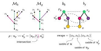
Movement relabels need to be conducted in an order that makes sure that the BDT stays connected. Our A* algorithm has the restriction that if $u$ is an ancestor of $u^{\prime}$, then $u$ cannot become a descendant of $u^{\prime}$ since it is suboptimal (i.e. another choice of BDT should be used if this is the case). However, once we begin altering the original BDT, there are situations where this $u$ needs to be moved onto its parent. To alleviate this, we maintain another priority queue which holds all the movements, first ranked by the depth to the root. If we were to apply a movement, we check if this disconnection will occur. If so, we push the movement pair back into this priority queue with a lower priority index and move onto the next movement.

Algorithm 1 shows the pseudocode of how we first choose pairs of branch decomposition trees and then subsequently feed these pairs into our A* algorithm. Note that we introduce a “cutoff” variable which indicates when to stop the A* computation of a pair of BDTs. If the cheapest current matching is ever larger than this cutoff, we stop the computation and move onto the next pair.

We took the TOSCA non-rigid world dataset, which contains a collection of shapes of animals and humans in different poses, and then we computed the average geodesic distance on each of them using the method suggested by Hilaga et al. [27]. We randomly sampled a subset of 100 vertices from each mesh, calculated the geodesic distance from every vertex to the subset and then took the average. Next we persistence simplified the data, by using a custom threshold for each mesh so that we get 14 nodes in the split tree. The largest persistence simplification value was 7.34 which implies that the distances we have computed are at most 3.67 above the true distance.

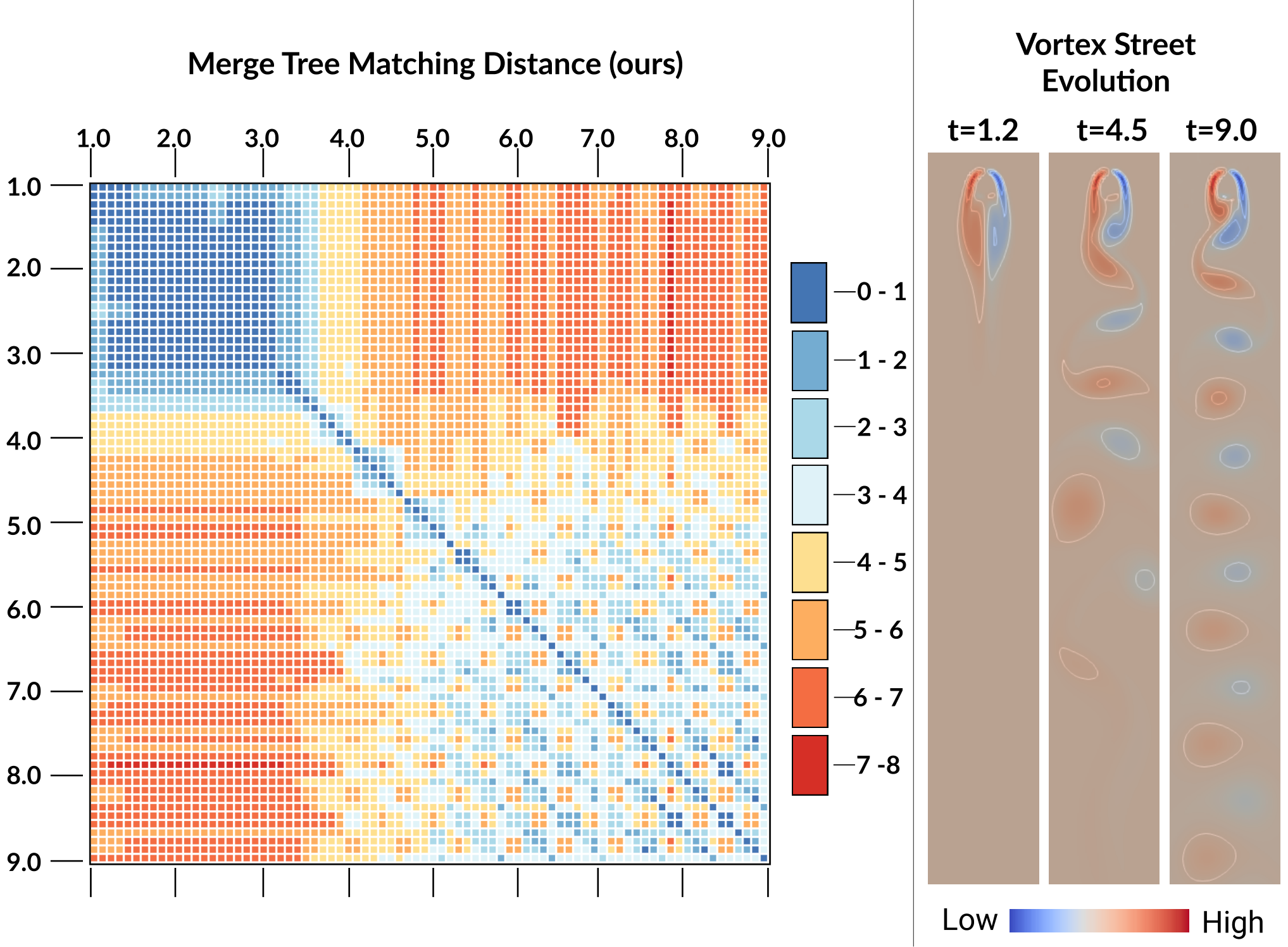
We obtained a von Kármán Vortex Street dataset from [23] and calculated the vorticity scalar field for a set of uniformly sampled timesteps. Then we persistence simplified each timestep so that the resulting merge would have exactly 14 nodes. Since we were only planning on obtaining 14 nodes, we decided to clip the vortex data so that more information from the clipped timestep could be obtained. Then we computed the pairwise distance using our distance between time-steps. The distance matrix is shown in \autoreffig:vortexDistMatrix. The largest persistence simplification value was 6.60, which implies that the distances we have computed are 3.30 above the true distance.

To test the stability of our distance, we constructed a baseline scalar field $({\mathbb{X}}_{0},f_{0})$ with three maxima, two saddles, and the global minimum. The two connected saddles are within $\varepsilon$ of each other – making the scalar field horizontally $\varepsilon$-unstable. We generated 36 new scalar fields by applying a random plane multiplied by a Gaussian, to simulate random noise. The bottleneck, merge tree matching, and $L^{\infty}$ distance was computed for each scalar field when compared to the baseline and plotted in \autoreffig:teaser. We found that, as desired, our distance lay between the bottleneck and $L^{\infty}$ distance.

The perturbation was chosen with several specifics in mind in order to correctly mimic the case of horizontal stability. Let $\varepsilon=|\tilde{f}(x_{2})-\tilde{f}(x_{1})|$. The extrema $x_{3},x_{4},x_{5}$ are assigned function values such that each are more than $2\varepsilon$ greater than their connected saddle. Otherwise, the perturbation which we apply would create a new scalar field $({\mathbb{X}},\tilde{g})$ such that deletion of $e(x_{2},x_{4})$, inserting $e(y_{2},x_{4})$, and adjusting the function value of $x_{1}$ to be the function value of $y_{1}$ would be optimal. Furthermore, since we wanted to focus on horizontal instabilities in this experiment, we made sure that the difference between $x_{5}$ and $x_{3}$ is larger than $\varepsilon$. Otherwise, the perturbation would essentially just be “reflecting” the merge tree, i.e. mapping $x_{3}$ to $y_{5}$ and $x_{5}$ to $y_{3}$.

It is worth noting that if there was no topology change in the data and our perturbation was only causing differences in function value, then our merge tree matching distance would be equal to the bottleneck distance. Thus, this distance is sufficiently capturing a perturbation which changes the topology of the merge tree.