跳到论文正文
W Papers独立论文阅读器 arXiv:2210.08591 论文正文 计算阅读时间 · 0%
引用这篇论文根据当前论文元数据生成,正式投稿前建议核对。


License: CC BY 4.0
arXiv:2210.08591v4 [math.PR] 16 Nov 2023
\DefineSimpleKey

bibarxiveprint \DefineSimpleKeybibarxivid \DefineSimpleKeybibarxivclass

Importance Sampling for the Empirical Measure of Weakly Interacting DiffusionsThanks: Z.W.B. was partially supported by the National Science Foundation (DMS 2107856). The majority of this work was completed while Z.W.B. was a PhD candidate at Boston University. M.H. was partially supported by NSF-DMS 1902854, ARO W911NF-20-1-0244, and a subgrant of NSF-OAC 2139536. The authors of the paper would like to thank both reviewers for a their careful and constructive reviews of this article.

Z.W. Bezemek Email address, Zachary William Bezemek : zwb@duke.edu Zachary William BezemekDuke University, Department of Mathematics
120 Science Drive, Durham, NC 27708, USA
and M. Heldman Email address, Max Heldman : maxh@vt.edu Max HeldmanVirginia Tech, Department of Mathematics
225 Stanger Street, Blacksburg, VA 24061, USA
Date: August 11, 2026
Abstract.

We construct an importance sampling method for computing statistics related to rare events for weakly interacting diffusions. Standard Monte Carlo methods behave exponentially poorly with the number of particles in the system for such problems. Our scheme is based on subsolutions of a Hamilton-Jacobi-Bellman (HJB) equation on Wasserstein space which arises in the theory of mean-field (McKean-Vlasov) control. We identify conditions under which such a scheme is asymptotically optimal. In the process, we make connections between the large deviations principle for the empirical measure of weakly interacting diffusions, mean-field control, and the HJB equation on Wasserstein space. We also provide evidence, both analytical and numerical, that with sufficient regularity of the HJB equation, our scheme can have vanishingly small relative error in the many particle limit.

Key words and phrases: 
interacting particle systems, empirical measure, large deviations, importance sampling
2010 Mathematics Subject Classification
60F10, 60F05, 65C05

1. Introduction

Consider the weakly interacting particle system:

(1) d​Xti,N,s,y\displaystyle dX^{i,N,s,y}_{t} =b⁡(Xti,N,s,y,μtN,s,y)​d​t+σ⁡(Xti,N,s,y,μtN,s,y)​d​Wti,Xsi,N,s,y=yi\displaystyle=b(X^{i,N,s,y}_{t},\mu^{N,s,y}_{t})dt+\sigma(X^{i,N,s,y}_{t},\mu^{N,s,y}_{t})dW^{i}_{t},\quad X^{i,N,s,y}_{s}=y_{i}

on some stochastic basis (Ω,ℱ,ℙ),{ℱt}t∈[s,T](\Omega,\mathcal{F},\mathbb{P}),\{\mathcal{F}_{t}\}_{t\in[s,T]} satisfying the usual conditions, where b:ℝd×𝒫2​(ℝd)→ℝdb\mathrel{\mathop{\ordinarycolon}}\mathbb{R}^{d}\times\mathcal{P}_{2}(\mathbb{R}^{d})\rightarrow\mathbb{R}^{d}, σ:ℝd×𝒫2​(ℝd)→ℝd×m\sigma\mathrel{\mathop{\ordinarycolon}}\mathbb{R}^{d}\times\mathcal{P}_{2}(\mathbb{R}^{d})\rightarrow\mathbb{R}^{d\times m}, {Wi}i∈ℕ\{W^{i}\}_{i\in\mathbb{N}} are independent mm-dimensional standard ℱt\mathcal{F}_{t}-Brownian motions initialized at Wsi=0W^{i}_{s}=0, i∈{1,…,N}i\in\{1,...,N\}. Here 𝒫2​(ℝd)\mathcal{P}_{2}(\mathbb{R}^{d}) is the space of probability measures with finite second moment (see Definition A.1). In (1), NN denotes the total number of particles, i∈{1,2,…,N}i\in\{1,2,...,N\} indexes a particular particle, and μN,s,y∈C⁡([0,T],𝒫⁡(ℝd))\mu^{N,s,y}\in C([0,T];\mathcal{P}(\mathbb{R}^{d})) is the empirical measure:

(2) μtN,s,y≔1N​∑i=1NδXti,N,s,y,t∈[s,T].\displaystyle\mu^{N,s,y}_{t}\coloneqq\frac{1}{N}\sum_{i=1}^{N}\delta_{X^{i,N,s,y}_{t}},\quad t\in[s,T].

The ii’th entry of the vector y=(y1,y2,…)∈⊕i=1∞ℝdy=(y_{1},y_{2},...)\in\oplus_{i=1}^{\infty}\mathbb{R}^{d} contains the deterministic initial condition for the ii’th particle at time ss satisfying 0≤s≤t≤T0\leq s\leq t\leq T. The entries yiy_{i} for i>Ni>N are ignored for any particular value of NN; we include them in defining (1) for convenience, since our purpose will be to consider the sequence of solutions to (1) as N→∞N\to\infty. We will at times identify yy with its projection onto ℝd​N=[ℝd]N=⊕i=1Nℝd\mathbb{R}^{dN}=[\mathbb{R}^{d}]^{N}=\oplus_{i=1}^{N}\mathbb{R}^{d} without ambiguity.

In this paper, we design a control-based importance sampling scheme for estimating functionals of the form

(3) 𝔼⁡[exp⁡(−N​G​(μTN,s,y))],G:𝒫⁡(ℝd)→ℝ.\displaystyle\mathbb{E}\biggl[\exp\left(-NG(\mu^{N,s,y}_{T})\right)\biggr],\quad G\mathrel{\mathop{\ordinarycolon}}\mathcal{P}(\mathbb{R}^{d})\rightarrow\mathbb{R}.

The basic method goes as follows: letting viN:[s,T]×ℝd​N→ℝmv^{N}_{i}\mathrel{\mathop{\ordinarycolon}}[s,T]\times\mathbb{R}^{dN}\rightarrow\mathbb{R}^{m} be a chosen bounded function, or control, for each i∈{1,…,N}i\in\{1,...,N\} and N∈ℕN\in\mathbb{N}, we consider the controlled version of the interacting particle system (1) given by

(4) d​X^ti,N,s,y=[b⁡(X^ti,N,s,y,μ^ti,N,s,y)+σ⁡(X^ti,N,s,y,μ^ti,N,s,y)​viN​(t,X^t1,N,s,y,…,X^tN,N,s,y)]​d​t+σ⁡(X^ti,N,s,y,μ^ti,N,s,y)​d​W^ti,X^si,N,s,y=yi.\begin{split}d\hat{X}^{i,N,s,y}_{t}&=[b(\hat{X}^{i,N,s,y}_{t},\hat{\mu}^{i,N,s,y}_{t})+\sigma(\hat{X}^{i,N,s,y}_{t},\hat{\mu}^{i,N,s,y}_{t})v^{N}_{i}(t,\hat{X}^{1,N,s,y}_{t},...,\hat{X}^{N,N,s,y}_{t})]dt\\ &+\sigma(\hat{X}^{i,N,s,y}_{t},\hat{\mu}^{i,N,s,y}_{t})d\hat{W}^{i}_{t},\quad\hat{X}^{i,N,s,y}_{s}=y_{i}.\end{split}

Girsanov’s theorem allows us to convert statistics for the controlled system (4) into statistics for (1); therefore, in order to develop a more accurate Monte Carlo estimator for (1) our objective will be to identify controls viNv_{i}^{N} that reduce the variance of our target statistic compared with the uncontrolled version, or in the best case cause the relative variance to vanish as N→∞N\rightarrow\infty. By these measures, we find that subsolutions of a zero-viscosity Hamilton-Jacobi-Bellman (HJB) equation on Wasserstein space, which we derive starting with the Dawson-Gärtner large deviations principle (LDP) [19, 5], provide controls with good performance.

Our main results, stated rigorously in Section 2, show that under certain assumptions our scheme outperforms standard Monte Carlo methods by requiring a subexponential number of samples to achieve a given relative error in estimating (3) as N→∞N\rightarrow\infty (Theorem 2.4). Under stronger assumptions, we show that in fact only a vanishing number of simulations suffices (Theorem 2.5), so that for large NN our method requires only a single sample. Our theoretical results are confirmed by numerical experiments in Section 4.

Our importance sampling scheme is related to and inspired by previous work concerning the development of asymptotically optimal importance sampling methods for estimating expectations of the form

(5) 𝔼⁡[exp⁡(−1ϵ​G​(XTϵ,s,y))],G∈Cb​(ℝd),\displaystyle\mathbb{E}\biggl[\exp\left(-\frac{1}{\epsilon}G\left(X^{\epsilon,s,y}_{T}\right)\right)\biggr],\quad G\in C_{b}(\mathbb{R}^{d}),

where Xϵ,s,yX^{\epsilon,s,y} is a single particle satisfying, e.g., the small-noise SDE:

(6) d​Xtϵ,s,y=b⁡(Xtϵ,s,y)​d​t+ϵ​σ​(Xtϵ,s,y)​d​Wt,Xsϵ,s,y=y∈ℝd.\begin{split}dX^{\epsilon,s,y}_{t}&=b(X^{\epsilon,s,y}_{t})dt+\sqrt{\epsilon}\sigma(X^{\epsilon,s,y}_{t})dW_{t},\\ X^{\epsilon,s,y}_{s}&=y\in\mathbb{R}^{d}.\end{split}

We will draw parallels between the small-noise setting and ours throughout this article.

A general strategy for efficiently computing (5) involves exploiting the connection between the large deviations rate function of Freidlin-Wentzell (FW) [41] and a class of first-order Hamilton-Jacobi-Bellman (HJB) equations, whose subsolutions can then be leveraged to obtain optimal controls for the zero-noise process X0,s,yX^{0,s,y}. In turn, the controls can be used to design an optimal change of measure for estimating (5). The control formulation of the FW rate function, provided via the weak convergence approach to large deviations of Dupuis and Ellis [18, 4], makes the chain linking the rate function, zero-viscosity HJB equation, and optimal control of the zero-noise process more evident. The strategy described above has been applied for a diverse range of stochastic models [35, 76, 37, 38, 70].

Elevating the above framework for small-noise SDE importance sampling schemes to interacting particle systems is a major contribution of this paper. Moreover, the connections between the approaches used herein and in the small-noise setting allow us to conjecture (see Remark 2.6) about extending this research to problems related to metastable dynamics that have been previously considered for the small-noise case (see, e.g., [71] and the references therein) such as exit probabilities and mean first passage times. We therefore view this paper as the first step towards a new method of designing importance sampling schemes for studying properties of the empirical measure which are of interest to the greater scientific community, such as the free-energy differences for chemical and biological molecular systems [10, 45, 75, 47] or exit times of the empirical measure from domains of attraction in models related to social dynamics and consensus convergence [17, 42, 43, 32, 46].

Let us now make the comparison between the interacting particle system (1) and the small-noise system (6) more explicit. It is well known that μN,s,y→ℒ⁡(Xs,ν)\mu^{N,s,y}\rightarrow\mathcal{L}(X^{s,\nu}) in distribution when considered as 𝒫⁡(C⁡([s,T],ℝd))\mathcal{P}(C([s,T];\mathbb{R}^{d}))-valued random variables. Here ν∈𝒫⁡(ℝd)\nu\in\mathcal{P}(\mathbb{R}^{d}) is the weak limit as N→∞N\rightarrow\infty of the empirical measures 1N​∑i=1Nδyi\frac{1}{N}\sum_{i=1}^{N}\delta_{y_{i}}, and Xs,νX^{s,\nu} satisfies the McKean-Vlasov equation:

(7) d​Xts,ν\displaystyle dX^{s,\nu}_{t} =b⁡(Xts,ν,ℒ⁡(Xts,ν))​d​t+σ⁡(Xs,ν,ℒ⁡(Xts,ν))​d​Wt,Xss,ν∼ν.\displaystyle=b(X^{s,\nu}_{t},\mathcal{L}(X^{s,\nu}_{t}))dt+\sigma(X^{s,\nu},\mathcal{L}(X^{s,\nu}_{t}))dW_{t},\quad X^{s,\nu}_{s}\sim\nu.

This phenomenon, known as the propagation of chaos, goes back to the works of Kac [51]. The empirical measure μN,s,y\mu^{N,s,y} can also formally be seen to satisfy an infinite-dimensional small-noise equation, analogous to (6), with parameter ϵ=1N\epsilon=\frac{1}{\sqrt{N}}, as per pp. 249-250 of [19]. Thus, the problem of estimating (3) has the same basic structure as the more well-known problem of estimating (5), but with a different state space.

An LDP for the many-particle limit of {μN,s,y}N∈ℕ\{\mu^{N,s,y}\}_{N\in\mathbb{N}} was first established in the classical work of [19] in the case where the diffusion coefficient σ\sigma does not depend on the empirical measure, with the result extended via the weak convergence approach of Dupuis and Ellis [18] to the general setting in [5]. In the latter, the form of the rate function is given in terms of a control problem (see Theorem 1.2), which further motivates our search for an asymptotically optimal importance sampling scheme for (3) associated with an HJB equation as in the small-noise SDE setting. In contrast to the setting of small-noise SDEs, where the state space of the HJB equation is Euclidean space, we find that the appropriate HJB equation to consider in our setting of measure-valued random variables is posed on Wasserstein space.

Perhaps due to the computational intractability of both the Dawson-Gärtner [19] and Budhiraja-Dupuis-Fischer [5] rate functions, practical applications of the LDP for the many-particle limit of the empirical measure (2) associated with (1) have been few and far between (for some exceptions see, e.g., [42, 43, 61, 20]). On the other hand, in recent years the HJB equation on Wasserstein space of [65] (along with the related equations in [54, 14]) has received an immense amount of attention both in terms of numerical applications [16, 28, 78, 55, 58, 25, 48] and theoretical results [7, 15, 65, 62, 63, 64, 77, 27, 66]. The Dawson-Gärtner rate function has previously been related to the theory of mean field games and control through the observation that it can be viewed in terms of derivatives of the free energy associated to the limiting McKean-Vlasov equation viewed as a gradient flow on Wasserstein space in some settings [1, 2, 44, 56, 52, 60, 59, 53]. However, to our knowledge, this paper is the first time that the connection between the LDP rate function (10) and the HJB equation on Wasserstein space (23) has been made explicit in the literature (see Remark 2.2).

As far as we are aware, this paper also represents the first time the problem of estimating (3) with an asymptotically optimal importance sampling scheme has been considered, though many other versions of the small-noise importance sampling problem have appeared in the literature. These include, for example, discrete-time Markov chains [37, 38], diffusions with multiscale structure [35, 29], and stochastic partial differential equations [40, 23]. See in addition [49, 67, 36, 39, 71, 76] for a diverse, but by no means comprehensive, collection of small-noise importance sampling research in a variety of settings. We in particular mention the work of [31] on the design of importance sampling schemes for small-noise McKean-Vlasov SDEs using a decoupling approach (see also [8, 9]) and a complete change of measure approach. The problem posed in [31] is significantly different from the one we consider here, principally because they seek to estimate statistics of the limiting McKean-Vlasov equation (7) rather than the interacting particle system (1). The change of measure they employ is therefore based on the Freidlin-Wentzell (small-noise) LDP for Brownian motion, rather than the Sanov-type (many-particle) LDP for the empirical measure (2) used in our setting. Note that Freidlin-Wentzell LDPs have been derived in different settings for McKean-Vlasov equations [21, 57], though they were not directly employed in the results of [31, 8, 9].

Finally, we note that methods of importance sampling for high-dimensional diffusions have also been established in previous research, e.g., [67, 69, 73]). While in theory these could be applied to estimate (3), they are designed for more general problems than ours and therefore do not exploit the exchangeability of the particles, and resulting propagation of chaos, to obtain an asymptotically optimal scheme. However, it may be that a combination of these non-asymptotic techniques with ours could allow us to treat a broader range of problems in the future, as we remark in Section 6.

The rest of the paper is organized as follows. We establish notation in Subsection 1.1 below, and go on to provide background on large deviations theory for the empirical measure in Subsection 1.2. Then, in Subsection 1.3 we develop measures of performance for the control-based importance sampling of diffusions for computing statistics of the form (3), some of which can be quantified using large deviations theory. In Section 2, we formally derive the HJB Equation on Wasserstein space and state our main results, Theorem 2.4 and Theorem 2.5. In Section 3, we introduce a class of linear-quadratic examples for which the HJB equation can be solved analytically and discuss simple cases in which our scheme can be thoroughly analyzed in comparison to standard Monte Carlo, along the way comparing with results for small-noise diffusion processes on ℝd\mathbb{R}^{d}. In Section 4, we demonstrate our method with numerical examples. Section 5 contains detailed proofs of the results stated in Section 2, before Section 6 provides concluding remarks. Lastly, in Appendix A we provide additional background on the calculus of square-integrable probability measures, 𝒫2​(ℝd)\mathcal{P}_{2}(\mathbb{R}^{d}).

1.1. Notation

In the following paragraph, let 𝑿\bm{X} and 𝒀\bm{Y} be Polish spaces, and (Ω,ℱ,μ)(\Omega,\mathcal{F},\mu) a measure space. In the course of this paper, we denote by 𝒫⁡(𝑿)\mathcal{P}(\bm{X}) the space of probability measures on 𝑿\bm{X} endowed with the topology of weak convergence. We use 𝒫2​(𝑿)⊂𝒫​(𝑿)\mathcal{P}_{2}(\bm{X})\subset\mathcal{P}(\bm{X}) to denote the subspace of 𝒫⁡(𝑿)\mathcal{P}(\bm{X}) consisting of square-integrable probability measures on 𝑿\bm{X} endowed with the 2-Wasserstein metric (see Definition A.1). We additionally let ℬ⁡(𝑿)\mathcal{B}(\bm{X}) be the Borel σ\sigma-algebra associated with 𝑿\bm{X}, C⁡(𝑿,𝒀)C(\bm{X};\bm{Y}) the space of continuous functions from 𝑿\bm{X} to 𝒀\bm{Y}, Cb​(𝑿)C_{b}(\bm{X}) the space of bounded, continuous functions from 𝑿\bm{X} to ℝ\mathbb{R} with norm ‖ϕ‖∞≔supx∈𝑿|ϕ⁡(x)|\mathinner{\!\left\lVert\phi\right\rVert}_{\infty}\coloneqq\sup_{x\in\bm{X}}|\phi(x)|, and for p≥1p\geq 1 we define Lp​(Ω,ℱ,μ,ℝd)L^{p}(\Omega,\mathcal{F},\mu;\mathbb{R}^{d}) as the space of pp-integrable functions on (Ω,ℱ,μ)(\Omega,\mathcal{F},\mu) with values in ℝd\mathbb{R}^{d} and norm

‖ϕ‖Lp​(Ω,ℱ,μ,ℝd)=(∫Ω|ϕ⁡(z)|p​μ​(𝑑z))1/p.\mathinner{\!\left\lVert\phi\right\rVert}_{L^{p}(\Omega,\mathcal{F},\mu;\mathbb{R}^{d})}=\biggl(\int_{\Omega}|\phi(z)|^{p}\mu(dz)\biggr)^{1/p}.

Cb,L​(ℝd)⊂Cb​(ℝd)C_{b,L}(\mathbb{R}^{d})\subset C_{b}(\mathbb{R}^{d}) is the set of bounded, globally Lipschitz functions ϕ:ℝd→ℝ\phi\mathrel{\mathop{\ordinarycolon}}\mathbb{R}^{d}\rightarrow\mathbb{R} with norm ‖ϕ‖b,L≔‖ϕ‖∞+supx,y∈ℝd,x≠y|ϕ⁡(x)−ϕ⁡(y)||x−y|\mathinner{\!\left\lVert\phi\right\rVert}_{b,L}\coloneqq\mathinner{\!\left\lVert\phi\right\rVert}_{\infty}+\sup_{x,y\in\mathbb{R}^{d},x\neq y}\frac{|\phi(x)-\phi(y)|}{|x-y|}. For ϕ∈L1​(𝑿,μ),μ∈𝒫⁡(𝑿)\phi\in L^{1}(\bm{X},\mu),\mu\in\mathcal{P}(\bm{X}), we define the pairing ⟨ϕ,μ⟩\langle\phi,\mu\rangle by

⟨ϕ,μ⟩≔∫𝑿ϕ⁡(x)​μ​(𝑑x).\langle\phi,\mu\rangle\coloneqq\int_{\bm{X}}\phi(x)\mu(dx).

We note that, as in the above definitions, the codomain for a given function space is assumed to be ℝ\mathbb{R} unless otherwise specified. We will also occasionally refer to a measure on a topological space 𝑿\bm{X} without explicitly stating the corresponding σ\sigma-algebra; in this case, the measurable sets are assumed to come from ℬ⁡(𝑿)\mathcal{B}(\bm{X}).

Partial derivatives of a function ϕ\phi with respect to a variable xx are normally denoted by ∂xϕ\partial_{x}\phi; if the variable xx is measure valued then the derivative ∂x\partial_{x} should be interpreted in the Lions sense (see Appendix A). For time derivatives ∂tϕ\partial_{t}\phi with respect to t∈I⊆ℝ+t\in I\subseteq\mathbb{R}^{+}, we also use the notation ϕ˙\dot{\phi}.

For ϕ:[0,T]×𝒫2​(ℝd)→ℝ\phi\mathrel{\mathop{\ordinarycolon}}[0,T]\times\mathcal{P}_{2}(\mathbb{R}^{d})\rightarrow\mathbb{R}, we use ϕ∈C1,2​([0,T]×𝒫2​(ℝd))\phi\in C^{1,2}([0,T]\times\mathcal{P}_{2}(\mathbb{R}^{d})) to mean that μ↦ϕ⁡(t,μ)\mu\mapsto\phi(t,\mu) is fully C2C^{2} in the sense of Definition A.2 for all tt, with all derivatives in that definition jointly continuous in (t,z,z′,μ)(t,z,z^{\prime},\mu) and the map t↦ϕ⁡(t,μ)t\mapsto\phi(t,\mu) continuously differentiable in tt. The subspace Cb1,2​([0,T]×𝒫2​(ℝd))⊂C1,2​([0,T]×𝒫2​(ℝd))C_{b}^{1,2}([0,T]\times\mathcal{P}_{2}(\mathbb{R}^{d}))\subset C^{1,2}([0,T]\times\mathcal{P}_{2}(\mathbb{R}^{d})) denotes the class of functions ϕ\phi such that further ϕ\phi and all its derivatives from Definition A.2 are uniformly bounded.

For x,y∈ℝdx,y\in\mathbb{R}^{d}, x=(x1,…,xd),y=(y1,…,yd)x=(x_{1},...,x_{d}),y=(y_{1},...,y_{d}), x⋅yx\cdot y denotes the standard inner product x⋅y≔∑i=1dxi​yix\cdot y\coloneqq\sum_{i=1}^{d}x_{i}y_{i}. For A,B∈ℝd×dA,B\in\mathbb{R}^{d\times d} matrices with entries {ai​j}i,j=1d\{a_{ij}\}_{i,j=1}^{d} and {bi​j}i,j=1d\{b_{ij}\}_{i,j=1}^{d} respectively, A:B≔∑i,j=1dai​j​bi​jA\mathrel{\mathop{\ordinarycolon}}B\coloneqq\sum_{i,j=1}^{d}a_{ij}b_{ij}.

For x∈⊕i=1Nℝdx\in\oplus_{i=1}^{N}\mathbb{R}^{d} or ⊕i=1∞ℝd\oplus_{i=1}^{\infty}\mathbb{R}^{d}, we will denote by μxN\mu^{N}_{x} associated empirical measure, i.e., the element of 𝒫⁡(ℝd)\mathcal{P}(\mathbb{R}^{d}) given by

μxN≔1N​∑i=1Nδxi.\displaystyle\mu^{N}_{x}\coloneqq\frac{1}{N}\sum_{i=1}^{N}\delta_{x_{i}}.

Finally, for given sequences {fn},{gn}\{f_{n}\},\{g_{n}\} in ℝ+\mathbb{R}^{+}, we use the following notation to compare their asymptotic behavior: fn=𝒪⁡(gn)f_{n}=\mathcal{O}(g_{n}) if there is a constant C>0C>0 independent of nn such that fn≤C​gnf_{n}\leq Cg_{n}, and fn=o⁡(gn)f_{n}=o(g_{n}) if fngn→0\frac{f_{n}}{g_{n}}\to 0 as n→∞n\to\infty. If instead of positive real numbers fnf_{n} and gng_{n} are sequences on normed spaces, we use the same notation to refer to the behavior of the sequences |fn||f_{n}| and |gn||g_{n}|.

1.2. Large deviations results and an HJB equation for the particle system

We now introduce some of the key tools for proving the our main results in Section 2, namely, a stochastic control representation for the LDP associated with the empirical measure (2) as provided by [5] and a control representation for statistics of the form (3). The final tool, the HJB equation on Wasserstein space, will be introduced in Section 2.

The Laplace principle stated in Theorem 1.2 is based on the controlled version of (7):

(8) d​X^tv,s,ν=[b⁡(X^tv,s,ν,ℒ⁡(X^tv,s,ν))+σ⁡(X^tv,s,ν,ℒ⁡(X^tv,s,ν))​v​(t)]​d​t+σ⁡(X^tv,s,ν,ℒ⁡(X^tv,s,ν))​d​Wt,X^sv,s,ν∼ν.\begin{split}d\hat{X}^{v,s,\nu}_{t}&=[b(\hat{X}^{v,s,\nu}_{t},\mathcal{L}(\hat{X}^{v,s,\nu}_{t}))+\sigma(\hat{X}^{v,s,\nu}_{t},\mathcal{L}(\hat{X}^{v,s,\nu}_{t}))v(t)]dt+\sigma(\hat{X}^{v,s,\nu}_{t},\mathcal{L}(\hat{X}^{v,s,\nu}_{t}))dW_{t},\\ \hat{X}^{v,s,\nu}_{s}&\sim\nu.\end{split}

For the LDP to hold, we need the following assumptions on the particle system (1), the controlled version of the limiting McKean-Vlasov equation (8), and the problem data:

Assumption 1.1.

Suppose:

  1. (A1)

    The initial conditions yy for (1) are such that there exists ν∈𝒫2​(ℝd)\nu\in\mathcal{P}_{2}(\mathbb{R}^{d}) with μyN→ν\mu^{N}_{y}\rightarrow\nu as N→∞N\rightarrow\infty.

  2. (A2)

    The coefficients bb and σ\sigma are continuous on ℝd×𝒫⁡(ℝd).\mathbb{R}^{d}\times\mathcal{P}(\mathbb{R}^{d}).

  3. (A3)

    For all N∈ℕN\in\mathbb{N}, existence and uniqueness of solutions holds in the strong sense for the system of SDEs (1).

  4. (A4)

    Weak uniqueness holds for solutions of (8) in the sense that if Θ1,Θ2\Theta^{1},\Theta^{2} are probability measures such that for i=1,2i=1,2:

    • •

      Θi\Theta^{i} is the law of some process triple (X^vi,s,ν,vi,Wi)(\hat{X}^{v_{i},s,\nu},v_{i},W^{i}) satisfying (8) on some filtered probability space (Ωi,ℱi,ℙi),{ℱti}t∈[s,T](\Omega^{i},\mathcal{F}^{i},\mathbb{P}^{i}),\{\mathcal{F}^{i}_{t}\}_{t\in[s,T]} satisfying the usual conditions

    • •

      viv_{i} is an ℱti\mathcal{F}^{i}_{t}-progressively measurable control with 𝔼Θi​[∫sT|vi​(t)|2​𝑑t]<∞\mathbb{E}^{\Theta^{i}}\left[\int_{s}^{T}|v_{i}(t)|^{2}dt\right]<\infty

    • •

      WiW^{i} a standard ℱti\mathcal{F}^{i}_{t}-Brownian motion with Wsi=0W^{i}_{s}=0

    and Θ1∘ϑ−1=Θ2∘ϑ−1\Theta^{1}\circ\vartheta^{-1}=\Theta^{2}\circ\vartheta^{-1} where ϑ\vartheta is the identity mapping in the second and third coordinates and the evaluation map at time ss in the first coordinate, then Θ1=Θ2\Theta^{1}=\Theta^{2}.

  5. (A5)

    For any sequence of controlled processes {X^i,N,s,y}\{\hat{X}^{i,N,s,y}\} from (4) with ℱt\mathcal{F}_{t}-progressively measurable controls vN=(v1N,…,vNN)v^{N}=(v^{N}_{1},...,v^{N}_{N}) satisfying

    supN∈ℕ𝔼⁡[1N​∑i=1N∫sT|viN​(t)|2​𝑑t]<∞,\sup_{N\in\mathbb{N}}\mathbb{E}\left[\frac{1}{N}\sum_{i=1}^{N}\int_{s}^{T}|v^{N}_{i}(t)|^{2}dt\right]<\infty,

    μ^N≔1N​∑i=1NδX^i,N,s,y\hat{\mu}^{N}\coloneqq\frac{1}{N}\sum_{i=1}^{N}\delta_{\hat{X}^{i,N,s,y}} is tight as a sequence of 𝒫⁡(C⁡([s,T],ℝd))\mathcal{P}(C([s,T];\mathbb{R}^{d}))-valued random variables.

Assumption 1.1 is taken directly from [5] with the exception of (A4), which is a mildly less restrictive form of weak uniqueness under which the arguments from [5] still hold (see Lemma 3.4 in [3] or Definition 3.6 in [11]). For verifiable conditions on the data of the problem under which (A4) holds, from Appendix C in [22] we have that:

  1. (A1’)

    b,σb,\sigma are jointly globally Lipschitz on ℝd×𝒫⁡(ℝd)\mathbb{R}^{d}\times\mathcal{P}(\mathbb{R}^{d}) where 𝒫⁡(ℝd)\mathcal{P}(\mathbb{R}^{d}) is equipped with the bounded Lipschitz metric dB​L(μ,ν)≔sup{ϕ∈Cb,L(ℝd):‖ϕ‖b,L≤1}∫ℝdϕ(x)[μ(dx)−ν(dx)]d_{BL}(\mu,\nu)\coloneqq\sup_{\{\phi\in C_{b,L}(\mathbb{R}^{d})\mathrel{\mathop{\ordinarycolon}}\mathinner{\!\left\lVert\phi\right\rVert}_{b,L}\leq 1\}}\int_{\mathbb{R}^{d}}\phi(x)[\mu(dx)-\nu(dx)].

  2. (A2’)

    σ\sigma is bounded and σ⁡(x,μ)=σ⁡(μ)\sigma(x,\mu)=\sigma(\mu).

are enough to imply (A2)-(A5). Note that the proof given in [22] that (A1’) and (A2’) together imply (A4) (Proposition C.1 in [22]), is based on an erroneous localization argument. See [3] for a correct proof.

We are now ready to state the LDP for the empirical measure.

Theorem 1.2.

Under Assumption 1.1, for any F∈Cb​(C⁡([s,T],𝒫⁡(ℝd)))F\in C_{b}(C([s,T];\mathcal{P}(\mathbb{R}^{d}))):

(9) limN→∞−1Nlog𝔼[exp(−NF(μN,s,y))]=𝒢(s,ν;F)≔infμ∈C⁡([s,T],𝒫⁡(ℝd)){Ss,Tν(μ)+F(μ)},\displaystyle\lim_{N\rightarrow\infty}-\frac{1}{N}\log\mathbb{E}\left[\exp(-NF(\mu^{N,s,y}))\right]=\mathcal{G}(s,\nu;F)\coloneqq\inf_{\mu\in C([s,T];\mathcal{P}(\mathbb{R}^{d}))}\left\{S^{\nu}_{s,T}(\mu)+F(\mu)\right\},

where Ss,Tν:C⁡([s,T],𝒫⁡(ℝd))→[0,+∞]S^{\nu}_{s,T}\mathrel{\mathop{\ordinarycolon}}C([s,T];\mathcal{P}(\mathbb{R}^{d}))\rightarrow[0,+\infty] is given by

(10) Ss,Tν(μ)≔infv∈𝒰:μ⁡(t)=ℒ⁡(X^tv,s,ν),t∈[s,T]12𝔼[∫sT|v(t)|2dt].\displaystyle S^{\nu}_{s,T}(\mu)\coloneqq\inf_{v\in\mathcal{U}\mathrel{\mathop{\ordinarycolon}}\mu(t)=\mathcal{L}(\hat{X}^{v,s,\nu}_{t}),t\in[s,T]}\frac{1}{2}\mathbb{E}\left[\int_{s}^{T}|v(t)|^{2}dt\right].

In the above we take inf∅=+∞\inf\emptyset=+\infty, and in the expression for Ss,Tν​(μ)S^{\nu}_{s,T}(\mu) the admissible set of controls 𝒰\mathcal{U} is the set of all quadruples ((Ω,ℱ,ℙ),{ℱt}t∈[s,T],v,W)((\Omega,\mathcal{F},\mathbb{P}),\{\mathcal{F}_{t}\}_{t\in[s,T]},v,W) such that:

  • 1.

    ((Ω,ℱ,ℙ),{ℱt})((\Omega,\mathcal{F},\mathbb{P}),\{\mathcal{F}_{t}\}) forms a stochastic basis satisfying the usual conditions,

  • 2.

    WW is a standard mm-dimensional Brownian motion initialized at Ws=0W_{s}=0,

  • 3.

    vv is an ℝm\mathbb{R}^{m}-valued {ℱt}\{\mathcal{F}_{t}\}-progressively measurable process such that 𝔼⁡[∫sT|v⁡(t)|2​𝑑t]<∞\mathbb{E}\left[\int_{s}^{T}|v(t)|^{2}dt\right]<\infty.

We write v∈𝒰v\in\mathcal{U} to denote ((Ω,ℱ,ℙ),{ℱt}t∈[s,T],v,W)∈𝒰((\Omega,\mathcal{F},\mathbb{P}),\{\mathcal{F}_{t}\}_{t\in[s,T]},v,W)\in\mathcal{U} in the above. For each v∈𝒰v\in\mathcal{U}, X^tv,ν\hat{X}^{v,\nu}_{t} satisfies the controlled McKean-Vlasov equation (8) on the space (Ω,ℱ,ℙ),{ℱt}t∈[s,T](\Omega,\mathcal{F},\mathbb{P}),\{\mathcal{F}_{t}\}_{t\in[s,T]} with driving Brownian motion WW.

Proof.

The result follows from Theorem 3.1 in [5] (see also Theorem 5.1 in [22]) by applying the contraction principle to pose the rate function on C⁡([s,T],𝒫⁡(ℝd))C([s,T];\mathcal{P}(\mathbb{R}^{d})) rather than 𝒫⁡(C⁡([s,T],ℝd))\mathcal{P}(C([s,T];\mathbb{R}^{d})) as in Proposition 5.6 of [11]. ∎

The following corollary of Theorem 3.6 in [4], which provides a prelimit expression for the left-hand side of (9) which can be applied to prove Theorem 1.2, is also critical to our arguments in this paper. In Section 5, we apply it to several auxiliary systems of the form (1) with different choices of the drift term in the course of proving Theorem 2.4. The drift terms in the new system have a slightly different form from those in (1), since they are allowed here to directly depend on the time variable.

To distinguish these auxiliary systems and their solutions from those of the original system (1), we establish alternative notation here for the solutions of the controlled and uncontrolled auxiliary systems and their empirical measures that we will also use in Section 5.

Proposition 1.3.

Let μ~tN,s,y=1N​∑i=1NδX~ti,N,s,y,t∈[s,T]\tilde{\mu}^{N,s,y}_{t}=\frac{1}{N}\sum_{i=1}^{N}\delta_{\tilde{X}^{i,N,s,y}_{t}},t\in[s,T] where X~ti,N,s,y\tilde{X}^{i,N,s,y}_{t} solves the system (11) (i.e., (1) with bb replaced by b~\tilde{b}):

(11) d​X~ti,N,s,y\displaystyle d\tilde{X}^{i,N,s,y}_{t} =b~​(t,X~ti,N,s,y,μ~tN,s,y)​d​t+σ⁡(X~ti,N,s,y,μ~tN,s,y)​d​W~ti,X~si,N,s,y=yi\displaystyle=\tilde{b}(t,\tilde{X}^{i,N,s,y}_{t},\tilde{\mu}^{N,s,y}_{t})dt+\sigma(\tilde{X}^{i,N,s,y}_{t},\tilde{\mu}^{N,s,y}_{t})d\tilde{W}^{i}_{t},\quad\tilde{X}^{i,N,s,y}_{s}=y_{i}

and b~,σ\tilde{b},\sigma are such that existence and uniqueness holds in the strong sense for the system of SDEs (11) and W~i\tilde{W}^{i} are IID standard mm-dimensional Brownian motions initialized at W~si=0\tilde{W}^{i}_{s}=0. Then for F∈Cb​(C⁡([s,T],𝒫⁡(ℝd)))F\in C_{b}\left(C([s,T];\mathcal{P}(\mathbb{R}^{d}))\right):

(12) −1N​log⁡𝔼⁡[exp⁡(−N​F​(μ~N,s,y))]=infuN∈𝒰N{𝔼⁡[12​N​∑i=1N∫sT|uiN​(t)|2​𝑑t]+𝔼⁡[F⁡(μ¯N,s,y)]},\displaystyle-\frac{1}{N}\log\mathbb{E}\left[\exp(-NF(\tilde{\mu}^{N,s,y}))\right]=\inf_{u^{N}\in\mathcal{U}^{N}}\left\{\mathbb{E}\left[\frac{1}{2N}\sum_{i=1}^{N}\int_{s}^{T}|u^{N}_{i}(t)|^{2}dt\right]+\mathbb{E}[F(\bar{\mu}^{N,s,y})]\right\},

where 𝒰N\mathcal{U}^{N} is the space of adapted controls uN=(u1N,…,uNN),uiN:[s,T]→ℝmu^{N}=(u^{N}_{1},...,u^{N}_{N}),u^{N}_{i}\mathrel{\mathop{\ordinarycolon}}[s,T]\rightarrow\mathbb{R}^{m} such that 𝔼⁡[∫sT|uN​(t)|2​𝑑t]<∞\mathbb{E}\left[\int_{s}^{T}|u^{N}(t)|^{2}dt\right]<\infty, and μ¯N,s,y\bar{\mu}^{N,s,y} is the empirical measure associated with the controlled version of (11), i.e.,

d​X¯ti,N,s,y\displaystyle d\bar{X}^{i,N,s,y}_{t} =b~​(t,X¯ti,N,s,y,μ¯tN,s,y)​d​t+σ⁡(X¯ti,N,s,y,μ¯tN,s,y)​u​(t)​d​t+σ⁡(X¯ti,N,s,y,μ¯tN,s,y)​d​W~ti,X¯si,N,s,y=yi.\displaystyle=\tilde{b}(t,\bar{X}^{i,N,s,y}_{t},\bar{\mu}^{N,s,y}_{t})dt+\sigma(\bar{X}^{i,N,s,y}_{t},\bar{\mu}^{N,s,y}_{t})u(t)dt+\sigma(\bar{X}^{i,N,s,y}_{t},\bar{\mu}^{N,s,y}_{t})d\tilde{W}^{i}_{t},\quad\bar{X}^{i,N,s,y}_{s}=y_{i}.

1.3. Log-efficiency and asymptotic optimality in control-based importance sampling

Recall our definition of the controlled particle system (4), and let

(13) Zi,N,s,y≔exp(−∫sTviN(t,X^ti,N,s,y,…,X^ti,N,s,y)⋅dW^ti−12∫sT|viN(t,X^ti,N,s,y,…,X^ti,N,s,y)|2dt).\displaystyle Z^{i,N,s,y}\coloneqq\exp\biggl(-\int_{s}^{T}v^{N}_{i}(t,\hat{X}^{i,N,s,y}_{t},...,\hat{X}^{i,N,s,y}_{t})\cdot d\hat{W}^{i}_{t}-\frac{1}{2}\int_{s}^{T}|v^{N}_{i}(t,\hat{X}^{i,N,s,y}_{t},...,\hat{X}^{i,N,s,y}_{t})|^{2}dt\biggr).

By Girsanov’s theorem, an unbiased estimator for (3) is given by

(14) δ^N≔1M​∑j=1Mexp⁡(−N​G​(μ^N,s,y,j))​∏i=1NZi,N,s,y,j\displaystyle\hat{\delta}_{N}\coloneqq\frac{1}{M}\sum_{j=1}^{M}\exp\left(-NG(\hat{\mu}^{N,s,y,j})\right)\prod_{i=1}^{N}Z^{i,N,s,y,j}

where (μ^N,s,y,j,Z1,N,s,y,j,…,ZN,N,s,y,j)(\hat{\mu}^{N,s,y,j},Z^{1,N,s,y,j},...,Z^{N,N,s,y,j}) are MM independent samples of (μ^N,s,y,Z1,N,s,y​…,ZN,N,s,y)(\hat{\mu}^{N,s,y},Z^{1,N,s,y}...,Z^{N,N,s,y}), and

(15) μ^ti,N,s,y≔1N​∑i=1NδX^ti,N,s,y.\displaystyle\hat{\mu}^{i,N,s,y}_{t}\coloneqq\frac{1}{N}\sum_{i=1}^{N}\delta_{\hat{X}^{i,N,s,y}_{t}}.

We note that the standard Monte Carlo method estimator, which we denote by δN\delta_{N}, corresponds to (14) with viN=0v_{i}^{N}=0, so that Zi,N,s,y,j≡1Z^{i,N,s,y,j}\equiv 1.

We define the relative error of the estimator (14) by

(16) ρ⁡(δ^N)=1M​𝔼​δ^N2−[𝔼​δ^N]2[𝔼​δ^N]2=1M​𝔼⁡[exp⁡(−2​N​G​(μ^N,s,y))​∏i=1N(Zi,N,s,y)2]𝔼​[exp⁡(−N​G​(μN,s,y))]2−1.\displaystyle\rho(\hat{\delta}_{N})=\frac{1}{\sqrt{M}}\sqrt{\frac{\mathbb{E}\hat{\delta}_{N}^{2}-\left[\mathbb{E}\hat{\delta}_{N}\right]^{2}}{\left[\mathbb{E}\hat{\delta}_{N}\right]^{2}}}=\frac{1}{\sqrt{M}}\sqrt{\frac{\mathbb{E}\biggl[\exp(-2NG(\hat{\mu}^{N,s,y}))\prod_{i=1}^{N}(Z^{i,N,s,y})^{2}\biggr]}{\mathbb{E}\biggl[\exp(-NG(\mu^{N,s,y}))\biggr]^{2}}-1}.

To control the size of (16) we either need to increase the number of samples MM or reduce the variance by choosing viNv_{i}^{N} so that

(17) R⁡(δ^N)≔𝔼⁡[exp⁡(−2​N​G​(μ^N,s,y))​∏i=1N(Zi,N,s,y)2]𝔼​[exp⁡(−N​G​(μN,s,y))]2,\displaystyle R(\hat{\delta}_{N})\coloneqq\frac{\mathbb{E}\biggl[\exp(-2NG(\hat{\mu}^{N,s,y}))\prod_{i=1}^{N}(Z^{i,N,s,y})^{2}\biggr]}{\mathbb{E}\biggl[\exp(-NG(\mu^{N,s,y}))\biggr]^{2}},

is close to 1. With this in mind, we define our first measure of the efficiency for an importance sampling scheme (14) in terms of the asymptotic behavior of R⁡(δ^N)R(\hat{\delta}_{N}) as N→∞N\rightarrow\infty:

Definition 1.4.

An importance sampling scheme of the form (14) is called log-efficient if

limN→∞−1NlogR(δ^N)=0.\displaystyle\lim_{N\rightarrow\infty}-\frac{1}{N}\log R(\hat{\delta}_{N})=0.

Note that, in our definition, we do not require that R⁡(δ^N)→1R(\hat{\delta}_{N})\to 1 or even R⁡(δ^N)=𝒪⁡(1)R(\hat{\delta}_{N})=\mathcal{O}(1); instead we only ask that as N→∞N\rightarrow\infty, R⁡(δ^N)R(\hat{\delta}_{N}) does not grow exponentially in NN.

The notion of log-efficiency can also be described in terms of large deviations theory. For the uncontrolled system, from (9) in Theorem 1.2 we know that if G∈Cb​(𝒫⁡(ℝd))G\in C_{b}(\mathcal{P}(\mathbb{R}^{d})) and Assumption 1.1 holds, then

(18) limN→∞1N​log⁡𝔼⁡[exp⁡(−N​G​(μTN,s,y))]=−𝒢(s,ν;μ↦G(μT))≔−γ1,limN→∞1N​log⁡𝔼⁡[exp⁡(−2​N​G​(μTN,s,y))]=−𝒢(s,ν;μ↦2G(μT))≔−γ2.\begin{split}\lim_{N\rightarrow\infty}\frac{1}{N}\log\mathbb{E}[\exp(-NG(\mu^{N,s,y}_{T}))]&=-\mathcal{G}(s,\nu;\mu\mapsto G(\mu_{T}))\coloneqq-\gamma_{1},\\ \lim_{N\rightarrow\infty}\frac{1}{N}\log\mathbb{E}[\exp(-2NG(\mu^{N,s,y}_{T}))]&=-\mathcal{G}(s,\nu;\mu\mapsto 2G(\mu_{T}))\coloneqq-\gamma_{2}.\end{split}

Thus, for the standard Monte Carlo scheme the relative error can be written in terms of γ1\gamma_{1} and γ2\gamma_{2} as follows:

(19) ρ⁡(δN)=1M​exp⁡(N⁡[2​γ1−γ2+o⁡(1)])−1\displaystyle\rho(\delta_{N})=\frac{1}{\sqrt{M}}\sqrt{\exp(N[2\gamma_{1}-\gamma_{2}+o(1)])-1}

Starting from the inequality 𝔼[exp(−2NG(μTN,s,y)]≥𝔼[exp(−NG(μTN)]2\mathbb{E}[\exp(-2NG(\mu^{N,s,y}_{T})]\geq\mathbb{E}[\exp(-NG(\mu^{N}_{T})]^{2}, taking logarithms, multiplying by −1N-\frac{1}{N}, and taking the limit N→∞N\rightarrow\infty shows that γ2≤2​γ1.\gamma_{2}\leq 2\gamma_{1}. Evidently, the relative error ρ⁡(δN)\rho(\delta_{N}) grows exponentially in NN if the inequality is strict, i.e., γ:=2​γ1−γ2>0\gamma\mathrel{\mathop{\ordinarycolon}}=2\gamma_{1}-\gamma_{2}>0. Exponentially many samples are therefore required to reduce the relative error below a given tolerance in that case.

Now, we assume that the the relative error for the importance sampling scheme (16) admits the same representation as the standard Monte Carlo importance sampling scheme in (19), with analogous quantities γ^1\hat{\gamma}_{1}, γ^2\hat{\gamma}_{2}, and γ^=2​γ^1−γ^2\hat{\gamma}=2\hat{\gamma}_{1}-\hat{\gamma}_{2}. That is:

(20) ρ⁡(δ^N)=1M​exp⁡(N⁡[γ^+o⁡(1)])−1.\displaystyle\rho(\hat{\delta}_{N})=\frac{1}{\sqrt{M}}\sqrt{\exp(N[\hat{\gamma}+o(1)])-1}.

Note that in the same way as with standard Monte Carlo, we can conclude via Jensen’s inequality that γ^≥0\hat{\gamma}\geq 0. Then we can compare the relative error ρ⁡(δ^N)\rho(\hat{\delta}_{N}) to the Monte Carlo relative error ρ⁡(δN)\rho(\delta_{N}) by comparing the corresponding quantities γ^\hat{\gamma} and γ\gamma:

  1. 1.

    If γ^<γ\hat{\gamma}<\gamma, then the importance sampling scheme is more efficient than standard Monte Carlo in the sense that asymptotically (as N→∞N\rightarrow\infty), it yields a smaller relative error.

  2. 2.

    If γ^=0\hat{\gamma}=0, then the importance sampling scheme is log-efficient and, if γ>0\gamma>0,

    ρ⁡(δ^N)=1M​exp⁡(o⁡(N))−1=o⁡(ρ⁡(δN)).\rho(\hat{\delta}_{N})=\frac{1}{\sqrt{M}}\sqrt{\exp(o(N))-1}=o(\rho\left(\delta_{N}\right)).

The object of our first result Theorem 2.4 presented in the next section is to show conditions under which, for our choice of controls, γ^<γ\hat{\gamma}<\gamma or γ^=0\hat{\gamma}=0.

Though the assumptions underlying Theorem 2.4 preclude the relative error of our importance sampling scheme from growing exponentially, extremely fast subexponential growth rates may still be possible. To obtain a more refined result, one needs to study the behavior of the o⁡(1)o(1) terms in R⁡(δ^N)R(\hat{\delta}_{N}). To that end, our second main result, Theorem 2.5, assumes an expansion of the prelimit quantities on the left-hand side of (18) leading to an expression for R⁡(δ^N)R(\hat{\delta}_{N}) of the form

(21) R⁡(δ^N)=exp⁡(a0​N+a1+a2​N−1+…).\displaystyle R(\hat{\delta}_{N})=\exp\left(a_{0}N+a_{1}+a_{2}N^{-1}+...\right).

Note that here a0a_{0} plays the same role as γ^\hat{\gamma} in (20). Analysis of the coefficients in the power series appearing in the exponential shows that, under stronger regularity assumptions than required for our Theorem 2.4, a0=a1=0a_{0}=a_{1}=0, which implies that the importance sampling scheme has vanishing relative error:

Definition 1.5.

An estimator of the form (14) is said to have vanishing relative error if, for ρ⁡(δ^N)\rho(\hat{\delta}_{N}) as in (16),

limN→∞ρ⁡(δ^N)=0.\displaystyle\lim_{N\rightarrow\infty}\rho(\hat{\delta}_{N})=0.

We conclude this chapter by comparing to the small-noise diffusion regime. Our discussion in this section parallels that of the first section in [76], in which similar importance sampling scheme for small-noise diffusions is presented along with numerical schemes for estimating the optimal controls. However, we note that in our paper stating the LDP and its underlying assumptions is somewhat more involved due to the measure-valued state space.

In [76], the authors also provide sufficient conditions for a log-efficient importance sampling scheme for small-noise diffusions to have vanishing relative error. For our Theorem 2.5, we instead opt to perform an analysis in the spirit of the later [72]. The paper [72] furthered the analysis of the small-noise case by expanding the o⁡(1)o(1) terms in the relative error into powers of the small-noise parameter ϵ\epsilon to recover log-efficiency from the first-order expansion, and the vanishing relative error result from of [76] from the second-order expansion (see also the related Section 3 of [68]).

2. The HJB Equation and Statement of Main Results

We now turn to the full statement of our importance sampling scheme in terms of the solution to an HJB equation on Wasserstein space, explain its relationship to the rate function (10), and give a formal derivation of the importance sampling scheme and the HJB equation as the zero viscosity limit of a sequence of zero variance controls.

Starting with the Hamiltonian function which acts on μ∈𝒫2​(ℝd)\mu\in\mathcal{P}_{2}(\mathbb{R}^{d}), p:ℝd→ℝdp\mathrel{\mathop{\ordinarycolon}}\mathbb{R}^{d}\rightarrow\mathbb{R}^{d} and Γ:ℝd→ℝd×d\Gamma\mathrel{\mathop{\ordinarycolon}}\mathbb{R}^{d}\rightarrow\mathbb{R}^{d\times d} by:

(22) H0​(μ,p,Γ)\displaystyle H_{0}(\mu,p,\Gamma) =−∫ℝdb(x,μ)⋅p(x)−12p(x)⋅[σσ⊤(x,μ)p(x)]+12σσ⊤(x,μ):Γ(x)μ(dx),\displaystyle=-\int_{\mathbb{R}^{d}}b(x,\mu)\cdot p(x)-\frac{1}{2}p(x)\cdot[\sigma\sigma^{\top}(x,\mu)p(x)]+\frac{1}{2}\sigma\sigma^{\top}(x,\mu)\mathrel{\mathop{\ordinarycolon}}\Gamma(x)\mu(dx),

the HJB equation on Wasserstein space is given by:

(23) −∂tΨ(t,ν)+H0(ν,∂μΨ(t,ν)[⋅],∂z∂μΨ(t,ν)[⋅])=0,t∈[0,T),ν∈𝒫2(ℝd),Ψ⁡(T,ν)=G(ν),ν∈𝒫2(ℝd).\begin{split}-\partial_{t}\Psi(t,\nu)+H_{0}(\nu,\partial_{\mu}\Psi(t,\nu)[\cdot],\partial_{z}\partial_{\mu}\Psi(t,\nu)[\cdot])&=0,\qquad t\in[0,T),\nu\in\mathcal{P}_{2}(\mathbb{R}^{d}),\\ \Psi(T,\nu)&=G(\nu),\qquad\nu\in\mathcal{P}_{2}(\mathbb{R}^{d}).\end{split}

Recall here that ∂μΨ⁡(t,ν)​[⋅]:ℝd→ℝd\partial_{\mu}\Psi(t,\nu)[\cdot]\mathrel{\mathop{\ordinarycolon}}\mathbb{R}^{d}\rightarrow\mathbb{R}^{d}, the derivative of Ψ\Psi in the measure-valued variable μ\mu, denotes the Lions derivative of Ψ\Psi at ν\nu (Definition A.1 in Appendix A).

We will make use of the following notion of subsolutions to (23):

Definition 2.1.

We call Ψ:[0,T]×𝒫2​(ℝd)→ℝ\Psi\mathrel{\mathop{\ordinarycolon}}[0,T]\times\mathcal{P}_{2}(\mathbb{R}^{d})\rightarrow\mathbb{R} a classical subsolution to (23) if:

  1. (i)

    Ψ∈C1,2​([0,T]×𝒫2​(ℝd))\Psi\in C^{1,2}([0,T]\times\mathcal{P}_{2}(\mathbb{R}^{d}))

  2. (ii)

    ∂tΨ⁡(t,μ)−H0​(μ,∂μΨ⁡(t,μ)​[⋅],∂z∂μΨ⁡(t,μ)​[⋅])≥0\partial_{t}\Psi(t,\mu)-H_{0}(\mu,\partial_{\mu}\Psi(t,\mu)[\cdot],\partial_{z}\partial_{\mu}\Psi(t,\mu)[\cdot])\geq 0 for all t∈[0,T),μ∈𝒫2​(ℝd)t\in[0,T),\mu\in\mathcal{P}_{2}(\mathbb{R}^{d})

  3. (iii)

    Ψ⁡(T,μ)≤G⁡(μ),μ∈𝒫2​(ℝd)\Psi(T,\mu)\leq G(\mu),\mu\in\mathcal{P}_{2}(\mathbb{R}^{d})

  4. (iv)

    There exists C>0C>0 such that

    supt∈[0,T],μ∈𝒫2​(ℝd),z∈ℝd|∂μΨ⁡(t,μ)​[z]|\displaystyle\sup_{t\in[0,T],\mu\in\mathcal{P}_{2}(\mathbb{R}^{d}),z\in\mathbb{R}^{d}}|\partial_{\mu}\Psi(t,\mu)[z]| ≤C,\displaystyle\leq C,
    supt∈[0,T],μ∈𝒫2​(ℝd)|∂z∂μΨ⁡(t,μ)​[z]|\displaystyle\sup_{t\in[0,T],\mu\in\mathcal{P}_{2}(\mathbb{R}^{d})}|\partial_{z}\partial_{\mu}\Psi(t,\mu)[z]| ≤C⁡(1+|z|2),\displaystyle\leq C(1+|z|^{2}),
    supt∈[0,T],μ∈𝒫2​(ℝd)‖∂μ2Ψ⁡(t,μ)​[⋅,⋅]‖L2​(ℝd,μ)⊗L2​(ℝd,μ)\displaystyle\sup_{t\in[0,T],\mu\in\mathcal{P}_{2}(\mathbb{R}^{d})}\mathinner{\!\left\lVert\partial^{2}_{\mu}\Psi(t,\mu)[\cdot,\cdot]\right\rVert}_{L^{2}(\mathbb{R}^{d};\mu)\otimes L^{2}(\mathbb{R}^{d};\mu)} ≤C.\displaystyle\leq C.

Note that under the above definition, a classical subsolution Ψ\Psi to (23) is also a viscosity subsolution in the sense of Definition 3.5 in [62]. Moreover, a classical solution Ψ\Psi to (23) which also satisfies the bounds of item (iv) in Definition 2.1 is also a classical subsolution.

Remark 2.2.

Under certain sufficient conditions stated in Proposition 3.1 of [65], the HJB equation (23) coincides with the large deviations rate function Ss,TνS^{\nu}_{s,T} from (10) in the sense that Ψ\Psi solving (23) is given by:

(24) Ψ⁡(s,ν)=infμ∈C⁡([s,T],𝒫⁡(ℝd)){Ss,Tν​(μ)+G⁡(μT)}.\displaystyle\Psi(s,\nu)=\inf_{\mu\in C([s,T];\mathcal{P}(\mathbb{R}^{d}))}\{S^{\nu}_{s,T}(\mu)+G(\mu_{T})\}.

Stated more concretely, [65] shows that if σ\sigma is constant, bb is Lipschitz on ℝd×𝒫2​(ℝd)\mathbb{R}^{d}\times\mathcal{P}_{2}(\mathbb{R}^{d}), G⁡(μ)≤C​∫ℝd|z|2​μ​(𝑑z)G(\mu)\leq C\int_{\mathbb{R}^{d}}|z|^{2}\mu(dz) for some C>0C>0, then any Ψ∈Cb1,2​([0,T],𝒫2​(ℝd))\Psi\in C^{1,2}_{b}([0,T];\mathcal{P}_{2}(\mathbb{R}^{d})) satisfying (23) in the classical sense must be given by (24). Note that while [65] restricts to the case of Markovian feedback controls for the infimization problem (9), we know thanks to the convexity of the running cost in the definition of the rate function that the restricted infimization problem is equivalent to the full one (see Proposition 5.8 in [11]).

Moreover, Definition 3.5 of [62] states a natural notion of viscosity solutions to (23), and Theorem 3.8 therein establishes sufficient conditions for the value function (s,ν)↦infμ∈C⁡([s,T],𝒫⁡(ℝd)){Ss,Tν​(μ)+G⁡(μT)}(s,\nu)\mapsto\inf_{\mu\in C([s,T];\mathcal{P}(\mathbb{R}^{d}))}\{S^{\nu}_{s,T}(\mu)+G(\mu_{T})\} to be the unique viscosity solution to (23). Although that theorem does not allow for the linear growth in the control present in our drift term nor the quadratic running cost in the definition of Ss,TνS^{\nu}_{s,T}, it appears the results should hold under this same set of assumptions or similar; see Remarks 2.11 and 3.2 in [63].

Whether the value function is indeed the unique viscosity solution to (23) is of no consequence to the results of this paper. However, the connection between viscosity solutions of (23) and the rate function from Theorem 1.2 parallels the small-noise regime, and helped us to identify the correct PDE for designing our importance sampling scheme (compare (24) with, e.g., Equation (2.12) in [76] in the small-noise setting).

2.1. Formal derivation of the HJB equation (23)

In this section, we will see formally how to arrive at the expression for the control used in our importance sampling scheme in terms of the HJB equation on Wasserstein space (23).

Following pp. 1778-1779 of [76], we let Φ^N:[0,T]×⊕j=1Nℝd→ℝ\hat{\Phi}^{N}\mathrel{\mathop{\ordinarycolon}}[0,T]\times\oplus_{j=1}^{N}\mathbb{R}^{d}\rightarrow\mathbb{R} be the solution to the backward Kolmogorov equation with terminal condition exp⁡(−N​GN​(x1,…,xN))=exp⁡(−N​G​(μxN))\exp(-NG^{N}(x_{1},...,x_{N}))=\exp(-NG(\mu^{N}_{x})) associated to the system of SDEs (1), so that Φ^N\hat{\Phi}^{N} satisfies:

(25) Φ^N​(t,x)=𝔼⁡[exp⁡(−N​G​(μTN,t,x))],x∈ℝN​d,t∈[0,T],\displaystyle\hat{\Phi}^{N}(t,x)=\mathbb{E}[\exp(-NG(\mu^{N,t,x}_{T}))],\qquad x\in\mathbb{R}^{Nd},t\in[0,T],

and

(26) ∂tΦ^N​(t,x)+∑i=1Nb(xi,μNx)⋅∂xiΦ^N(t,x)+12σσ⊤(xi,μNx):∂2xiΦ^N(t,x)=0,t∈[0,T),x=(x1,…,xN)∈ℝd​N,Φ^N​(T,x)=exp(−NG(μNx)),x∈ℝd​N.\begin{split}\partial_{t}\hat{\Phi}^{N}(t,x)&+\sum_{i=1}^{N}b(x_{i},\mu^{N}_{x})\cdot\partial_{x_{i}}\hat{\Phi}^{N}(t,x)\\ &\qquad+\frac{1}{2}\sigma\sigma^{\top}(x_{i},\mu^{N}_{x})\mathrel{\mathop{\ordinarycolon}}\partial^{2}_{x_{i}}\hat{\Phi}^{N}(t,x)=0,\qquad t\in[0,T),x=(x_{1},...,x_{N})\in\mathbb{R}^{dN},\\ \hat{\Phi}^{N}(T,x)&=\exp(-NG(\mu^{N}_{x})),x\in\mathbb{R}^{dN}.\end{split}

For fixed NN, choosing controls

(27) viN​(t,x1,…,xN)=σ⊤​(xi,μxN)​∂xiΦ^N​(t,x1,…,xN)Φ^N​(t,x1,…,xN)\displaystyle v^{N}_{i}(t,x_{1},...,x_{N})=\sigma^{\top}(x_{i},\mu^{N}_{x})\frac{\partial_{x_{i}}\hat{\Phi}^{N}(t,x_{1},...,x_{N})}{\hat{\Phi}^{N}(t,x_{1},...,x_{N})}

in the construction of δ^N\hat{\delta}_{N} from (14) leads to a deterministic estimator for (3) with zero variance:

(28) e−N​G​(μ^TN,s,y)​∏i=1NZi,N,s,y=Φ^N​(s,y1,…,yN).\displaystyle e^{-NG(\hat{\mu}^{N,s,y}_{T})}\prod_{i=1}^{N}Z^{i,N,s,y}=\hat{\Phi}^{N}(s,y_{1},...,y_{N}).

The change of measure described above is commonly known as the Doob hh-transform, and the equality (28) can be seen via an application of Itô’s formula.

Next defining Φ~N​(t,x1,…,xN)=−1N​log⁡Φ^N​(t,x1,…,xN)\tilde{\Phi}^{N}(t,x_{1},...,x_{N})=-\frac{1}{N}\log\hat{\Phi}^{N}(t,x_{1},...,x_{N}), we have that Φ~N\tilde{\Phi}^{N} is a solution to the second-order HJB equation:

(29) −∂tΦ~N(t,x1,…,xN)−∑i=1N{b(xi,μNx)⋅∂xiΦ~N(t,x1,…,xN)−N2​|σ⊤​(xi,μxN)​∂xiΦ~N​(t,x1,…,xN)|2+12σσ⊤(xi,μNx):∂2xiΦ~N(t,x1,…,xN)}=0,x1,…,xN∈ℝd,t∈[0,T),Φ~N​(T,x1,…,xN)=G⁡(μxN),x1,…,xN∈ℝd\begin{split}-\partial_{t}\tilde{\Phi}^{N}(t,x_{1},...,x_{N})&-\sum_{i=1}^{N}\biggl\{b(x_{i},\mu^{N}_{x})\cdot\partial_{x_{i}}\tilde{\Phi}^{N}(t,x_{1},...,x_{N})\\ &-\frac{N}{2}|\sigma^{\top}(x_{i},\mu^{N}_{x})\partial_{x_{i}}\tilde{\Phi}^{N}(t,x_{1},...,x_{N})|^{2}\\ &+\frac{1}{2}\sigma\sigma^{\top}(x_{i},\mu^{N}_{x})\mathrel{\mathop{\ordinarycolon}}\partial^{2}_{x_{i}}\tilde{\Phi}^{N}(t,x_{1},...,x_{N})\biggr\}=0,\qquad x_{1},...,x_{N}\in\mathbb{R}^{d},t\in[0,T),\\ \tilde{\Phi}^{N}(T,x_{1},...,x_{N})&=G(\mu^{N}_{x}),\qquad x_{1},...,x_{N}\in\mathbb{R}^{d}\end{split}

and the choice of controls from (27) is given in terms of Φ~N\tilde{\Phi}^{N} by:

(30) viN(t,x1,…,xN)=−Nσ⊤(xi,μxN)∂xiΦ~N(t,x1,…,xN).\displaystyle v^{N}_{i}(t,x_{1},...,x_{N})=-N\sigma^{\top}(x_{i},\mu^{N}_{x})\partial_{x_{i}}\tilde{\Phi}^{N}(t,x_{1},...,x_{N}).

As per (28), in (30) we have constructed a zero-variance estimator for (3) from solutions of (29):

(31) exp⁡(−N​Φ~N​(s,y1,…,yN))=𝔼⁡[e−N​G​(μTN,s,y)]=e−N​G​(μ^TN,s,y)​∏i=1NZi,N,s,y,\displaystyle\exp(-N\tilde{\Phi}^{N}(s,y_{1},...,y_{N}))=\mathbb{E}[e^{-NG(\mu^{N,s,y}_{T})}]=e^{-NG(\hat{\mu}^{N,s,y}_{T})}\prod_{i=1}^{N}Z^{i,N,s,y},

so if one had access to Φ~N\tilde{\Phi}^{N} in order to construct vNv^{N}, one would already be able to compute the desired expectation explicitly.

Until this point, we have merely derived PDEs for the exact expectation that we wish to compute. To derive an importance sampling scheme that is effective for all large values of NN, we assume that, given the symmetries in the coefficients and terminal condition in (29), there exists ΦN:[0,T]×𝒫2​(ℝd)→ℝ\Phi^{N}\mathrel{\mathop{\ordinarycolon}}[0,T]\times\mathcal{P}_{2}(\mathbb{R}^{d})\rightarrow\mathbb{R} which is fully C2C^{2} in the sense of Definition A.2 such that ΦN​(t,μxN)=Φ~N​(t,x1,…,xN)\Phi^{N}(t,\mu^{N}_{x})=\tilde{\Phi}^{N}(t,x_{1},...,x_{N}) for all t∈[0,T]t\in[0,T], x1,…,xN∈ℝdx_{1},...,x_{N}\in\mathbb{R}^{d}. Then by Proposition A.3, we get:

−∂tΦN(t,μxN)\displaystyle-\partial_{t}\Phi^{N}(t,\mu^{N}_{x}) −∫ℝdb(z,μxN)⋅∂μΦN(t,μxN)[z]−12|σ⊤(z,μxN)∂μΦN(t,μxN)[z]|2\displaystyle-\int_{\mathbb{R}^{d}}b(z,\mu^{N}_{x})\cdot\partial_{\mu}\Phi^{N}(t,\mu^{N}_{x})[z]-\frac{1}{2}|\sigma^{\top}(z,\mu^{N}_{x})\partial_{\mu}\Phi^{N}(t,\mu^{N}_{x})[z]|^{2}
+12​σ​σ⊤​(z,μxN):∂z∂μΦN​(t,μxN)​[z]\displaystyle+\frac{1}{2}\sigma\sigma^{\top}(z,\mu^{N}_{x})\mathrel{\mathop{\ordinarycolon}}\partial_{z}\partial_{\mu}\Phi^{N}(t,\mu^{N}_{x})[z]
+12​N​σ​σ⊤​(z,μxN):∂μ2ΦN​(t,μxN)​[z,z]​μxN​(d​z)=0,x1,…,xN∈ℝd,t∈[0,T),\displaystyle+\frac{1}{2N}\sigma\sigma^{\top}(z,\mu^{N}_{x})\mathrel{\mathop{\ordinarycolon}}\partial^{2}_{\mu}\Phi^{N}(t,\mu^{N}_{x})[z,z]\mu^{N}_{x}(dz)=0,\qquad x_{1},...,x_{N}\in\mathbb{R}^{d},t\in[0,T),
ΦN​(T,μxN)\displaystyle\Phi^{N}(T,\mu^{N}_{x}) =G⁡(μxN),x1,…,xN∈ℝd.\displaystyle=G(\mu^{N}_{x}),\qquad x_{1},...,x_{N}\in\mathbb{R}^{d}.

The zero-variance optimal control from (30) can then be expressed as

viN(t,x1,…,xN)=−σ⊤(xi,μxN)∂μΦN(t,μxN)[xi].\displaystyle v^{N}_{i}(t,x_{1},...,x_{N})=-\sigma^{\top}(x_{i},\mu^{N}_{x})\partial_{\mu}\Phi^{N}(t,\mu^{N}_{x})[x_{i}].

Finally, supposing that the equation for ΦN\Phi^{N} holds not only for measures of the form μxN\mu^{N}_{x}, but for all ν∈𝒫2​(ℝd)\nu\in\mathcal{P}_{2}(\mathbb{R}^{d}), the above becomes:

(32) −∂tΦN(t,ν)−∫ℝdb(z,ν)⋅∂μΦN(t,ν)[z]−12|σ⊤(z,ν)∂μΦN(t,ν)[z]|2+12​σ​σ⊤​(z,ν):∂z∂μΦN​(t,ν)​[z]+12​Nσσ⊤(z,ν):∂2μΦN(t,ν)[z,z]ν(dz)=0,ν∈𝒫2(ℝd),t∈[0,T),ΦN​(T,ν)=G(ν),ν∈𝒫2(ℝd).\begin{split}-\partial_{t}\Phi^{N}(t,\nu)&-\int_{\mathbb{R}^{d}}b(z,\nu)\cdot\partial_{\mu}\Phi^{N}(t,\nu)[z]-\frac{1}{2}|\sigma^{\top}(z,\nu)\partial_{\mu}\Phi^{N}(t,\nu)[z]|^{2}\\ &+\frac{1}{2}\sigma\sigma^{\top}(z,\nu)\mathrel{\mathop{\ordinarycolon}}\partial_{z}\partial_{\mu}\Phi^{N}(t,\nu)[z]\\ &+\frac{1}{2N}\sigma\sigma^{\top}(z,\nu)\mathrel{\mathop{\ordinarycolon}}\partial^{2}_{\mu}\Phi^{N}(t,\nu)[z,z]\nu(dz)=0,\quad\nu\in\mathcal{P}_{2}(\mathbb{R}^{d}),t\in[0,T),\\ \Phi^{N}(T,\nu)&=G(\nu),\qquad\nu\in\mathcal{P}_{2}(\mathbb{R}^{d}).\end{split}

As N→∞N\rightarrow\infty, we expect that, up to leading order, solutions to (32) should be well approximated by solutions to the zero-viscosity HJB equation (23), which we arrive at by simply setting the O⁡(1/N)O(1/N) term in (32) to 00, leading us finally to the HJB equation on Wasserstein space (23). Rigorous justifications for this limit in the case where there is a common driving noise between the particles can be found in [64].

Our discussion here parallels the construction in Section 3.1 of [76] of a log-efficient control in the small-noise setting, in which the authors start from the deterministic scheme given by the Doob hh-transform and take a formal zero-viscosity limit in the small-noise parameter. Given the expression (31), we expect then that at least the O⁡(N)O(N) terms in an expression for log⁡R⁡(δ^N)\log R(\hat{\delta}_{N}) with the choice of controls from Theorem 2.4 should vanish, since they are 00 when considering the controls from (30). The log-efficiency proved in Theorem 2.4 shows that this is not only the case for classical solutions to (23), but even certain classical subsolutions.

2.2. Statement of main results

We are now ready to state our main results, Theorems 2.4 and 2.5, the proofs of which are contained in Section 5. The first is on designing a log-efficient importance sampling scheme, and parallels Theorem 8.1 in [38] and Theorem 4.1 in [35]. It requires the additional two assumptions:

Assumption 2.3.

Suppose:

  1. (B1)

    GG in equations (3) and (23) is bounded and continuous on 𝒫⁡(ℝd)\mathcal{P}(\mathbb{R}^{d})

  2. (B2)

    σ\sigma is bounded.

Theorem 2.4.

Suppose Ψ\Psi is a classical subsolution to (23) in the sense of Definition 2.1 and that Assumptions 1.1 and 2.3 hold. Then the importance sampling scheme from (14) with the choice of controls

(33) viN(t,x1,…,xN)=−σ⊤(xi,1N∑j=1Nδxj)∂μΨ(t,1N∑j=1Nδxj)[xi]\displaystyle v_{i}^{N}(t,x_{1},...,x_{N})=-\sigma^{\top}\left(x_{i},\frac{1}{N}\sum_{j=1}^{N}\delta_{x_{j}}\right)\partial_{\mu}\Psi\left(t,\frac{1}{N}\sum_{j=1}^{N}\delta_{x_{j}}\right)[x_{i}]

has the property that

limN→∞−1NlogR(δ^N)\displaystyle\lim_{N\rightarrow\infty}-\frac{1}{N}\log R(\hat{\delta}_{N}) ≥Ψ⁡(s,ν)−γ1,\displaystyle\geq\Psi(s,\nu)-\gamma_{1},

where R⁡(δ^N)R(\hat{\delta}_{N}) is as in (17), γ1\gamma_{1} is as in (18), ss is the initial time in (1), and ν\nu is as in (A1). In particular, if Ψ⁡(s,ν)≥γ2−γ1\Psi(s,\nu)\geq\gamma_{2}-\gamma_{1}, then this importance sampling scheme performs better than the standard Monte Carlo estimator in the sense that it admits an expansion of the form (20) such that γ^≤2​γ1−γ2\hat{\gamma}\leq 2\gamma_{1}-\gamma_{2} (recalling here (19)).

Moreover, if Ψ⁡(s,ν)=γ1\Psi(s,\nu)=\gamma_{1}, then this importance sampling scheme is log-efficient in the sense of Definition 1.4.

As we discussed in Section 1, [76] provides sufficient conditions in terms of a concept of “uniform log-efficiency” for the log-efficient importance sampling estimator in their small-noise setting to have vanishing relative error (Definition 1.5). It is not immediately clear how to verify such conditions in our setting; their proof relies heavily on local regularity results from the theory of (standard) first-order HJB equations which we cannot directly apply to our infinite-dimensional HJB equations. In [72], the author takes a different approach, where an asymptotic expansion in the small-noise parameter of the HJB equation associated to the Doob hh-transform (see (32) herein) is used to establish that their log-efficient importance sampling estimator in fact has vanishing relative error. This is done by establishing an expression of the form (21), where the aka_{k}’s are expressed in terms of solutions to different PDEs. Vanishing relative error can then be established by showing a0=a1=0a_{0}=a_{1}=0.

In order to carry out a similar analysis here, we will likewise derive PDEs whose solutions can be used to carry out an asymptotic expansion analysis in Theorem 2.5. Firstly, let ϕ0\phi_{0} denote a classical Cb1,2​([0,T]×𝒫2​(ℝd))C^{1,2}_{b}([0,T]\times\mathcal{P}_{2}(\mathbb{R}^{d})) solution to (23). Using the control from (33) with ϕ0\phi_{0} in the place of Ψ\Psi, we obtain an expression for the numerator of R⁡(δ^N)R(\hat{\delta}_{N}) from (17), which results from applying Girsanov’s theorem, the Feynman-Kac’s formula, and a log transformation. Concretely, letting ΞN\Xi^{N} satisfy:

(34) ∂tΞN​(t,ν)+∫ℝd[b(z,ν)−σ(z,ν)v(t,ν,z)]⋅∂μΞN(t,ν)[z]+12σσ⊤(z,ν):∂z∂μΞN(t,ν)[z]ν(dz)−∫ℝd12|σ⊤(z,ν)∂μΞN(t,ν)[z]|2+|v(t,ν,z)|2ν(dz)+12​N∫ℝdσσ⊤(z,ν):∂2μΞN(t,ν)[z,z]ν(dz)=0,t∈[0,T),ν∈𝒫2(ℝd),ΞN​(T,ν)=2G(ν),ν∈𝒫2(ℝd),v⁡(t,ν,x)=−σ⊤(x,ν)∂μϕ0(t,ν)[x],t∈[0,T),x∈ℝd,ν∈𝒫2(ℝd),\begin{split}\partial_{t}\Xi^{N}(t,\nu)&+\int_{\mathbb{R}^{d}}[b(z,\nu)-\sigma(z,\nu)v(t,\nu,z)]\cdot\partial_{\mu}\Xi^{N}(t,\nu)[z]+\frac{1}{2}\sigma\sigma^{\top}(z,\nu)\mathrel{\mathop{\ordinarycolon}}\partial_{z}\partial_{\mu}\Xi^{N}(t,\nu)[z]\nu(dz)\\ &-\int_{\mathbb{R}^{d}}\frac{1}{2}|\sigma^{\top}(z,\nu)\partial_{\mu}\Xi^{N}(t,\nu)[z]|^{2}+|v(t,\nu,z)|^{2}\nu(dz)\\ &+\frac{1}{2N}\int_{\mathbb{R}^{d}}\sigma\sigma^{\top}(z,\nu)\mathrel{\mathop{\ordinarycolon}}\partial^{2}_{\mu}\Xi^{N}(t,\nu)[z,z]\nu(dz)=0,\qquad t\in[0,T),\nu\in\mathcal{P}_{2}(\mathbb{R}^{d}),\\ \Xi^{N}(T,\nu)&=2G(\nu),\qquad\nu\in\mathcal{P}_{2}(\mathbb{R}^{d}),\\ v(t,\nu,x)&=-\sigma^{\top}(x,\nu)\partial_{\mu}\phi_{0}(t,\nu)[x],\qquad t\in[0,T),x\in\mathbb{R}^{d},\nu\in\mathcal{P}_{2}(\mathbb{R}^{d}),\end{split}

we have

ΞN​(t,μxN)=−1N​log⁡𝔼⁡[exp⁡(−2​N​G​(μ^TN,t,x))​∏i=1N(Zi,N,t,x)2],t∈[0,T],x∈ℝd​N.\displaystyle\Xi^{N}(t,\mu^{N}_{x})=-\frac{1}{N}\log\mathbb{E}\biggl[\exp(-2NG(\hat{\mu}^{N,t,x}_{T}))\prod_{i=1}^{N}(Z^{i,N,t,x})^{2}\biggr],\quad t\in[0,T],x\in\mathbb{R}^{dN}.

Note that this corresponds to Equation (3.3) in the small-noise setting of [72].

Expanding ΞN​(t,μ)=ξ0​(t,μ)+o⁡(1)\Xi^{N}(t,\mu)=\xi_{0}(t,\mu)+o(1), we expect that ξ0\xi_{0} solves the “zero viscosity HJB equation” obtained by setting the final 𝒪⁡(1/N)\mathcal{O}(1/N) term in (34) equal to 00, that is:

(35) ∂tξ0​(t,μ)+∫ℝd[b⁡(z,μ)−σ⁡(z,μ)​v​(t,μ,z)]⋅∂μξ0​(t,μ)​[z]+12​σ​σ⊤​(z,μ):∂z∂μξ0​(t,μ)​[z]​μ​(dz)−∫ℝd12​|σ⊤​(z,μ)​∂μξ0​(t,μ)​[z]|2+|σ⊤(z,μ)∂μϕ0(t,μ)[z]|2μ(dz)=0,t∈[0,T),μ∈𝒫2(ℝd),ξ0​(T,μ)=2G(μ),μ∈𝒫2(ℝd),\begin{split}&\partial_{t}\xi_{0}(t,\mu)+\int_{\mathbb{R}^{d}}[b(z,\mu)-\sigma(z,\mu)v(t,\mu,z)]\cdot\partial_{\mu}\xi_{0}(t,\mu)[z]\\ &+\frac{1}{2}\sigma\sigma^{\top}(z,\mu)\mathrel{\mathop{\ordinarycolon}}\partial_{z}\partial_{\mu}\xi_{0}(t,\mu)[z]\mu(dz)-\int_{\mathbb{R}^{d}}\frac{1}{2}|\sigma^{\top}(z,\mu)\partial_{\mu}\xi_{0}(t,\mu)[z]|^{2}\\ &+|\sigma^{\top}(z,\mu)\partial_{\mu}\phi_{0}(t,\mu)[z]|^{2}\mu(dz)=0,\qquad t\in[0,T),\mu\in\mathcal{P}_{2}(\mathbb{R}^{d}),\\ \xi_{0}(T,\mu)&=2G(\mu),\qquad\mu\in\mathcal{P}_{2}(\mathbb{R}^{d}),\end{split}

where vv is as in (34). Note that, by the same logic, expanding ΦN\Phi^{N} from (32) as ΦN​(t,μ)=ϕ0​(t,μ)+o⁡(1)\Phi^{N}(t,\mu)=\phi_{0}(t,\mu)+o(1), we expect that ϕ0​(t,μ)\phi_{0}(t,\mu) solves (23).

We will also consider higher order terms in the following series expansions of ΦN\Phi^{N} from (32) and ΞN\Xi^{N} from (34):

(36) ΦN​(t,μ)=ϕ0​(t,μ)+1N​ϕ1​(t,μ)+1N2​ϕ2​(t,μ)+…+1Nk​ϕk​(t,μ)+o⁡(1/Nk),\displaystyle\Phi^{N}(t,\mu)=\phi_{0}(t,\mu)+\frac{1}{N}\phi_{1}(t,\mu)+\frac{1}{N^{2}}\phi_{2}(t,\mu)+...+\frac{1}{N^{k}}\phi_{k}(t,\mu)+o(1/N^{k}),

and

(37) ΞN​(t,μ)=ξ0​(t,μ)+1N​ξ1​(t,μ)+1N2​ξ2​(t,μ)+…+1Nk​ξk​(t,μ)+o⁡(1/Nk)\displaystyle\Xi^{N}(t,\mu)=\xi_{0}(t,\mu)+\frac{1}{N}\xi_{1}(t,\mu)+\frac{1}{N^{2}}\xi_{2}(t,\mu)+...+\frac{1}{N^{k}}\xi_{k}(t,\mu)+o(1/N^{k})

for some k∈ℕk\in\mathbb{N} and all t∈[0,T],μ∈𝒫2​(ℝd)t\in[0,T],\mu\in\mathcal{P}_{2}(\mathbb{R}^{d}).

Matching terms of the same order upon inserting this ansatz into the equations for ΦN\Phi^{N} and ΞN\Xi^{N}, we expect that

(38) ∂tϕk​(t,μ)+∫ℝdb(z,μ)⋅∂μϕk(t,μ)[z]+12σσ⊤(z,μ):∂z∂μϕk(t,μ)[z]μ(dz)+∫ℝd12σσ⊤(z,μ):∂2μϕk−1(t,μ)[z,z]μ(dz)−∫ℝd∑i+j=k,0≤i<j⟨σ⊤(z,μ)∂μϕi(t,μ)[z],σ⊤(z,μ)∂μϕj(t,μ)[z]⟩+12|σ⊤(z,μ)∂μϕk/2(t,μ)[z]|2𝟙k/2∈ℕμ(dz)=0,μ∈𝒫2(ℝd),t∈[0,T),ϕk​(T,μ)=0,μ∈𝒫2​(ℝd)\begin{split}\partial_{t}\phi_{k}(t,\mu)&+\int_{\mathbb{R}^{d}}b(z,\mu)\cdot\partial_{\mu}\phi_{k}(t,\mu)[z]+\frac{1}{2}\sigma\sigma^{\top}(z,\mu)\mathrel{\mathop{\ordinarycolon}}\partial_{z}\partial_{\mu}\phi_{k}(t,\mu)[z]\mu(dz)\\ &+\int_{\mathbb{R}^{d}}\frac{1}{2}\sigma\sigma^{\top}(z,\mu)\mathrel{\mathop{\ordinarycolon}}\partial^{2}_{\mu}\phi_{k-1}(t,\mu)[z,z]\mu(dz)\\ &-\int_{\mathbb{R}^{d}}\sum_{i+j=k,0\leq i<j}\langle\sigma^{\top}(z,\mu)\partial_{\mu}\phi_{i}(t,\mu)[z],\sigma^{\top}(z,\mu)\partial_{\mu}\phi_{j}(t,\mu)[z]\rangle\\ &+\frac{1}{2}|\sigma^{\top}(z,\mu)\partial_{\mu}\phi_{k/2}(t,\mu)[z]|^{2}\mathbbm{1}_{k/2\in\mathbb{N}}\mu(dz)=0,\quad\mu\in\mathcal{P}_{2}(\mathbb{R}^{d}),t\in[0,T),\\ \phi_{k}(T,\mu)&=0,\qquad\mu\in\mathcal{P}_{2}(\mathbb{R}^{d})\end{split}

and

(39) ∂tξk​(t,μ)+∫ℝd[b(z,μ)+σ(z,μ)σ⊤(z,μ)∂μϕ0(t,μ)[z]]⋅∂μξk(t,μ)[z]+12​σ​σ⊤​(z,μ):∂z∂μξk​(t,μ)​[z]​μ​(d​z)+∫ℝd12σσ⊤(z,μ):∂2μξk−1(t,μ)[z,z]μ(dz)−∫ℝd∑i+j=k,0≤i<j⟨σ⊤(z,μ)∂μξi(t,μ)[z],σ⊤(z,μ)∂μξj(t,μ)[z]⟩+12|σ⊤(z,μ)∂μξk/2(t,μ)[z]|2𝟙k/2∈ℕμ(dz)=0,μ∈𝒫2(ℝd),t∈[0,T),ξk​(T,μ)=0,μ∈𝒫2​(ℝd)\begin{split}\partial_{t}\xi_{k}(t,\mu)&+\int_{\mathbb{R}^{d}}\left[b(z,\mu)+\sigma(z,\mu)\sigma^{\top}(z,\mu)\partial_{\mu}\phi_{0}(t,\mu)[z]\right]\cdot\partial_{\mu}\xi_{k}(t,\mu)[z]\\ &+\frac{1}{2}\sigma\sigma^{\top}(z,\mu)\mathrel{\mathop{\ordinarycolon}}\partial_{z}\partial_{\mu}\xi_{k}(t,\mu)[z]\mu(dz)\\ &+\int_{\mathbb{R}^{d}}\frac{1}{2}\sigma\sigma^{\top}(z,\mu)\mathrel{\mathop{\ordinarycolon}}\partial^{2}_{\mu}\xi_{k-1}(t,\mu)[z,z]\mu(dz)\\ &-\int_{\mathbb{R}^{d}}\sum_{i+j=k,0\leq i<j}\langle\sigma^{\top}(z,\mu)\partial_{\mu}\xi_{i}(t,\mu)[z],\sigma^{\top}(z,\mu)\partial_{\mu}\xi_{j}(t,\mu)[z]\rangle\\ &+\frac{1}{2}|\sigma^{\top}(z,\mu)\partial_{\mu}\xi_{k/2}(t,\mu)[z]|^{2}\mathbbm{1}_{k/2\in\mathbb{N}}\mu(dz)=0,\qquad\mu\in\mathcal{P}_{2}(\mathbb{R}^{d}),t\in[0,T),\\ \xi_{k}(T,\mu)&=0,\qquad\mu\in\mathcal{P}_{2}(\mathbb{R}^{d})\end{split}

for all k≥1k\geq 1. Note that these correspond to the PDEs found in Theorem 3.3 of [72].

Both of these equations fit the form of Equation (1.2) in [30], so under sufficient regularity assumptions we would have by Theorem 3.8 therein that for k≥1k\geq 1:

(40) ϕk​(t,μ)=𝔼[∫tT12σσ⊤(Zt,μτ,ℒ(Zt,μτ)):∂2μϕk−1(τ,ℒ(Zt,μτ))[Zt,μτ,Zt,μτ]−∑i+j=k,0≤i<j<k⟨σ⊤(Zt,μτ,ℒ(Zt,μτ))∂μϕi(τ,ℒ(Zt,μτ))[Zt,μτ],σ⊤(Zt,μτ,ℒ(Zt,μτ))∂μϕj(τ,ℒ(Zt,μτ))[Zt,μτ]⟩−12|σ⊤(Zt,μτ,ℒ(Zt,μτ))∂μϕk/2(τ,ℒ(Zt,μτ))[Zt,μτ]|2𝟙k/2∈ℕdτ],d​Zτt,μ=[b⁡(Zτt,μ,ℒ⁡(Zτt,μ))−σ​σ⊤​(Zτt,μ,ℒ⁡(Zτt,μ))​∂μϕ0​(τ,ℒ⁡(Zτt,μ))​[Zτt,μ]]​d​τ+σ⁡(Zτt,μ,ℒ⁡(Zτt,μ))​d​Wτ,Ztt,μ∼μ\begin{split}\phi_{k}(t,\mu)&=\mathbb{E}\biggl[\int_{t}^{T}\frac{1}{2}\sigma\sigma^{\top}(Z^{t,\mu}_{\tau},\mathcal{L}(Z^{t,\mu}_{\tau}))\mathrel{\mathop{\ordinarycolon}}\partial^{2}_{\mu}\phi_{k-1}(\tau,\mathcal{L}(Z^{t,\mu}_{\tau}))[Z^{t,\mu}_{\tau},Z^{t,\mu}_{\tau}]\\ &-\sum_{i+j=k,0\leq i<j<k}\langle\sigma^{\top}(Z^{t,\mu}_{\tau},\mathcal{L}(Z^{t,\mu}_{\tau}))\partial_{\mu}\phi_{i}(\tau,\mathcal{L}(Z^{t,\mu}_{\tau}))[Z^{t,\mu}_{\tau}],\sigma^{\top}(Z^{t,\mu}_{\tau},\mathcal{L}(Z^{t,\mu}_{\tau}))\partial_{\mu}\phi_{j}(\tau,\mathcal{L}(Z^{t,\mu}_{\tau}))[Z^{t,\mu}_{\tau}]\rangle\\ &-\frac{1}{2}|\sigma^{\top}(Z^{t,\mu}_{\tau},\mathcal{L}(Z^{t,\mu}_{\tau}))\partial_{\mu}\phi_{k/2}(\tau,\mathcal{L}(Z^{t,\mu}_{\tau}))[Z^{t,\mu}_{\tau}]|^{2}\mathbbm{1}_{k/2\in\mathbb{N}}d\tau\biggr],\\ dZ^{t,\mu}_{\tau}&=\biggl[b(Z^{t,\mu}_{\tau},\mathcal{L}(Z^{t,\mu}_{\tau}))-\sigma\sigma^{\top}(Z^{t,\mu}_{\tau},\mathcal{L}(Z^{t,\mu}_{\tau}))\partial_{\mu}\phi_{0}(\tau,\mathcal{L}(Z^{t,\mu}_{\tau}))[Z^{t,\mu}_{\tau}]\biggr]d\tau+\sigma(Z^{t,\mu}_{\tau},\mathcal{L}(Z^{t,\mu}_{\tau}))dW_{\tau},Z^{t,\mu}_{t}\sim\mu\end{split}

and

(41) ξk​(t,μ)=𝔼[∫tT12σσ⊤(Yt,μτ,ℒ(Yt,μτ)):∂2μξk−1(τ,ℒ(Yt,μτ))[Yt,μτ,Yt,μτ]−∑i+j=k,0≤i<j<k⟨σ⊤(Yt,μτ,ℒ(Yt,μτ))∂μξi(τ,ℒ(Yt,μτ))[Yt,μτ],σ⊤(Yt,μτ,ℒ(Yt,μτ))∂μξj(τ,ℒ(Yt,μτ))[Yt,μτ]⟩−12|σ⊤(Yt,μτ,ℒ(Yt,μτ))∂μξk/2(τ,ℒ(Yt,μτ))[Yt,μτ]|2𝟙k/2∈ℕdτ]d​Yτt,μ=[b(Yt,μτ,ℒ(Yt,μτ))+σσ⊤(Yt,μτ,ℒ(Yt,μτ))∂μϕ0(τ,ℒ(Yt,μτ))[Yt,μτ],−σσ⊤(Yt,μτ,ℒ(Yt,μτ))∂μξ0(τ,ℒ(Yt,μτ))[Yt,μτ]]dτ+σ(Yt,μτ,ℒ(Yt,μτ))dWτ,Yt,μt∼μ.\begin{split}\xi_{k}(t,\mu)&=\mathbb{E}\biggl[\int_{t}^{T}\frac{1}{2}\sigma\sigma^{\top}(Y^{t,\mu}_{\tau},\mathcal{L}(Y^{t,\mu}_{\tau}))\mathrel{\mathop{\ordinarycolon}}\partial^{2}_{\mu}\xi_{k-1}(\tau,\mathcal{L}(Y^{t,\mu}_{\tau}))[Y^{t,\mu}_{\tau},Y^{t,\mu}_{\tau}]\\ &-\sum_{i+j=k,0\leq i<j<k}\langle\sigma^{\top}(Y^{t,\mu}_{\tau},\mathcal{L}(Y^{t,\mu}_{\tau}))\partial_{\mu}\xi_{i}(\tau,\mathcal{L}(Y^{t,\mu}_{\tau}))[Y^{t,\mu}_{\tau}],\\ &\hskip 170.71652pt\sigma^{\top}(Y^{t,\mu}_{\tau},\mathcal{L}(Y^{t,\mu}_{\tau}))\partial_{\mu}\xi_{j}(\tau,\mathcal{L}(Y^{t,\mu}_{\tau}))[Y^{t,\mu}_{\tau}]\rangle\\ &-\frac{1}{2}|\sigma^{\top}(Y^{t,\mu}_{\tau},\mathcal{L}(Y^{t,\mu}_{\tau}))\partial_{\mu}\xi_{k/2}(\tau,\mathcal{L}(Y^{t,\mu}_{\tau}))[Y^{t,\mu}_{\tau}]|^{2}\mathbbm{1}_{k/2\in\mathbb{N}}d\tau\biggr]\\ dY^{t,\mu}_{\tau}&=\biggl[b(Y^{t,\mu}_{\tau},\mathcal{L}(Y^{t,\mu}_{\tau}))+\sigma\sigma^{\top}(Y^{t,\mu}_{\tau},\mathcal{L}(Y^{t,\mu}_{\tau}))\partial_{\mu}\phi_{0}(\tau,\mathcal{L}(Y^{t,\mu}_{\tau}))[Y^{t,\mu}_{\tau}],\\ &-\sigma\sigma^{\top}(Y^{t,\mu}_{\tau},\mathcal{L}(Y^{t,\mu}_{\tau}))\partial_{\mu}\xi_{0}(\tau,\mathcal{L}(Y^{t,\mu}_{\tau}))[Y^{t,\mu}_{\tau}]\biggr]d\tau+\sigma(Y^{t,\mu}_{\tau},\mathcal{L}(Y^{t,\mu}_{\tau}))dW_{\tau},Y^{t,\mu}_{t}\sim\mu.\end{split}

As we will see, the aka_{k}’s from (21) will be realized in terms of the solutions to the PDEs (38) and (39) via the representation:

ak=2​ϕk​(s,μyN)−ξk​(s,μyN),k∈ℕ,\displaystyle a_{k}=2\phi_{k}(s,\mu^{N}_{y})-\xi_{k}(s,\mu^{N}_{y}),\quad k\in\mathbb{N},

where s∈[0,T]s\in[0,T] is the initial time for the particles (1), y∈⊕i=1∞ℝdy\in\oplus_{i=1}^{\infty}\mathbb{R}^{d} encodes their initial conditions, and we use the empirical measure notation from the end of Section 1.1. See the proof of Theorem 2.4 in Subsection 5.2 for more details.

In order to generate a single realization of μN,s,y\mu^{N,s,y}, we need to simulate a system of NN SDEs. Thus, with R⁡(δ^N)R(\hat{\delta}_{N}) as in (17), the quantity

(42) T⁡(N)≔N⁡[R⁡(δ^N)−1],\displaystyle T(N)\coloneqq N[R(\hat{\delta}_{N})-1],

is proportional to the maximum number of particles which need to be simulated (and therefore the computational work required) in order for the relative error from (16) to be below a certain threshold. Put explicitly, to achieve a certain relative error cc, we require at least R⁡(δ^N)−1c2\frac{R(\hat{\delta}_{N})-1}{c^{2}} samples of (μ^N,s,y,Z1,N,s,y​…,ZN,N,s,y)(\hat{\mu}^{N,s,y},Z^{1,N,s,y}...,Z^{N,N,s,y}). Therefore, the total number of particles simulated will need to be at least T⁡(N)/c2T(N)/c^{2}. Note, of course, that even if R⁡(δ^N)=1,R(\hat{\delta}_{N})=1, that we will need to simulate at least NN particles to get a realization of μ^N,s,y\hat{\mu}^{N,s,y}.

This motivates us to go beyond studying ϕ0,ξ0,ϕ1,\phi_{0},\xi_{0},\phi_{1}, and ξ1\xi_{1} in order to prove a0=a1=0a_{0}=a_{1}=0 in (21), and to further study a2a_{2}. We find that if we assume third-order expansions of the form (36) and (37) that have sufficient regularity properties, then not only does the relative error vanish, but it vanishes fast enough that T⁡(N)T(N) is bounded as N→∞N\rightarrow\infty. This further suggests that the relative error of our importance sampling scheme is expected to vanish like 𝒪⁡(1/N)\mathcal{O}(1/\sqrt{N}) as N→∞N\rightarrow\infty if the coefficients of the interacting particle system (1) and the target function GG from (3) are sufficiently regular.

Theorem 2.5.

Let Assumption 2.3 and Assumption 1.1 (A1)-(A4) hold. Assume also that |b⁡(x,μ)|2≤C⁡(1+|x|2+∫|z|2​μ​(𝑑z))|b(x,\mu)|^{2}\leq C(1+|x|^{2}+\int|z|^{2}\mu(dz)) for all x∈ℝdx\in\mathbb{R}^{d} and μ∈𝒫2​(ℝd)\mu\in\mathcal{P}_{2}(\mathbb{R}^{d}). Consider ΦN,ΞN:[0,T]×𝒫2​(ℝd)→ℝ\Phi^{N},\Xi^{N}\mathrel{\mathop{\ordinarycolon}}[0,T]\times\mathcal{P}_{2}(\mathbb{R}^{d})\rightarrow\mathbb{R} from (32) and (34) respectively. Suppose these are unique Cb1,2​([0,T]×𝒫2​(ℝd))C^{1,2}_{b}([0,T]\times\mathcal{P}_{2}(\mathbb{R}^{d})) solutions admitting expansions of the form (36) and (37) respectively up to k=1k=1, and that ϕ0,ξ0,ϕ1,ξ1,\phi_{0},\xi_{0},\phi_{1},\xi_{1}, are the unique Cb1,2​([0,T]×𝒫2​(ℝd))C^{1,2}_{b}([0,T]\times\mathcal{P}_{2}(\mathbb{R}^{d})) solutions to (23),(35),(38),(39) with k=1k=1 respectively, with ϕ1,ξ1\phi_{1},\xi_{1} admitting the stochastic representations (40),(41) with k=1k=1 respectively. Then the importance sampling scheme from Theorem 2.4 with ϕ0\phi_{0} in the place of Ψ\Psi has vanishing relative error in the sense of Definition 1.5.

If further we assume expansions of the form (36) and (37) up to k=2k=2 and that ϕ2,ξ2\phi_{2},\xi_{2} are the unique Cb1,2​([0,T]×𝒫2​(ℝd))C^{1,2}_{b}([0,T]\times\mathcal{P}_{2}(\mathbb{R}^{d})) solutions to (38),(39) with k=2k=2 respectively admitting the representations (40),(41) with k=2k=2 respectively, then

(43) limN→∞T⁡(N)=𝔼⁡[∫sT|σ⊤​(X^tu,s,ν,ℒ⁡(X^tu,s,ν))​∂μϕ1​(t,ℒ⁡(X^tu,s,ν))​[X^tu,s,ν]|2​𝑑t]\displaystyle\lim_{N\rightarrow\infty}T(N)=\mathbb{E}\biggl[\int_{s}^{T}|\sigma^{\top}(\hat{X}^{u,s,\nu}_{t},\mathcal{L}(\hat{X}^{u,s,\nu}_{t}))\partial_{\mu}\phi_{1}(t,\mathcal{L}(\hat{X}^{u,s,\nu}_{t}))[\hat{X}^{u,s,\nu}_{t}]|^{2}dt\biggr]

where X^u,s,ν\hat{X}^{u,s,\nu} is as in (8) with u(t)=−σ⊤(X^tu,s,ν,ℒ(X^tu,s,ν))∂μϕ0(t,ℒ(X^tu,s,ν))[X^tu,s,ν],t∈[s,T]u(t)=-\sigma^{\top}(\hat{X}^{u,s,\nu}_{t},\mathcal{L}(\hat{X}^{u,s,\nu}_{t}))\partial_{\mu}\phi_{0}(t,\mathcal{L}(\hat{X}^{u,s,\nu}_{t}))[\hat{X}^{u,s,\nu}_{t}],t\in[s,T].

Remark 2.6.

The results of Theorems 2.4 and 2.5 can easily be extended to the situation where we modify the desired expectation (3) to

𝔼⁡[exp⁡(−N⁡[G⁡(μTN,s,y)+∫sTf⁡(μtN,s,y)​𝑑t])]\displaystyle\mathbb{E}\left[\exp\left(-N\left[G(\mu^{N,s,y}_{T})+\int_{s}^{T}f(\mu^{N,s,y}_{t})dt\right]\right)\right]

for sufficiently regular f:𝒫2​(ℝd)→ℝf\mathrel{\mathop{\ordinarycolon}}\mathcal{P}_{2}(\mathbb{R}^{d})\rightarrow\mathbb{R}. In this case one takes F⁡(μ)=G⁡(μT)+∫sTf⁡(μtN,s,y)​𝑑tF(\mu)=G(\mu_{T})+\int_{s}^{T}f(\mu^{N,s,y}_{t})dt in (9) and modifies H0H_{0} from (22) to

H0(μ,p,Γ)=−∫ℝdb(x,μ)⋅p(x)−12p(x)⋅[σσ⊤(x,μ)p(x)]+12σσ⊤(x,μ):Γ(x)μ(dx)−f(μ).\displaystyle H_{0}(\mu,p,\Gamma)=-\int_{\mathbb{R}^{d}}b(x,\mu)\cdot p(x)-\frac{1}{2}p(x)\cdot[\sigma\sigma^{\top}(x,\mu)p(x)]+\frac{1}{2}\sigma\sigma^{\top}(x,\mu)\mathrel{\mathop{\ordinarycolon}}\Gamma(x)\mu(dx)-f(\mu).

One should also be able to extend these methods in order to design importance sampling schemes for the probabilities of rare events. That is, rather than estimating (3), one may want to estimate

ℙ⁡(μTN,s,y∈A)\displaystyle\mathbb{P}(\mu^{N,s,y}_{T}\in A)

for some A⊂𝒫⁡(ℝd)A\subset\mathcal{P}(\mathbb{R}^{d}). This formally corresponds to taking

G⁡(μ)={+∞,μ∈Ac0,μ∈A\displaystyle G(\mu)=\begin{cases}+\infty,&\mu\in A^{c}\\ 0,&\mu\in A\end{cases}

in (3) and (23). It is well known that this extension can be made in the small-noise setting — see, e.g., [35] Proposition 4.2. We refrain from performing this analysis here, but we plan to extend the methods presented to not only probabilities at finite time, but also exit probabilities and mean first passage times in future work. Thanks to the many parallels to the small-noise setting, we expect that designing importance sampling schemes related to exit events will require the study of HJB equations of the form (23) restricted to some subset of the space 𝒫2​(ℝd)\mathcal{P}_{2}(\mathbb{R}^{d}) with boundary conditions (compare with, e.g. Equations (2.4)-(2.5) in [36]). Such equations are already beginning to be studied in the context of optimal stopping problems for McKean-Vlasov equations — see, e.g., [74].

Remark 2.7.

The additional assumption that bb has at most linear growth in the statement of Theorem 2.5 ensures that the unique solutions of the Feynman-Kac equations (26) and (62) are given by their appropriate stochastic representations, i.e. the denominator and numerator of R⁡(δ^N)R(\hat{\delta}_{N}) from (17), respectively. This can of course hold under weaker conditions.

Moreover, although we do not necessarily assume (A5) for Theorem 2.5, it is unlikely that there are situations in which the existence and uniqueness of classical solutions to the HJB equations (32) and (34) hold for which (A5) doesn’t hold. In particular, the required assumptions for Theorem 2.5 should be much stricter than those imposed for Theorems 1.2 and 2.4.

The unique stochastic representations assumed for ϕk,ξk,k=1,2\phi_{k},\xi_{k},k=1,2 solving the PDEs (38) and (39) are known to hold under fairly weak assumptions — see Theorem 3.8 in [30]. Moreover, these representations for the prefactor terms in the expansion yield parallels to those found in the small-noise setting — see the discussion towards the end of Subsection 5.2. The reason for the assumptions in Theorem 2.5 being stated as such is that little is available in the current literature in terms of sufficient conditions for existence and uniqueness of classical solutions to (23), let alone on obtaining the desired formal expansions in NN. Indeed, even the convergence of ΦN\Phi^{N} to ϕ0\phi_{0} (corresponding to the first-order expansion) has only been studied in the case where the particles have common noise — see [64].

The assumptions made in terms of this expansion essentially mimic the conclusion of Theorem 3.3 in [72], which is a consequence of Theorem 5.1 in [50]. We expect that analogous conditions to those of these theorems should be able to be found to be sufficient for the expansion analysis of Theorem 2.5 to go through. This is an interesting avenue for future research.

More generally, on p. 1781-1782 of [76], it is discussed how if a discontinuity of their optimal control is anything more exotic than a single curve, they are unable to prove log-efficiency. In general the interplay between regularity of solutions to the zero-viscosity HJB equation and the properties of the relative error of the importance sampling scheme is an interesting open problem even in the small-noise setting, though there there is a wealth of numerical evidence suggesting that in many situations importance sampling schemes derived from non-differentiable subsolutions of the zero-viscosity HJB equation may have bounded or even vanishing relative error.

We contribute to these numerical findings in the context of weakly interacting diffusions in the numerical examples of Subsection 4.2, where we construct subsolutions for modifications of the linear-quadratic regime discussed in Section 3 such that the corresponding optimal controls (33) are discontinuous. We find that, depending on the nature of the discontinuity, the relative error of our importance sampling scheme can be expected to grow sublinearly, or even vanish — see Tables 3 and 2, respectively.

3. A Class of Examples: The Linear-Quadratic Regime

We now consider a class of HJB equations of the form (23) for which explicit solutions are known. Consider the setting where

(44) b⁡(x,μ)=b0+B​x+B¯​∫ℝdz​μ​(dz),σ⁡(x,μ)=σ,G⁡(μ)=∫ℝdz⊤​P2​z+p1⋅z​μ​(dz)+[∫ℝdz​μ​(dz)]⊤​P¯2​∫ℝdz​μ​(dz)+p2\begin{split}b(x,\mu)&=b_{0}+Bx+\bar{B}\int_{\mathbb{R}^{d}}z\mu(dz),\\ \sigma(x,\mu)&=\sigma,\\ G(\mu)&=\int_{\mathbb{R}^{d}}z^{\top}P_{2}z+p_{1}\cdot z\mu(dz)+\biggl[\int_{\mathbb{R}^{d}}z\mu(dz)\biggr]^{\top}\bar{P}_{2}\int_{\mathbb{R}^{d}}z\mu(dz)+p_{2}\end{split}

for b0,p1∈ℝdb_{0},p_{1}\in\mathbb{R}^{d}, σ∈ℝd×1\sigma\in\mathbb{R}^{d\times 1} (so m=1m=1), p2∈ℝp_{2}\in\mathbb{R}, and P2,B,B¯,P¯2∈ℝd×dP_{2},B,\bar{B},\bar{P}_{2}\in\mathbb{R}^{d\times d} such that P2,P¯2P_{2},\bar{P}_{2} are symmetric and positive semidefinite. By Section 4 of [65], the unique classical solution to (23) is given by

Ψ⁡(t,μ)=∫ℝdz⊤​Λ​(t)​z​μ​(𝑑z)+[∫ℝdz​μ​(𝑑z)]⊤​[Γ⁡(t)−Λ⁡(t)]​∫ℝdz​μ​(𝑑z)+γ⁡(t)⋅∫ℝdz​μ​(𝑑z)+χ⁡(t),\displaystyle\Psi(t,\mu)=\int_{\mathbb{R}^{d}}z^{\top}\Lambda(t)z\mu(dz)+\biggl[\int_{\mathbb{R}^{d}}z\mu(dz)\biggr]^{\top}[\Gamma(t)-\Lambda(t)]\int_{\mathbb{R}^{d}}z\mu(dz)+\gamma(t)\cdot\int_{\mathbb{R}^{d}}z\mu(dz)+\chi(t),

where:

(45) Λ˙​(t)+Λ⁡(t)​B+B⊤​Λ​(t)−2​Λ​(t)​σ​σ⊤​Λ⊤​(t)=0,Λ(T)=P2,Γ˙​(t)+Γ⁡(t)​[B+B¯]+[B+B¯]⊤​Γ​(t)−2​Γ​(t)​σ​σ⊤​Γ⊤​(t)=0,Γ(T)=P2+P¯2,γ˙​(t)+[B+B¯]⊤​γ​(t)−2​Γ​(t)​σ​σ⊤​γ​(t)+2​Γ​(t)​b0=0,γ(T)=p1,χ˙​(t)−12​γ⊤​(t)​σ​σ⊤​γ​(t)+γ⁡(t)⋅b0+σ⊤​Λ​(t)​σ=0,χ(T)=p2.\begin{split}\dot{\Lambda}(t)+\Lambda(t)B+B^{\top}\Lambda(t)-2\Lambda(t)\sigma\sigma^{\top}\Lambda^{\top}(t)&=0,\Lambda(T)=P_{2},\\ \dot{\Gamma}(t)+\Gamma(t)[B+\bar{B}]+[B+\bar{B}]^{\top}\Gamma(t)-2\Gamma(t)\sigma\sigma^{\top}\Gamma^{\top}(t)&=0,\Gamma(T)=P_{2}+\bar{P}_{2},\\ \dot{\gamma}(t)+[B+\bar{B}]^{\top}\gamma(t)-2\Gamma(t)\sigma\sigma^{\top}\gamma(t)+2\Gamma(t)b_{0}&=0,\gamma(T)=p_{1},\\ \dot{\chi}(t)-\frac{1}{2}\gamma^{\top}(t)\sigma\sigma^{\top}\gamma(t)+\gamma(t)\cdot b_{0}+\sigma^{\top}\Lambda(t)\sigma&=0,\chi(T)=p_{2}.\end{split}

The above Riccati equations admit unique solutions γ∈ℝd,χ∈ℝ,Λ,Γ∈ℝd×d\gamma\in\mathbb{R}^{d},\chi\in\mathbb{R},\Lambda,\Gamma\in\mathbb{R}^{d\times d} such that Λ,Γ\Lambda,\Gamma are symmetric and positive semidefinite for all tt.

Then, using:

∂μΨ⁡(t,μ)​[z]=2​Λ​(t)​z+2​[Γ⁡(t)−Λ⁡(t)]​∫ℝdz​μ​(𝑑z)+γ⁡(t)\displaystyle\partial_{\mu}\Psi(t,\mu)[z]=2\Lambda(t)z+2[\Gamma(t)-\Lambda(t)]\int_{\mathbb{R}^{d}}z\mu(dz)+\gamma(t)

the controls from (33) in Theorem 2.4 are given by

(46) viN​(t,x1,…,xN)=−σ⊤∂μΨ(t,μNx)[xi]=−σ⊤​[2​Λ​(t)​xi+2​[Γ⁡(t)−Λ⁡(t)]​∫ℝdz​μxN​(dz)+γ⁡(t)].\begin{split}v_{i}^{N}(t,x_{1},...,x_{N})&=-\sigma^{\top}\partial_{\mu}\Psi(t,\mu^{N}_{x})[x_{i}]\\ &=-\sigma^{\top}\biggl[2\Lambda(t)x_{i}+2[\Gamma(t)-\Lambda(t)]\int_{\mathbb{R}^{d}}z\mu^{N}_{x}(dz)+\gamma(t)\biggr].\end{split}

Note that using Remark 5.2 in [7], we can extend to the case where m>1m>1, though we refrain from doing so for simplicity. We could also allow for time dependence in the coefficients, but for the sake of simplicity we do not make this extension here.

Despite the fact that GG from (44) does not satisfy the Assumption 2.3 (B1), as we will see in Remark 3.6, the controls (46) yield not only the log-efficiency proved in Theorem 1.4, but in fact zero relative error for all NN.

Our first example from the linear-quadratic regime is chosen to have symmetries such that the relative error of the standard Monte Carlo estimator δN\delta_{N} and of the importance sampling estimator δ^N\hat{\delta}_{N} (14) with the choice of control (46) are both easily computable.

Example 3.1.

Let G⁡(μ)=∫ℝx​μ​(𝑑x),d=m=1G(\mu)=\int_{\mathbb{R}}x\mu(dx),d=m=1, and

Xti,N,s,y=yi+∫stXτi,N,s,y−1N​∑j=1NXτj,N,s,y​𝑑τ+σ​Wti.\displaystyle X^{i,N,s,y}_{t}=y_{i}+\int_{s}^{t}X^{i,N,s,y}_{\tau}-\frac{1}{N}\sum_{j=1}^{N}X^{j,N,s,y}_{\tau}d\tau+\sigma W^{i}_{t}.

Symmetries in this problem allow us to calculate the target expectation (3), as well as the Monte Carlo relative error ρ⁡(δN)\rho(\delta_{N}) and importance sampling relative error ρ⁡(δ^N)\rho(\hat{\delta}_{N}) (16), explicitly.

We have

𝔼⁡[exp⁡(−N​G​(μTN))]\displaystyle\mathbb{E}\biggl[\exp(-NG(\mu^{N}_{T}))\biggr] =𝔼[exp(−∑i=1N{yi+∫sTXti,N,s,y−1N∑j=1NXtj,N,s,ydt+σWTi})]\displaystyle=\mathbb{E}\biggl[\exp\biggl(-\sum_{i=1}^{N}\biggl\{y_{i}+\int_{s}^{T}X^{i,N,s,y}_{t}-\frac{1}{N}\sum_{j=1}^{N}X^{j,N,s,y}_{t}dt+\sigma W^{i}_{T}\biggr\}\biggr)\biggr]
=exp(−∑i=1Nyi)𝔼[exp(−σWT1)]N\displaystyle=\exp\biggl(-\sum_{i=1}^{N}y_{i}\biggr)\mathbb{E}\biggl[\exp\biggl(-\sigma W^{1}_{T}\biggr)\biggr]^{N}
=exp(−∑i=1Nyi)exp(Nσ2(T−s)/2),\displaystyle=\exp\biggl(-\sum_{i=1}^{N}y_{i}\biggr)\exp(N\sigma^{2}(T-s)/2),

and similarly:

𝔼⁡[exp⁡(−2​N​G​(μTN))]\displaystyle\mathbb{E}\biggl[\exp(-2NG(\mu^{N}_{T}))\biggr] =𝔼[exp(−2∑i=1N{yi+∫sTXti,N,s,y−1N∑j=1NXtj,N,s,ydt+σWTi})]\displaystyle=\mathbb{E}\biggl[\exp\biggl(-2\sum_{i=1}^{N}\biggl\{y_{i}+\int_{s}^{T}X^{i,N,s,y}_{t}-\frac{1}{N}\sum_{j=1}^{N}X^{j,N,s,y}_{t}dt+\sigma W^{i}_{T}\biggr\}\biggr)\biggr]
=exp(−2∑i=1Nyi)exp(2Nσ2(T−s)),\displaystyle=\exp\biggl(-2\sum_{i=1}^{N}y_{i}\biggr)\exp(2N\sigma^{2}(T-s)),

where in the last step we have used the formula for the moment generating function of a normal random variable. Thus:

ρ⁡(δN)\displaystyle\rho(\delta_{N}) =1M​exp⁡(2​N​σ2​(T−s))exp⁡(N​σ2​(T−s))−1=1M​exp⁡(N​σ2​(T−s))−1.\displaystyle=\frac{1}{\sqrt{M}}\sqrt{\frac{\exp(2N\sigma^{2}(T-s))}{\exp(N\sigma^{2}(T-s))}-1}=\frac{1}{\sqrt{M}}\sqrt{\exp(N\sigma^{2}(T-s))-1}.

Now, to construct the control (46) for our importance sampling scheme, we have that in the setup of (44), b0=P2=P¯2=p¯1=p2=0b_{0}=P_{2}=\bar{P}_{2}=\bar{p}_{1}=p_{2}=0, B=p1=1B=p_{1}=1, and B¯=−1\bar{B}=-1. Thus the solution to the system of ODEs (45) is Λ⁡(t)=Γ⁡(t)=0\Lambda(t)=\Gamma(t)=0, γ⁡(t)=1\gamma(t)=1, and χ⁡(t)=12​σ2​(t−T)\chi(t)=\frac{1}{2}\sigma^{2}(t-T), and so the solution to the HJB equation (23) is

Ψ⁡(t,μ)\displaystyle\Psi(t,\mu) =∫ℝx​μ​(𝑑x)+12​σ2​(t−T).\displaystyle=\int_{\mathbb{R}}x\mu(dx)+\frac{1}{2}\sigma^{2}(t-T).

Our control from Theorem 2.4 is given by

v¯​(s,x,μ)≡−σ.\displaystyle\bar{v}(s,x,\mu)\equiv-\sigma.

Then, to compute the relative error of the importance sampling scheme, we have

ρ⁡(δ^N)\displaystyle\rho(\hat{\delta}_{N}) =1M​𝔼[exp(−2∑i=1NX^i,N,s,yT)∏i=1Nexp(2σW^iT−∫sTσ2dt)]𝔼​[exp⁡(−N​G​(μN))]2−1\displaystyle=\frac{1}{\sqrt{M}}\sqrt{\frac{\mathbb{E}\biggl[\exp(-2\sum_{i=1}^{N}\hat{X}^{i,N,s,y}_{T})\prod_{i=1}^{N}\exp\biggl(2\sigma\hat{W}^{i}_{T}-\int_{s}^{T}\sigma^{2}dt\biggr)\biggr]}{\mathbb{E}\biggl[\exp(-NG(\mu^{N}))\biggr]^{2}}-1}
=1M​𝔼[exp(−2∑i=1N(X^i,N,s,yT−σW^iT))]exp(−Nσ2(T−s))𝔼​[exp⁡(−N​G​(μTN))]2−1\displaystyle=\frac{1}{\sqrt{M}}\sqrt{\frac{\mathbb{E}\biggl[\exp(-2\sum_{i=1}^{N}(\hat{X}^{i,N,s,y}_{T}-\sigma\hat{W}^{i}_{T}))\biggr]\exp\biggl(-N\sigma^{2}(T-s)\biggr)}{\mathbb{E}\biggl[\exp(-NG(\mu^{N}_{T}))\biggr]^{2}}-1}

where

X^ti,N,s,y=yi+∫stX^τi,N,s,y−1N​∑j=1NX^τj,N,s,y−σ2​𝑑τ+σ​W^ti.\displaystyle\hat{X}^{i,N,s,y}_{t}=y_{i}+\int_{s}^{t}\hat{X}^{i,N,s,y}_{\tau}-\frac{1}{N}\sum_{j=1}^{N}\hat{X}^{j,N,s,y}_{\tau}-\sigma^{2}d\tau+\sigma\hat{W}^{i}_{t}.

Continuing, we have

ρ⁡(δ^N)\displaystyle\rho(\hat{\delta}_{N}) =1M​𝔼[exp(−2∑i=1N{yi+∫sTX^i,N,s,yt−1N∑j=1NX^j,N,s,yt−σ2dt})]exp(−Nσ2(T−s))𝔼​[exp⁡(−N​G​(μTN))]2−1\displaystyle=\frac{1}{\sqrt{M}}\sqrt{\frac{\mathbb{E}\biggl[\exp\biggl(-2\sum_{i=1}^{N}\biggl\{y_{i}+\int_{s}^{T}\hat{X}^{i,N,s,y}_{t}-\frac{1}{N}\sum_{j=1}^{N}\hat{X}^{j,N,s,y}_{t}-\sigma^{2}dt\biggr\}\biggr)\biggr]\exp\biggl(-N\sigma^{2}(T-s)\biggr)}{\mathbb{E}\biggl[\exp(-NG(\mu^{N}_{T}))\biggr]^{2}}-1}
=1M​𝔼[exp(−2∑i=1N(yi−(T−s)σ2))]exp(−Nσ2(T−s))𝔼​[exp⁡(−N​G​(μTN))]2−1\displaystyle=\frac{1}{\sqrt{M}}\sqrt{\frac{\mathbb{E}\biggl[\exp\biggl(-2\sum_{i=1}^{N}(y_{i}-(T-s)\sigma^{2})\biggr)\biggr]\exp\biggl(-N\sigma^{2}(T-s)\biggr)}{\mathbb{E}\biggl[\exp(-NG(\mu^{N}_{T}))\biggr]^{2}}-1}
=1M​exp(−2∑i=1Nyi)exp(2Nσ2(T−s))exp(−Nσ2(T−s))exp(−2∑i=1Nyi)exp(Nσ2(T−s))−1\displaystyle=\frac{1}{\sqrt{M}}\sqrt{\frac{\exp\biggl(-2\sum_{i=1}^{N}y_{i}\biggr)\exp\biggl(2N\sigma^{2}(T-s)\biggr)\exp\biggl(-N\sigma^{2}(T-s)\biggr)}{\exp\biggl(-2\sum_{i=1}^{N}y_{i}\biggr)\exp(N\sigma^{2}(T-s))}-1}
=0.\displaystyle=0.

This shows that where the Monte Carlo estimator has relative error which increases exponentially as N→∞N\rightarrow\infty or T→∞T\rightarrow\infty, our importance sampling estimator actually has zero variance for all NN and TT.

The reader familiar with small-noise importance sampling schemes for SDEs may realize at this point that the controls computed in Example 3.1 can also be derived using the classical small-noise theory. In that vein, we make the following remark relating a special case of our importance sampling method to the classical small-noise importance sampling scheme:

Remark 3.2.

In the linear-quadratic regime, YtN,s,y=1N​∑i=1NXi,N,s,yY^{N,s,y}_{t}=\frac{1}{N}\sum_{i=1}^{N}X^{i,N,s,y} satisfies the small-noise SDE:

d​YtN,s,y\displaystyle dY^{N,s,y}_{t} =[b0+(B+B¯)​YtN,s,y]​d​t+σN​d​𝒲tN,\displaystyle=[b_{0}+(B+\bar{B})Y^{N,s,y}_{t}]dt+\frac{\sigma}{\sqrt{N}}d\mathcal{W}^{N}_{t},
YsN,s,y\displaystyle Y^{N,s,y}_{s} =1N​∑i=1Nyi,\displaystyle=\frac{1}{N}\sum_{i=1}^{N}y_{i},

where for each NN, 𝒲N\mathcal{W}^{N} is the standard one-dimensional Brownian motion 𝒲tN=1N​∑i=1NWti\mathcal{W}^{N}_{t}=\frac{1}{\sqrt{N}}\sum_{i=1}^{N}W^{i}_{t}. Thus, when G⁡(μ)=g⁡(∫ℝdx​μ​(𝑑x))G(\mu)=g(\int_{\mathbb{R}^{d}}x\mu(dx)) for some g:ℝd→ℝdg\mathrel{\mathop{\ordinarycolon}}\mathbb{R}^{d}\to\mathbb{R}^{d}, estimating functionals of the form

𝔼⁡[exp⁡(−N​G​(μTN,s,y))]=𝔼⁡[exp⁡(−N​g​(YTN,s,y))]\displaystyle\mathbb{E}[\exp(-NG(\mu^{N,s,y}_{T}))]=\mathbb{E}[\exp(-Ng(Y^{N,s,y}_{T}))]

can also be done using standard small-noise importance sampling for SDEs, i.e., the appropriate control is v^(t,y)=−σ⊤∂yψ(t,y)\hat{v}(t,y)=-\sigma^{\top}\partial_{y}\psi(t,y) where ψ\psi satisfies the standard first-order HJB equation:

(47) −∂tψ(t,y)−[b0+(B+B¯)y]⋅∂yψ(t,y)+12|σ⊤∂yψ(t,y)|2=0,y∈ℝd,t∈[0,T),ψ⁡(T,y)=g⁡(y),y∈ℝd\begin{split}-\partial_{t}\psi(t,y)&-[b_{0}+(B+\bar{B})y]\cdot\partial_{y}\psi(t,y)+\frac{1}{2}|\sigma^{\top}\partial_{y}\psi(t,y)|^{2}=0,\qquad y\in\mathbb{R}^{d},t\in[0,T),\\ \psi(T,y)&=g(y),\qquad y\in\mathbb{R}^{d}\end{split}

— see, e.g., equations (1.12) and (2.11) in [76]. The resulting importance sampling estimator is given by

(48) δ^N=1M∑j=1Mexp(−Ng(Y^TN,s,y,j))exp(−N∫sTv^(t,Y^tN,s,y,j)⋅d𝒲^tN−N2∫sT|v^(t,Y^tN,s,y,j)|2dt)\displaystyle\hat{\delta}_{N}=\frac{1}{M}\sum_{j=1}^{M}\exp(-Ng(\hat{Y}^{N,s,y,j}_{T}))\exp\left(-\sqrt{N}\int_{s}^{T}\hat{v}(t,\hat{Y}^{N,s,y,j}_{t})\cdot d\hat{\mathcal{W}}^{N}_{t}-\frac{N}{2}\int_{s}^{T}|\hat{v}(t,\hat{Y}^{N,s,y,j}_{t})|^{2}dt\right)

where Y^tN,s,y,j\hat{Y}^{N,s,y,j}_{t} denotes the jj’th realization of Y^tN,s,y\hat{Y}^{N,s,y}_{t} solving

d​Y^tN,s,y\displaystyle d\hat{Y}^{N,s,y}_{t} =[b0+(B+B¯)​Y^tN,s,y+σ​v^​(t,Y^tN,s,y)]​d​t+σN​d​𝒲^tN,Y^sN,s,y=1N​∑i=1Nyi.\displaystyle=[b_{0}+(B+\bar{B})\hat{Y}^{N,s,y}_{t}+\sigma\hat{v}(t,\hat{Y}^{N,s,y}_{t})]dt+\frac{\sigma}{\sqrt{N}}d\hat{\mathcal{W}}^{N}_{t},\quad\hat{Y}^{N,s,y}_{s}=\frac{1}{N}\sum_{i=1}^{N}y_{i}.

In our linear-quadratic regime (44), the choice of parameters P2=0,p1=[p,…,p]⊤P_{2}=0,p_{1}=[p,...,p]^{\top} (so that g⁡(y)=p​y+y⊤​P¯2​y+p2g(y)=py+y^{\top}\bar{P}_{2}y+p_{2}) is therefore covered by the small-noise theory.

To show that the two importance sampling estimators (48) and (14) are always identical in this case, we make the ansatz Ψ⁡(t,ν)=ψ⁡(t,∫ℝdz​ν​(𝑑z))\Psi(t,\nu)=\psi\left(t,\int_{\mathbb{R}^{d}}z\nu(dz)\right). Then ∂μΨ⁡(t,ν)​[z]=∂yψ⁡(t,∫ℝdx​ν​(𝑑x)),∂z∂μΨ⁡(t,ν)​[z]≡0,\partial_{\mu}\Psi(t,\nu)[z]=\partial_{y}\psi\left(t,\int_{\mathbb{R}^{d}}x\nu(dx)\right),\partial_{z}\partial_{\mu}\Psi(t,\nu)[z]\equiv 0, and (23) is given by:

−∂tψ(t,∫ℝdzν(dz))\displaystyle-\partial_{t}\psi\left(t,\int_{\mathbb{R}^{d}}z\nu(dz)\right) −(b0+[B+B¯]∫ℝdzν(dz))⋅∂yψ(t,∫ℝdzν(dz))+12|σ⊤∂yψ(t,∫ℝdzν(dz))|2=0,\displaystyle-\biggl(b_{0}+[B+\bar{B}]\int_{\mathbb{R}^{d}}z\nu(dz)\biggr)\cdot\partial_{y}\psi\left(t,\int_{\mathbb{R}^{d}}z\nu(dz)\right)+\frac{1}{2}\left|\sigma^{\top}\partial_{y}\psi\left(t,\int_{\mathbb{R}^{d}}z\nu(dz)\right)\right|^{2}=0,
t∈[0,T),ν∈𝒫2​(ℝd),\displaystyle\hskip 227.62204ptt\in[0,T),\nu\in\mathcal{P}_{2}(\mathbb{R}^{d}),
ψ⁡(T,∫ℝdz​ν​(𝑑z))\displaystyle\psi\left(T,\int_{\mathbb{R}^{d}}z\nu(dz)\right) =g⁡(∫ℝdz​ν​(𝑑z)),ν∈𝒫2​(ℝd),\displaystyle=g\left(\int_{\mathbb{R}^{d}}z\nu(dz)\right),\qquad\nu\in\mathcal{P}_{2}(\mathbb{R}^{d}),

which we see holds for any ν\nu by substituting y=∫ℝdz​ν​(𝑑z)y=\int_{\mathbb{R}^{d}}z\nu(dz) into (47). Then the controls from (33) in Theorem 2.4 are given by

viN(t,x1,…,xN)=−σ⊤∂yψ(t,1N∑i=1Nxi),∀i∈{1,…,N}\displaystyle v_{i}^{N}(t,x_{1},...,x_{N})=-\sigma^{\top}\partial_{y}\psi\left(t,\frac{1}{N}\sum_{i=1}^{N}x_{i}\right),\forall i\in\{1,...,N\}

and the importance sampling estimator (14) is given by

δ^N\displaystyle\hat{\delta}_{N} =1M∑j=1Mexp(−Ng(1N∑j=1NX^tj,N,s,y))exp(∑i=1N{∫sTσ⊤∂yψ(t,1N∑j=1NX^tj,N,s,y)⋅dW^ti\displaystyle=\frac{1}{M}\sum_{j=1}^{M}\exp\left(-Ng\left(\frac{1}{N}\sum_{j=1}^{N}\hat{X}^{j,N,s,y}_{t}\right)\right)\exp\biggl(\sum_{i=1}^{N}\biggl\{\int_{s}^{T}\sigma^{\top}\partial_{y}\psi\left(t,\frac{1}{N}\sum_{j=1}^{N}\hat{X}^{j,N,s,y}_{t}\right)\cdot d\hat{W}^{i}_{t}
−12∫sT|σ⊤∂yψ(t,1N∑j=1NX^tj,N,s,y)|2dt})\displaystyle-\frac{1}{2}\int_{s}^{T}\left|\sigma^{\top}\partial_{y}\psi\left(t,\frac{1}{N}\sum_{j=1}^{N}\hat{X}^{j,N,s,y}_{t}\right)\right|^{2}dt\biggr\}\biggr)
=1M∑j=1Nexp(−Ng(Y^TN,s,y,j))exp(−N∫sTv^(t,Y^tN,s,y,j)⋅d𝒲^tN−N2∫sT|v^(t,Y^tN,s,y,j)|2dt),\displaystyle=\frac{1}{M}\sum_{j=1}^{N}\exp(-Ng(\hat{Y}^{N,s,y,j}_{T}))\exp\left(-\sqrt{N}\int_{s}^{T}\hat{v}(t,\hat{Y}^{N,s,y,j}_{t})\cdot d\hat{\mathcal{W}}^{N}_{t}-\frac{N}{2}\int_{s}^{T}|\hat{v}(t,\hat{Y}^{N,s,y,j}_{t})|^{2}dt\right),

where in the first line above

d​X^ti,N,s,y\displaystyle d\hat{X}^{i,N,s,y}_{t} =[b0+B​X^ti,N,s,y+1N​B¯​∑j=1NX^tj,N,s,y−σ​σ⊤​∂yψ⁡(t,1N​∑j=1NX^tj,N,s,y)]​d​t+σ​d​W^ti,\displaystyle=\left[b_{0}+B\hat{X}^{i,N,s,y}_{t}+\frac{1}{N}\bar{B}\sum_{j=1}^{N}\hat{X}^{j,N,s,y}_{t}-\sigma\sigma^{\top}\partial_{y}\psi\left(t,\frac{1}{N}\sum_{j=1}^{N}\hat{X}^{j,N,s,y}_{t}\right)\right]dt+\sigma d\hat{W}^{i}_{t},
X^si,N,s,y\displaystyle\hat{X}^{i,N,s,y}_{s} =yi.\displaystyle=y_{i}.

Note, however, that not all examples in the linear-quadratic case (44) can be framed as a small-noise SDE problem. For instance, even when d=1d=1, P2≠0P_{2}\neq 0, one needs to consider both YN,s,yY^{N,s,y} and Y~tN,s,y=1N​∑i=1N(Xti,N,s,y)2\tilde{Y}^{N,s,y}_{t}=\frac{1}{N}\sum_{i=1}^{N}(X^{i,N,s,y}_{t})^{2}. For the latter, the martingale term will be 2​σN​∑i=1N∫sTXti,N,s,y​d​Wti\frac{2\sigma}{N}\sum_{i=1}^{N}\int_{s}^{T}X^{i,N,s,y}_{t}dW^{i}_{t}, which cannot be written in terms of 𝒲N\mathcal{W}^{N}.

Our next example 3.3 shows that our importance sampling scheme can yield zero relative error even in the situation where the particles from (1) are non-interacting, and hence IID. Again, the fact that the relative error of the importance sampling scheme is zero can be viewed as the consequence of a more general principle discussed in Remark 3.4.

Example 3.3.

Consider now the system:

Xti,N,y=y−∫0tXsi,N,y+Wti\displaystyle X^{i,N,y}_{t}=y-\int_{0}^{t}X^{i,N,y}_{s}+W^{i}_{t}

where d=m=1d=m=1, and we fix s=0s=0 and suppress it in the notation for simplicity. We are now dealing with IID diffusions, that is, there is no interaction between the particles.

Suppose we take G⁡(μ)=∫ℝx2​μ​(𝑑x).G(\mu)=\int_{\mathbb{R}}x^{2}\mu(dx). Then in the notation of (44), P¯2=p¯1=p1=B¯=b0=p2=0\bar{P}_{2}=\bar{p}_{1}=p_{1}=\bar{B}=b_{0}=p_{2}=0, σ=P2=1\sigma=P_{2}=1, B=−1B=-1 and yi=yy_{i}=y for all i∈ℕi\in\mathbb{N}. Using the known density of the Ornstein–Uhlenbeck process XT1,N,yX^{1,N,y}_{T}, we get:

𝔼⁡[exp⁡(−N​G​(μTN,y))]\displaystyle\mathbb{E}\left[\exp(-NG(\mu^{N,y}_{T}))\right] =𝔼[exp(−∑i=1N(XTi,N,y)2)]\displaystyle=\mathbb{E}\left[\exp\left(-\sum_{i=1}^{N}(X^{i,N,y}_{T})^{2}\right)\right]
=𝔼​[exp⁡(−(XT1,N,y)2)]N\displaystyle=\mathbb{E}\left[\exp\left(-(X^{1,N,y}_{T})^{2}\right)\right]^{N}
=exp(Ny2/(1−2e2​T))(2−e−2​T)−N/2\displaystyle=\exp\left(Ny^{2}/(1-2e^{2T})\right)(2-e^{-2T})^{-N/2}

and similarly

𝔼[exp(−2NG(μTN,y))]=exp(2Ny2/(2−3e2​T))(3−2e−2​T)−N/2.\displaystyle\mathbb{E}\left[\exp\left(-2NG(\mu^{N,y}_{T})\right)\right]=\exp\left(2Ny^{2}/(2-3e^{2T})\right)(3-2e^{-2T})^{-N/2}.

Then:

ρ⁡(δN)\displaystyle\rho(\delta_{N}) =1M​exp⁡(2​N​y2​[(2−3​e2​T)−1−(1−2​e2​T)−1])​((2−e−2​T)23−2​e−2​T)N/2−1.\displaystyle=\frac{1}{\sqrt{M}}\sqrt{\exp\left(2Ny^{2}\left[(2-3e^{2T})^{-1}-(1-2e^{2T})^{-1}\right]\right)\left(\frac{(2-e^{-2T})^{2}}{3-2e^{-2T}}\right)^{N/2}-1}.

Meanwhile, the optimal control can be found from solving the ODEs (45) to get Λ⁡(t)=Γ⁡(t)=e2​t2​e2​T−e2​t,γ=0,χ⁡(t)=log⁡(2−e2​t−2​T)\Lambda(t)=\Gamma(t)=\frac{e^{2t}}{2e^{2T}-e^{2t}},\gamma=0,\chi(t)=\log(\sqrt{2-e^{2t-2T}}), so the control (46) is given by:

viN​(t,x1,…,xN)=2​e2​te2​t−2​e2​T​xi.\displaystyle v^{N}_{i}(t,x_{1},...,x_{N})=\frac{2e^{2t}}{e^{2t}-2e^{2T}}x_{i}.

Then the relative error ρ⁡(δ^N)\rho(\hat{\delta}_{N}) is given by

1M​𝔼[exp(−2∑i=1N(X^i,N,yT)2)∏i=1Nexp(−4∫0Te2​te2​t−2​e2​TX^i,N,ytdW^it−4∫0Te4​t(e2​t−2​e2​T)2(X^i,N,yt)2dt)]𝔼​[exp⁡(−N​G​(μTN,y))]2−1\displaystyle\frac{1}{\sqrt{M}}\sqrt{\frac{\mathbb{E}\biggl[\exp\left(-2\sum_{i=1}^{N}(\hat{X}^{i,N,y}_{T})^{2}\right)\prod_{i=1}^{N}\exp\biggl(-4\int_{0}^{T}\frac{e^{2t}}{e^{2t}-2e^{2T}}\hat{X}^{i,N,y}_{t}d\hat{W}^{i}_{t}-4\int_{0}^{T}\frac{e^{4t}}{(e^{2t}-2e^{2T})^{2}}(\hat{X}^{i,N,y}_{t})^{2}dt\biggr)\biggr]}{\mathbb{E}\biggl[\exp(-NG(\mu^{N,y}_{T}))\biggr]^{2}}-1}
=1M​𝔼[exp(−2∑i=1N(X^i,N,yT)2+2∫0Te2​te2​t−2​e2​TX^i,N,ytdW^it+2∫0Te4​t(e2​t−2​e2​T)2(X^i,N,yt)2dt)]𝔼​[exp⁡(−N​G​(μN))]2−1\displaystyle=\frac{1}{\sqrt{M}}\sqrt{\frac{\mathbb{E}\biggl[\exp\biggl(-2\sum_{i=1}^{N}(\hat{X}^{i,N,y}_{T})^{2}+2\int_{0}^{T}\frac{e^{2t}}{e^{2t}-2e^{2T}}\hat{X}^{i,N,y}_{t}d\hat{W}^{i}_{t}+2\int_{0}^{T}\frac{e^{4t}}{(e^{2t}-2e^{2T})^{2}}(\hat{X}^{i,N,y}_{t})^{2}dt\biggr)\biggr]}{\mathbb{E}\biggl[\exp(-NG(\mu^{N}))\biggr]^{2}}-1}

where

X^ti,N,y=y+∫0t[2​e2​se2​s−2​e2​T−1]​X^si,N,y​𝑑s+W^ti.\displaystyle\hat{X}^{i,N,y}_{t}=y+\int_{0}^{t}\left[\frac{2e^{2s}}{e^{2s}-2e^{2T}}-1\right]\hat{X}^{i,N,y}_{s}ds+\hat{W}^{i}_{t}.

By Itô’s formula, we have

(X^ti,N,y)2​e2​te2​t−2​e2​T\displaystyle(\hat{X}^{i,N,y}_{t})^{2}\frac{e^{2t}}{e^{2t}-2e^{2T}}
=y2​11−2​e2​T+2​∫0te4​s(e2​s−2​e2​T)2​(X^si,N,y)2​𝑑s+2​∫0tX^si,N,y​e2​se2​s−2​e2​T​d​W^si+12​log⁡(2​e2​T−e2​t2​e2​T−1).\displaystyle=y^{2}\frac{1}{1-2e^{2T}}+2\int_{0}^{t}\frac{e^{4s}}{(e^{2s}-2e^{2T})^{2}}(\hat{X}^{i,N,y}_{s})^{2}ds+2\int_{0}^{t}\hat{X}^{i,N,y}_{s}\frac{e^{2s}}{e^{2s}-2e^{2T}}d\hat{W}^{i}_{s}+\frac{1}{2}\log\biggl(\frac{2e^{2T}-e^{2t}}{2e^{2T}-1}\biggr).

Setting t=Tt=T, we get

(X^Ti,N,y)2+2​∫0Te4​s(e2​s−2​e2​T)2​(X^si,N,y)2​𝑑s+2​∫0TX^si,N,y​e2​se2​s−2​e2​T​d​W^si=−y2​11−2​e2​T−12​log⁡(e2​T2​e2​T−1),\displaystyle(\hat{X}^{i,N,y}_{T})^{2}+2\int_{0}^{T}\frac{e^{4s}}{(e^{2s}-2e^{2T})^{2}}(\hat{X}^{i,N,y}_{s})^{2}ds+2\int_{0}^{T}\hat{X}^{i,N,y}_{s}\frac{e^{2s}}{e^{2s}-2e^{2T}}d\hat{W}^{i}_{s}=-y^{2}\frac{1}{1-2e^{2T}}-\frac{1}{2}\log\biggl(\frac{e^{2T}}{2e^{2T}-1}\biggr),

so, continuing:

ρ⁡(δ^N)\displaystyle\rho(\hat{\delta}_{N}) =1M​exp⁡(2​N1−2​e2​T​y2)​e2​N​T(2​e2​T−1)Nexp⁡(2​N​y2/(1−2​e2​T))​(2−e−2​T)N−1=0.\displaystyle=\frac{1}{\sqrt{M}}\sqrt{\frac{\exp\biggl(\frac{2N}{1-2e^{2T}}y^{2}\biggr)\frac{e^{2NT}}{(2e^{2T}-1)^{N}}}{\exp\left(2Ny^{2}/(1-2e^{2T})\right)}(2-e^{-2T})^{N}-1}=0.

This shows that in this situation as well, while the standard Monte Carlo method yields a relative error which grows exponentially in NN for fixed y∈ℝy\in\mathbb{R}, T>0T>0, and grows exponentially in |y||y| for fixed N∈ℕN\in\mathbb{N}, T>0T>0, our importance sampling scheme has zero error.

In this trivial case, the controlled particles are IID, so for both the importance sampling scheme and standard Monte Carlo we only need to simulate one particle (making the analysis in NN a bit useless in practice, but the analysis in |y||y| still holds true when N=1N=1).

Remark 3.4.

This last example can be viewed through the following lens. Suppose that b⁡(x,μ)=b⁡(x),σ⁡(x,μ)=σ⁡(x)b(x,\mu)=b(x),\sigma(x,\mu)=\sigma(x) (so that the particles are IID when given the same initial condition) and that G⁡(μ)=⟨g,μ⟩G(\mu)=\langle g,\mu\rangle for some g:ℝd→ℝg\mathrel{\mathop{\ordinarycolon}}\mathbb{R}^{d}\rightarrow\mathbb{R}. Making the ansatz Ψ⁡(t,μ)=⟨ψ⁡(t,⋅),μ⟩\Psi(t,\mu)=\langle\psi(t,\cdot),\mu\rangle in (23), we get:

⟨−ψ˙(t,⋅)−b(⋅)⋅∂xψ(t,⋅)+12|σ⊤(⋅)∂xψ(t,⋅)|2−12σσ⊤(⋅):∂x2ψ(t,⋅),μ⟩\displaystyle\langle-\dot{\psi}(t,\cdot)-b(\cdot)\cdot\partial_{x}\psi(t,\cdot)+\frac{1}{2}|\sigma^{\top}(\cdot)\partial_{x}\psi(t,\cdot)|^{2}-\frac{1}{2}\sigma\sigma^{\top}(\cdot)\mathrel{\mathop{\ordinarycolon}}\partial^{2}_{x}\psi(t,\cdot),\mu\rangle =0,t∈[0,T),μ∈𝒫2​(ℝd),\displaystyle=0,\qquad t\in[0,T),\mu\in\mathcal{P}_{2}(\mathbb{R}^{d}),
⟨ψ⁡(T,⋅),μ⟩\displaystyle\langle\psi(T,\cdot),\mu\rangle =⟨g⁡(⋅),μ⟩,μ∈𝒫2​(ℝd),\displaystyle=\langle g(\cdot),\mu\rangle,\qquad\mu\in\mathcal{P}_{2}(\mathbb{R}^{d}),

which of course is satisfied if we have a unique solution ψ\psi to

(49) −ψ˙​(t,x)−b⁡(x)⋅∂xψ⁡(t,x)+12​|σ⊤​(x)​∂xψ⁡(t,x)|2−12​σ​σ⊤​(x):∂x2ψ⁡(t,x)\displaystyle-\dot{\psi}(t,x)-b(x)\cdot\partial_{x}\psi(t,x)+\frac{1}{2}|\sigma^{\top}(x)\partial_{x}\psi(t,x)|^{2}-\frac{1}{2}\sigma\sigma^{\top}(x)\mathrel{\mathop{\ordinarycolon}}\partial^{2}_{x}\psi(t,x) =0,t∈[0,T),x∈ℝd,\displaystyle=0,\qquad t\in[0,T),x\in\mathbb{R}^{d},
ψ⁡(T,x)\displaystyle\psi(T,x) =g⁡(x),x∈ℝd.\displaystyle=g(x),\qquad x\in\mathbb{R}^{d}.

For a related discussion, see Remark 3.3 in [65]. Equation (49) is the HJB equation corresponding to the zero-variance estimator resulting from the Doob hh-transform in the single particle setting — see Equation (2.7) in [76]. It can thus be seen, as in, e.g., [76] pp. 1778-1779, that letting v(t,x)=−σ⊤(x)∂xψ(t,x)v(t,x)=-\sigma^{\top}(x)\partial_{x}\psi(t,x),

𝔼[exp(−2g(X^Ts,y))exp(−2∫sTv(t,X^ts,y)⋅dW^t−∫0T|v(t,X^ts,y)|2dt)]=𝔼[exp(−g(XTs,y))]2\displaystyle\mathbb{E}\left[\exp\left(-2g(\hat{X}^{s,y}_{T})\right)\exp\left(-2\int_{s}^{T}v(t,\hat{X}^{s,y}_{t})\cdot d\hat{W}_{t}-\int_{0}^{T}|v(t,\hat{X}^{s,y}_{t})|^{2}dt\right)\right]=\mathbb{E}[\exp(-g(X^{s,y}_{T}))]^{2}

where

d​Xts,y=b⁡(Xts,y)​d​t+σ⁡(Xts,y)​d​Wt,Xss,y=y\displaystyle dX^{s,y}_{t}=b(X^{s,y}_{t})dt+\sigma(X^{s,y}_{t})dW_{t},X^{s,y}_{s}=y

and

d​X^ts,y=[b⁡(X^ts,y)+σ​v​(t,X^ts,y)]​d​t+σ⁡(X^ts,y)​d​W^t,X^ss,y=y.\displaystyle d\hat{X}^{s,y}_{t}=[b(\hat{X}^{s,y}_{t})+\sigma v(t,\hat{X}^{s,y}_{t})]dt+\sigma(\hat{X}^{s,y}_{t})d\hat{W}_{t},\hat{X}^{s,y}_{s}=y.

Here y∈ℝdy\in\mathbb{R}^{d} and W,W^W,\hat{W} are standard mm-dimensional Brownian motions initialized at Ws=W^s=0W_{s}=\hat{W}_{s}=0. Then we have, for μTN,s,y,μ^TN,s,y\mu^{N,s,y}_{T},\hat{\mu}^{N,s,y}_{T} the empirical measure on IID copies of solutions XTs,yX^{s,y}_{T},X^Ts,y\hat{X}^{s,y}_{T} respectively (which we denote by XTi,s,yX^{i,s,y}_{T},X^Ti,s,y,i∈ℕ\hat{X}^{i,s,y}_{T},i\in\mathbb{N} and by Wi,W^iW^{i},\hat{W}^{i} their driving Brownian motions) and using the controls from (33) in Theorem 2.4 are given by viN(t,x1,x2,…,xN)=−σ⊤(xi)∂μΨ(t,μxN)[xi]=−σ⊤(xi)∂xψ(t,xi)=v(t,xi)v^{N}_{i}(t,x_{1},x_{2},...,x_{N})=-\sigma^{\top}(x_{i})\partial_{\mu}\Psi(t,\mu^{N}_{x})[x_{i}]=-\sigma^{\top}(x_{i})\partial_{x}\psi(t,x_{i})=v(t,x_{i}), the importance sampling relative error from (17) satisfies:

𝔼⁡[exp⁡(−2​N​G​(μ^TN,s,y))​∏i=1N(Zi,N,s,y)2]𝔼​[exp⁡(−N​G​(μTN,s,y))]2−1\displaystyle\frac{\mathbb{E}\biggl[\exp\left(-2NG(\hat{\mu}^{N,s,y}_{T})\right)\prod_{i=1}^{N}(Z^{i,N,s,y})^{2}\biggr]}{\mathbb{E}\biggl[\exp\left(-NG(\mu^{N,s,y}_{T})\right)\biggr]^{2}}-1
=𝔼[exp(∑i=1N−2g(X^i,s,yT)−2∫sTv(t,X^i,s,yt)dW^it−∫sT|v(t,X^i,s,yt)|2dt)]𝔼[exp(−∑i=1Ng(Xi,s,yT))]2−1\displaystyle=\frac{\mathbb{E}\left[\exp\left(\sum_{i=1}^{N}-2g(\hat{X}^{i,s,y}_{T})-2\int_{s}^{T}v(t,\hat{X}^{i,s,y}_{t})d\hat{W}^{i}_{t}-\int_{s}^{T}|v(t,\hat{X}^{i,s,y}_{t})|^{2}dt\right)\right]}{\mathbb{E}\biggl[\exp(-\sum_{i=1}^{N}g(X^{i,s,y}_{T}))\biggr]^{2}}-1
=(𝔼[exp(−2g(X^Ts,y))exp(−2∫sTv(t,X^ts,y)⋅dW^t−∫sT|v(t,X^ts,y)|2dt)]⋅𝔼[exp(−g(XTs,y))]−2)N−1\displaystyle=\left(\mathbb{E}\left[\exp\left(-2g(\hat{X}^{s,y}_{T}))\exp(-2\int_{s}^{T}v(t,\hat{X}^{s,y}_{t})\cdot d\hat{W}_{t}-\int_{s}^{T}|v(t,\hat{X}^{s,y}_{t})|^{2}dt\right)\right]\cdot\mathbb{E}[\exp\left(-g(X^{s,y}_{T})\right)]^{-2}\right)^{N}-1
=1−1\displaystyle=1-1
=0.\displaystyle=0.

Thus our importance sampling scheme yields an estimator with zero relative error in the setting of non-interacting diffusions and linear GG.

This also shows that in the non-interacting regime, even when GG is linear, solving (23) is as difficult as solving for the exact (non-zero viscosity) solution to the HJB equation associated with the importance sampling scheme for one particle (49). We take this remark as motivation to construct importance sampling schemes for the empirical measure of weakly interacting diffusions based on the joint small-noise and large NN limit large deviation principles derived in [26] and [33]. We expect that using such a scheme, in the non-interacting and linear GG regime, the small noise importance sampling scheme of, e.g., [76] will be recovered, and solving the resulting first-order HJB equation on Wasserstein space will be equivalent to solving the standard zero-viscosity HJB equation found as Equation (2.10) therein.

Remark 3.5.

Note, despite the framework of our linear-quadratic example and the discussion in Remarks 3.2 and 3.4, that in Theorem 2.4, we have the freedom to choose G⁡(μ)G(\mu) to be arbitrarily non-linear so long as it is sufficiently smooth to have a classical subsolution in the sense of Definition (2.1). That is, it need not take the form G⁡(μ)=⟨g,μ⟩G(\mu)=\langle g,\mu\rangle or even G⁡(μ)=g1​(⟨g2,μ⟩)G(\mu)=g_{1}(\langle g_{2},\mu\rangle). Also, as evidenced in the examples of Subsection 4.2, we expect that even if GG is not smooth, so that only a (weak) subsolution to (23) can be recovered, our importance sampling scheme can be expected to still yield sub-exponentially growing (log-efficient –see Definition 1.4), or even vanishing relative error (Definition 1.5) — see Tables 3 and 2, respectively.

Moreover, our importance sampling scheme treats the empirical measure of IID diffusions and of weakly interacting particles uniformly. The former case can in some sense be seen as a “Sanov’s Theorem” type generalization of the “Cramér’s Theorem” type results found in [37], since using the ideas outlined in that paper would essentially correspond to taking independent particles and G⁡(μ)=g⁡(∫ℝdz​μ​(𝑑z))G(\mu)=g(\int_{\mathbb{R}^{d}}z\mu(dz)).

We end this section by observing that the above examples are not anomalous within the linear-quadratic setting. Namely, the exact desired expectation (3), and hence the relative error of the standard Monte Carlo estimator, can always easily be found by solving a system of ODEs. Moreover, from this we can make the observation that the relative error of the importance sampling estimator with control (46) will in fact always have zero relative error.

Note that in the linear-quadratic regime, the right hand side of prelimit representation from (12) in Proposition 1.3 with b~=b\tilde{b}=b and F⁡(μ)=G⁡(μT)F(\mu)=G(\mu_{T}) takes the form of a standard linear-quadratic stochastic control problem. We see then that

−1N​log⁡𝔼⁡[exp⁡(−N​G​(μTN,s,y))]=y¯⊤​ΛN​(s)​y¯+γN​(s)⋅y¯+χN​(s),\displaystyle-\frac{1}{N}\log\mathbb{E}[\exp\left(-NG(\mu^{N,s,y}_{T})\right)]=\bar{y}^{\top}\Lambda_{N}(s)\bar{y}+\gamma_{N}(s)\cdot\bar{y}+\chi_{N}(s),

so the desired expectation from (3) is given by

𝔼⁡[exp⁡(−N​G​(μTN,s,y))]=exp⁡(−N⁡[y¯⊤​ΛN​(s)​y¯+γN​(s)⋅y¯+χN​(s)]).\displaystyle\mathbb{E}\left[\exp\left(-NG(\mu^{N,s,y}_{T})\right)\right]=\exp\left(-N[\bar{y}^{\top}\Lambda_{N}(s)\bar{y}+\gamma_{N}(s)\cdot\bar{y}+\chi_{N}(s)]\right).

In the above we denote by (y1,…,yN)=y¯∈ℝd​N(y_{1},...,y_{N})=\bar{y}\in\mathbb{R}^{dN}, and ΛN∈ℝd​N×d​N,γN∈ℝd​N,χN∈ℝ\Lambda_{N}\in\mathbb{R}^{dN\times dN},\gamma_{N}\in\mathbb{R}^{dN},\chi_{N}\in\mathbb{R} satisfy the Riccati equations:

Λ˙N​(t)+ΛN​(t)​BN+BN⊤​ΛN​(t)−2​N​ΛN​(t)​σN​σN⊤​ΛN⊤​(t)\displaystyle\dot{\Lambda}_{N}(t)+\Lambda_{N}(t)B_{N}+B_{N}^{\top}\Lambda_{N}(t)-2N\Lambda_{N}(t)\sigma_{N}\sigma_{N}^{\top}\Lambda_{N}^{\top}(t) =0,ΛN​(T)=PN​2,\displaystyle=0,\Lambda_{N}(T)=P_{N2},
γ˙N​(t)+BN⊤​γ​(t)−2​N​ΛN​(t)​σN​σN⊤​γN​(t)+2​ΛN​(t)​b0​N\displaystyle\dot{\gamma}_{N}(t)+B_{N}^{\top}\gamma(t)-2N\Lambda_{N}(t)\sigma_{N}\sigma^{\top}_{N}\gamma_{N}(t)+2\Lambda_{N}(t)b_{0N} =0,γN​(T)=pN​1,\displaystyle=0,\gamma_{N}(T)=p_{N1},
χ˙N​(t)−N2​γN⊤​(t)​σN​σN⊤​γN​(t)+γN​(t)⋅b0​N+∑i=1Nσ¯i,N⊤​ΛN​(t)​σ¯i,N\displaystyle\dot{\chi}_{N}(t)-\frac{N}{2}\gamma_{N}^{\top}(t)\sigma_{N}\sigma_{N}^{\top}\gamma_{N}(t)+\gamma_{N}(t)\cdot b_{0N}+\sum_{i=1}^{N}\bar{\sigma}_{i,N}^{\top}\Lambda_{N}(t)\bar{\sigma}_{i,N} =0,χN​(T)=p2.\displaystyle=0,\chi_{N}(T)=p_{2}.

Here

b0​N\displaystyle b_{0N} =[b0⊤,…,b0⊤]⊤∈ℝd​N,\displaystyle=[b^{\top}_{0},...,b^{\top}_{0}]^{\top}\in\mathbb{R}^{dN},
σN\displaystyle\sigma_{N} =diag​(σ)∈ℝd​N×N,\displaystyle=\text{diag}(\sigma)\in\mathbb{R}^{dN\times N},
p1​N\displaystyle p_{1N} =1N​[p1⊤,…,p1⊤]⊤∈ℝd​N,\displaystyle=\frac{1}{N}[p_{1}^{\top},...,p_{1}^{\top}]^{\top}\in\mathbb{R}^{dN},
BN\displaystyle B_{N} =diag​(B)+1N​B¯N∈ℝd​N×d​N,\displaystyle=\text{diag}(B)+\frac{1}{N}\bar{B}_{N}\in\mathbb{R}^{dN\times dN},
P2​N\displaystyle P_{2N} =1N​diag​(P2)+1N2​P¯2​N∈ℝd​N×d​N\displaystyle=\frac{1}{N}\text{diag}(P_{2})+\frac{1}{N^{2}}\bar{P}_{2N}\in\mathbb{R}^{dN\times dN}

and B¯N\bar{B}_{N} is the block matrix with every d×dd\times d entry given by B¯\bar{B}, P¯2​N\bar{P}_{2N} is the block matrix with every d×dd\times d entry given by P¯2\bar{P}_{2}, σ¯i,N∈ℝd​N\bar{\sigma}_{i,N}\in\mathbb{R}^{dN} has i’th entry σ\sigma and the rest 00.

It may seem initially that we need to solve d​N×d​NdN\times dN Riccati equations in order to get this value, but in fact we can find that, letting ΛNi,j∈ℝd×d\Lambda_{N}^{i,j}\in\mathbb{R}^{d\times d} denote the d×dd\times d block matrix in the i,ji,j position, that ΛNi,j=Λ¯N\Lambda_{N}^{i,j}=\bar{\Lambda}_{N} for all i≠ji\neq j and ΛNi,i=Λ^N\Lambda_{N}^{i,i}=\hat{\Lambda}_{N} for all i∈{1,…,N}i\in\{1,...,N\}, and hence γNi=γ¯N∈ℝd\gamma_{N}^{i}=\bar{\gamma}_{N}\in\mathbb{R}^{d} for all ii. Thus we need only solve:

Λ¯˙N\displaystyle\dot{\bar{\Lambda}}_{N} +Λ¯N[B¯+B]+1N[Λ^N−Λ¯N]B¯+[B+B¯]⊤Λ¯N+1NB¯⊤[Λ^N−Λ¯N]−2N[(N−2)Λ¯Nσσ⊤Λ¯N⊤,\displaystyle+\bar{\Lambda}_{N}[\bar{B}+B]+\frac{1}{N}[\hat{\Lambda}_{N}-\bar{\Lambda}_{N}]\bar{B}+[B+\bar{B}]^{\top}\bar{\Lambda}_{N}+\frac{1}{N}\bar{B}^{\top}[\hat{\Lambda}_{N}-\bar{\Lambda}_{N}]-2N[(N-2)\bar{\Lambda}_{N}\sigma\sigma^{\top}\bar{\Lambda}_{N}^{\top},
+Λ^Nσσ⊤Λ¯N⊤+Λ¯Nσσ⊤Λ^N⊤]=0,\displaystyle\hskip 227.62204pt+\hat{\Lambda}_{N}\sigma\sigma^{\top}\bar{\Lambda}_{N}^{\top}+\bar{\Lambda}_{N}\sigma\sigma^{\top}\hat{\Lambda}_{N}^{\top}]=0,
Λ¯N​(T)\displaystyle\bar{\Lambda}_{N}(T) =1N2​P¯2,\displaystyle=\frac{1}{N^{2}}\bar{P}_{2},
Λ^˙N\displaystyle\dot{\hat{\Lambda}}_{N} +(1−1N)Λ¯NB¯+(1−1N)B¯⊤Λ¯N+Λ^N[B¯/N+B]+[B¯/N+B]⊤Λ^N−2N[(N−1)Λ¯Nσσ⊤Λ¯N⊤,\displaystyle+(1-\frac{1}{N})\bar{\Lambda}_{N}\bar{B}+(1-\frac{1}{N})\bar{B}^{\top}\bar{\Lambda}_{N}+\hat{\Lambda}_{N}[\bar{B}/N+B]+[\bar{B}/N+B]^{\top}\hat{\Lambda}_{N}-2N[(N-1)\bar{\Lambda}_{N}\sigma\sigma^{\top}\bar{\Lambda}_{N}^{\top},
+Λ^Nσσ⊤Λ^N⊤]=0,\displaystyle\hskip 227.62204pt+\hat{\Lambda}_{N}\sigma\sigma^{\top}\hat{\Lambda}_{N}^{\top}]=0,
Λ^N​(T)\displaystyle\hat{\Lambda}_{N}(T) =1N2​P¯2+1N​P2,\displaystyle=\frac{1}{N^{2}}\bar{P}_{2}+\frac{1}{N}P_{2},
γ¯˙N\displaystyle\dot{\bar{\gamma}}_{N} +[B¯+B]⊤​γ¯N−2​N​[(N−1)​Λ¯N+Λ^N]​σ​σ⊤​γ¯N+2​[(N−1)​Λ¯N+Λ^N]​b0=0,\displaystyle+[\bar{B}+B]^{\top}\bar{\gamma}_{N}-2N[(N-1)\bar{\Lambda}_{N}+\hat{\Lambda}_{N}]\sigma\sigma^{\top}\bar{\gamma}_{N}+2[(N-1)\bar{\Lambda}_{N}+\hat{\Lambda}_{N}]b_{0}=0,
γ¯N​(T)\displaystyle\bar{\gamma}_{N}(T) =p1/N,\displaystyle=p_{1}/N,
χ˙N​(t)\displaystyle\dot{\chi}_{N}(t) −N22​γ¯N⊤​σ​σ⊤​γ¯N+N​γ¯N⋅b0+N​σ⊤​Λ^N​σ=0,\displaystyle-\frac{N^{2}}{2}\bar{\gamma}_{N}^{\top}\sigma\sigma^{\top}\bar{\gamma}_{N}+N\bar{\gamma}_{N}\cdot b_{0}+N\sigma^{\top}\hat{\Lambda}_{N}\sigma=0,
χN​(T)\displaystyle\chi_{N}(T) =p2.\displaystyle=p_{2}.

Then we have

𝔼⁡[exp⁡(−N​G​(μTN,s,y))]\displaystyle\mathbb{E}\left[\exp\left(-NG(\mu^{N,s,y}_{T})\right)\right] =exp⁡(−N⁡[y¯⊤​ΛN​(s)​y¯+γN​(s)⋅y¯+χN​(s)])\displaystyle=\exp\left(-N\left[\bar{y}^{\top}\Lambda_{N}(s)\bar{y}+\gamma_{N}(s)\cdot\bar{y}+\chi_{N}(s)\right]\right)
=exp⁡(−N⁡[∑i≠jNyi⊤​Λ¯N​(s)​yj+∑i=1Nyi⊤​Λ^N​(s)​yi+γ¯⊤​(s)​∑i=1Nyi+χN​(s)])\displaystyle=\exp\left(-N\left[\sum_{i\neq j}^{N}y_{i}^{\top}\bar{\Lambda}_{N}(s)y_{j}+\sum_{i=1}^{N}y^{\top}_{i}\hat{\Lambda}_{N}(s)y_{i}+\bar{\gamma}^{\top}(s)\sum_{i=1}^{N}y_{i}+\chi_{N}(s)\right]\right)
=exp(−N[(∑i=1Nyi)⊤Λ¯N(s)(∑i=1Nyi)+∑i=1Nyi⊤[Λ^N(s)−Λ¯N(s)]yi\displaystyle=\exp\Biggl(-N\Biggl[\left(\sum_{i=1}^{N}y_{i}\right)^{\top}\bar{\Lambda}_{N}(s)\left(\sum_{i=1}^{N}y_{i}\right)+\sum_{i=1}^{N}y^{\top}_{i}\left[\hat{\Lambda}_{N}(s)-\bar{\Lambda}_{N}(s)\right]y_{i}
+γ¯⊤(s)∑i=1Nyi+χN(s)])\displaystyle\qquad+\bar{\gamma}^{\top}(s)\sum_{i=1}^{N}y_{i}+\chi_{N}(s)\Biggr]\Biggr)

Note that this is useful not only for establishing the true desired expectation (3), but also allows for us to calculate the relative error for the standard Monte Carlo estimator ρ⁡(δN)\rho(\delta_{N}) by substituting 2GG for GG in (44) with P2,p1,P_{2},p_{1}, and P¯2\bar{P}_{2} modified to 2​P2,2​p1,2P_{2},2p_{1}, and 2​P¯22\bar{P}_{2}, respectively. We will use this fact in the numerical example in Subsection 4.1.

Also note that we can see directly how to write the right-hand side of the previous display as a function of μyN\mu^{N}_{y}. Letting

(50) ΦN​(t,ν)=N2​[∫ℝdz​μ​(dz)]⊤​Λ¯N​(t)​[∫ℝdz​μ​(dz)]+N​∫ℝdz⊤​[Λ^N​(t)−Λ¯N​(t)]​z​μ​(dz)+Nγ¯N⊤∫ℝdzμ(dz)+χ~N(t)=∫ℝdz⊤​Λ~N​(t)​z​μ​(dz)+(∫ℝdz​μ​(dz))⊤​[Γ~N​(t)−Λ~N​(t)]​(∫ℝdz​μ​(dz))+γ~N⊤​∫ℝdz​μ​(dz)+χ~N​(t),\begin{split}\Phi^{N}(t,\nu)&=N^{2}\left[\int_{\mathbb{R}^{d}}z\mu(dz)\right]^{\top}\bar{\Lambda}_{N}(t)\left[\int_{\mathbb{R}^{d}}z\mu(dz)\right]+N\int_{\mathbb{R}^{d}}z^{\top}[\hat{\Lambda}_{N}(t)-\bar{\Lambda}_{N}(t)]z\mu(dz)\\ &\hskip 227.62204pt+N\bar{\gamma}_{N}^{\top}\int_{\mathbb{R}^{d}}z\mu(dz)+\tilde{\chi}_{N}(t)\\ &=\int_{\mathbb{R}^{d}}z^{\top}\tilde{\Lambda}_{N}(t)z\mu(dz)+\left(\int_{\mathbb{R}^{d}}z\mu(dz)\right)^{\top}\left[\tilde{\Gamma}_{N}(t)-\tilde{\Lambda}_{N}(t)\right]\left(\int_{\mathbb{R}^{d}}z\mu(dz)\right)+\tilde{\gamma}_{N}^{\top}\int_{\mathbb{R}^{d}}z\mu(dz)+\tilde{\chi}_{N}(t),\end{split}

where Λ~N​(t)=N⁡[Λ^N​(t)−Λ¯N​(t)],Γ~N=N⁡(N−1)​Λ¯N​(t)+N​Λ^​(t),γ~N​(t)=N​γ​(t)\tilde{\Lambda}_{N}(t)=N\left[\hat{\Lambda}_{N}(t)-\bar{\Lambda}_{N}(t)\right],\tilde{\Gamma}_{N}=N(N-1)\bar{\Lambda}_{N}(t)+N\hat{\Lambda}(t),\tilde{\gamma}_{N}(t)=N\gamma(t), we have

exp⁡(−N​ΦN​(s,μxN))=𝔼⁡[exp⁡(−N​G​(μTN,s,x))],\displaystyle\exp\left(-N\Phi^{N}(s,\mu^{N}_{x})\right)=\mathbb{E}\left[\exp\left(-NG(\mu^{N,s,x}_{T})\right)\right],

and get the Riccati equations:

(51) Λ~˙N\displaystyle\dot{\tilde{\Lambda}}_{N} +Λ~N​B+B⊤​Λ~N−2​Λ~N​σ​σ⊤​Λ~N⊤=0,Λ~N​(T)=P2,\displaystyle+\tilde{\Lambda}_{N}B+B^{\top}\tilde{\Lambda}_{N}-2\tilde{\Lambda}_{N}\sigma\sigma^{\top}\tilde{\Lambda}_{N}^{\top}=0,\quad\tilde{\Lambda}_{N}(T)=P_{2},
Γ~˙N\displaystyle\dot{\tilde{\Gamma}}_{N} +Γ~N​[B+B¯]+[B+B¯]⊤​Γ~N−2​Γ~N​σ​σ⊤​Γ~N⊤=0,Γ~N​(T)=P¯2+P2,\displaystyle+\tilde{\Gamma}_{N}[B+\bar{B}]+[B+\bar{B}]^{\top}\tilde{\Gamma}_{N}-2\tilde{\Gamma}_{N}\sigma\sigma^{\top}\tilde{\Gamma}_{N}^{\top}=0,\quad\tilde{\Gamma}_{N}(T)=\bar{P}_{2}+P_{2},
γ~˙N​(t)\displaystyle\dot{\tilde{\gamma}}_{N}(t) +[B+B¯]⊤​γ~N​(t)−2​Γ~N​(t)​σ​σ⊤​γ~N​(t)+2​Γ~N​(t)​b0=0,γ~N​(T)=p1,\displaystyle+[B+\bar{B}]^{\top}\tilde{\gamma}_{N}(t)-2\tilde{\Gamma}_{N}(t)\sigma\sigma^{\top}\tilde{\gamma}_{N}(t)+2\tilde{\Gamma}_{N}(t)b_{0}=0,\quad\tilde{\gamma}_{N}(T)=p_{1},
χ~˙N​(t)\displaystyle\dot{\tilde{\chi}}_{N}(t) −12​γ~N⊤​σ​σ⊤​γ~N+γ~N⋅b0+σ⊤​Λ~N​σ+1N​σ⊤​[Γ~N−Λ~N]​σ=0,χ~N​(T)=p2.\displaystyle-\frac{1}{2}\tilde{\gamma}_{N}^{\top}\sigma\sigma^{\top}\tilde{\gamma}_{N}+\tilde{\gamma}_{N}\cdot b_{0}+\sigma^{\top}\tilde{\Lambda}_{N}\sigma+\frac{1}{N}\sigma^{\top}[\tilde{\Gamma}_{N}-\tilde{\Lambda}_{N}]\sigma=0,\quad\tilde{\chi}_{N}(T)=p_{2}.

Note firstly that it is easily verified that ΦN​(t,ν)\Phi^{N}(t,\nu) from (50) satisfies the prelimit HJB equation (32) for all ν\nu. Also observe that, other than the perturbation of the ODE for χ~N\tilde{\chi}_{N} by the addition of the term 1N​σ⊤​[Γ~N−Λ~N]​σ\frac{1}{N}\sigma^{\top}[\tilde{\Gamma}_{N}-\tilde{\Lambda}_{N}]\sigma, these are the same Riccati equations as (45) for the “zero viscosity” HJB equation (23). The zero variance control from (30) is thus:

viN​(t,x1,…,xN)\displaystyle v^{N}_{i}(t,x_{1},...,x_{N}) =−σ⊤​[2​Λ~​(t)​xi+2​[Γ~​(t)−Λ~​(t)]​∫ℝdz​μxN​(𝑑z)+γ~​(t)]\displaystyle=-\sigma^{\top}\biggl[2\tilde{\Lambda}(t)x_{i}+2[\tilde{\Gamma}(t)-\tilde{\Lambda}(t)]\int_{\mathbb{R}^{d}}z\mu^{N}_{x}(dz)+\tilde{\gamma}(t)\biggr]
=−σ⊤​[2​Λ​(t)​xi+2​[Γ⁡(t)−Λ⁡(t)]​∫ℝdz​μxN​(𝑑z)+γ⁡(t)],\displaystyle=-\sigma^{\top}\biggl[2\Lambda(t)x_{i}+2[\Gamma(t)-\Lambda(t)]\int_{\mathbb{R}^{d}}z\mu^{N}_{x}(dz)+\gamma(t)\biggr],

that is, it is the same as the control from Theorem 2.4 in the linear-quadratic regime (see (46)).

Remark 3.6.

The above discussion implies that in the linear-quadratic regime, the relative error of our importance sampling scheme is always zero.

This can also be derived via the following observation: In (32), when we use the ansatz that the solution takes the form of (50), since ∂μ2ΦN​(μ)​[z1,z2]=2​[Γ~N​(t)−Λ~N​(t)]\partial^{2}_{\mu}\Phi^{N}(\mu)[z_{1},z_{2}]=2[\tilde{\Gamma}_{N}(t)-\tilde{\Lambda}_{N}(t)], the only term appearing from the second-order term ∫ℝd12​N​σ​σ⊤:∂μ2ΦN​(t,μ)​[z,z]​μ​(𝑑z)\int_{\mathbb{R}^{d}}\frac{1}{2N}\sigma\sigma^{\top}\mathrel{\mathop{\ordinarycolon}}\partial^{2}_{\mu}\Phi^{N}(t,\mu)[z,z]\mu(dz) is 1N​σ​σ⊤:[Γ~N​(t)−Λ~N​(t)]=1N​σ⊤​[Γ~N​(t)−Λ~N​(t)]​σ\frac{1}{N}\sigma\sigma^{\top}\mathrel{\mathop{\ordinarycolon}}[\tilde{\Gamma}_{N}(t)-\tilde{\Lambda}_{N}(t)]=\frac{1}{N}\sigma^{\top}[\tilde{\Gamma}_{N}(t)-\tilde{\Lambda}_{N}(t)]\sigma. Thus, when deriving the form of the Riccati equations (51), it will only show up for χ~N\tilde{\chi}_{N}, which collects the constant in μ\mu terms.

More generally, if we have a solution to (23) such that ∂μΨ=∂μΦN\partial_{\mu}\Psi=\partial_{\mu}\Phi^{N} for all NN, where ΦN\Phi^{N} solves (32), then the importance sampling scheme has zero relative error for all NN, as per the discussion in Section 2.1. Supposing, as in the linear-quadratic case, that we have a solution Ψ\Psi to (23) such that ∂μ2Ψ⁡(t,μ)​[z1,z2]=C⁡(t)∈ℝd×d\partial^{2}_{\mu}\Psi(t,\mu)[z_{1},z_{2}]=C(t)\in\mathbb{R}^{d\times d} and that σ\sigma does not depend on x,μx,\mu, then Ψ⁡(T,ν)=G⁡(ν)\Psi(T,\nu)=G(\nu) and:

−∂tΨ(t,ν)\displaystyle-\partial_{t}\Psi(t,\nu) −∫ℝdb(z,ν)⋅∂μΨ(t,ν)[z]−12|σ⊤∂μΨ(t,ν)[z]|2\displaystyle-\int_{\mathbb{R}^{d}}b(z,\nu)\cdot\partial_{\mu}\Psi(t,\nu)[z]-\frac{1}{2}|\sigma^{\top}\partial_{\mu}\Psi(t,\nu)[z]|^{2}
+12​σ​σ⊤​(z,ν):∂z∂μΨ⁡(t,ν)​[z]+12​N​σ​σ⊤:∂μ2Ψ⁡(t,ν)​[z,z]​ν​(d​z)=−12​N​σ​σ⊤:C⁡(t),\displaystyle+\frac{1}{2}\sigma\sigma^{\top}(z,\nu)\mathrel{\mathop{\ordinarycolon}}\partial_{z}\partial_{\mu}\Psi(t,\nu)[z]+\frac{1}{2N}\sigma\sigma^{\top}\mathrel{\mathop{\ordinarycolon}}\partial^{2}_{\mu}\Psi(t,\nu)[z,z]\nu(dz)=-\frac{1}{2N}\sigma\sigma^{\top}\mathrel{\mathop{\ordinarycolon}}C(t),

so letting λ∈C⁡([0,T],ℝ)\lambda\in C([0,T];\mathbb{R}) solve λ˙​(t)=−12​N​σ​σ⊤:C⁡(t),λ⁡(T)=0\dot{\lambda}(t)=-\frac{1}{2N}\sigma\sigma^{\top}\mathrel{\mathop{\ordinarycolon}}C(t),\lambda(T)=0, ΦN​(t,μ)=Ψ⁡(t,μ)+λ⁡(t)\Phi^{N}(t,\mu)=\Psi(t,\mu)+\lambda(t) is a solution to (32), and ∂μΦN=∂μΨ\partial_{\mu}\Phi^{N}=\partial_{\mu}\Psi for all NN.

It thus clear that letting m>1m>1 or having the coefficients b0,B,B¯,σb_{0},B,\bar{B},\sigma in (44) depend on time does not change the fact that our importance sampling scheme yields a zero-variance estimator in the linear-quadratic regime. Also note that this discussion also applies in the linear-quadratic setting for small noise importance sampling schemes — compare Equations (2.7) and (2.10) in [76] and recall that if bb is linear in xx, σ\sigma is constant, and GG is quadratic in xx therein that solutions to equation (2.10) will have second derivatives which are constant in xx.

This reflects a difficulty present in both our setting and the small noise setting for importance sampling schemes based on large deviation principles and zero-viscosity HJB equations — the hurdle of actually computing the derivative of a solution to the HJB equation and hence the control to be used, numerically or otherwise, persists, and in the main class of problems for which a solution can be computed analytically (the linear-quadratic regime), the solution to the zero-viscosity HJB equation is no easier to solve for than the desired expectation. This means that efficient methods for numerically computing ∂μΨ\partial_{\mu}\Psi appearing in the definition of the control (33) in Theorem 2.4, or otherwise numerically obtaining the control, are highly desirable. Designing and implementing such schemes is an interesting avenue for future research.

4. Numerical Results

Here we present numerical results based on examples in the linear-quadratic regime of (3) and perturbations thereof. In all three examples, the importance sampling scheme greatly outperforms standard Monte Carlo methods. In the standard linear-quadratic regime, we observe that the importance sampling relative error is near 00 for all NN, as expected, in Table 1. When a “global” lack of differentiability is introduced to GG, we observe in Table 2 that the importance sampling relative error appears to be vanishing. When a “local” lack of differentiability is introduced to GG, we observe in Table 3 that the importance sampling relative error does not seem to vanish, but grows sublinearly, still a massive improvement over the standard Monte Carlo relative error which increases exponentially with NN in all three examples.

We simulate all the SDE systems using the Euler-Maruyama method with time step Δ​t=.01/N\Delta t=.01/N, which we chose empirically by iteratively refining until the estimates δN\delta_{N} and δ^N\hat{\delta}_{N} stabilized (i.e., consecutive estimates were nearly equal). We use M≈107M\approx 10^{7} samples for all our simulations. In each case we also use the same final time T=1T=1 and diffusion constant σ=.5\sigma=.5.

We note that our tabled results stop at relatively modest values of NN; although the importance sampling relative error remained small for much larger values of NN than those presented in the tables, the exponential growth in the standard Monte Carlo relative errors required too many simulations to resolve for large NN for us to make accurate comparisons.

A Python code implementing the examples in this section is provided on the public Gitlab repository https://gitlab.com/mheldman/IS-interacting-particles.

4.1. The Linear-Quadratic Regime

For our first example, we consider

(52) G⁡(μ)=∫ℝz2​μ​(𝑑z).\displaystyle G(\mu)=\int_{\mathbb{R}}z^{2}\mu(dz).

This corresponds to the linear-quadratic regime in Section 3 with d=m=1,s=0,B=−1,B¯=2,P2=1,b0=P¯2=p1=p2=0d=m=1,s=0,B=-1,\bar{B}=2,P_{2}=1,b_{0}=\bar{P}_{2}=p_{1}=p_{2}=0 and yi=yy_{i}=y for all i∈ℕi\in\mathbb{N}.

We seek to estimate

𝔼[exp(−NG(μTN,y))]=𝔼[exp(−∑i=1N|XTi,N,y|2)]\displaystyle\mathbb{E}\left[\exp\left(-NG(\mu^{N,y}_{T})\right)\right]=\mathbb{E}\biggl[\exp\biggl(-\sum_{i=1}^{N}|X^{i,N,y}_{T}|^{2}\biggr)\biggr]

where

(53) d​Xti,N,y=[−Xti,N,y+2N​∑j=1NXtj,N,y]​d​t+σ​d​Wti,X0i,N,y=y.\displaystyle dX^{i,N,y}_{t}=\left[-X^{i,N,y}_{t}+\frac{2}{N}\sum_{j=1}^{N}X^{j,N,y}_{t}\right]dt+\sigma dW^{i}_{t},X^{i,N,y}_{0}=y.

Note that, as discussed in Remark 3.2, the importance sampling scheme for this case cannot be derived from previous work on small-noise SDEs since P2≠0P_{2}\neq 0.

The typical dynamics from (7) will have 𝔼⁡[Xtδy]=y​et\mathbb{E}[X^{\delta_{y}}_{t}]=ye^{t} for all t∈[0,T]t\in[0,T] (we suppress the initial condition ss in the notation here) and thus will be given by the time-inhomogeneous Ornstein–Uhlenbeck-like process with drift coefficient b⁡(t,x)=−x+2​y​etb(t,x)=-x+2ye^{t} and diffusion coefficient σ\sigma. The result of evaluating GG from (52) at μN,y\mu^{N,y}:

(54) G⁡(μTN,y)=1N​∑i=1N|XTi,N,y|2\displaystyle G(\mu^{N,y}_{T})=\frac{1}{N}\sum_{i=1}^{N}|X^{i,N,y}_{T}|^{2}

is thus expected to be close to the second moment of such a process at time TT as NN becomes large, which is

(55) 𝔼⁡[|XTδy|2]=y2​e2​T+σ22​(1−exp⁡(−2​T)).\displaystyle\mathbb{E}\left[|X^{\delta_{y}}_{T}|^{2}\right]=y^{2}e^{2T}+\frac{\sigma^{2}}{2}(1-\exp(-2T)).

The atypical event we are seeking to sample, represented by GG being close to zero, is that the particles interact in such a way that they are closer to the origin than expected via (55).

The role of the importance sampling scheme from Theorem 2.4 will thus be to modify the interaction and dynamics of each particle to predictably remain closer to the origin. Indeed, as discussed in Remark 3.6, the theoretical relative error of the importance sampling scheme is zero, so any contributing relative error will be due to numerical discretization. Indeed, we observed in numerical experiments that taking Δ​t↓0\Delta t\downarrow 0 also decreases the relative error of the importance scheme to 00.

Solving the Riccati equations (45), we get

Λ⁡(t)\displaystyle\Lambda(t) =e2​te2​T​(1+σ2)−e2​t​σ2,\displaystyle=\frac{e^{2t}}{e^{2T}(1+\sigma^{2})-e^{2t}\sigma^{2}},
Γ⁡(t)\displaystyle\Gamma(t) =e2​Te2​T​σ2−e2​t​(σ2−1),\displaystyle=\frac{e^{2T}}{e^{2T}\sigma^{2}-e^{2t}(\sigma^{2}-1)},
γ⁡(t)\displaystyle\gamma(t) =0,\displaystyle=0,
χ⁡(t)\displaystyle\chi(t) =12​log⁡(e2​Te2​T​(1+σ2)−e2​t​σ2)\displaystyle=\frac{1}{2}\log\biggl(\frac{e^{2T}}{e^{2T}(1+\sigma^{2})-e^{2t}\sigma^{2}}\biggr)

Thus the optimal control vv from (46) and Theorem 2.4 is given by:

viN​(t,x1,…,xN)=−2​σ​[e2​te2​T​(1+σ2)−e2​t​σ2​xi+1N​(e2​Te2​T​σ2−e2​t​(σ2−1)−e2​te2​T​(1+σ2)−e2​t​σ2)​∑i=1Nxi].\displaystyle v^{N}_{i}(t,x_{1},...,x_{N})=-2\sigma\biggl[\frac{e^{2t}}{e^{2T}(1+\sigma^{2})-e^{2t}\sigma^{2}}x_{i}+\frac{1}{N}\biggl(\frac{e^{2T}}{e^{2T}\sigma^{2}-e^{2t}(\sigma^{2}-1)}-\frac{e^{2t}}{e^{2T}(1+\sigma^{2})-e^{2t}\sigma^{2}}\biggr)\sum_{i=1}^{N}x_{i}\biggr].

In Table 1 below, we provide for various NN the estimated expectation from standard Monte Carlo δN\delta_{N} and importance sampling δ^N\hat{\delta}_{N} (14), the empirical relative error from standard Monte Carlo ρ~​(δN)\tilde{\rho}(\delta_{N}) and for importance sampling ρ~​(δ^N)\tilde{\rho}(\hat{\delta}_{N}), and the exact value of the expectation (3) from (50) and (51). Here ρ~​(δ^N)\tilde{\rho}(\hat{\delta}_{N}) is as in (16) but where M=1M=1 and the expectation and second moment are computed empirically. That is:

(56) ρ~​(δ^N)≔1M​∑j=1Mexp⁡(−2​N​G​(μ^TN,s,y,j))​(∏i=1NZi,N,s,y,j)2δ^N2−1.\displaystyle\tilde{\rho}(\hat{\delta}_{N})\coloneqq\sqrt{\frac{\frac{1}{M}\sum_{j=1}^{M}\exp(-2NG(\hat{\mu}^{N,s,y,j}_{T}))\biggl(\prod_{i=1}^{N}Z^{i,N,s,y,j}\biggr)^{2}}{\hat{\delta}_{N}^{2}}-1}.

and similarly:

(57) ρ~​(δN)≔1M​∑j=1Mexp⁡(−2​N​G​(μTN,s,y,j))δN2−1,\displaystyle\tilde{\rho}(\delta_{N})\coloneqq\sqrt{\frac{\frac{1}{M}\sum_{j=1}^{M}\exp(-2NG(\mu^{N,s,y,j}_{T}))}{\delta_{N}^{2}}-1},
IS Scheme Standard Monte Carlo
NN δ^N\hat{\delta}_{N} ρ~​(δ^N)\tilde{\rho}(\hat{\delta}_{N}) δN\delta_{N} ρ~​(δN)\tilde{\rho}(\delta_{N}) Exact Value
5 2.3816⋅10−12.3816\cdot 10^{-1} 3.4601⋅10−23.4601\cdot 10^{-2} 2.3807⋅10−12.3807\cdot 10^{-1} 1.03801.0380 2.3747⋅10−12.3747\cdot 10^{-1}
10 8.2550⋅10−28.2550\cdot 10^{-2} 2.7101⋅10−22.7101\cdot 10^{-2} 8.2551⋅10−28.2551\cdot 10^{-2} 1.57211.5721 8.2412⋅10−28.2412\cdot 10^{-2}
15 2.8641⋅10−22.8641\cdot 10^{-2} 2.4001⋅10−22.4001\cdot 10^{-2} 2.8661⋅10−22.8661\cdot 10^{-2} 2.19572.1957 2.8600⋅10−22.8600\cdot 10^{-2}
20 9.9373⋅10−39.9373\cdot 10^{-3} 2.2369⋅10−22.2369\cdot 10^{-2} 9.9165⋅10−39.9165\cdot 10^{-3} 2.95892.9589 9.9254⋅10−39.9254\cdot 10^{-3}
25 3.4486⋅10−33.4486\cdot 10^{-3} 2.1310⋅10−22.1310\cdot 10^{-2} 3.4824⋅10−33.4824\cdot 10^{-3} 3.90863.9086 3.4445⋅10−33.4445\cdot 10^{-3}
30 1.1968⋅10−31.1968\cdot 10^{-3} 2.0550⋅10−22.0550\cdot 10^{-2} 1.1951⋅10−11.1951\cdot 10^{-1} 5.14155.1415 1.1954⋅10−31.1954\cdot 10^{-3}
50 1.7361⋅10−51.7361\cdot 10^{-5} 1.8934⋅10−21.8934\cdot 10^{-2} 1.7569⋅10−51.7569\cdot 10^{-5} 14.520214.5202 1.7339⋅10−51.7339\cdot 10^{-5}
80 3.0339⋅10−83.0339\cdot 10^{-8} 1.8003⋅10−21.8003\cdot 10^{-2} 3.2426⋅10−83.2426\cdot 10^{-8} 74.187174.1871 3.0289⋅10−83.0289\cdot 10^{-8}
Table 1. Comparison of the standard Monte Carlo estimator δN\delta_{N} with the importance sampling estimator δ^N\hat{\delta}_{N} (14) and their corresponding relative errors ρ~​(δN)\tilde{\rho}(\delta_{N}) (57) and ρ~​(δ^N)\tilde{\rho}(\hat{\delta}_{N}) (56) with GG as in (52) and particles obeying (53) with initial condition y=.2y=.2.

In Figure 1(a) we plot an average of trajectories of the sum (54) for the uncontrolled and controlled particles, respectively, computed using the same noise. In Figure 1(b), we plot the analytical relative error for the Monte Carlo scheme (ρ⁡(δN)\rho(\delta_{N}) from (16) with viN≡0v_{i}^{N}\equiv 0) on a log scale for various values of NN, again as computed via (50) and (51). One can see that the first few values of NN considered in Table 1 are in a region where the growth for the standard Monte Carlo relative error has not yet shifted from linear to exponential, where importance sampling becomes even more valuable.
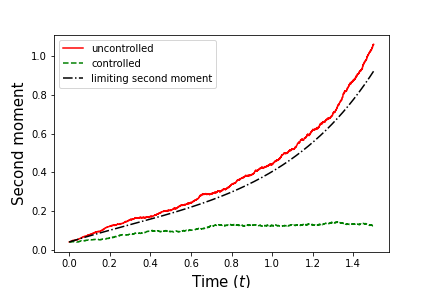
Refer to caption
(a)
Refer to caption
(b)
Figure 1. Left: An average of 5 realizations of the sum (54) for the uncontrolled (red) and controlled (green) particles respectively against the variance of the limiting McKean-Vlasov equation from (55) (black) for T∈[0,1.5]T\in[0,1.5], y=.2y=.2, and N=50N=50. Right: the log-scaled exact relative error ρ⁡(δN)\rho(\delta_{N}) as NN varies in the setting of Table 1, with M=1M=1 fixed in (16) (black) against the exact asymptotic rate ≈e.051​N\approx e^{.051N} (red).

4.2. Examples with Nonsmooth GG

Here we provide two examples where GG is not differentiable in the Lions sense (see Definition A.1). The first example is constructed via a perturbation of the linear-quadratic regime which reduces the smoothness of GG in a “global” way, whereas the second reduces the smoothness of GG in a “local” way. In both examples, despite the lack of regularity we observe that the relative error of the importance sampling scheme is much smaller than that of the standard Monte Carlo method for all NN. In Example 4.2, the relative error grows sublinearly, and in Example 4.1, the importance sampling relative error even appears to be vanishing, exhibiting that the assumptions in Theorems 2.4 and 2.5 are sufficient but not necessary. Thanks to the simple nature of the target function GG, we are able to provide an interpretation of the role of the controls in each example — see Remark 4.3.

Example 4.1.

In our second example, we consider

(58) G⁡(μ)=|∫ℝz​μ​(𝑑z)|,\displaystyle G(\mu)=\biggl|\int_{\mathbb{R}}z\mu(dz)\biggr|,

with drift and diffusion conforming to the linear-quadratic regime (44) with d=m=1d=m=1.

Note that while GG is continuous, it is not Lions differentiable at measures μ\mu such that ∫ℝz​μ​(𝑑z)=0\int_{\mathbb{R}}z\mu(dz)=0, so we are not able to obtain an explicit solution to the HJB equation (23) as in Section 3. However, for μ∈𝒫2​(ℝ)\mu\in\mathcal{P}_{2}(\mathbb{R}) with nonzero mean, it is plain to see that ∂μG⁡(μ)​[z]=sign​(∫ℝx​μ​(𝑑x))\partial_{\mu}G(\mu)[z]=\text{sign}\biggl(\int_{\mathbb{R}}x\mu(dx)\biggr) for all z∈ℝz\in\mathbb{R}, so ∂z∂μG⁡(μ)≡0\partial_{z}\partial_{\mu}G(\mu)\equiv 0 and ∂μ2G⁡(μ)≡0\partial^{2}_{\mu}G(\mu)\equiv 0. Using this ansatz, taking b0=0b_{0}=0, and performing a similar computation to [65] Section 4, we obtain the formal (weak) viscosity solution to (23) in this setting:

Ψ⁡(t,μ)=e(B+B¯)​[T−t]​|∫ℝz​μ​(𝑑z)|+σ24​(B+B¯)​[1−e2​(B+B¯)​(T−t)]\displaystyle\Psi(t,\mu)=e^{(B+\bar{B})[T-t]}\biggl|\int_{\mathbb{R}}z\mu(dz)\biggr|+\frac{\sigma^{2}}{4(B+\bar{B})}[1-e^{2(B+\bar{B})(T-t)}]

so that we expect the control from (33) in Theorem 2.4 to be of the form

v⁡(t,x1,…,xN)\displaystyle v(t,x_{1},...,x_{N}) =−σ∂μΨ(t,μxN)[xi]\displaystyle=-\sigma\partial_{\mu}\Psi(t,\mu^{N}_{x})[x_{i}]
=−σ​e(B+B¯)​(T−t)​sign​(1N​∑j=1Nxj).\displaystyle=-\sigma e^{(B+\bar{B})(T-t)}\text{sign}\biggl(\frac{1}{N}\sum_{j=1}^{N}x_{j}\biggr).

Indeed, via the equivalence with the small-noise regime as discussed in Remark 3.2, such a choice of control can be seen to solve the minimization problem (9) with F⁡(μ)=G⁡(μT)F(\mu)=G(\mu_{T}).

In Table 2, we provide for various NN the estimated expectation and empirical relative error for our importance sampling scheme compared with standard Monte Carlo, selecting B=−1B=-1, B¯=2,\bar{B}=2, s=0s=0, and yi=.4y_{i}=.4 for all i∈ℕi\in\mathbb{N}. As we see, the relative error for the importance sampling scheme seems to be vanishing as NN increases, whereas the standard Monte Carlo relative error increases exponentially.

IS Scheme Standard Monte Carlo
NN δ^N\hat{\delta}_{N} ρ~​(δ^N)\tilde{\rho}(\hat{\delta}_{N}) δN\delta_{N} ρ~​(δN)\tilde{\rho}(\delta_{N})
5 2.6644⋅10−22.6644\cdot 10^{-2} 3.7070⋅10−13.7070\cdot 10^{-1} 2.6653⋅10−22.6653\cdot 10^{-2} 2.99302.9930
10 9.0804⋅10−49.0804\cdot 10^{-4} 3.1427⋅10−13.1427\cdot 10^{-1} 9.2009⋅10−49.2009\cdot 10^{-4} 12.803212.8032
15 3.0269⋅10−53.0269\cdot 10^{-5} 2.6350⋅10−12.6350\cdot 10^{-1} 3.0645⋅10−53.0645\cdot 10^{-5} 53.941053.9410
20 9.9533⋅10−79.9533\cdot 10^{-7} 2.2227⋅10−12.2227\cdot 10^{-1} 1.0625⋅10−61.0625\cdot 10^{-6} 337.0401337.0401
25 3.2471⋅10−83.2471\cdot 10^{-8} 1.8900⋅10−11.8900\cdot 10^{-1} 3.5791⋅10−83.5791\cdot 10^{-8} 561.9164561.9164
30 1.0537⋅10−91.0537\cdot 10^{-9} 1.6154⋅10−11.6154\cdot 10^{-1} 1.2253⋅10−91.2253\cdot 10^{-9} 1016.16561016.1656
Table 2. Comparison of the standard Monte Carlo estimator δN\delta_{N} with the importance sampling estimator δ^N\hat{\delta}_{N} (14) and their corresponding relative errors ρ~​(δN)\tilde{\rho}(\delta_{N}) (57) and ρ~​(δ^N)\tilde{\rho}(\hat{\delta}_{N}) (56) with GG as in (58) and particles obeying (53) with initial condition y=.4y=.4 (Example 4.1).
Example 4.2.

.

IS Scheme Standard Monte Carlo
NN δ^N\hat{\delta}_{N} ρ~​(δ^N)\tilde{\rho}(\hat{\delta}_{N}) δN\delta_{N} ρ~​(δN)\tilde{\rho}(\delta_{N})
5 2.1355⋅10−22.1355\cdot 10^{-2} 4.7870⋅10−14.7870\cdot 10^{-1} 2.1382⋅10−22.1382\cdot 10^{-2} 2.32632.3263
10 5.6703⋅10−45.6703\cdot 10^{-4} 6.0605⋅10−16.0605\cdot 10^{-1} 5.6806⋅10−45.6806\cdot 10^{-4} 6.63746.6374
15 1.5087⋅10−51.5087\cdot 10^{-5} 7.2452⋅10−17.2452\cdot 10^{-1} 1.5040⋅10−51.5040\cdot 10^{-5} 17.333717.3337
20 4.0157⋅10−74.0157\cdot 10^{-7} 8.3416⋅10−18.3416\cdot 10^{-1} 4.1260⋅10−74.1260\cdot 10^{-7} 51.105851.1058
25 1.0687⋅10−81.0687\cdot 10^{-8} 9.4327⋅10−19.4327\cdot 10^{-1} 1.0296⋅10−81.0296\cdot 10^{-8} 97.882097.8820
30 2.8470⋅10−102.8470\cdot 10^{-10} 1.05241.0524 2.8800⋅10−102.8800\cdot 10^{-10} 280.5945280.5945
Table 3. Comparison of the standard Monte Carlo estimator δN\delta_{N} with the importance sampling estimator δ^N\hat{\delta}_{N} (14) and their corresponding relative errors ρ~​(δN)\tilde{\rho}(\delta_{N}) (57) and ρ~​(δ^N)\tilde{\rho}(\hat{\delta}_{N}) (56) with GG as in (59) and particles obeying (53) with initial condition y=.4y=.4 (Example 4.2).

Finally, we consider the same regime as Example 4.1, but now taking GG in the target expectation (3) to be:

(59) G⁡(μ)=∫ℝ|z|​μ​(𝑑z).\displaystyle G(\mu)=\int_{\mathbb{R}}|z|\mu(dz).

Once again GG is not everywhere Lions differentiable, in this case at measures such that the singleton {0}∈ℝ\{0\}\in\mathbb{R} has positive measure. Indeed, for μ∈𝒫2​(ℝ)\mu\in\mathcal{P}_{2}(\mathbb{R}) such that μ⁡({0})=0\mu(\{0\})=0, it is clear to see that ∂μG⁡(μ)​[z]=sign​(z)\partial_{\mu}G(\mu)[z]=\text{sign}(z), so ∂μ2G⁡(μ)=0\partial^{2}_{\mu}G(\mu)=0 and for z≠0z\neq 0, ∂z∂μG⁡(μ)​[z]=0\partial_{z}\partial_{\mu}G(\mu)[z]=0 (this follows via a similar computation to [15] Example 1 in Section 5.2.2).

Again we follow the methods of [65], taking b0=0b_{0}=0, and obtain the formal (weak) viscosity solution to (23):

Ψ⁡(t,μ)\displaystyle\Psi(t,\mu) =eB⁡(T−t)​∫ℝ|z|​μ​(𝑑z)+[e(B+B¯)​(T−t)−eB⁡(T−t)]​∫ℝz​μ​(𝑑z)​∫ℝsign​(z)​μ​(𝑑z)\displaystyle=e^{B(T-t)}\int_{\mathbb{R}}|z|\mu(dz)+[e^{(B+\bar{B})(T-t)}-e^{B(T-t)}]\int_{\mathbb{R}}z\mu(dz)\int_{\mathbb{R}}\text{sign}(z)\mu(dz)
+σ24​B​(B+B¯)​[e2​B​(T−t)​(B+B¯)−B​e2​(B+B¯)​(T−t)−B¯]​[∫ℝsign​(z)​μ​(𝑑z)]2+σ24​B​[1−e2​B​(T−t)].\displaystyle+\frac{\sigma^{2}}{4B(B+\bar{B})}[e^{2B(T-t)}(B+\bar{B})-Be^{2(B+\bar{B})(T-t)}-\bar{B}]\biggl[\int_{\mathbb{R}}\text{sign}(z)\mu(dz)\biggr]^{2}+\frac{\sigma^{2}}{4B}[1-e^{2B(T-t)}].

Using that for μ∈𝒫2​(ℝ)\mu\in\mathcal{P}_{2}(\mathbb{R}) with μ⁡({0})=0\mu(\{0\})=0, μ↦∫ℝsign​(z)​μ​(𝑑z)\mu\mapsto\int_{\mathbb{R}}\text{sign}(z)\mu(dz) is Lions differentiable with derivative 00, we expect the control from (33) in Theorem 2.4 to be of the form

v⁡(t,x1,…,xN)\displaystyle v(t,x_{1},...,x_{N}) =−σ∂μΨ(t,μxN)[xi]\displaystyle=-\sigma\partial_{\mu}\Psi(t,\mu^{N}_{x})[x_{i}]
=−σ⁡[eB⁡(T−t)​sign​(xi)+(e(B+B¯)​(T−t)−eB⁡(T−t))​1N​∑j=1Nsign​(xj)].\displaystyle=-\sigma\biggl[e^{B(T-t)}\text{sign}(x_{i})+\biggl(e^{(B+\bar{B})(T-t)}-e^{B(T-t)}\biggr)\frac{1}{N}\sum_{j=1}^{N}\text{sign}(x_{j})\biggr].

In Table 3, we provide for various NN the estimated expectation and empirical relative error for our importance sampling scheme compared with standard Monte Carlo, selecting B=−1B=-1, B¯=2\bar{B}=2, s=0s=0, and yi=.4y_{i}=.4 for all i∈ℕi\in\mathbb{N}. As we see, the importance sampling scheme has relative error which increases sublinearly as NN becomes large, in contrast to the standard Monte Carlo relative error which increases exponentially.

Remark 4.3.

We can think about the controls from Examples 4.1 and 4.2 in terms of the role they play in sampling the “rare event” of GG being close to 00 for the particle system in each case. When the absolute value appears outside the empirical mean, as in Example 4.1, we only need to be concerned with controlling the magnitude of the empirical mean, a characteristic of the particle ensemble. This is reflected in the controls, which are identical for every particle and force them in the opposite direction of the sign of the empirical mean. Meanwhile, in the situation of Example (4.2), to make GG close to zero we need the position of each individual particle to be near 00. Thus, the control uses information about the position of each particle relative to the origin. However, information about the ensemble of particles also still must appear because of the global interaction in the particles’ dynamics, which we see in the form of the difference in the proportions of the particles which are positive and negative at a given time.

We note that a similar combination of global information on the ensemble of particles and local information about the ii’th particle is also used for controls in the standard linear-quadratic regime of Section 3. See in particular the control used in our simple numerical example in Subsection 4.1. Numerical experiments confirm that the role of both the global and local information captured in the control is necessary for variance reduction in such cases. For example, using the simplified control v~​(t,x1,…,xN)=−σ​eB⁡(T−t)​sign​(xi)\tilde{v}(t,x_{1},...,x_{N})=-\sigma e^{B(T-t)}\text{sign}(x_{i}) in Example 4.2, we observed performance that was comparable or even worse than standard Monte Carlo.

It is also worth commenting on the choice of initial conditions in the examples of Subsection 4.2. We choose yi=.4y_{i}=.4 for all i∈ℕi\in\mathbb{N}, so that ν=δ.4\nu=\delta_{.4} is away from the region of discontinuity of ∂μΨ⁡(t,⋅)​[z]\partial_{\mu}\Psi(t,\cdot)[z]. We observed that if we took initial conditions such that ν\nu is closer to the region of discontinuity many more rogue trajectories appeared in the controlled dynamics and an extremely high sample size was needed before the importance sampling scheme could be seen to perform better than standard Monte Carlo. This is once again similar to the case of small-noise diffusions—see Table 3.1 compared to Table 3.2 in [76] and the discussion on pp. 1786-1787 therein.

We end this section by remarking on the interesting problem of verifying that the formal viscosity solutions to the HJB equation (23) constructed in Examples 4.1 and 4.2 are indeed viscosity solutions in the sense of [62]. To our knowledge, there are no existing examples in the current literature of explicit viscosity solutions which are not also classical solutions to an HJB equation on Wasserstein space.

5. Proof of the Main Results

We begin with a lemma which allows us to express the numerator of R⁡(δ^N)R(\hat{\delta}_{N}) (see (17)) in an alternative way:

Lemma 5.1.

Let Assumption 1.1 (A3) and Assumption 2.3 (B1) hold. Then, for any s∈[0,T],y1,…,yN∈ℝds\in[0,T],y_{1},...,y_{N}\in\mathbb{R}^{d}, and for μ^\hat{\mu} as in (15), Zi,N,s,yZ^{i,N,s,y} as in (13), and viN:[s,T]×ℝd​N→ℝm,i=1,…,Nv_{i}^{N}\mathrel{\mathop{\ordinarycolon}}[s,T]\times\mathbb{R}^{dN}\rightarrow\mathbb{R}^{m},i=1,...,N bounded:

𝔼⁡[exp⁡(−2​N​G​(μ^TN,s,y))​∏i=1N(Zi,N,s,y)2]=𝔼⁡[exp⁡(−2​N​G​(μ~TN,s,y))​exp⁡(∫sT∑i=1N|viN​(t,X~t1,N,s,y,…,X~tN,N)|2​𝑑t)],\displaystyle\mathbb{E}\biggl[\exp\left(-2NG(\hat{\mu}^{N,s,y}_{T})\right)\prod_{i=1}^{N}(Z^{i,N,s,y})^{2}\biggr]=\mathbb{E}\biggl[\exp\left(-2NG(\tilde{\mu}^{N,s,y}_{T})\right)\exp\biggl(\int_{s}^{T}\sum_{i=1}^{N}|v^{N}_{i}(t,\tilde{X}^{1,N,s,y}_{t},...,\tilde{X}^{N,N}_{t})|^{2}dt\biggr)\biggr],

where μ~tN,s,y=1N​∑i=1NδX~ti,N,s,y\tilde{\mu}^{N,s,y}_{t}=\frac{1}{N}\sum_{i=1}^{N}\delta_{\tilde{X}^{i,N,s,y}_{t}} and X~i,N,s,y\tilde{X}^{i,N,s,y} satisfy:

d​X~ti,N,s,y\displaystyle d\tilde{X}^{i,N,s,y}_{t} =[b⁡(X~ti,N,s,y,μ~tN,s,y)−σ⁡(X~ti,N,s,y,μ~tN,s,y)​viN​(t,X~t1,N,s,y,…,X~tN,N,s,y)]​d​t+σ⁡(X~ti,N,s,y,μ~tN,s,y)​d​W~ti,\displaystyle=[b(\tilde{X}^{i,N,s,y}_{t},\tilde{\mu}^{N,s,y}_{t})-\sigma(\tilde{X}^{i,N,s,y}_{t},\tilde{\mu}^{N,s,y}_{t})v^{N}_{i}(t,\tilde{X}^{1,N,s,y}_{t},...,\tilde{X}^{N,N,s,y}_{t})]dt+\sigma(\tilde{X}^{i,N,s,y}_{t},\tilde{\mu}^{N,s,y}_{t})d\tilde{W}^{i}_{t},
X~si,N,s,y\displaystyle\tilde{X}^{i,N,s,y}_{s} =yi,\displaystyle=y_{i},

and W~i\tilde{W}^{i} are IID standard mm-dimensional Brownian motions initialized at W~si=0\tilde{W}^{i}_{s}=0.

Proof.

This follows by a simple application of the Girsanov theorem, which is valid due to the boundedness of the viNv^{N}_{i}’s and GG. We have:

𝔼⁡[exp⁡(−2​N​G​(μ^TN,s,y))​∏i=1N(Zi,N,s,y)2]\displaystyle\mathbb{E}\biggl[\exp\left(-2NG(\hat{\mu}^{N,s,y}_{T})\right)\prod_{i=1}^{N}(Z^{i,N,s,y})^{2}\biggr]
=𝔼[exp(−2NG(μ^TN,s,y))exp(−2∑i=1N∫sTviN(t,X^t1,N,s,y,…,X^tN,N,s,y)⋅dW^ti\displaystyle=\mathbb{E}\biggl[\exp\left(-2NG(\hat{\mu}^{N,s,y}_{T})\right)\exp\biggl(-2\sum_{i=1}^{N}\int_{s}^{T}v^{N}_{i}(t,\hat{X}^{1,N,s,y}_{t},...,\hat{X}^{N,N,s,y}_{t})\cdot d\hat{W}^{i}_{t}
−∫sT∑i=1N|viN(t,X^t1,N,s,y,…,X^tN,N,s,y)|2dt)]\displaystyle-\int_{s}^{T}\sum_{i=1}^{N}|v^{N}_{i}(t,\hat{X}^{1,N,s,y}_{t},...,\hat{X}^{N,N,s,y}_{t})|^{2}dt\biggr)\biggr]
=𝔼[exp(−2NG(μ^TN,s,y))exp(−2∑i=1N∫sTviN(t,X^t1,N,s,y,…,X^tN,N,s,y)⋅dW^ti\displaystyle=\mathbb{E}\biggl[\exp\left(-2NG(\hat{\mu}^{N,s,y}_{T})\right)\exp\biggl(-2\sum_{i=1}^{N}\int_{s}^{T}v^{N}_{i}(t,\hat{X}^{1,N,s,y}_{t},...,\hat{X}^{N,N,s,y}_{t})\cdot d\hat{W}^{i}_{t}
−12∫sT∑i=1N|2viN(t,X^t1,N,s,y,…,X^tN,N,s,y)|2dt)exp(∫sT∑i=1N|viN(t,X^t1,N,s,y,…,X^tN,N,s,y)|2dt)]\displaystyle-\frac{1}{2}\int_{s}^{T}\sum_{i=1}^{N}|2v^{N}_{i}(t,\hat{X}^{1,N,s,y}_{t},...,\hat{X}^{N,N,s,y}_{t})|^{2}dt\biggr)\exp\biggl(\int_{s}^{T}\sum_{i=1}^{N}|v^{N}_{i}(t,\hat{X}^{1,N,s,y}_{t},...,\hat{X}^{N,N,s,y}_{t})|^{2}dt\biggr)\biggr]
=𝔼⁡[exp⁡(−2​N​G​(μ~TN,s,y))​exp⁡(∫sT∑i=1N|viN​(t,X~t1,N,s,y,…,X~tN,N)|2​𝑑t)].\displaystyle=\mathbb{E}\biggl[\exp\left(-2NG(\tilde{\mu}^{N,s,y}_{T})\right)\exp\biggl(\int_{s}^{T}\sum_{i=1}^{N}|v^{N}_{i}(t,\tilde{X}^{1,N,s,y}_{t},...,\tilde{X}^{N,N}_{t})|^{2}dt\biggr)\biggr].

∎

5.1. Proof of Theorem 2.4

Let Ψ\Psi be a classical subsolution to (23). We make the choice of control from (33) for (4) and (13) throughout this proof. Due to the assumed boundedness of these controls, we have via Lemma 5.1:

𝔼⁡[exp⁡(−2​N​G​(μ^TN,s,y))​∏i=1N(Zi,N,s,y)2]\displaystyle\mathbb{E}\biggl[\exp\left(-2NG(\hat{\mu}^{N,s,y}_{T})\right)\prod_{i=1}^{N}(Z^{i,N,s,y})^{2}\biggr]
=𝔼⁡[exp⁡(−2​N​G​(μ~TN,s,y))​exp⁡(N​∫sT∫ℝd|σ⊤​(x,μ~tN,s,y)​∂μΨ⁡(t,μ~tN)​[x]|2​μ~tN,s,y​(𝑑x)​𝑑t)],\displaystyle=\mathbb{E}\biggl[\exp\left(-2NG(\tilde{\mu}^{N,s,y}_{T})\right)\exp\biggl(N\int_{s}^{T}\int_{\mathbb{R}^{d}}|\sigma^{\top}(x,\tilde{\mu}^{N,s,y}_{t})\partial_{\mu}\Psi(t,\tilde{\mu}^{N}_{t})[x]|^{2}\tilde{\mu}^{N,s,y}_{t}(dx)dt\biggr)\biggr],

where μ~tN,s,y=1N​∑i=1NδX~ti,N,s,y\tilde{\mu}^{N,s,y}_{t}=\frac{1}{N}\sum_{i=1}^{N}\delta_{\tilde{X}^{i,N,s,y}_{t}} and X~i,N,s,y\tilde{X}^{i,N,s,y} satisfy:

d​X~ti,N,s,y\displaystyle d\tilde{X}^{i,N,s,y}_{t} =[b⁡(X~ti,N,s,y,μ~tN,s,y)+σ​σ⊤​(X~ti,N,s,y,μ~tN,s,y)​∂μΨ⁡(t,μ~tN,s,y)​[X~ti,N,s,y]]​d​t\displaystyle=[b(\tilde{X}^{i,N,s,y}_{t},\tilde{\mu}^{N,s,y}_{t})+\sigma\sigma^{\top}(\tilde{X}^{i,N,s,y}_{t},\tilde{\mu}^{N,s,y}_{t})\partial_{\mu}\Psi(t,\tilde{\mu}^{N,s,y}_{t})[\tilde{X}^{i,N,s,y}_{t}]]dt
+σ⁡(X~ti,N,s,y,μ~tN,s,y)​d​W~ti,X~si,N,s,y=yi.\displaystyle+\sigma(\tilde{X}^{i,N,s,y}_{t},\tilde{\mu}^{N,s,y}_{t})d\tilde{W}^{i}_{t},\quad\tilde{X}^{i,N,s,y}_{s}=y_{i}.

Strong existence and uniqueness of the above system of SDEs of all NN follows from the assumed boundedness of σ\sigma and ∂μΨ\partial_{\mu}\Psi along with Assumption (A3) and an application of Girsanov theorem—see the discussion on p.81 of [5].

Applying Proposition (1.3) with F⁡(μ)=2​G​(μT)−∫sT∫ℝd|σ⊤​(z,μt)​∂μΨ⁡(t,μt)​[z]|2​μt​(𝑑z)​𝑑tF(\mu)=2G(\mu_{T})-\int_{s}^{T}\int_{\mathbb{R}^{d}}|\sigma^{\top}(z,\mu_{t})\partial_{\mu}\Psi(t,\mu_{t})[z]|^{2}\mu_{t}(dz)dt (FF is bounded by assumption and its continuity follows from, e.g., [18] Theorem A.3.18) and b~​(t,x,ν)=b⁡(x,ν)+σ​σ⊤​(x,ν)​∂μΨ⁡(t,ν)​[x]\tilde{b}(t,x,\nu)=b(x,\nu)+\sigma\sigma^{\top}(x,\nu)\partial_{\mu}\Psi(t,\nu)[x], we get

(60) −1Nlog𝔼[exp(−2NG(μ^N,s,yT))∏i=1N(Zi,N,s,y)2]=infuN∈𝒰N{𝔼[12​N∑i=1N∫sT|uNi(t)|2dt]+2𝔼[G(μ¯N,s,yT)]−𝔼[1N∑i=1N∫sT|σ⊤(X¯i,N,s,yt,μ¯N,s,y)∂μΨ(t,μ¯N,s,yt)[X¯i,N,s,yt]|2dt]},\begin{split}-\frac{1}{N}\log\mathbb{E}\biggl[\exp\left(-2NG(\hat{\mu}^{N,s,y}_{T})\right)\prod_{i=1}^{N}(Z^{i,N,s,y})^{2}\biggr]=\inf_{u^{N}\in\mathcal{U}^{N}}\left\{\mathbb{E}\left[\frac{1}{2N}\sum_{i=1}^{N}\int_{s}^{T}|u^{N}_{i}(t)|^{2}dt\right]+2\mathbb{E}\left[G(\bar{\mu}^{N,s,y}_{T})\right]\right.&\\ \left.-\mathbb{E}\left[\frac{1}{N}\sum_{i=1}^{N}\int_{s}^{T}|\sigma^{\top}(\bar{X}^{i,N,s,y}_{t},\bar{\mu}^{N,s,y})\partial_{\mu}\Psi(t,\bar{\mu}^{N,s,y}_{t})[\bar{X}^{i,N,s,y}_{t}]|^{2}dt\right]\right\}&,\end{split}

where μ¯tN,s,y=1N​∑i=1NδX¯ti,N,s,y\bar{\mu}^{N,s,y}_{t}=\frac{1}{N}\sum_{i=1}^{N}\delta_{\bar{X}^{i,N,s,y}_{t}} and

d​X¯ti,N,s,y\displaystyle d\bar{X}^{i,N,s,y}_{t} =[b⁡(X¯ti,N,s,y,μ¯tN,s,y)+σ​σ⊤​(X¯ti,N,s,y,μ¯tN,s,y)​∂μΨ⁡(t,μ¯tN,s,y)​[X¯ti,N,s,y]+σ⁡(X¯ti,N,s,y,μ¯tN,s,y)​uiN​(t)]​d​t\displaystyle=[b(\bar{X}^{i,N,s,y}_{t},\bar{\mu}^{N,s,y}_{t})+\sigma\sigma^{\top}(\bar{X}^{i,N,s,y}_{t},\bar{\mu}^{N,s,y}_{t})\partial_{\mu}\Psi(t,\bar{\mu}^{N,s,y}_{t})[\bar{X}^{i,N,s,y}_{t}]+\sigma(\bar{X}^{i,N,s,y}_{t},\bar{\mu}^{N,s,y}_{t})u^{N}_{i}(t)]dt
+σ⁡(X¯ti,N,s,y,μ¯tN,s,y)​d​W~ti,\displaystyle+\sigma(\bar{X}^{i,N,s,y}_{t},\bar{\mu}^{N,s,y}_{t})d\tilde{W}^{i}_{t},
X¯si,N,s,y\displaystyle\bar{X}^{i,N,s,y}_{s} =yi.\displaystyle=y_{i}.

Fix any uN∈𝒰Nu^{N}\in\mathcal{U}^{N} and let {X¯i,N,s,y}i=1N\{\bar{X}^{i,N,s,y}\}_{i=1}^{N} satisfy the above controlled equations with this choice of control.

Letting Ψ~​(t,x1,…,xN)=Ψ⁡(t,1N​∑i=1Nδxi)\tilde{\Psi}(t,x_{1},...,x_{N})=\Psi(t,\frac{1}{N}\sum_{i=1}^{N}\delta_{x_{i}}), where Ψ\Psi is our classical subsolution, we apply Itô’s formula to get

d​Ψ​(t,μ¯tN,s,y)\displaystyle d\Psi(t,\bar{\mu}^{N,s,y}_{t})
=[∂tΨ(t,μ¯tN,s,y)+∑i=1N{[b(X¯ti,N,s,y,μ¯tN,s,y)+σσ⊤(X¯ti,N,s,y,μ¯tN,s,y)∂μΨ(t,μ¯tN,s,y)[X¯ti,N,s,y]\displaystyle=\biggl[\partial_{t}\Psi(t,\bar{\mu}^{N,s,y}_{t})+\sum_{i=1}^{N}\biggl\{[b(\bar{X}^{i,N,s,y}_{t},\bar{\mu}^{N,s,y}_{t})+\sigma\sigma^{\top}(\bar{X}^{i,N,s,y}_{t},\bar{\mu}^{N,s,y}_{t})\partial_{\mu}\Psi(t,\bar{\mu}^{N,s,y}_{t})[\bar{X}^{i,N,s,y}_{t}]
+σ(X¯ti,N,s,y,μ¯tN,s,y)uiN(t)]⋅∂xiΨ~(t,X¯ti,N,s,y,…,X¯tN,N,s,y)\displaystyle+\sigma(\bar{X}^{i,N,s,y}_{t},\bar{\mu}^{N,s,y}_{t})u^{N}_{i}(t)]\cdot\partial_{x_{i}}\tilde{\Psi}(t,\bar{X}^{i,N,s,y}_{t},...,\bar{X}^{N,N,s,y}_{t})
+12σσ⊤(X¯ti,N,s,y,μ¯tN,s,y):∂xi2Ψ~(t,X¯ti,N,s,y,…,X¯tN,N,s,y)}]dt\displaystyle+\frac{1}{2}\sigma\sigma^{\top}(\bar{X}^{i,N,s,y}_{t},\bar{\mu}^{N,s,y}_{t})\mathrel{\mathop{\ordinarycolon}}\partial^{2}_{x_{i}}\tilde{\Psi}(t,\bar{X}^{i,N,s,y}_{t},...,\bar{X}^{N,N,s,y}_{t})\biggr\}\biggr]dt
+∑i=1N[∂xiΨ~]⊤(t,X¯ti,N,s,y,…,X¯tN,N,s,y)σ(X¯ti,N,s,y,μ¯tN,s,y)dW~ti\displaystyle+\sum_{i=1}^{N}[\partial_{x_{i}}\tilde{\Psi}]^{\top}(t,\bar{X}^{i,N,s,y}_{t},...,\bar{X}^{N,N,s,y}_{t})\sigma(\bar{X}^{i,N,s,y}_{t},\bar{\mu}^{N,s,y}_{t})d\tilde{W}^{i}_{t}
=[∂tΨ(t,μ¯tN,s,y)+1N∑i=1N{[b(X¯ti,N,s,y,μ¯tN,s,y)+σσ⊤(X¯ti,N,s,y,μ¯tN,s,y)∂μΨ(t,μ¯tN,s,y)[X¯ti,N,s,y]\displaystyle=\biggl[\partial_{t}\Psi(t,\bar{\mu}^{N,s,y}_{t})+\frac{1}{N}\sum_{i=1}^{N}\biggl\{[b(\bar{X}^{i,N,s,y}_{t},\bar{\mu}^{N,s,y}_{t})+\sigma\sigma^{\top}(\bar{X}^{i,N,s,y}_{t},\bar{\mu}^{N,s,y}_{t})\partial_{\mu}\Psi(t,\bar{\mu}^{N,s,y}_{t})[\bar{X}^{i,N,s,y}_{t}]
+σ(X¯ti,N,s,y,μ¯tN,s,y)uiN(t)]⋅∂μΨ(t,μ¯tN,s,y)[X¯ti,N,s,y]+12σσ⊤(X¯ti,N,s,y,μ¯tN,s,y):∂z∂μΨ(t,μ¯tN,s,y)[X¯ti,N,s,y]}]dt\displaystyle+\sigma(\bar{X}^{i,N,s,y}_{t},\bar{\mu}^{N,s,y}_{t})u^{N}_{i}(t)]\cdot\partial_{\mu}\Psi(t,\bar{\mu}^{N,s,y}_{t})[\bar{X}^{i,N,s,y}_{t}]+\frac{1}{2}\sigma\sigma^{\top}(\bar{X}^{i,N,s,y}_{t},\bar{\mu}^{N,s,y}_{t})\mathrel{\mathop{\ordinarycolon}}\partial_{z}\partial_{\mu}\Psi(t,\bar{\mu}^{N,s,y}_{t})[\bar{X}^{i,N,s,y}_{t}]\biggr\}\biggr]dt
+1N∑i=1N[∂μΨ]⊤(t,μ¯tN,s,y)[X¯ti,N,s,y]σ(X¯ti,N,s,y,μ¯tN,s,y)dW~ti\displaystyle+\frac{1}{N}\sum_{i=1}^{N}[\partial_{\mu}\Psi]^{\top}(t,\bar{\mu}^{N,s,y}_{t})[\bar{X}^{i,N,s,y}_{t}]\sigma(\bar{X}^{i,N,s,y}_{t},\bar{\mu}^{N,s,y}_{t})d\tilde{W}^{i}_{t}
+1N2∑i=1Nσσ⊤(X¯ti,N,s,y,μ¯tN,s,y):∂μ2Ψ(t,μ¯tN,s,y)[X¯ti,N,s,y,X¯ti,N,s,y]dt,\displaystyle+\frac{1}{N^{2}}\sum_{i=1}^{N}\sigma\sigma^{\top}(\bar{X}^{i,N,s,y}_{t},\bar{\mu}^{N,s,y}_{t})\mathrel{\mathop{\ordinarycolon}}\partial^{2}_{\mu}\Psi(t,\bar{\mu}^{N,s,y}_{t})[\bar{X}^{i,N,s,y}_{t},\bar{X}^{i,N,s,y}_{t}]dt,

where in the second step we applied Proposition A.3. Note here we have used the assumed regularity of Ψ\Psi from (i) in Definition 2.1.

Now using that Ψ\Psi satisfies (ii) in Definition 2.1, we have:

∂tΨ(t,μ¯tN,s,y)+1N∑i=1N{[b(X¯ti,N,s,y,μ¯tN,s,y)\displaystyle\partial_{t}\Psi(t,\bar{\mu}^{N,s,y}_{t})+\frac{1}{N}\sum_{i=1}^{N}\biggl\{[b(\bar{X}^{i,N,s,y}_{t},\bar{\mu}^{N,s,y}_{t})
+σσ⊤(X¯ti,N,s,y,μ¯tN,s,y)∂μΨ(t,μ¯tN,s,y)[X¯ti,N,s,y]]⋅∂μΨ(t,μ¯tN,s,y)[X¯ti,N,s,y]\displaystyle\hskip 142.26378pt+\sigma\sigma^{\top}(\bar{X}^{i,N,s,y}_{t},\bar{\mu}^{N,s,y}_{t})\partial_{\mu}\Psi(t,\bar{\mu}^{N,s,y}_{t})[\bar{X}^{i,N,s,y}_{t}]]\cdot\partial_{\mu}\Psi(t,\bar{\mu}^{N,s,y}_{t})[\bar{X}^{i,N,s,y}_{t}]
+12σσ⊤(X¯ti,N,s,y,μ¯tN,s,y):∂z∂μΨ(t,μ¯tN,s,y)[X¯ti,N,s,y]}\displaystyle+\frac{1}{2}\sigma\sigma^{\top}(\bar{X}^{i,N,s,y}_{t},\bar{\mu}^{N,s,y}_{t})\mathrel{\mathop{\ordinarycolon}}\partial_{z}\partial_{\mu}\Psi(t,\bar{\mu}^{N,s,y}_{t})[\bar{X}^{i,N,s,y}_{t}]\biggr\}
≥32​1N​∑i=1N∂μΨ⁡(t,μ¯tN,s,y)​[X¯ti,N,s,y]⋅[σ​σ⊤​(X¯ti,N,s,y,μ¯tN,s,y)​∂μΨ⁡(t,μ¯tN,s,y)​[X¯ti,N,s,y]]\displaystyle\geq\frac{3}{2}\frac{1}{N}\sum_{i=1}^{N}\partial_{\mu}\Psi(t,\bar{\mu}^{N,s,y}_{t})[\bar{X}^{i,N,s,y}_{t}]\cdot[\sigma\sigma^{\top}(\bar{X}^{i,N,s,y}_{t},\bar{\mu}^{N,s,y}_{t})\partial_{\mu}\Psi(t,\bar{\mu}^{N,s,y}_{t})[\bar{X}^{i,N,s,y}_{t}]]
=32​1N​∑i=1N|σ⊤​(X¯ti,N,s,y,μ¯tN,s,y)​∂μΨ⁡(t,μ¯tN,s,y)​[X¯ti,N,s,y]|2.\displaystyle=\frac{3}{2}\frac{1}{N}\sum_{i=1}^{N}|\sigma^{\top}(\bar{X}^{i,N,s,y}_{t},\bar{\mu}^{N,s,y}_{t})\partial_{\mu}\Psi(t,\bar{\mu}^{N,s,y}_{t})[\bar{X}^{i,N,s,y}_{t}]|^{2}.

Combining the above two displays:

Ψ⁡(T,μ¯TN,s,y)\displaystyle\Psi(T,\bar{\mu}^{N,s,y}_{T}) ≥Ψ⁡(s,1N​∑i=1Nδyi)+1N​∑i=1N∫sTuiN​(t)⋅[σ⊤​(X¯ti,N,s,y,μ¯tN,s,y)​∂μΨ⁡(t,μ¯tN,s,y)​[X¯ti,N,s,y]]​𝑑t\displaystyle\geq\Psi\left(s,\frac{1}{N}\sum_{i=1}^{N}\delta_{y_{i}}\right)+\frac{1}{N}\sum_{i=1}^{N}\int_{s}^{T}u^{N}_{i}(t)\cdot[\sigma^{\top}(\bar{X}^{i,N,s,y}_{t},\bar{\mu}^{N,s,y}_{t})\partial_{\mu}\Psi(t,\bar{\mu}^{N,s,y}_{t})[\bar{X}^{i,N,s,y}_{t}]]dt
+1N∑i=1N∫sT[∂μΨ]⊤(t,μ¯tN,s,y)[X¯ti,N,s,y]σ(X¯ti,N,s,y,μ¯tN,s,y)dW~ti\displaystyle+\frac{1}{N}\sum_{i=1}^{N}\int_{s}^{T}[\partial_{\mu}\Psi]^{\top}(t,\bar{\mu}^{N,s,y}_{t})[\bar{X}^{i,N,s,y}_{t}]\sigma(\bar{X}^{i,N,s,y}_{t},\bar{\mu}^{N,s,y}_{t})d\tilde{W}^{i}_{t}
+1N2∑i=1N∫sTσσ⊤(X¯ti,N,s,y,μ¯tN,s,y):∂μ2Ψ(t,μ¯tN,s,y)[X¯ti,N,s,y,X¯ti,N,s,y]dt\displaystyle+\frac{1}{N^{2}}\sum_{i=1}^{N}\int_{s}^{T}\sigma\sigma^{\top}(\bar{X}^{i,N,s,y}_{t},\bar{\mu}^{N,s,y}_{t})\mathrel{\mathop{\ordinarycolon}}\partial^{2}_{\mu}\Psi(t,\bar{\mu}^{N,s,y}_{t})[\bar{X}^{i,N,s,y}_{t},\bar{X}^{i,N,s,y}_{t}]dt
+∫sT321N∑i=1N|σ⊤(X¯ti,N,s,y,μ¯tN,s,y)∂μΨ(t,μ¯tN,s,y)[X¯ti,N,s,y]|2dt\displaystyle+\int_{s}^{T}\frac{3}{2}\frac{1}{N}\sum_{i=1}^{N}|\sigma^{\top}(\bar{X}^{i,N,s,y}_{t},\bar{\mu}^{N,s,y}_{t})\partial_{\mu}\Psi(t,\bar{\mu}^{N,s,y}_{t})[\bar{X}^{i,N,s,y}_{t}]|^{2}dt
=Ψ⁡(s,1N​∑i=1Nδyi)+12​N​∑i=1N∫sT|uiN​(t)+σ⊤​(X¯ti,N,s,y,μ¯tN,s,y)​∂μΨ⁡(t,μ¯tN,s,y)​[X¯ti,N,s,y]|2​𝑑t\displaystyle=\Psi\left(s,\frac{1}{N}\sum_{i=1}^{N}\delta_{y_{i}}\right)+\frac{1}{2N}\sum_{i=1}^{N}\int_{s}^{T}|u^{N}_{i}(t)+\sigma^{\top}(\bar{X}^{i,N,s,y}_{t},\bar{\mu}^{N,s,y}_{t})\partial_{\mu}\Psi(t,\bar{\mu}^{N,s,y}_{t})[\bar{X}^{i,N,s,y}_{t}]|^{2}dt
+∫sT1N∑i=1N|σ⊤(X¯ti,N,s,y,μ¯tN,s,y)∂μΨ(t,μ¯tN,s,y)[X¯ti,N,s,y]|2dt\displaystyle+\int_{s}^{T}\frac{1}{N}\sum_{i=1}^{N}|\sigma^{\top}(\bar{X}^{i,N,s,y}_{t},\bar{\mu}^{N,s,y}_{t})\partial_{\mu}\Psi(t,\bar{\mu}^{N,s,y}_{t})[\bar{X}^{i,N,s,y}_{t}]|^{2}dt
−∫sT12​N∑i=1N|uiN(t)|2dt+1N∑i=1N∫sT[∂μΨ]⊤(t,μ¯tN,s,y)[X¯ti,N,s,y]σ(X¯ti,N,s,y,μ¯tN,s,y)dW~ti]\displaystyle-\int_{s}^{T}\frac{1}{2N}\sum_{i=1}^{N}|u^{N}_{i}(t)|^{2}dt+\frac{1}{N}\sum_{i=1}^{N}\int_{s}^{T}[\partial_{\mu}\Psi]^{\top}(t,\bar{\mu}^{N,s,y}_{t})[\bar{X}^{i,N,s,y}_{t}]\sigma(\bar{X}^{i,N,s,y}_{t},\bar{\mu}^{N,s,y}_{t})d\tilde{W}^{i}_{t}]
+1N2∑i=1N∫sTσσ⊤(X¯ti,N,s,y,μ¯tN,s,y):∂μΨ(t,μ¯tN,s,y)[X¯ti,N,s,y,X¯ti,N,s,y]dt.\displaystyle+\frac{1}{N^{2}}\sum_{i=1}^{N}\int_{s}^{T}\sigma\sigma^{\top}(\bar{X}^{i,N,s,y}_{t},\bar{\mu}^{N,s,y}_{t})\mathrel{\mathop{\ordinarycolon}}\partial_{\mu}\Psi(t,\bar{\mu}^{N,s,y}_{t})[\bar{X}^{i,N,s,y}_{t},\bar{X}^{i,N,s,y}_{t}]dt.

Then, for any choice of uN∈𝒰Nu^{N}\in\mathcal{U}^{N}:

𝔼⁡[12​N​∑i=1N∫sT|uiN​(t)|2​𝑑t]+2​𝔼​[G⁡(μ¯TN,s,y)]−𝔼⁡[1N​∑i=1N∫sT|σ⊤​(X¯ti,N,s,y,μ¯tN,s,y)​∂μΨ⁡(t,μ¯tN,s,y)​[X¯ti,N,s,y]|2​𝑑t]\displaystyle\mathbb{E}[\frac{1}{2N}\sum_{i=1}^{N}\int_{s}^{T}|u^{N}_{i}(t)|^{2}dt]+2\mathbb{E}\left[G(\bar{\mu}^{N,s,y}_{T})\right]-\mathbb{E}\left[\frac{1}{N}\sum_{i=1}^{N}\int_{s}^{T}|\sigma^{\top}(\bar{X}^{i,N,s,y}_{t},\bar{\mu}^{N,s,y}_{t})\partial_{\mu}\Psi(t,\bar{\mu}^{N,s,y}_{t})[\bar{X}^{i,N,s,y}_{t}]|^{2}dt\right]
≥𝔼⁡[G⁡(μ¯TN,s,y)]+𝔼⁡[Ψ⁡(T,μ¯TN,s,y)]+𝔼⁡[12​N​∑i=1N∫sT|uiN​(t)|2​𝑑t]\displaystyle\geq\mathbb{E}[G(\bar{\mu}^{N,s,y}_{T})]+\mathbb{E}[\Psi(T,\bar{\mu}^{N,s,y}_{T})]+\mathbb{E}\left[\frac{1}{2N}\sum_{i=1}^{N}\int_{s}^{T}|u^{N}_{i}(t)|^{2}dt\right]
−𝔼⁡[1N​∑i=1N∫sT|σ⊤​(X¯ti,N,s,y,μ¯tN,s,y)​∂μΨ⁡(t,μ¯tN,s,y)​[X¯ti,N,s,y]|2​𝑑t]\displaystyle-\mathbb{E}\left[\frac{1}{N}\sum_{i=1}^{N}\int_{s}^{T}|\sigma^{\top}(\bar{X}^{i,N,s,y}_{t},\bar{\mu}^{N,s,y}_{t})\partial_{\mu}\Psi(t,\bar{\mu}^{N,s,y}_{t})[\bar{X}^{i,N,s,y}_{t}]|^{2}dt\right]
≥𝔼⁡[G⁡(μ¯TN,s,y)]+Ψ⁡(s,1N​∑i=1Nδyi)+𝔼⁡[12​N​∑i=1N∫sT|uiN​(t)+σ⊤​(X¯ti,N,s,y,μ¯tN,s,y)​∂μΨ⁡(t,μ¯tN,s,y)​[X¯ti,N,s,y]|2​𝑑t]\displaystyle\geq\mathbb{E}[G(\bar{\mu}^{N,s,y}_{T})]+\Psi\left(s,\frac{1}{N}\sum_{i=1}^{N}\delta_{y_{i}}\right)+\mathbb{E}\left[\frac{1}{2N}\sum_{i=1}^{N}\int_{s}^{T}|u^{N}_{i}(t)+\sigma^{\top}(\bar{X}^{i,N,s,y}_{t},\bar{\mu}^{N,s,y}_{t})\partial_{\mu}\Psi(t,\bar{\mu}^{N,s,y}_{t})[\bar{X}^{i,N,s,y}_{t}]|^{2}dt\right]
+𝔼⁡[1N​∑i=1N∫sT[∂μΨ]⊤​(t,μ¯tN,s,y)​[X¯ti,N,s,y]​σ​(X¯ti,N,s,y,μ¯tN,s,y)​d​W~ti]\displaystyle+\mathbb{E}\left[\frac{1}{N}\sum_{i=1}^{N}\int_{s}^{T}[\partial_{\mu}\Psi]^{\top}(t,\bar{\mu}^{N,s,y}_{t})[\bar{X}^{i,N,s,y}_{t}]\sigma(\bar{X}^{i,N,s,y}_{t},\bar{\mu}^{N,s,y}_{t})d\tilde{W}^{i}_{t}\right]
+𝔼[1N2∑i=1N∫sTσσ⊤(X¯ti,N,s,y,μ¯tN,s,y):∂μ2Ψ(t,μ¯tN,s,y)[X¯ti,N,s,y,X¯ti,N,s,y]dt],\displaystyle+\mathbb{E}\left[\frac{1}{N^{2}}\sum_{i=1}^{N}\int_{s}^{T}\sigma\sigma^{\top}(\bar{X}^{i,N,s,y}_{t},\bar{\mu}^{N,s,y}_{t})\mathrel{\mathop{\ordinarycolon}}\partial^{2}_{\mu}\Psi(t,\bar{\mu}^{N,s,y}_{t})[\bar{X}^{i,N,s,y}_{t},\bar{X}^{i,N,s,y}_{t}]dt\right],

where in the first inequality we used (iii) from Definition 2.1.

uiN​(t)+σ⊤​(X¯ti,N,s,y,μ¯tN,s,y)​∂μΨ⁡(t,μ¯tN,s,y)​[X¯ti,N,s,y],i=1,…,Nu^{N}_{i}(t)+\sigma^{\top}(\bar{X}^{i,N,s,y}_{t},\bar{\mu}^{N,s,y}_{t})\partial_{\mu}\Psi(t,\bar{\mu}^{N,s,y}_{t})[\bar{X}^{i,N,s,y}_{t}],i=1,...,N is a valid choice of control in the prelimit representation (12) from Proposition 1.3 since σ\sigma, ∂μΨ\partial_{\mu}\Psi are bounded, and taking F⁡(μ)=G⁡(μT)F(\mu)=G(\mu_{T}), b~=b\tilde{b}=b therein (using G∈Cb​(𝒫⁡(ℝd))G\in C_{b}(\mathcal{P}(\mathbb{R}^{d})) and (A3)) we can continue:

𝔼⁡[12​N​∑i=1N∫sT|uiN​(t)|2​𝑑t]+2​𝔼​[G⁡(μ¯TN,s,y)]−𝔼⁡[1N​∑i=1N∫sT|σ⊤​(X¯ti,N,s,y,μ¯tN,s,y)​∂μΨ⁡(t,μ¯tN,s,y)​[X¯ti,N,s,y]|2​𝑑t]\displaystyle\mathbb{E}\left[\frac{1}{2N}\sum_{i=1}^{N}\int_{s}^{T}|u^{N}_{i}(t)|^{2}dt\right]+2\mathbb{E}\left[G(\bar{\mu}^{N,s,y}_{T})\right]-\mathbb{E}\left[\frac{1}{N}\sum_{i=1}^{N}\int_{s}^{T}|\sigma^{\top}(\bar{X}^{i,N,s,y}_{t},\bar{\mu}^{N,s,y}_{t})\partial_{\mu}\Psi(t,\bar{\mu}^{N,s,y}_{t})[\bar{X}^{i,N,s,y}_{t}]|^{2}dt\right]
≥Ψ⁡(s,1N​∑i=1Nδyi)+𝔼⁡[1N​∑i=1N∫sT[∂μΨ]⊤​(t,μ¯tN,s,y)​[X¯ti,N,s,y]​σ​(X¯ti,N,s,y,μ¯tN,s,y)​d​W~ti]\displaystyle\geq\Psi\left(s,\frac{1}{N}\sum_{i=1}^{N}\delta_{y_{i}}\right)+\mathbb{E}\left[\frac{1}{N}\sum_{i=1}^{N}\int_{s}^{T}[\partial_{\mu}\Psi]^{\top}(t,\bar{\mu}^{N,s,y}_{t})[\bar{X}^{i,N,s,y}_{t}]\sigma(\bar{X}^{i,N,s,y}_{t},\bar{\mu}^{N,s,y}_{t})d\tilde{W}^{i}_{t}\right]
+𝔼[1N2∑i=1N∫sTσσ⊤(X¯ti,N,s,y,μ¯tN,s,y):∂μ2Ψ(t,μ¯tN,s,y)[X¯ti,N,s,y,X¯ti,N,s,y]dt]\displaystyle+\mathbb{E}\left[\frac{1}{N^{2}}\sum_{i=1}^{N}\int_{s}^{T}\sigma\sigma^{\top}(\bar{X}^{i,N,s,y}_{t},\bar{\mu}^{N,s,y}_{t})\mathrel{\mathop{\ordinarycolon}}\partial^{2}_{\mu}\Psi(t,\bar{\mu}^{N,s,y}_{t})[\bar{X}^{i,N,s,y}_{t},\bar{X}^{i,N,s,y}_{t}]dt\right]
−1N​log⁡𝔼⁡[exp⁡(−N​G​(μTN,s,y))]\displaystyle-\frac{1}{N}\log\mathbb{E}\left[\exp\left(-NG(\mu_{T}^{N,s,y})\right)\right]
=Ψ(s,1N∑i=1Nδyi)+𝔼[1N2∑i=1N∫sTσσ⊤(X¯ti,N,s,y,μ¯tN,s,y):∂μ2Ψ(t,μ¯tN,s,y)[X¯ti,N,s,y,X¯ti,N,s,y]dt]\displaystyle=\Psi\left(s,\frac{1}{N}\sum_{i=1}^{N}\delta_{y_{i}}\right)+\mathbb{E}\left[\frac{1}{N^{2}}\sum_{i=1}^{N}\int_{s}^{T}\sigma\sigma^{\top}(\bar{X}^{i,N,s,y}_{t},\bar{\mu}^{N,s,y}_{t})\mathrel{\mathop{\ordinarycolon}}\partial^{2}_{\mu}\Psi(t,\bar{\mu}^{N,s,y}_{t})[\bar{X}^{i,N,s,y}_{t},\bar{X}^{i,N,s,y}_{t}]dt\right]
−1N​log⁡𝔼⁡[exp⁡(−N​G​(μTN,s,y))]\displaystyle-\frac{1}{N}\log\mathbb{E}\left[\exp\left(-NG(\mu_{T}^{N,s,y})\right)\right]

since the martingale term is bounded in square expectation for all NN.

Infimizing over uN∈𝒰Nu^{N}\in\mathcal{U}^{N} and using (60) we get:

lim infN→∞−1Nlog(𝔼[exp(−2NG(μ^TN,s,y))∏i=1N(Zi,N,s,y)2])\displaystyle\liminf_{N\rightarrow\infty}-\frac{1}{N}\log\biggl(\mathbb{E}\biggl[\exp\left(-2NG(\hat{\mu}^{N,s,y}_{T})\right)\prod_{i=1}^{N}(Z^{i,N,s,y})^{2}\biggr]\biggr)
≥lim infN→∞{Ψ(s,1N∑i=1Nδyi)\displaystyle\geq\liminf_{N\rightarrow\infty}\biggl\{\Psi\left(s,\frac{1}{N}\sum_{i=1}^{N}\delta_{y_{i}}\right)
+infuN∈𝒰N𝔼[1N2∑i=1N∫sTσσ⊤(X¯ti,N,s,y,μ¯tN,s,y):∂μ2Ψ(t,μ¯tN,s,y)[X¯ti,N,s,y,X¯ti,N,s,y]dt]\displaystyle+\inf_{u^{N}\in\mathcal{U}^{N}}\mathbb{E}\left[\frac{1}{N^{2}}\sum_{i=1}^{N}\int_{s}^{T}\sigma\sigma^{\top}(\bar{X}^{i,N,s,y}_{t},\bar{\mu}^{N,s,y}_{t})\mathrel{\mathop{\ordinarycolon}}\partial^{2}_{\mu}\Psi(t,\bar{\mu}^{N,s,y}_{t})[\bar{X}^{i,N,s,y}_{t},\bar{X}^{i,N,s,y}_{t}]dt\right]
−1Nlog𝔼[exp(−NG(μTN,s,y))]}\displaystyle-\frac{1}{N}\log\mathbb{E}\left[\exp(-NG(\mu_{T}^{N,s,y}))\right]\biggr\}
=Ψ⁡(s,ν)+γ1,\displaystyle=\Psi(s,\nu)+\gamma_{1},

where we used the assumed continuity of Ψ\Psi and the convergence of 1N​∑i=1Nδyi\frac{1}{N}\sum_{i=1}^{N}\delta_{y_{i}} to ν\nu, (18), and the fact that by boundedness of σ\sigma and (iv) in Definition 2.1, there is a constant CC independent on the choice of uN∈𝒰Nu^{N}\in\mathcal{U}^{N} (which may change from line to line) such that:

𝔼[1N2∑i=1N∫sTσσ⊤(X¯ti,N,s,y,μ¯tN,s,y):∂μ2Ψ(t,μ¯tN,s,y)[X¯ti,N,s,y,X¯ti,N,s,y]dt]\displaystyle\mathbb{E}\left[\frac{1}{N^{2}}\sum_{i=1}^{N}\int_{s}^{T}\sigma\sigma^{\top}(\bar{X}^{i,N,s,y}_{t},\bar{\mu}^{N,s,y}_{t})\mathrel{\mathop{\ordinarycolon}}\partial^{2}_{\mu}\Psi(t,\bar{\mu}^{N,s,y}_{t})[\bar{X}^{i,N,s,y}_{t},\bar{X}^{i,N,s,y}_{t}]dt\right]
≤C​𝔼​[1N2​∑i=1N∫sT|∂μ2Ψ⁡(t,μ¯tN,s,y)​[X¯ti,N,s,y,X¯ti,N,s,y]|​𝑑t]\displaystyle\leq C\mathbb{E}\left[\frac{1}{N^{2}}\sum_{i=1}^{N}\int_{s}^{T}|\partial^{2}_{\mu}\Psi(t,\bar{\mu}^{N,s,y}_{t})[\bar{X}^{i,N,s,y}_{t},\bar{X}^{i,N,s,y}_{t}]|dt\right]
=C​𝔼​[1N2​∑i=1N∑j=1N∫sT|∂μ2Ψ⁡(t,μ¯tN,s,y)​[X¯ti,N,s,y,X¯tj,N,s,y]|​𝟙i=j​𝑑t]\displaystyle=C\mathbb{E}\left[\frac{1}{N^{2}}\sum_{i=1}^{N}\sum_{j=1}^{N}\int_{s}^{T}|\partial^{2}_{\mu}\Psi(t,\bar{\mu}^{N,s,y}_{t})[\bar{X}^{i,N,s,y}_{t},\bar{X}^{j,N,s,y}_{t}]|\mathbbm{1}_{i=j}dt\right]
≤C​𝔼​[∫sT(1N2​∑i,j=1N|∂μ2Ψ⁡(t,μ¯tN,s,y)​[X¯ti,N,s,y,X¯tj,N,s,y]|2)1/2​(1N2​∑i,j=1N𝟙i=j)1/2​𝑑t]\displaystyle\leq C\mathbb{E}\left[\int_{s}^{T}\biggl({\frac{1}{N^{2}}}\sum_{i,j=1}^{N}|\partial^{2}_{\mu}\Psi(t,\bar{\mu}^{N,s,y}_{t})[\bar{X}^{i,N,s,y}_{t},\bar{X}^{j,N,s,y}_{t}]|^{2}\biggr)^{1/2}\biggl({\frac{1}{N^{2}}}\sum_{i,j=1}^{N}\mathbbm{1}_{i=j}\biggr)^{1/2}dt\right]
=C​𝔼​[1N1/2​∫sT(1N2​∑i,j=1N|∂μΨ⁡(t,μ¯tN,s,y)​[X¯ti,N,s,y,X¯tj,N,s,y]|2)1/2​𝑑t]\displaystyle=C\mathbb{E}\left[\frac{1}{N^{1/2}}\int_{s}^{T}\biggl(\frac{1}{N^{2}}\sum_{i,j=1}^{N}|\partial_{\mu}\Psi(t,\bar{\mu}^{N,s,y}_{t})[\bar{X}^{i,N,s,y}_{t},\bar{X}^{j,N,s,y}_{t}]|^{2}\biggr)^{1/2}dt\right]
=C​𝔼​[1N1/2​∫sT‖∂μ2Ψ⁡(t,μ¯tN,s,y)‖L2​(ℝd,μ¯tN,s,y)⊗L2​(ℝd,μ¯tN,s,y)​𝑑t]\displaystyle=C\mathbb{E}\left[\frac{1}{N^{1/2}}\int_{s}^{T}\mathinner{\!\left\lVert\partial^{2}_{\mu}\Psi(t,\bar{\mu}^{N,s,y}_{t})\right\rVert}_{L^{2}(\mathbb{R}^{d};\bar{\mu}^{N,s,y}_{t})\otimes L^{2}(\mathbb{R}^{d};\bar{\mu}^{N,s,y}_{t})}dt\right]
≤CN1/2​(T−s).\displaystyle\leq\frac{C}{N^{1/2}}(T-s).

Note that if we, instead of just the bound supt∈[0,T],μ∈𝒫2​(ℝd)‖∂μ2Ψ⁡(t,μ)​[⋅,⋅]‖L2​(ℝd,μ)⊗L2​(ℝd,μ)≤C\sup_{t\in[0,T],\mu\in\mathcal{P}_{2}(\mathbb{R}^{d})}\mathinner{\!\left\lVert\partial^{2}_{\mu}\Psi(t,\mu)[\cdot,\cdot]\right\rVert}_{L^{2}(\mathbb{R}^{d};\mu)\otimes L^{2}(\mathbb{R}^{d};\mu)}\leq C, have further that e.g. supt∈[0,T],μ∈𝒫2​(ℝd)∫ℝd|∂μ2Ψ⁡(t,μ)​[z,z]|2​μ​(𝑑z)≤C\sup_{t\in[0,T],\mu\in\mathcal{P}_{2}(\mathbb{R}^{d})}\int_{\mathbb{R}^{d}}|\partial^{2}_{\mu}\Psi(t,\mu)[z,z]|^{2}\mu(dz)\leq C, then this remainder is O⁡(1/N)O(1/N). Also note that the Laplace Principle of Theorem 1.2 is used here to establish the equality (18), which yields the appearance of γ1\gamma_{1} in the limit.

This gives that

limN→∞−1NlogR(δ^N)\displaystyle\lim_{N\rightarrow\infty}-\frac{1}{N}\log R(\hat{\delta}_{N})
=limN→∞{−1N​log⁡𝔼⁡[exp⁡(−2​N​G​(μ^N,s,y))​∏i=1N(Zi,N,s,y)2]+2N​log⁡𝔼⁡[exp⁡(−N​G​(μN,s,y))]}\displaystyle=\lim_{N\rightarrow\infty}\biggl\{-\frac{1}{N}\log\mathbb{E}\biggl[\exp(-2NG(\hat{\mu}^{N,s,y}))\prod_{i=1}^{N}(Z^{i,N,s,y})^{2}\biggr]+\frac{2}{N}\log\mathbb{E}\biggl[\exp(-NG(\mu^{N,s,y}))\biggr]\biggr\}
=limN→∞−1Nlog𝔼[exp(−2NG(μ^N,s,y))∏i=1N(Zi,N,s,y)2]−2γ1 (by (18))\displaystyle=\lim_{N\rightarrow\infty}-\frac{1}{N}\log\mathbb{E}\biggl[\exp(-2NG(\hat{\mu}^{N,s,y}))\prod_{i=1}^{N}(Z^{i,N,s,y})^{2}\biggr]-2\gamma_{1}\quad\text{ (by \eqref{eq:gammas})}
≥Ψ⁡(s,ν)−γ1.\displaystyle\geq\Psi(s,\nu)-\gamma_{1}.

We thus have that δ^N\hat{\delta}_{N} admits an expansion of the form (20) with γ^≤γ1−Ψ⁡(s,ν)\hat{\gamma}\leq\gamma_{1}-\Psi(s,\nu). Note that the case Ψ≡0\Psi\equiv 0 corresponds to the standard Monte Carlo estimator δN\delta_{N} in the above, from which we obtain γ=2​γ1−γ2≤γ1\gamma=2\gamma_{1}-\gamma_{2}\leq\gamma_{1} as expected – see (19) and the discussion thereafter. The rest of the claims stated in the theorem are now immediate. In particular, by Jensen’s inequality we know −1N​log⁡R⁡(δ^N)≤0-\frac{1}{N}\log R(\hat{\delta}_{N})\leq 0, so if Ψ⁡(s,ν)=γ1\Psi(s,\nu)=\gamma_{1} we have log-efficiency in the sense of Definition 1.4.

5.2. Proof of Theorem 2.5

First, we will establish a prelimit PDE expression for the numerator in the expression for R⁡(δ^N)R(\hat{\delta}_{N}) in (17) in a manner along the lines of the discussion in Section 2.1. Define

Ξ^N​(t,x1,…,xN)=𝔼⁡[exp⁡(−2​N​G​(μ^TN,t,x))​∏i=1N(Zi,N,t,x)2],x1,…,xN∈ℝd,t∈[0,T]\displaystyle\hat{\Xi}^{N}(t,x_{1},...,x_{N})=\mathbb{E}\biggl[\exp\left(-2NG(\hat{\mu}^{N,t,x}_{T})\right)\prod_{i=1}^{N}(Z^{i,N,t,x})^{2}\biggr],\quad x_{1},...,x_{N}\in\mathbb{R}^{d},t\in[0,T]{}

where Zi,N,t,x,i=1,…,NZ^{i,N,t,x},i=1,...,N and μ^N,t,x\hat{\mu}^{N,t,x} are as in (15) and (13) with the choice of controls from (33) in Theorem 2.4. Define v(t,μ,x)≔−σ⊤(x,μ)∂μϕ0(t,μ)[x]v(t,\mu,x)\coloneqq-\sigma^{\top}(x,\mu)\partial_{\mu}\phi_{0}(t,\mu)[x]. Then v⁡(t,μxN,xi)=viN​(t,x1,…,xN)v(t,\mu^{N}_{x},x_{i})=v_{i}^{N}(t,x_{1},...,x_{N}) for all NN, where viNv_{i}^{N} are from (33) with ϕ0\phi_{0} in the place of Ψ\Psi. Recall that in (33) we had only assumed Ψ\Psi be a classical subsolution of (23), whereas now we assume ϕ0\phi_{0} is a classical solution.

From Lemma 5.1 (using the assumed boundedness of σ\sigma and ∂μϕ0\partial_{\mu}\phi_{0}), we have:

(61) Ξ^N​(t,x1,…,xN)\displaystyle\hat{\Xi}^{N}(t,x_{1},...,x_{N}) =𝔼⁡[exp⁡(−2​N​G​(μ~TN,t,x))​exp⁡(N​∫tT∫ℝd|v⁡(τ,μ~τN,t,x,z)|2​μ~τN,t,x​(𝑑z)​𝑑τ)]\displaystyle=\mathbb{E}\biggl[\exp(-2NG(\tilde{\mu}^{N,t,x}_{T}))\exp\biggl(N\int_{t}^{T}\int_{\mathbb{R}^{d}}|v(\tau,\tilde{\mu}^{N,t,x}_{\tau},z)|^{2}\tilde{\mu}^{N,t,x}_{\tau}(dz)d\tau\biggr)\biggr]

where μ~τN,t,x=1N​∑i=1NδX~τi,N,t,x\tilde{\mu}^{N,t,x}_{\tau}=\frac{1}{N}\sum_{i=1}^{N}\delta_{\tilde{X}^{i,N,t,x}_{\tau}},

d​X~τi,N,t,x\displaystyle d\tilde{X}^{i,N,t,x}_{\tau} =[b⁡(X~τi,N,t,x,μ~τN,t,x)−σ⁡(X~τi,N,t,x,μ~τN,t,x)​v​(τ,μ~τN,t,x,X~τi,N,t,x)]​d​τ+σ⁡(X~τi,N,t,x,μ~τN,t,x)​d​W~τi,\displaystyle=[b(\tilde{X}^{i,N,t,x}_{\tau},\tilde{\mu}^{N,t,x}_{\tau})-\sigma(\tilde{X}^{i,N,t,x}_{\tau},\tilde{\mu}^{N,t,x}_{\tau})v(\tau,\tilde{\mu}^{N,t,x}_{\tau},\tilde{X}^{i,N,t,x}_{\tau})]d\tau+\sigma(\tilde{X}^{i,N,t,x}_{\tau},\tilde{\mu}^{N,t,x}_{\tau})d\tilde{W}^{i}_{\tau},
X~ti,N,t,x=xi.\displaystyle\tilde{X}^{i,N,t,x}_{t}=x_{i}.

Applying Feynman-Kac, we have Ξ^N\hat{\Xi}^{N} is the unique solution to:

(62) ∂tΞ^N​(t,x1,…,xN)+∑i=1N{[b(xi,μNx)−σ(xi,μNx)v(t,μNx,xi)]⋅∂xiΞ^N(t,x1,…,xN)+12σσ⊤(xi,μNx):∂2xiΞ^N(t,x1,…,xN)+|v(t,μNx,xi)|2Ξ^N(t,x1,…,xN)}=0,t∈[0,T),x1,…,xN∈ℝd,Ξ^N​(T,x1,…,xN)=exp⁡(−2​N​G​(μxN)),x1,…,xN∈ℝd.\begin{split}\partial_{t}\hat{\Xi}^{N}(t,x_{1},...,x_{N})&+\sum_{i=1}^{N}\biggl\{[b(x_{i},\mu^{N}_{x})-\sigma(x_{i},\mu^{N}_{x})v(t,\mu^{N}_{x},x_{i})]\cdot\partial_{x_{i}}\hat{\Xi}^{N}(t,x_{1},...,x_{N})\\ &+\frac{1}{2}\sigma\sigma^{\top}(x_{i},\mu^{N}_{x})\mathrel{\mathop{\ordinarycolon}}\partial^{2}_{x_{i}}\hat{\Xi}^{N}(t,x_{1},...,x_{N})+|v(t,\mu^{N}_{x},x_{i})|^{2}\hat{\Xi}^{N}(t,x_{1},...,x_{N})\biggr\}=0,\\ &\hskip 170.71652ptt\in[0,T),x_{1},...,x_{N}\in\mathbb{R}^{d},\\ \hat{\Xi}^{N}(T,x_{1},...,x_{N})&=\exp(-2NG(\mu^{N}_{x})),\qquad x_{1},...,x_{N}\in\mathbb{R}^{d}.\end{split}

This is where the linear growth condition on bb is used—see, e.g., Theorem 7.6 in [24].

Then Ξ~N​(t,x1,…,xN)≔−1N​log⁡Ξ^N​(t,x1,…,xN)\tilde{\Xi}^{N}(t,x_{1},...,x_{N})\coloneqq-\frac{1}{N}\log\hat{\Xi}^{N}(t,x_{1},...,x_{N}) satisfies

∂tΞ~N​(t,x1,…,xN)\displaystyle\partial_{t}\tilde{\Xi}^{N}(t,x_{1},...,x_{N}) +∑i=1N{[b(xi,μxN)−σ(xi,μxN)v(t,μxN,xi)]⋅∂xiΞ~N(t,x1,…,xN)\displaystyle+\sum_{i=1}^{N}\biggl\{[b(x_{i},\mu^{N}_{x})-\sigma(x_{i},\mu^{N}_{x})v(t,\mu^{N}_{x},x_{i})]\cdot\partial_{x_{i}}\tilde{\Xi}^{N}(t,x_{1},...,x_{N})
+12​σ​σ⊤​(xi,μxN):∂xi2Ξ~N​(t,x1,…,xN)−1N​|v⁡(t,μxN,xi)|2\displaystyle+\frac{1}{2}\sigma\sigma^{\top}(x_{i},\mu^{N}_{x})\mathrel{\mathop{\ordinarycolon}}\partial^{2}_{x_{i}}\tilde{\Xi}^{N}(t,x_{1},...,x_{N})-\frac{1}{N}|v(t,\mu^{N}_{x},x_{i})|^{2}
−N2|σ⊤(xi,μxN)∂xiΞ~N(t,x1,…,xN)|2}=0,t∈[0,T),x1,…,xN∈ℝd,\displaystyle-\frac{N}{2}|\sigma^{\top}(x_{i},\mu^{N}_{x})\partial_{x_{i}}\tilde{\Xi}^{N}(t,x_{1},...,x_{N})|^{2}\biggr\}=0,t\in[0,T),x_{1},...,x_{N}\in\mathbb{R}^{d},
Ξ~N​(T,x1,…,xN)\displaystyle\tilde{\Xi}^{N}(T,x_{1},...,x_{N}) =2​G​(μxN),x1,…,xN∈ℝd.\displaystyle=2G(\mu^{N}_{x}),\qquad x_{1},...,x_{N}\in\mathbb{R}^{d}.

We consider now the PDE (34) from Subsection 2.2. Note that this agrees with (32) if we set v≡0v\equiv 0, other than the fact that the terminal condition is 2​G2G rather than GG. Under the current regularity assumptions, we see via Proposition A.3 that for all NN, Ξ~N\tilde{\Xi}^{N} is the empirical projection of ΞN\Xi^{N} from (34). That is:

(63) ΞN​(t,μxN)=Ξ~N​(t,x1,…,xN)=−1N​log⁡𝔼⁡[exp⁡(−2​N​G​(μ^TN,t,x))​∏i=1N(Zi,N,t,x)2].\displaystyle\Xi^{N}(t,\mu^{N}_{x})=\tilde{\Xi}^{N}(t,x_{1},...,x_{N})=-\frac{1}{N}\log\mathbb{E}\biggl[\exp(-2NG(\hat{\mu}^{N,t,x}_{T}))\prod_{i=1}^{N}(Z^{i,N,t,x})^{2}\biggr].

We now observe how to uncover the log-efficiency established in Theorem 2.4 (though under stronger regularity assumptions) using the method of [72], and set up how higher order terms in such an expansion can be used to prove the results in Theorem 2.5.

Suppose, as in [72], that we have sufficient regularity to have the asymptotic expansions for (32) and (34) of the forms (36) and (37) for some kk.

Then by (61) and (25) (noting that indeed the representation (25) holds for the unique solution Φ^N\hat{\Phi}^{N} to (26), again by Theorem 7.6 in [24]), we have

R⁡(δ^N)\displaystyle R(\hat{\delta}_{N}) =Ξ^N​(s,y1,…,yN)[Φ^N​(s,y1,…,yN)]2\displaystyle=\frac{\hat{\Xi}^{N}(s,y_{1},...,y_{N})}{[\hat{\Phi}^{N}(s,y_{1},...,y_{N})]^{2}}
=exp⁡(N⁡[2​ϕ0​(s,μyN)−ξ0​(s,μyN)]+[2​ϕ1​(s,μyN)−ξ1​(s,μyN)]+[2​ϕ2​(s,μyN)−ξ2​(s,μyN)]/N+…CLOSE\displaystyle=\exp\biggl(N[2\phi_{0}(s,\mu^{N}_{y})-\xi_{0}(s,\mu^{N}_{y})]+[2\phi_{1}(s,\mu^{N}_{y})-\xi_{1}(s,\mu^{N}_{y})]+[2\phi_{2}(s,\mu^{N}_{y})-\xi_{2}(s,\mu^{N}_{y})]/N+...
+[2ϕk(s,μyN)−ξk(s,μyN)]/Nk−1+o(1/Nk−1)),\displaystyle\hskip 170.71652pt+[2\phi_{k}(s,\mu^{N}_{y})-\xi_{k}(s,\mu^{N}_{y})]/N^{k-1}+o(1/N^{k-1})\biggr),

where R⁡(δ^N)R(\hat{\delta}_{N}) is as in (17). Here we have used, by the same logic as to obtain (63),

ΦN​(t,μxN)=Φ~N​(t,x1,…,xN)=−1N​log⁡𝔼⁡[exp⁡(−N​G​(μTN,t,x))],\displaystyle\Phi^{N}(t,\mu^{N}_{x})=\tilde{\Phi}^{N}(t,x_{1},...,x_{N})=-\frac{1}{N}\log\mathbb{E}[\exp(-NG(\mu^{N,t,x}_{T}))],

where ΦN\Phi^{N} is as in (32) and Φ~N\tilde{\Phi}^{N} is as in (29).

We now see that 2​ϕ02\phi_{0} (recalling here that ϕ0\phi_{0} is the unique classical solution to (23)) and ξ0\xi_{0} from (35) satisfy the same equation. Indeed, inserting this ansatz into (35) and using v(t,μ,x)=−σ⊤(x,μ)∂μϕ0(t,μ)[x]v(t,\mu,x)=-\sigma^{\top}(x,\mu)\partial_{\mu}\phi_{0}(t,\mu)[x], we get

2​∂tϕ0​(t,μ)\displaystyle 2\partial_{t}\phi_{0}(t,\mu) +2∫ℝd[b(z,μ)+σσ⊤(z,μ)∂μϕ0(t,μ)[z]]⋅∂μϕ0(t,μ)[z]+12σσ⊤(z,μ):∂z∂μϕ0(t,μ)[z]μ(dz)\displaystyle+2\int_{\mathbb{R}^{d}}[b(z,\mu)+\sigma\sigma^{\top}(z,\mu)\partial_{\mu}\phi_{0}(t,\mu)[z]]\cdot\partial_{\mu}\phi_{0}(t,\mu)[z]+\frac{1}{2}\sigma\sigma^{\top}(z,\mu)\mathrel{\mathop{\ordinarycolon}}\partial_{z}\partial_{\mu}\phi_{0}(t,\mu)[z]\mu(dz)
−∫ℝd2|σ⊤(z,μ)∂μϕ0(t,μ)[z]|2+|σ⊤(z,μ)∂μϕ0(t,μ)[z]|2μ(dz)\displaystyle-\int_{\mathbb{R}^{d}}2|\sigma^{\top}(z,\mu)\partial_{\mu}\phi_{0}(t,\mu)[z]|^{2}+|\sigma^{\top}(z,\mu)\partial_{\mu}\phi_{0}(t,\mu)[z]|^{2}\mu(dz)
=2​∂tϕ0​(t,μ)+2​∫ℝdb⁡(z,μ)⋅∂μϕ0​(t,μ)​[z]+12​σ​σ⊤​(z,μ):∂z∂μϕ0​(t,μ)​[z]​μ​(𝑑z)\displaystyle=2\partial_{t}\phi_{0}(t,\mu)+2\int_{\mathbb{R}^{d}}b(z,\mu)\cdot\partial_{\mu}\phi_{0}(t,\mu)[z]+\frac{1}{2}\sigma\sigma^{\top}(z,\mu)\mathrel{\mathop{\ordinarycolon}}\partial_{z}\partial_{\mu}\phi_{0}(t,\mu)[z]\mu(dz)
−∫ℝd|σ⊤(z,μ)∂μϕ0(t,μ)[z]|2μ(dz)=0,t∈[0,T),μ∈𝒫2(ℝd),\displaystyle-\int_{\mathbb{R}^{d}}|\sigma^{\top}(z,\mu)\partial_{\mu}\phi_{0}(t,\mu)[z]|^{2}\mu(dz)=0,\qquad t\in[0,T),\mu\in\mathcal{P}_{2}(\mathbb{R}^{d}),
2​ϕ0​(T,μ)\displaystyle 2\phi_{0}(T,\mu) =2​G​(μ),μ∈𝒫2​(ℝd).\displaystyle=2G(\mu),\qquad\mu\in\mathcal{P}_{2}(\mathbb{R}^{d}).

which dividing by 22 gives the same equation as (23).

This shows that indeed 2​ϕ0​(t,μ)=ξ0​(t,μ)2\phi_{0}(t,\mu)=\xi_{0}(t,\mu) for all t∈[0,T],μ∈𝒫2​(ℝd)t\in[0,T],\mu\in\mathcal{P}_{2}(\mathbb{R}^{d}) via our uniqueness assumption.

Thus, since 2​ϕ0​(s,μyN)=ξ0​(s,μyN)2\phi_{0}(s,\mu^{N}_{y})=\xi_{0}(s,\mu^{N}_{y}) for all NN, we have −1N​log⁡R⁡(δ^N)→0-\frac{1}{N}\log R(\hat{\delta}_{N})\rightarrow 0 as N→∞N\rightarrow\infty.

Moreover, when k=1k=1, knowing 2​ϕ0​(s,μyN)=ξ0​(s,μyN)2\phi_{0}(s,\mu^{N}_{y})=\xi_{0}(s,\mu^{N}_{y}), we have for any MM

limN→∞ρ⁡(δ^N)=1M​limN→∞exp⁡(2​ϕ1​(s,μyN)−ξ1​(s,μyN)+o⁡(1))−1.\displaystyle\lim_{N\rightarrow\infty}\rho(\hat{\delta}_{N})=\frac{1}{\sqrt{M}}\sqrt{\lim_{N\rightarrow\infty}\exp(2\phi_{1}(s,\mu^{N}_{y})-\xi_{1}(s,\mu^{N}_{y})+o(1))-1}.

As we will show, under our current assumptions 2​ϕ1​(s,μyN)=ξ1​(s,μyN)2\phi_{1}(s,\mu^{N}_{y})=\xi_{1}(s,\mu^{N}_{y}) for all NN, so we get limN→∞ρ⁡(δ^N)=0\lim_{N\rightarrow\infty}\rho(\hat{\delta}_{N})=0, yielding vanishing relative error (Definition 1.5).

Lastly, knowing 2​ϕ0​(s,μyN)=ξ0​(s,μyN)2\phi_{0}(s,\mu^{N}_{y})=\xi_{0}(s,\mu^{N}_{y}) and 2​ϕ1​(s,μyN)=ξ1​(s,μyN)2\phi_{1}(s,\mu^{N}_{y})=\xi_{1}(s,\mu^{N}_{y}), letting k=2k=2 we have:

limN→∞T⁡(N)\displaystyle\lim_{N\rightarrow\infty}T(N) =limN→∞N⁡[exp⁡([2​ϕ2​(s,μyN)−ξ2​(s,μyN)]/N+o⁡(1/N))−1]\displaystyle=\lim_{N\rightarrow\infty}N[\exp([2\phi_{2}(s,\mu^{N}_{y})-\xi_{2}(s,\mu^{N}_{y})]/N+o(1/N))-1]
=limN→∞[2​ϕ2​(s,μyN)−ξ2​(s,μyN)]+o⁡(1)\displaystyle=\lim_{N\rightarrow\infty}[2\phi_{2}(s,\mu^{N}_{y})-\xi_{2}(s,\mu^{N}_{y})]+o(1)
=limN→∞[2​ϕ2​(s,μyN)−ξ2​(s,μyN)]\displaystyle=\lim_{N\rightarrow\infty}[2\phi_{2}(s,\mu^{N}_{y})-\xi_{2}(s,\mu^{N}_{y})]
=2​ϕ2​(s,ν)−ξ2​(s,ν)\displaystyle=2\phi_{2}(s,\nu)-\xi_{2}(s,\nu)

where T⁡(N)T(N) is as in (42) and here we have used the assumed continuity of ϕ2,ξ2\phi_{2},\xi_{2}. This will yield the limit (43).

We now insert the ansatz of the expansions (36) for ΦN​(t,μ)\Phi^{N}(t,\mu) and (37) for ΞN​(t,μ)\Xi^{N}(t,\mu) into their respective equations (32) and (34) and match 𝒪⁡(1/Nk)\mathcal{O}(1/N^{k}) to obtain formal recursive formulas for ξk\xi_{k} and ϕk\phi_{k} as in Theorem 3.3 in [72]. We arrive at the expressions (38) and (39) from Subsection 2.2.

Now recalling 2​ϕ0​(t,μ)=ξ0​(t,μ)2\phi_{0}(t,\mu)=\xi_{0}(t,\mu), we see that in (40) and (41) from Subsection 2.2, Yt,μ​=𝑑​Zt,μY^{t,\mu}\overset{d}{=}Z^{t,\mu} (using (A4)), and moreover we note that Zt,μZ^{t,\mu} is the solution to the (optimally) controlled limiting McKean-Vlasov equation initialized at time tt with distribution μ\mu from Theorem 1.2, that is Zt,μ​=𝑑​X^u,t,μZ^{t,\mu}\overset{d}{=}\hat{X}^{u,t,\mu} from (8) with
u(τ)=−σ(X^τu,t,ν,ℒ(X^τu,t,ν))∂μϕ0(τ,ℒ(X^τu,t,ν))[X^τu,t,ν],τ∈[t,T]u(\tau)=-\sigma(\hat{X}^{u,t,\nu}_{\tau},\mathcal{L}(\hat{X}^{u,t,\nu}_{\tau}))\partial_{\mu}\phi_{0}(\tau,\mathcal{L}(\hat{X}^{u,t,\nu}_{\tau}))[\hat{X}^{u,t,\nu}_{\tau}],{\tau\in[t,T]}.

Under the assumption that the expressions (40),(41) are valid with k=1k=1, we have:

ϕ1​(t,μ)\displaystyle\phi_{1}(t,\mu) =12𝔼[∫tTσσ⊤(Zτt,μ,ℒ(Zτt,μ)):∂μ2ϕ0(τ,ℒ(Zτt,μ))[Zτt,μ,Zτt,μ]dτ]\displaystyle=\frac{1}{2}\mathbb{E}\biggl[\int_{t}^{T}\sigma\sigma^{\top}(Z^{t,\mu}_{\tau},\mathcal{L}(Z^{t,\mu}_{\tau}))\mathrel{\mathop{\ordinarycolon}}\partial^{2}_{\mu}\phi_{0}(\tau,\mathcal{L}(Z^{t,\mu}_{\tau}))[Z^{t,\mu}_{\tau},Z^{t,\mu}_{\tau}]d\tau\biggr]

and

ξ1​(t,μ)\displaystyle\xi_{1}(t,\mu) =𝔼[∫tT12σσ⊤(Zτt,μ,ℒ(Zτt,μ)):∂μ2ξ0(τ,ℒ(Zτt,μ))[Zτt,μ,Zτt,μ]dτ]\displaystyle=\mathbb{E}\biggl[\int_{t}^{T}\frac{1}{2}\sigma\sigma^{\top}(Z^{t,\mu}_{\tau},\mathcal{L}(Z^{t,\mu}_{\tau}))\mathrel{\mathop{\ordinarycolon}}\partial^{2}_{\mu}\xi_{0}(\tau,\mathcal{L}(Z^{t,\mu}_{\tau}))[Z^{t,\mu}_{\tau},Z^{t,\mu}_{\tau}]d\tau\biggr]
=𝔼[∫tTσσ⊤(Zτt,μ,ℒ(Zτt,μ)):∂μ2ϕ0(τ,ℒ(Zτt,μ))[Zτt,μ,Zτt,μ]dτ],\displaystyle=\mathbb{E}\biggl[\int_{t}^{T}\sigma\sigma^{\top}(Z^{t,\mu}_{\tau},\mathcal{L}(Z^{t,\mu}_{\tau}))\mathrel{\mathop{\ordinarycolon}}\partial^{2}_{\mu}\phi_{0}(\tau,\mathcal{L}(Z^{t,\mu}_{\tau}))[Z^{t,\mu}_{\tau},Z^{t,\mu}_{\tau}]d\tau\biggr],

so indeed ξ1​(t,μ)=2​ϕ1​(t,μ)\xi_{1}(t,\mu)=2\phi_{1}(t,\mu) for all t∈[0,T]t\in[0,T] and μ∈𝒫2​(ℝd)\mu\in\mathcal{P}_{2}(\mathbb{R}^{d}). As discussed previously, this establishes that we indeed have vanishing relative error (Definition 1.5). Also, this is the expected expression to arrive at for these first-order correction terms—compare with equations (A.7) and (A.8) in [76], where the analogous expression is given in terms of the second derivative of their zero-viscosity (standard) HJB equation evaluated at the optimally controlled path for the limiting ODE in the small-noise regime.

Under the additional assumption that our representations (40),(41) for ϕk,ξk\phi_{k},\xi_{k} hold for the next order correction k=2k=2, we have:

ϕ2​(t,μ)\displaystyle\phi_{2}(t,\mu) =12𝔼[∫tTσσ⊤(Zτt,μ,ℒ(Zτt,μ)):∂μ2ϕ1(τ,ℒ(Zτt,μ))[Zτt,μ,Zτt,μ]\displaystyle=\frac{1}{2}\mathbb{E}\biggl[\int_{t}^{T}\sigma\sigma^{\top}(Z^{t,\mu}_{\tau},\mathcal{L}(Z^{t,\mu}_{\tau}))\mathrel{\mathop{\ordinarycolon}}\partial^{2}_{\mu}\phi_{1}(\tau,\mathcal{L}(Z^{t,\mu}_{\tau}))[Z^{t,\mu}_{\tau},Z^{t,\mu}_{\tau}]
−|σ⊤(Zτt,μ,ℒ(Zτt,μ))∂μϕ1(τ,ℒ(Zτt,μ))[Zτt,μ]|2dτ]\displaystyle\hskip 113.81102pt-|\sigma^{\top}(Z^{t,\mu}_{\tau},\mathcal{L}(Z^{t,\mu}_{\tau}))\partial_{\mu}\phi_{1}(\tau,\mathcal{L}(Z^{t,\mu}_{\tau}))[Z^{t,\mu}_{\tau}]|^{2}d\tau\biggr]

and

ξ2​(t,μ)\displaystyle\xi_{2}(t,\mu) =𝔼[∫tT12σσ⊤(Zτt,μ,ℒ(Zτt,μ)):∂μ2ξ1(τ,ℒ(Zτt,μ))[Zτt,μ,Zτt,μ]\displaystyle=\mathbb{E}\biggl[\int_{t}^{T}\frac{1}{2}\sigma\sigma^{\top}(Z^{t,\mu}_{\tau},\mathcal{L}(Z^{t,\mu}_{\tau}))\mathrel{\mathop{\ordinarycolon}}\partial^{2}_{\mu}\xi_{1}(\tau,\mathcal{L}(Z^{t,\mu}_{\tau}))[Z^{t,\mu}_{\tau},Z^{t,\mu}_{\tau}]
−12|σ⊤(Zτt,μ,ℒ(Zτt,μ))∂μξ1(τ,ℒ(Zτt,μ))[Zτt,μ]|2dτ]\displaystyle\hskip 113.81102pt-\frac{1}{2}|\sigma^{\top}(Z^{t,\mu}_{\tau},\mathcal{L}(Z^{t,\mu}_{\tau}))\partial_{\mu}\xi_{1}(\tau,\mathcal{L}(Z^{t,\mu}_{\tau}))[Z^{t,\mu}_{\tau}]|^{2}d\tau\biggr]
=𝔼[∫tTσσ⊤(Zτt,μ,ℒ(Zτt,μ)):∂μ2ϕ1(τ,ℒ(Zτt,μ))[Zτt,μ,Zτt,μ]dτ\displaystyle=\mathbb{E}\biggl[\int_{t}^{T}\sigma\sigma^{\top}(Z^{t,\mu}_{\tau},\mathcal{L}(Z^{t,\mu}_{\tau}))\mathrel{\mathop{\ordinarycolon}}\partial^{2}_{\mu}\phi_{1}(\tau,\mathcal{L}(Z^{t,\mu}_{\tau}))[Z^{t,\mu}_{\tau},Z^{t,\mu}_{\tau}]d\tau
−2|σ⊤(Zτt,μ,ℒ(Zτt,μ))∂μϕ1(τ,ℒ(Zτt,μ))[Zτt,μ]|2dτ],\displaystyle\hskip 113.81102pt-2|\sigma^{\top}(Z^{t,\mu}_{\tau},\mathcal{L}(Z^{t,\mu}_{\tau}))\partial_{\mu}\phi_{1}(\tau,\mathcal{L}(Z^{t,\mu}_{\tau}))[Z^{t,\mu}_{\tau}]|^{2}d\tau\biggr],

so

2​ϕ2​(t,μ)−ξ2​(t,μ)=𝔼⁡[∫tT|σ⊤​(Zτt,μ,ℒ⁡(Zτt,μ))​∂μϕ1​(τ,ℒ⁡(Zτt,μ))​[Zτt,μ]|2​𝑑τ].\displaystyle 2\phi_{2}(t,\mu)-\xi_{2}(t,\mu)=\mathbb{E}\biggl[\int_{t}^{T}|\sigma^{\top}(Z^{t,\mu}_{\tau},\mathcal{L}(Z^{t,\mu}_{\tau}))\partial_{\mu}\phi_{1}(\tau,\mathcal{L}(Z^{t,\mu}_{\tau}))[Z^{t,\mu}_{\tau}]|^{2}d\tau\biggr].

By our previous discussion and our identification of Zt,μZ^{t,\mu} as related to X^u,t,μ\hat{X}^{u,t,\mu}, we get

limN→∞T⁡(N)=𝔼⁡[∫sT|σ⊤​(X^tu,s,ν,ℒ⁡(X^tu,s,ν))​∂μϕ1​(t,ℒ⁡(X^tu,s,ν))​[X^tu,s,ν]|2​𝑑t]\displaystyle\lim_{N\rightarrow\infty}T(N)=\mathbb{E}\biggl[\int_{s}^{T}|\sigma^{\top}(\hat{X}^{u,s,\nu}_{t},\mathcal{L}(\hat{X}^{u,s,\nu}_{t}))\partial_{\mu}\phi_{1}(t,\mathcal{L}(\hat{X}^{u,s,\nu}_{t}))[\hat{X}^{u,s,\nu}_{t}]|^{2}dt\biggr]

where ϕ1\phi_{1} is as in (38) with k=1k=1 and u(t)=−σ⊤(X^tu,s,ν,ℒ(X^tu,s,ν))∂μϕ0(t,ℒ(X^tu,s,ν))[X^tu,s,ν],t∈[s,T]u(t)=-\sigma^{\top}(\hat{X}^{u,s,\nu}_{t},\mathcal{L}(\hat{X}^{u,s,\nu}_{t}))\partial_{\mu}\phi_{0}(t,\mathcal{L}(\hat{X}^{u,s,\nu}_{t}))[\hat{X}^{u,s,\nu}_{t}]{,t\in[s,T]}.

6. Conclusions and Future Work

We have derived an importance sampling scheme for exponential functionals of the empirical measure of weakly interacting diffusions. Using the connection between the large deviations rate function of [5] and mean-field optimal control, the asymptotic performance of the proposed scheme is characterized in terms of subsolutions of the Hamilton-Jacobi-Bellman equation on Wasserstein space. We provide both numerical and analytical evidence that sufficient smoothness of such a solution can yield relative error which vanishes as the number of particles becomes large. We also numerically explore the impact of lack of smoothness of the solution of the HJB equation on the performance of the proposed importance sampling scheme.

In future work, a major hurdle to overcome will be adapting the scheme to situations where subsolutions of the HJB equation cannot be constructed analytically. In the standard small noise setting, this is also a major issue, and when the dimension of the system becomes large advanced techniques such as the use of machine learning, optimization software, and neural networks to identify the solution of the HJB equation and/or the optimal control are used [67, 69, 73, 76]. In the mean-field setting, methods of stochastic control are already being used to address the issue of numerically constructing solutions to the HJB equation (23), see e.g. [58, 55, 28, 78, 48, 16, 25]. Moreover, using the calculus of variations form of the rate function of Dawson-Gärtner [19], there are some examples in the literature where perturbation expansions have been made to approximate the optimal path of the controlled McKean-Vlasov equation corresponding to certain types of rare events [42, 6]. The marriage of such techniques with our proposed scheme would allow for applications beyond the linear quadratic regime and perturbations thereof, and perhaps even allow for extensions to finite-time probabilities and problems of metastability as discussed in Remark 2.6.

It may also prove useful for some target statistics to design an importance sampling scheme using the moderate deviations principle for the empirical measure [13, 12]. This is known to aid with the problems discussed above in the small noise setting due to the linearization of the HJB equation under the moderate deviations scaling [23, 29]. As discussed in Remark 3.4, this can likely also be supplemented via use of an importance sampling scheme arising from large deviations of the empirical measure in the joint small noise and large NN limit as derived in [33, 26].

Another interesting avenue for future research is to see how our methodology can be extended to the setting where the interacting particles also share a common driving noise [3, 34].

Lastly, it is of great interest to establish rigorously the asymptotic expansions for the prelimit HJB equation presumed in Theorem 2.5—see Remark 2.7.

Appendix A Differentiation on Spaces of Measures

Definition A.1.

Given a function u:𝒫2​(ℝd)→ℝu\mathrel{\mathop{\ordinarycolon}}\mathcal{P}_{2}(\mathbb{R}^{d})\rightarrow\mathbb{R}, we may define a lifting of uu to u~:L2​(Ω~,ℱ~,ℙ~,ℝd)→ℝ\tilde{u}\mathrel{\mathop{\ordinarycolon}}L^{2}(\tilde{\Omega},\tilde{\mathcal{F}},\tilde{\mathbb{P}};\mathbb{R}^{d})\rightarrow\mathbb{R} via u~​(X)=u​(ℒ​(X))\tilde{u}(X)=u(\mathcal{L}(X)) for X∈L2​(Ω~,ℱ~,ℙ~,ℝd)X\in L^{2}(\tilde{\Omega},\tilde{\mathcal{F}},\tilde{\mathbb{P}};\mathbb{R}^{d}). Here we assume Ω~\tilde{\Omega} is a Polish space, ℱ~\tilde{\mathcal{F}} its Borel σ\sigma-field, and ℙ~\tilde{\mathbb{P}} is an atomless probability measure (since Ω~\tilde{\Omega} is Polish, this is equivalent to every singleton having zero measure).

Here:

𝒫2(ℝd)≔{μ∈𝒫(ℝd):∫ℝd|x|2μ(dx)<∞}.\displaystyle\mathcal{P}_{2}(\mathbb{R}^{d})\coloneqq\{\mu\in\mathcal{P}(\mathbb{R}^{d})\mathrel{\mathop{\ordinarycolon}}\int_{\mathbb{R}^{d}}|x|^{2}\mu(dx)<\infty\}.

𝒫2​(ℝd)\mathcal{P}_{2}(\mathbb{R}^{d}) is a Polish space under the L2L^{2}-Wasserstein distance

𝕎2​(μ1,μ2)≔infπ∈𝒞μ1,μ2[∫ℝd×ℝd|x−y|2​π​(𝑑x,𝑑y)]1/2,\displaystyle\mathbb{W}_{2}(\mu_{1},\mu_{2})\coloneqq\inf_{\pi\in\mathcal{C}_{\mu_{1},\mu_{2}}}\biggl[\int_{\mathbb{R}^{d}\times\mathbb{R}^{d}}|x-y|^{2}\pi(dx,dy)\biggr]^{1/2},

where 𝒞μ1,μ2\mathcal{C}_{\mu_{1},\mu_{2}} denotes the set of all probability measures on ℝd×ℝd\mathbb{R}^{d}\times\mathbb{R}^{d} with first marginal μ1\mu_{1} and second marginal μ2\mu_{2}.

We say uu is L-differentiable or Lions-differentiable at μ0∈𝒫2​(ℝd)\mu_{0}\in\mathcal{P}_{2}(\mathbb{R}^{d}) if there exists a random variable X0X_{0} on some (Ω~,ℱ~,ℙ~)(\tilde{\Omega},\tilde{\mathcal{F}},\tilde{\mathbb{P}}) satisfying the above assumptions such that ℒ⁡(X0)=μ0\mathcal{L}(X_{0})=\mu_{0} and u~\tilde{u} is Fréchet differentiable at X0X_{0}.

The Fréchet derivative of u~\tilde{u} can be viewed as an element of L2​(Ω~,ℱ~,ℙ~,ℝd)L^{2}(\tilde{\Omega},\tilde{\mathcal{F}},\tilde{\mathbb{P}};\mathbb{R}^{d}) by identifying L2​(Ω~,ℱ~,ℙ~,ℝd)L^{2}(\tilde{\Omega},\tilde{\mathcal{F}},\tilde{\mathbb{P}};\mathbb{R}^{d}) and its dual. From this, one can find that if uu is L-differentiable at μ0∈𝒫2​(ℝd)\mu_{0}\in\mathcal{P}_{2}(\mathbb{R}^{d}), there is a deterministic measurable function ξ:ℝd→ℝd\xi\mathrel{\mathop{\ordinarycolon}}\mathbb{R}^{d}\rightarrow\mathbb{R}^{d} such that D​u~​(X0)=ξ⁡(X0)D\tilde{u}(X_{0})=\xi(X_{0}), and that ξ\xi is uniquely defined μ0\mu_{0}-almost everywhere on ℝd\mathbb{R}^{d}. We denote this equivalence class of ξ∈L2​(ℝd,μ0,ℝd)\xi\in L^{2}(\mathbb{R}^{d},\mu_{0};\mathbb{R}^{d}) by ∂μu⁡(μ0)\partial_{\mu}u(\mu_{0}) and call ∂μu⁡(μ0)​[⋅]:ℝd→ℝd\partial_{\mu}u(\mu_{0})[\cdot]\mathrel{\mathop{\ordinarycolon}}\mathbb{R}^{d}\rightarrow\mathbb{R}^{d} the Lions derivative of uu at μ0\mu_{0}. Note that this definition is independent of the choice of X0X_{0} and (Ω~,ℱ~,ℙ~)(\tilde{\Omega},\tilde{\mathcal{F}},\tilde{\mathbb{P}}). See [15] Section 5.2.

To avoid confusion when uu depends on more variables than just μ\mu, if ∂μu⁡(μ0)\partial_{\mu}u(\mu_{0}) is differentiable at z0∈ℝdz_{0}\in\mathbb{R}^{d}, we denote its derivative at z0z_{0} by ∂z∂μu⁡(μ0)​[z0]\partial_{z}\partial_{\mu}u(\mu_{0})[z_{0}].

Definition A.2.

([15] Definition 5.83) We say u:𝒫2​(ℝd)→ℝu\mathrel{\mathop{\ordinarycolon}}\mathcal{P}_{2}(\mathbb{R}^{d})\rightarrow\mathbb{R} is Fully 𝐂𝟐\mathbf{C^{2}} if the following conditions are satisfied:

  1. (1)

    uu is C1C^{1} in the sense of L-differentiation, and its first derivative has a jointly continuous version 𝒫2​(ℝd)×ℝd∋(μ,z)↦∂μu⁡(μ)​[z]∈ℝd\mathcal{P}_{2}(\mathbb{R}^{d})\times\mathbb{R}^{d}\ni(\mu,z)\mapsto\partial_{\mu}u(\mu)[z]\in\mathbb{R}^{d}.

  2. (2)

    For each fixed μ∈𝒫2​(ℝd)\mu\in\mathcal{P}_{2}(\mathbb{R}^{d}), the version of ℝd∋z↦∂μu⁡(μ)​[z]∈ℝd\mathbb{R}^{d}\ni z\mapsto\partial_{\mu}u(\mu)[z]\in\mathbb{R}^{d} from the first condition is differentiable on ℝd\mathbb{R}^{d} in the classical sense and its derivative is given by a jointly continuous function 𝒫2​(ℝd)×ℝd∋(μ,z)↦∂z∂μu⁡(μ)​[z]∈ℝd×d\mathcal{P}_{2}(\mathbb{R}^{d})\times\mathbb{R}^{d}\ni(\mu,z)\mapsto\partial_{z}\partial_{\mu}u(\mu)[z]\in\mathbb{R}^{d\times d}.

  3. (3)

    For each fixed z∈ℝdz\in\mathbb{R}^{d}, the version of 𝒫2​(ℝd)∋μ↦∂μu⁡(μ)​[z]∈ℝd\mathcal{P}_{2}(\mathbb{R}^{d})\ni\mu\mapsto\partial_{\mu}u(\mu)[z]\in\mathbb{R}^{d} in the first condition is continuously L-differentiable component-by-component, with a derivative given by a function 𝒫2​(ℝd)×ℝd×ℝd∋(μ,z,z′)↦∂μ2u⁡(μ)​[z]​[z′]∈ℝd×d\mathcal{P}_{2}(\mathbb{R}^{d})\times\mathbb{R}^{d}\times\mathbb{R}^{d}\ni(\mu,z,z^{\prime})\mapsto\partial^{2}_{\mu}u(\mu)[z][z^{\prime}]\in\mathbb{R}^{d\times d} such that for any μ∈𝒫2​(ℝd)\mu\in\mathcal{P}_{2}(\mathbb{R}^{d}) and X∈L2​(Ω~,ℱ~,ℙ~,ℝd)X\in L^{2}(\tilde{\Omega},\tilde{\mathcal{F}},\tilde{\mathbb{P}};\mathbb{R}^{d}) with ℒ⁡(X)=μ\mathcal{L}(X)=\mu, ∂μ2u⁡(μ)​[z]​[X]\partial^{2}_{\mu}u(\mu)[z][X] gives the Fréchet derivative at XX of L2​(Ω~,ℱ~,ℙ~,ℝd)∋X′↦∂μu⁡(ℒ⁡(X′))​[z]L^{2}(\tilde{\Omega},\tilde{\mathcal{F}},\tilde{\mathbb{P}};\mathbb{R}^{d})\ni X^{\prime}\mapsto\partial_{\mu}u(\mathcal{L}(X^{\prime}))[z] for every z∈ℝdz\in\mathbb{R}^{d}. Denoting ∂μ2u⁡(μ)​[z]​[z′]\partial^{2}_{\mu}u(\mu)[z][z^{\prime}] by ∂μ2u⁡(μ)​[z,z′]\partial^{2}_{\mu}u(\mu)[z,z^{\prime}], the map 𝒫2​(ℝd)×ℝd×ℝd∋(μ,z,z′)↦∂μ2u⁡(μ)​[z,z′]\mathcal{P}_{2}(\mathbb{R}^{d})\times\mathbb{R}^{d}\times\mathbb{R}^{d}\ni(\mu,z,z^{\prime})\mapsto\partial^{2}_{\mu}u(\mu)[z,z^{\prime}] is also assumed to be continuous in the product topology.

We recall now a useful connection between the Lions derivative as defined in A.1 and the empirical measure.

Proposition A.3.

For g:𝒫2​(ℝd)→ℝg\mathrel{\mathop{\ordinarycolon}}\mathcal{P}_{2}(\mathbb{R}^{d})\rightarrow\mathbb{R} which is fully C2C^{2} in the sense of definition A.2, we can define the empirical projection of gg, as gN:(ℝd)N→ℝg^{N}\mathrel{\mathop{\ordinarycolon}}(\mathbb{R}^{d})^{N}\rightarrow\mathbb{R} given by

gN​(x1,…,xN)≔g⁡(1N​∑i=1Nδxi).\displaystyle g^{N}(x_{1},...,x_{N})\coloneqq g\left(\frac{1}{N}\sum_{i=1}^{N}\delta_{x_{i}}\right).

Then gNg^{N} is twice differentiable on (ℝd)N(\mathbb{R}^{d})^{N}, and for each x1,..,xN∈ℝdx_{1},..,x_{N}\in\mathbb{R}^{d}, (i,j)∈{1,…,N}2(i,j)\in\{1,...,N\}^{2}:

(64) ∂xigN​(x1,…,xN)=1N​∂μg⁡(1N​∑i=1Nδxi)​[xi]\displaystyle\partial_{x_{i}}g^{N}(x_{1},...,x_{N})=\frac{1}{N}\partial_{\mu}g\left(\frac{1}{N}\sum_{i=1}^{N}\delta_{x_{i}}\right)[x_{i}]

and

(65) ∂xi∂xjgN​(x1,…,xN)=1N​∂z∂μg⁡(1N​∑i=1Nδxi)​[xi]​𝟙i=j+1N2​∂μ2g⁡(1N​∑i=1Nδxi)​[xi,xj].\displaystyle\partial_{x_{i}}\partial_{x_{j}}g^{N}(x_{1},...,x_{N})=\frac{1}{N}\partial_{z}\partial_{\mu}g\left(\frac{1}{N}\sum_{i=1}^{N}\delta_{x_{i}}\right)[x_{i}]\mathbbm{1}_{i=j}+\frac{1}{N^{2}}\partial^{2}_{\mu}g\left(\frac{1}{N}\sum_{i=1}^{N}\delta_{x_{i}}\right)[x_{i},x_{j}].
Proof.

This follows from Propositions 5.35 and 5.91 of [15]. ∎

Declarations

Bezemek was partially supported by NSF-DMS 2107856. Heldman was partially supported by NSF-DMS 1902854, ARO W911NF-20-1-0244, and a subgrant of NSF-OAC 2139536. The funding agencies are not expected to gain or lose financially through publication of this manuscript. The authors have no relevant financial interests to disclose.

References

  • [1] Cited by: §1.
  • [2] Cited by: §1.
  • [3] Cited by: §1.2, §1.2, §6.
  • [4] Cited by: §1.2, §1.
  • [5] Cited by: §1.2, §1.2, §1.2, §1, §1, §1, §5.1, §6.
  • [6] Cited by: §6.
  • [7] (2). Cited by: §1, §3.
  • [8] Cited by: §1.
  • [9] Cited by: §1.
  • [10] Cited by: §1.
  • [11] Stochastic Processes and their Applications 155, pp. 27–108. Cited by: §1.2, §1.2, Remark 2.2.
  • [12] Stochastics and Partial Differential Equations: Analysis and Computations. Cited by: §6.
  • [13] Cited by: §6.
  • [14] Memoirs of the American Mathematical Society. Cited by: §1.
  • [15] Cited by: Definition A.1, Definition A.2, Appendix A, §1, Example 4.2.
  • [16] Cited by: §1, §6.
  • [17] Cited by: §1.
  • [18] Cited by: §1, §1, §5.1.
  • [19] Cited by: §1, §1, §1, §1, §6.
  • [20] (1). Cited by: §1.
  • [21] (3). Cited by: §1.
  • [22] (4). Cited by: §1.2, §1.2, §1.2.
  • [23] Cited by: §1, §6.
  • [24] Cited by: §5.2, §5.2.
  • [25] Proceedings of Symposia in Applied Mathematics 78, pp. 221–282. Cited by: §1, §6.
  • [26] Cited by: Remark 3.4, §6.
  • [27] (2017) 55 (3), pp. 1641–1672. Cited by: §1.
  • [28] (2019) Cited by: §1, §6.
  • [29] (2020) 18 (1), pp. 315–350. Cited by: §1, §6.
  • [30] (2022) Journal de Mathématiques Pures et Appliquées, pp. 1–167. Cited by: §2.2, Remark 2.7.
  • [31] (2023) 453. Cited by: §1.
  • [32] K. Bashiri (2021) Metastability in a continuous mean-field model at low temperature and strong interaction. Stochastic Processes and their Applications 134. Cited by: §1.
  • [33] A. Budhiraja and M. Conroy (2022) Asymptotic behavior of stochastic currents under large deviation scaling with mean field interaction and vanishing noise. Annali della Scuola Normale di Pisa - Classe di Scienze 23 (5), pp. 1749–1805. Cited by: Remark 3.4, §6.
  • [34] F. Delarue, D. Lacker, and K. Ramanan (2020) From the master equation to mean field game limit theory: large deviations and concentration of measure. The Annals of Probability 48 (1), pp. 211–263. Cited by: §6.
  • [35] P. Dupuis, K. Spiliopoulos, and H. Wang (2012) Importance sampling for multiscale diffusions. Multiscale Modeling & Simulation 10 (1), pp. 1–27. Cited by: §1, §1, §2.2, Remark 2.6.
  • [36] P. Dupuis, K. Spiliopoulos, and X. Zhou (2015) Escaping from an attractor: importance sampling and rest points i. The Annals of Applied Probability 25 (5), pp. 2909–2958. Cited by: §1, Remark 2.6.
  • [37] P. Dupuis and H. Wang (2004) Importance sampling, large deviations, and differential games. Stochastics and Stochastic Reports 76 (6), pp. 481–508. Cited by: §1, §1, Remark 3.5.
  • [38] P. Dupuis and H. Wang (2007) Subsolutions of an isaacs equation and efficient schemes for importance sampling. Mathematics of Operations Research 32 (3), pp. 723–757. Cited by: §1, §1, §2.2.
  • [39] W. E, W. Ren, and E. Vanden-Eijnden (2004) Minimum action method for the study of rare events. Communications on Pure and Applied Mathematics 57 (5), pp. 637–656. Cited by: §1.
  • [40] L. Ebener, G. Margazoglou, J. Friedrich, L. Biferale, and R. Grauer (2019) Instanton based importance sampling for rare events in stochastic pdes. Chaos: An Interdisciplinary Journal of Nonlinear Science 29 (6). Cited by: §1.
  • [41] M.I. Freidlin and A.D. Wentzell (2012) Random perturbations of dynamical systems. Springer, Heidelberg. Cited by: §1.
  • [42] J. Garnier, G. Papanicolaou, and T.W. Yang (2013) Large deviations for a mean field model of systemic risk. SIAM Journal of Financial Mathematics 4 (1), pp. 151–184. Cited by: §1, §1, §6.
  • [43] J. Garnier, G. Papanicolaou, and T.W. Yang (2017) Consensus convergence with stochastic effects. Vietnam Journal of Mathematics 45, pp. 51–75. Cited by: §1, §1.
  • [44] N. Gavish, P. Nyquist, and M. Peletier (2021) Large deviations and gradient flows for the brownian one-dimensional hard-rod system. Potential Analysis 58, pp. 71–121. Cited by: §1.
  • [45] J.C. Gumbart, J. Hénin, T. Lelièvre, A. Pohorille, and C. Chipot (3). Cited by: §1.
  • [46] R. S. Gvalani and A. Schlichting (2020) Barriers of the mckean–vlasov energy via a mountain pass theorem in the space of probability measures. Journal of Functional Analysis 279 (11), pp. 437–461. Cited by: §1.
  • [47] C. Hartmann, R. Banisch, M. Sarich, T. Badowski, and C. Schütte (2014) Characterization of rare events in molecular dynamics. Entropy 16 (1), pp. 350–376. Cited by: §1.
  • [48] R. Hu and J. Long Cited by: §1, §6.
  • [49] A. Jacquier and Ž. Žurič Cited by: §1.
  • [50] M.R. James (3). Cited by: Remark 2.7.
  • [51] M. Kac (1957) Probability and related topics in physical sciences. American Mathematical Society, Providence. Cited by: §1.
  • [52] M. Katsoulakis Cited by: §1.
  • [53] G. Kurtz Cited by: §1.
  • [54] M. Laurièr and O. Pironneau (2016) Dynamic programming for mean-field type control. Journal of Optimization Theory and Applications 169, pp. 902––924. Cited by: §1.
  • [55] M. Laurière, H. Pham, and X. Warin (2022) Journal of Scientific Computing 91 (63). Cited by: §1, §6.
  • [56] C. Léonard Probability Theory and Related Fields (2). Cited by: §1.
  • [57] W. Liu, Y. Song, J. Zhai, and T. Zhang (2023) Large and moderate deviation principles for mckean-vlasov sdes with jumps. Potential Analysis 59 (3), pp. 1141–1190. Cited by: §1.
  • [58] J. Mikael and X. Warin (2022) Methodology and Computing in Applied Probability 24, pp. 2557–2586. Cited by: §1, §6.
  • [59] T. Mikami and J. Zimmer Cited by: §1.
  • [60] T. Nguyen (2012) (4), pp. 318–390. Cited by: §1.
  • [61] P. Nyquist Cited by: §1.
  • [62] H. Pham and M. Rosestolato (2023) Cited by: §1, Remark 2.2, §2, §4.2.
  • [63] H. Pham and M. Rosestolato (2023) The Annals of Applied Probability 33 (4), pp. 2863–2918. Cited by: §1, Remark 2.2.
  • [64] H. Pham and X. Warin Journal of Applied Probability 59 (4), pp. 992–1008. Cited by: §1, §2.1, Remark 2.7.
  • [65] H. Pham and X. Wei (2018) Bellman equation and viscosity solutions for mean-field stochastic control problem. ESAIM: Control, Optimisation and Calculus of Variations 24 (1), pp. 437––461. Cited by: §1, Remark 2.2, Remark 2.2, Remark 3.4, §3, Example 4.1, Example 4.2.
  • [66] A.M. Reppen and H.M. Soner (2020) (3). Cited by: §1.
  • [67] L. Richter and C. Schütte (2023) SIAM Journal on Scientific Computing, pp. S298–S323. Cited by: §1, §1, §6.
  • [68] L. Richter Cited by: §1.3.
  • [69] L. Richter (48). Cited by: §1, §6.
  • [70] M. Salins and K. Spiliopoulos (2017) Rare event simulation via importance sampling for linear spde’s. Stochastics and Partial Differential Equations: Analysis and Computations 5 (4), pp. 652––690. Cited by: §1.
  • [71] T. Schäfer and E. Vanden-Eijnden (2023) Communications on Pure and Applied Mathematics. Cited by: §1, §1.
  • [72] K. Spiliopoulos (2015) Nonasymptotic performance analysis of importance sampling schemes for small noise diffusions. Journal of Applied Probability 53 (3), pp. 797––810. Cited by: §1.3, §2.2, §2.2, §2.2, Remark 2.7, §5.2, §5.2, §5.2.
  • [73] G. Stadler (2023) SIAM/ASA Journal on Uncertainty Quantification 11 (3), pp. 788–813. Cited by: §1, §6.
  • [74] N. Touzi and J. Zhang (2023) SIAM Journal on Control and Optimization 61 (4), pp. 2140–2164. Cited by: Remark 2.6.
  • [75] O. Valsson, P. Tiwary, and M. Parrinello (2016) Enhancing important fluctuations: rare events and metadynamics from a conceptual viewpoint. Annual Review of Physical Chemistry 67, pp. 159––184. Cited by: §1.
  • [76] E. Vanden-Eijnden and J. Weare (2012) Rare event simulation of small noise diffusions. Communications on Pure and Applied Mathematics 65 (12), pp. 1770––1803. Cited by: §1.3, §1.3, §1, §1, §2.1, §2.1, §2.2, Remark 2.2, Remark 2.7, Remark 3.2, Remark 3.4, Remark 3.4, Remark 3.6, Remark 4.3, §5.2, §6.
  • [77] J. Yong (2013) Linear-quadratic optimal control problems for mean-field stochastic differential equations. SIAM Journal on Control and Optimization 51 (4), pp. 2809––2838. Cited by: §1.
  • [78] Z. Zhang Cited by: §1, §6.