Early stopping for $L^{2}$ -boosting in high-dimensional linear models

Bernhard Stankewitz

Abstract

Increasingly high-dimensional data sets require that estimation methods do not only satisfy statistical guarantees but also remain computationally feasible. In this context, we consider $L^{2}$ -boosting via orthogonal matching pursuit in a high-dimensional linear model and analyze a data-driven early stopping time $\tau$ of the algorithm, which is sequential in the sense that its computation is based on the first $\tau$ iterations only. This approach is much less costly than established model selection criteria, that require the computation of the full boosting path. We prove that sequential early stopping preserves statistical optimality in this setting in terms of a fully general oracle inequality for the empirical risk and recently established optimal convergence rates for the population risk. Finally, an extensive simulation study shows that at an immensely reduced computational cost, the performance of these type of methods is on par with other state of the art algorithms such as the cross-validated Lasso or model selection via a high dimensional Akaike criterion based on the full boosting path.

keywords

[class=MSC] Primary 62G05 , 62J07 ; secondary 62F35

keywords

Early stopping , Discrepancy principle , Adaptive estimation , Oracle inequalities , L2-Boosting , Orthogonal matching pursuit

^??Department of Mathematics, Humboldt-University of Berlin, ??

1 Introduction

Iterative estimation procedures typically have to be combined with a data-driven choice $\widehat{m}$ of the effectively selected iteration in order to avoid under- as well as over-fitting. In the context of increasingly high-dimensional data sets, which require that estimation methods do not only provide statistical guarantees but also ensure computational feasibility, established model selection criteria for $\widehat{m}$ such as cross-validation, unbiased risk estimation, Akaike’s information criterion or Lepski’s balancing principle suffer from a disadvantage: They involve computing the full iteration path up to some large $m_{\max}$ , which is computationally costly, even if the final choice $\widehat{m}$ is much smaller than $m_{\max}$ . In comparison, sequential early stopping, i.e., halting the procedure at an iteration $\widehat{m}$ depending only on the iterates $m\leq\widehat{m}$ , can substantially reduce computational complexity while maintaining guarantees in terms of adaptivity. For inverse problems, results were established in Blanchard and Mathé [5], Blanchard et al. [3, 4], Stankewitz [20] and Jahn [14]. A Poisson inverse problem was treated in Mika and Szkutnik [16] and general kernel learning in Celisse and Wahl [8].

In this work, we analyze sequential early stopping for an iterative boosting algorithm applied to data $Y=(Y_{i})_{i\leq n}$ from a high-dimensional linear model

\displaystyle Y_{i}=f^{*}(X_{i})+\varepsilon_{i}=\sum_{j=1}^{p}\beta_{j}^{*}X_{i}^{(j)}+\varepsilon_{i},\qquad i=1,\dots,n,

(1.1)

where $f^{*}(x)=\sum_{j=1}^{p}\beta^{*}_{j}x^{(j)},x\in\mathbb{R}^{p}$ , is a linear function of the columns of the design matrix, $\varepsilon:=(\varepsilon_{i})_{i\leq n}$ is the vector of centered noise terms in our observations and the parameter size $p$ is potentially much larger than the sample size $n$ . A large body of research has focused on developing methods that, given reasonable assumptions on the design $\mathbf{X}:=(X_{i}^{(j)})_{i\leq n,j\leq p}$ and the sparsity of the coefficients $\beta^{*}$ , consistently estimate $f^{*}$ despite the fact that $p\gg n$ .

Refer to caption — Fig 1: Empirical risk for different methods.


True noise	19.8 sec
Estimated noise	32.0 sec
Two-step	49.6 sec
HDAIC	411.6 sec
Lasso CV	164.3 sec

Table 1: Computation times for different methods.

Typically, approaches rely either on penalized least squares estimation such as the Lasso, see e.g., Bühlmann and van der Geer [7], or on boosting type algorithms which iteratively aggregate “weak” estimators with low accuracy to “strong” estimators with high accuracy, see Schapire and Freund [19] and Bühlmann [6]. Here, we focus on $L^{2}$ -boosting based on orthogonal matching pursuit (OMP), which is one of the standard algorithms, particularly in signal processing, see e.g., Tropp and Gilbert [24] or Needell and Vershynin [17]. Temlyakov [22] provided one of the first deterministic analyses of OMP under the term orthogonal greedy algorithm (OGA). In a statistical setting, where the non-linearity of OMP further complicates the analysis, optimal convergence rates based on a high-dimensional Akaike criterion have only been derived recently in Ing and Lai [13] and Ing [12].

We sequentially stop OMP at $\widehat{m}=\tau$ with

\displaystyle\tau:=\inf\{m\geq 0:r_{m}^{2}\leq\kappa\}\qquad\text{ and }\qquad r_{m}^{2}:=\|Y-\widehat{F}^{(m)}\|_{n}^{2},\quad m\geq 0,

(1.2)

where, at iteration $m$ , $\widehat{F}^{(m)}$ is the OMP-estimator of $f^{*}$ and $r_{m}^{2}$ is the squared empirical residual norm. $\kappa>0$ is a critical value chosen by the user. We consciously switch the notation from $\widehat{m}$ , for a general data-driven selection criterion, to $\tau$ , indicating that the sequential early stopping time is in fact a stopping time in the sense of stochastic process theory. It is closely related to the discrepancy principle which has been studied in the analysis of inverse problems, see Engl et al. [9]. Most important to our analysis are the ideas developed in Blanchard et al. [3] and Ing [12].

As an initial impression, Figure 1 displays boxplots of the empirical risk for five methods of stopping OMP:

(i)

Early stopping with the choice $\kappa$ equal to the true empirical noise level $\|\varepsilon\|_{n}^{2}=n^{-1}\sum_{i=1}^{n}\varepsilon_{i}^{2},$ which will be justified later;
(ii)

Early stopping with $\kappa$ equal to an estimated noise level $\widehat{\sigma}^{2}$ , which approximates $\|\varepsilon\|_{n}^{2}$ ;
(iii)

OMP based on the full high-dimensional Akaike selection (HDAIC) from Ing [12];
(iv)

A two-step procedure that combines early stopping based on an estimated noise level with an additional Akaike model selection step performed only over the iterations $m\leq\tau$ .

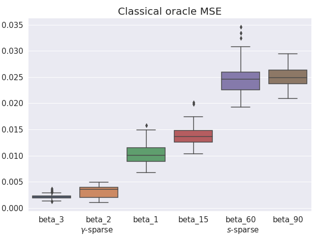
The plots are based on Monte Carlo simulations from model (1.1) with $p=n=1000$ and a signal $f^{*}$ , the sparsity of which is unknown to the methods. As benchmarks, we additionally provide the values of the risk at the classical oracle iteration $m^{\mathfrak{o}}:=\argmin_{m\geq 0}\|\widehat{F}^{(m)}-f^{*}\|_{n}^{2}$ and the default method LassoCV from the python library scikit-learn [18] based on 5-fold cross-validation. The exact specifications of the simulation are in Section 5. Table 1 contains the computation times for the different methods. The results suggest that sequential early stopping performs as well as established exhaustive model selection criteria at an immensely reduced computational cost, requiring only the computation of $\tau$ iterations of OMP.

The contribution of this paper is to provide rigorous theoretical guarantees that justify this statement. In the remainder of Section 1, we present our main results, which are a fully general oracle inequality for the empirical risk at $\tau$ and an optimal adaptation guarantee for the population risk in terms of the rates from Ing [12]. In Section 2, we study the stopped empirical risk in detail and provide precise bounds for important elementary quantities, which are used to extend our results to the population risk in Section 3. The analysis, which is conducted $\omega$ -pointwise on the underlying probability space, is able to avoid some of the saturation phenomena which occurred in previous works, see Blanchard et al. [3] and Celisse and Wahl [8] in particular. Both of our main theorems require access to a rate-optimal estimator $\widehat{\sigma}^{2}$ of $\|\varepsilon\|_{n}^{2}$ . Section 4 presents a noise estimation result which shows that such estimators do exist and can be computed efficiently. Section 5 provides a simulation study, which illustrates our main findings numerically. Finally, in the two-step procedure from (iv), we combine early stopping with a second model selection step over the iterations $m\leq\tau$ . This procedure, which empirically outperforms the others, inherits the guarantees for early stopping from our main results, while robustifying the methodology against deviations in the stopping time.

1.1 A general oracle inequality for the empirical risk

In order to state results for sequential early stopping of OMP in model (1.1), as minimal assumptions, we require that the rows $(X_{i})_{i\leq n}$ of the design matrix $\mathbf{X}=(X_{i}^{(j)})_{i\leq n,j\leq p}$ are independently and identically distributed such that $\mathbf{X}$ has full rank $n$ almost surely. We also require that the noise terms $(\varepsilon_{i})_{i\leq n}$ are independently and identically distributed and assume that, conditional on the design, a joint subgaussian parameter for the noise terms exists.

(A1)

(SubGE): Conditional on the design, the noise terms are centered subgaussians with a joint parameter $\overline{\sigma}^{2}>0$ , i.e., for all $i\leq n$ and $u\in\mathbb{R}$ ,

$\displaystyle\mathbb{E}(e^{u\varepsilon_{i}}|X_{i})$ $\displaystyle\leq e^{\frac{u^{2}\overline{\sigma}^{2}}{2}}\qquad\text{almost surely.}$

Complementary to $\overline{\sigma}^{2}$ , we set $\underline{\sigma}^{2}:=\text{Var}(\varepsilon_{1})$ .

By conditioning, we have $\underline{\sigma}^{2}=\mathbb{E}(\mathbb{E}(\varepsilon_{1}^{2}|X_{1}))\leq\overline{\sigma}^{2}$ . Assumption (SubGE) permits heteroscedastic error terms $(\varepsilon_{i})_{i\leq n}$ , allowing us to treat both regression and classification.

Example 1.1.

(a)

(Gaussian Regression): For $\varepsilon_{1},\dots\varepsilon_{n}\sim N(0,\sigma^{2})$ i.i.d., we have $\underline{\sigma}^{2}=\sigma^{2}=\overline{\sigma}^{2}$ .

(b)

(Classification): For classification, we consider i.i.d. observations

\displaystyle Y_{i}\sim\text{Ber}(f^{*}(X_{i})),\qquad i=1,\dots,n.

(1.3)

Then, the noise terms are given by $\varepsilon_{i}=Y_{i}-f^{*}(X_{i})$ with

\displaystyle\mathbb{E}(\varepsilon_{i}|X_{i})

\displaystyle=f^{*}(X_{i})(1-f^{*}(X_{i}))+(1-f^{*}(X_{i}))(-f^{*}(X_{i}))=0.

(1.4)

Conditional on the design, the noise is bounded by one. This implies that $\overline{\sigma}^{2}\leq 1$ .

For the asymptotic analysis, we assume that the observations stem from a sequence of models of the form (1.1), where $p=p^{(n)}\to\infty$ and $\log(p^{(n)})/n\to 0$ for $n\to\infty$ . We allow the quantities $\mathbf{X}=\mathbf{X}^{(n)},\beta^{*}=(\beta^{*})^{(n)}\text{ and }\varepsilon=\varepsilon^{(n)}$ to vary in $n$ . For notational convenience, we keep this dependence implicit.

In this setting, $L^{2}$ -boosting based on OMP is used to estimate $f^{*}$ and perform variable selection at the same time. Empirical correlations between data vectors are measured via the empirical inner product $\langle a,b\rangle_{n}:=n^{-1}\sum_{i=1}^{n}a_{i}b_{i}$ with norm $\|a\|_{n}:=\langle a,a\rangle_{n}^{1/2},$ for $a,b\in\mathbb{R}^{n}$ . By $\widehat{\Pi}_{J}:\mathbb{R}^{n}\to\mathbb{R}^{n},$ we denote the orthogonal projection with respect to $\langle\cdot,\cdot\rangle_{n}$ onto the span of the columns $\{X^{(j)}:j\in J\}$ of the design matrix. OMP is initialized at $\widehat{F}^{(0)}:=0$ and then iteratively selects the covariates $X^{(j)},j\leq p$ , which maximize the empirical correlation with the residuals $Y-\widehat{F}^{(m)}$ at the current iteration $m$ . The estimator is updated by projecting onto the subspace spanned by the selected covariates. Explicitly, the procedure is given by the following algorithm:

Algorithm 1 Orthogonal matching pursuit (OMP)

\widehat{F}^{(0)}\leftarrow 0,\widehat{J}_{0}\leftarrow\emptyset

2: for

m=0,1,2,\dots

\widehat{j}_{m+1}\leftarrow\argmax_{j\leq p}\Big|\Big\langle Y-\widehat{F}^{(m)},\frac{X^{(j)}}{\|X^{(j)}\|_{n}}\Big\rangle_{n}\Big|

\widehat{J}_{m+1}\leftarrow\widehat{J}_{m}\cup\big\{\widehat{j}_{m+1}\big\}

\widehat{F}^{(m+1)}\leftarrow\widehat{\Pi}_{\widehat{J}_{m+1}}Y

6: end for

Maximizing the empirical correlation between the residuals $Y-\widehat{F}^{(m)}$ and $X^{(\widehat{j}_{m+1})}$ at iteration $m$ is equivalent to minimizing $\|Y-\widehat{F}^{(m+1)}\|_{n}^{2}$ , i.e., OMP performs greedy optimization for the residual norm. It is therefore natural to stop this procedure at $\tau$ from Equation (1.2) when the residual norm reaches a critical value.

From a statistical perspective, we are interested in the risk of the estimators $\widehat{F}^{(m)},m\geq 0$ . Initially, we consider the empirical risk

\displaystyle\|\widehat{F}^{(m)}-f^{*}\|_{n}^{2}

\displaystyle=\|(I-\widehat{\Pi}_{m})f^{*}\|_{n}^{2}+\|\widehat{\Pi}_{m}\varepsilon\|_{n}^{2}=b_{m}^{2}+s_{m},

(1.5)

where we introduce the notation $\widehat{\Pi}_{m}:=\widehat{\Pi}_{\widehat{J}_{m}},b_{m}^{2}:=\|(I-\widehat{\Pi}_{m})f^{*}\|_{n}^{2}$ for the squared empirical bias and $s_{m}:=\|\widehat{\Pi}_{m}\varepsilon\|_{n}^{2}$ for the empirical stochastic error.¹¹ 1 In the term $b_{m}^{2}$ , we use the standard overloading of notation, letting $f^{*}$ denote $(f^{*}(X_{i}))_{i\leq n}$ , see Section 1.3. Note that at this point, we cannot simply take expectations, due to the non-linear, stochastic choice of $\widehat{J}_{m}$ . The definition of the orthogonal projections $(\widehat{\Pi}_{m})_{m\geq 0}$ with respect to $\langle\cdot,\cdot\rangle_{n}$ guarantees that the mappings $m\mapsto b_{m}^{2}$ and $m\mapsto s_{m}$ are monotonously decreasing and increasing, respectively.

This reveals the fundamental problem of selecting an iteration of the procedure in Algorithm 1. We need to iterate far enough to sufficiently reduce the bias, yet not too far as to blow up the stochastic error. For $m\geq n$ , we have $b_{m}^{2}=0\text{ but also }s_{m}=\|\varepsilon\|_{n}^{2}$ , which converges to $\underline{\sigma}^{2}$ by the law of large numbers. In particular, this means iterating Algorithm 1 indefinitely will not produce a consistent estimator of the unknown signal $f^{*}$ . Since the decay of the bias depends on $f^{*}$ , no a priori, i.e., data independent, choice of the iteration will perform well in terms of the risk uniformly over different realizations of $f^{*}$ . Therefore, Algorithm 1 needs to be combined with a data-driven choice $\widehat{m}$ of the effectively selected iteration, which is adaptive. This means either, without prior knowledge of $f^{*}$ , the choice $\widehat{m}$ satisfies an oracle inequality relating its performance to that of the ideal oracle iteration

\displaystyle m^{\mathfrak{o}}=m^{\mathfrak{o}}(f^{*}):=\argmin_{m\geq 0}\|\widehat{F}^{(m)}-f^{*}\|_{n}^{2}

(1.6)

or, in terms of convergence rates for the risk, $\widehat{m}$ performs optimally for multiple classes of signals without prior knowledge of the class to which the true signal $f^{*}$ belongs.

Our analysis in Section 2 shows that in order to derive such an adaptation result for the sequential early stopping time $\tau$ in Equation (1.2), ideally, the critical value $\kappa$ should be chosen depending on the iteration as

\displaystyle\kappa=\kappa_{m}=\|\varepsilon\|_{n}^{2}+\frac{C_{\tau}m\log p}{n},\qquad m\geq 0,

(1.7)

where $C_{\tau}\geq 0$ is a non-negative constant. Since the empirical noise level $\|\varepsilon\|_{n}^{2}$ is unknown, it has to be replaced by an estimator $\widehat{\sigma}^{2}$ and we redefine

\displaystyle\tau:=\inf\{m\geq 0:r_{m}^{2}\leq\kappa_{m}\}\qquad\text{ with }\qquad\kappa_{m}:=\widehat{\sigma}^{2}+\frac{C_{\tau}m\log p}{n},\qquad m\geq 0.

(1.8)

Our first main result is an oracle inequality for the stopped empirical risk at $\tau$ .

Theorem 1.2 (Oracle inequality for the empirical risk).

Under Assumption (SubGE), the empirical risk at the stopping time $\tau$ in Equation (1.8) with $C_{\tau}\geq 8\overline{\sigma}^{2}$ satisfies

	$\displaystyle\\|\widehat{F}^{(\tau)}-f^{*}\\|_{n}^{2}$	$\displaystyle\leq\min_{m\geq 0}\Big(7\\|\widehat{F}^{(m)}-f^{*}\\|_{n}^{2}+\frac{(8\overline{\sigma}^{2}+C_{\tau})m\log p}{n}\Big)+\|\widehat{\sigma}^{2}-\\|\varepsilon\\|_{n}^{2}\|$
		$\displaystyle\leq 7\\|\widehat{F}^{(m^{\mathfrak{o}})}-f^{*}\\|_{n}^{2}+\frac{(8\overline{\sigma}^{2}+C_{\tau})m^{\mathfrak{o}}\log p}{n}+\|\widehat{\sigma}^{2}-\\|\varepsilon\\|_{n}^{2}\|$

with probability converging to one.

The oracle inequality is completely general in the sense that no assumption on $f^{*}$ is required. In particular, the result also holds for non-sparse $f^{*}$ . The first term on the right-hand side involving the iteration $m^{\mathfrak{o}}$ from Equation (1.6) is of optimal order and the second term matches the upper bound for the empirical stochastic error at iteration $m^{\mathfrak{o}}$ we derive in Lemma 2.5. The last term is the absolute estimation error of $\widehat{\sigma}^{2}$ for the empirical noise level. The result is closely related to Theorem 3.3 in Blanchard et al. [3]. Whereas they state their oracle inequality in expectation, ours is formulated $\omega$ -pointwise on the underlying probability space, which is slightly stronger. In particular, this leads to the term $|\widehat{\sigma}^{2}-\|\varepsilon\|_{n}^{2}|$ in the inequality, which will be essential for the noise estimation problem, see Section 4.

1.2 Optimal adaptation for the population risk

The population counterpart of the empirical inner product is $\langle f,g\rangle_{L^{2}}:=\mathbb{E}(f(X_{1})g(X_{1}))$ with norm $\|f\|_{L^{2}}:=\langle f,f\rangle_{L^{2}}^{1/2}$ for functions $f,g\in L^{2}(\mathbb{P}^{X_{1}}),$ where $\mathbb{P}^{X_{1}}$ denotes the distribution of one observation of the covariates. Identifying $\widehat{F}^{(m)}$ with its corresponding function in the covariates, the population risk of the estimators is given by $\|\widehat{F}^{(m)}-f^{*}\|_{L^{2}}^{2},m\geq 0$ . Assuming that all of the covariates are square-integrable, for $J\subset\{1,\dots,p\}$ , let $\Pi_{J}:L^{2}(\mathbb{P}^{X_{1}})\to L^{2}(\mathbb{P}^{X_{1}})$ denote the orthogonal projection with respect to $\langle\cdot,\cdot\rangle_{L^{2}}$ onto the span of the covariates $\{X_{1}^{(j)}:j\in J\}$ . Setting $\Pi_{m}:=\Pi_{\widehat{J}_{m}}$ , the population risk decomposes into

\displaystyle\|\widehat{F}^{(m)}-f^{*}\|_{L^{2}}^{2}

\displaystyle=\|(I-\Pi_{m})f^{*}\|_{L^{2}}^{2}+\|\widehat{F}^{(m)}-\Pi_{m}f^{*}\|_{L^{2}}^{2}=B_{m}^{2}+S_{m},

(1.9)

where $B_{m}^{2}:a=\|(I-\Pi_{m})f^{*}\|_{L^{2}}^{2}$ is the squared population bias and $S_{m}:=\|\widehat{F}^{(m)}-\Pi_{m}f^{*}\|_{L^{2}}^{2}$ is the population stochastic error.

Note that $B_{m}^{2}$ and $S_{m}$ are not the exact population counterparts of the empirical quantities $b_{m}^{2}$ and $s_{m}$ , since we have to account for the difference between $\widehat{\Pi}_{m}$ and $\Pi_{m}$ . The challenge of selecting the iteration in Algorithm 1 discussed in the previous section is the same for the population risk. The mapping $m\mapsto B_{m}^{2}$ is monotonously decreasing, $S_{0}=0$ and $S_{m}$ approaches $\text{Var}(\varepsilon_{1})$ for $m\to\infty$ assuming that the difference between $\widehat{\Pi}_{m}$ and $\Pi_{m}$ becomes negligible. Due to this difference, however, the mapping $m\mapsto S_{m}$ is no longer guaranteed to be monotonous. Both $B_{m}$ and $S_{m}$ are still random quantities due to the randomness of $\widehat{J}_{m}$ .

In order to derive guarantees for the population risk, additional assumptions are required. We quantify the sparsity of the coefficients $\beta^{*}$ of $f^{*}$ :

(A2)

(Sparse): We assume one of the two following assumptions holds.

(i)

$\beta^{*}$ is $s$ -sparse for some $s\in\mathbb{N}_{0}$ , i.e., $\|\beta^{*}\|_{0}\leq s$ , where $\|\beta^{*}\|_{0}$ is the cardinality of the support $S:=\{j\leq p:|\beta^{*}_{j}|\neq 0\}$ . Additionally, we require that

\displaystyle s\|\beta^{*}\|_{1}^{2}=s\Big(\sum_{j=1}^{p}|\beta^{*}_{j}|\Big)^{2}=o\Big(\frac{n}{\log p}\Big),\quad\|f^{*}\|_{L^{2}}^{2}\leq C_{f^{*}}\quad\text{ and }\quad\min_{j\in S}|\beta^{*}_{j}|\geq\underline{\beta},

where $C_{f^{*}},\underline{\beta}>0$ are numerical constants.

(ii)

$\beta^{*}$ is $\gamma$ -sparse for some $\gamma\in[1,\infty)$ , i.e., $\|\beta^{*}\|_{2}\leq C_{\ell^{2}}$ and

\displaystyle\sum_{j\in J}|\beta_{j}^{*}|

\displaystyle\leq C_{\gamma}\Big(\sum_{j\in J}|\beta_{j}^{*}|^{2}\Big)^{\frac{\gamma-1}{2\gamma-1}}\qquad\text{ for all }J\subset\{1,\dots,p\},

where $C_{\ell^{2}},C_{\gamma}>0$ are numerical constants.

Assumptions like (Sparse) (i) are standard in the literature on high dimensional models, see e.g., Bühlmann and van de Geer [7]. Note that the conditions in (i) imply that $s=o((n/\log p)^{1/3})$ . (Sparse) (ii) encodes a decay of the coefficients $\beta^{*}$ . It includes several well known settings as special cases.

Example 1.3.

(a)

( $\ell^{1/\gamma}$ -boundedness): For $\gamma\in[1,\infty)$ and some $C_{\ell^{1/\gamma}}>0$ , let the coefficients satisfy $\sum_{j=1}^{p}|\beta^{*}_{j}|^{1/\gamma}\leq C_{\ell^{1/\gamma}}$ . Then, Hoelder’s inequality yields

	$\displaystyle\sum_{j\in J}\|\beta^{*}_{j}\|$	$\displaystyle=\sum_{j\in J}\|\beta^{}_{j}\|^{\frac{1}{2\gamma-1}}\|\beta^{}_{j}\|^{\frac{2\gamma-2}{2\gamma-1}}\leq\Big(\sum_{j\in J}\|\beta^{}_{j}\|^{\frac{1}{\gamma}}\Big)^{\frac{\gamma}{2\gamma-1}}\Big(\sum_{j\in J}\|\beta^{}_{j}\|^{2}\Big)^{\frac{\gamma-1}{2\gamma-1}}$		(1.10)
		$\displaystyle\leq(C_{\ell^{1/\gamma}})^{\frac{\gamma}{2\gamma-1}}\Big(\sum_{j\in J}\|\beta^{*}_{j}\|^{2}\Big)^{\frac{\gamma-1}{2\gamma-1}}\qquad\text{ for all }J\subset\{1,\dots,p\},$

i.e., Assumption (Sparse) (ii) is satisfied with $C_{\gamma}=(C_{\ell^{1/\gamma}})^{\frac{\gamma}{2\gamma-1}}$ . For $\gamma\to\infty$ , this approaches the setting in (i), in which the support $S$ is finite.

(b)

(Polynomial decay): For $\gamma\in(1,\infty)$ and $C_{\gamma}^{\prime}\geq c_{\gamma}^{\prime}>0$ , let the coefficients satisfy

\displaystyle c_{\gamma}^{\prime}j^{-\gamma}\leq|\beta^{*}_{(j)}|\leq C_{\gamma}^{\prime}j^{-\gamma}\qquad\qquad\text{ for all }j\leq p,

(1.11)

where $(\beta^{*}_{(j)})_{j\leq p}$ is a reordering of the $(\beta^{*}_{j})_{j\leq p}$ with decreasing absolute values. Then, Assumption (Sparse) (ii) is satisfied with $C_{\gamma}$ proportional to $C_{\gamma}^{\prime}(c_{\gamma}^{\prime})^{-(2\gamma-2)/(2\gamma-1)},$ see Lemma A1.2 of Ing [12].

For the covariance structure of the design, we assume subgaussianity and some additional boundedness conditions.

(A3)

(SubGD): The design variables are centered subgaussians in $\mathbb{R}^{p}$ with unit variance, i.e., there exists some $\rho>0$ such that for all $x\in\mathbb{R}^{p}\text{ with }\|x\|=1,$

\displaystyle\mathbb{E}e^{u\langle x,X_{1}\rangle}

\displaystyle\leq e^{\frac{u^{2}\rho^{2}}{2}},\quad u\in\mathbb{R}\qquad\text{ and }\qquad\text{Var}(X_{1}^{(j)})=1\quad\text{ for all }j\leq p.

Remark 1.4 (Inclusion of an Intercept).

Assumption (SubGD) still allows to include an intercept additional to the design variables. If the intercept is selected, we have just applied Algorithm 1 to the data $Y$ centered at their empirical mean for which (SubGD) is satisfied up to a negligible term. If it is not selected, the result is identical to applying the Algorithm without an intercept.

(A4)

(CovB): The complete covariance matrix $\Gamma:=\text{Cov}(X_{1})$ of one design observation is bounded from below, i.e., there exists some $c_{\lambda}>0$ such that the smallest eigenvalue of $\Gamma$ satisfies

$\displaystyle\lambda_{\min}(\Gamma)\geq c_{\lambda}>0.$ (1.12)

Further, we assume that there exists $C_{\text{Cov}}>0$ such that the partial population covariance matrices $\Gamma_{J}:=(\Gamma_{jk})_{j,k\in J},$ for $J\subset\{1,\dots,p\},$ satisfy

$\displaystyle\sup_{|J|\leq M_{n},k\not\in J}\|\Gamma^{-1}_{J}v_{k}\|_{1}<C_{\text{Cov}}$ (1.13)

with $M_{n}:=\sqrt{n/((\bar{\sigma}^{2}+\rho^{4})\log p)}$ , where $v_{k}:=(\text{Cov}(X_{1}^{(k)},X_{1}^{(j)}))_{j\in J}\in\mathbb{R}^{|J|}$ is the vector of covariances between the $k$ -th covariate and the covariates from the set $J$ .

$(\Gamma_{J}^{-1}v_{k})_{j\in J}$ is the vector of coefficients for the $X_{1}^{(j)},j\in J$ , in the conditional expectation $\mathbb{E}(X_{1}^{(k)}|X_{1}^{(j)},\\ j\in J)$ . $M_{n}$ will be the largest iteration of Algorithm 1 for which we need control over the covariance structure. Condition (1.13) imposes a restriction on the correlation between the covariates.

Example 1.5.

(a)

(Uncorrelated design): For $\Gamma=I_{p}$ , condition (1.13) is satisfied for any choice $C_{\text{Cov}}>0$ , since the left-hand side of the condition is zero.

(b)

(Bounded cumulative coherence): For $m\geq 0$ and $J\subset\{1,\dots,p\}$ , let

\displaystyle\mu_{1}(m):=\max_{k\leq p}\max_{|J|\leq m,k\not\in J}\sum_{j\in J}\text{Cov}(X_{1}^{(k)},X_{1}^{(j)})

(1.14)

be the cumulative coherence function. Then,

\displaystyle\sup_{|J|\leq M_{n},k\not\in J}\|\Gamma^{-1}_{J}v_{k}\|_{1}

\displaystyle\leq\sup_{|J|\leq M_{n},k\not\in J}\|\Gamma_{J}^{-1}\|_{1}\mu_{1}(M_{n}),

(1.15)

where $\|\Gamma_{J}^{-1}\|_{1}$ denotes the column sum norm. Under the assumption that both quantities on the right-hand side are bounded, condition (1.13) is satisfied. Under the stronger assumption that $\mu_{1}(M_{n})<1/2,$ it can be shown that condition (1.13) is satisfied with $C_{\text{Cov}}=1$ . This is the exact recovery condition in Theorem 3.5 of Tropp [23].

As in Ing [12], condition (1.13) guarantees that the coefficients $\beta((I-\Pi_{J})f^{*})$ of the population residual term $(I-\Pi_{J})f^{*}$ satisfy

	$\displaystyle\\|\beta((I-\Pi_{J})f^{})\\|_{1}=\\|\beta^{}-\beta(\Pi_{J}f^{})\\|_{1}\leq(C_{\text{Cov}}+1)\sum_{j\not\in J}\|\beta^{}_{j}\|$		(1.16)
	$\displaystyle\qquad\qquad\qquad\qquad\qquad\qquad\qquad\text{ for all }\|J\|\leq M_{n},$

where $J$ ranges over all subsets of $\{1,\dots,p\}$ . A derivation is stated in Lemma C.1. Equation (1.16) provides a uniform bound on the vector difference of the finite time predictor coefficients $\beta(\Pi_{J}f^{*})$ of $\Pi_{J}f^{*}$ and the infinite time predictor coefficients $\beta^{*}$ . In the literature on autoregressive modeling, such an inequality is referred to as a uniform Baxter’s inequality, see Ing [12] and the references therein, Baxter [2] and Meyer et al. [15].

Under Assumptions (A1) - (A4), explicit bounds for the population bias and the stochastic error are available. In the formulation of the results, the postpositioned “with probability converging to one” always refers to the whole statement including quantification over $m\geq 0$ , see also Section 1.3.

Lemma 1.6 (Bound for the population stochastic error, Ing [12]).

Under Assumptions (SubGE), (Sparse), (SubGD) and (CovB), there is a constant $C_{\text{Stoch}}>0$ such that

	$\displaystyle S_{m}\leq C_{\text{Stoch}}\begin{cases}\frac{(\overline{\sigma}^{2}+\\|\beta^{}\\|_{1}^{2}\rho^{4}\mathbf{1}\{m\leq\tilde{m}\})m\log p}{n},&\beta^{}\ s\text{-sparse},\\ \frac{(\overline{\sigma}^{2}+\rho^{4})m\log p}{n},&\beta^{*}\ \gamma\text{-sparse}\end{cases}$
	$\displaystyle\qquad\text{ for all }m\geq 0$

with probability converging to one, where $\tilde{m}=\inf\{m\geq 0:S\subset\widehat{J}_{m}\}$ .

The stochastic error grows linearly in $m$ , whereas, up to lower order terms, the bias decays exponentially when $\beta^{*}$ is $s$ -sparse and with a rate $m^{1-2\gamma}$ when $\beta^{*}$ is $\gamma$ -sparse.

Proposition 1.7 (Bound for the population bias, Ing [12]).

Under Assumptions (SubGE), (Sparse), (SubGD) and (CovB), there are constants $c_{\text{Bias}},C_{\text{Bias}}>0$ such that

	$\displaystyle B_{m}^{2}$	$\displaystyle\leq C_{\text{Bias}}\begin{cases}\\|f^{}\\|_{L^{2}}^{2}\exp\Big(\frac{-c_{\text{Bias}}m}{s}\Big)+\\|\beta^{}\\|_{1}^{2}\frac{s\log p}{n},&\beta^{}\ s\text{-sparse},\\ m^{1-2\gamma}+\Big(\frac{(\overline{\sigma}^{2}+\rho^{4})\log p}{n}\Big)^{1-\frac{1}{2\gamma}},&\beta^{}\ \gamma\text{-sparse}\\ \end{cases}$
		$\displaystyle\qquad\qquad\qquad\qquad\qquad\qquad\qquad\qquad\qquad\qquad\ \ \ \text{ for all }m\geq 0$

with probability converging to one. When $\beta^{*}$ is $s$ -sparse, on the corresponding event, there is a constant $C_{\text{supp}}>0$ such that $S\subset\widehat{J}_{C_{\text{supp}}s}$ .

Lemma 1.6 and Proposition 1.7 are essentially proven in Ing [12] but not stated explicitly. We include derivations in Appendix C to keep this paper self-contained.

Under $s$ -sparsity, the definition of the population bias guarantees that

\displaystyle B_{m}^{2}=0\qquad\text{ for all }m\geq C_{\text{supp}}s

(1.17)

with probability converging to one and under $\gamma$ -sparsity, the upper bounds from Lemma 1.6 and Proposition 1.7 balance at an iteration of size $(n/((\overline{\sigma}^{2}+\rho^{4})\log p))^{1/(2\gamma)}$ . We obtain that for

\displaystyle m^{*}_{s,\gamma}:=\begin{cases}C_{\text{supp}}s,&\beta^{*}\ s\text{-sparse},\\ \Big(\frac{n}{(\overline{\sigma}^{2}+\rho^{4})\log p}\Big)^{\frac{1}{2\gamma}},&\beta^{*}\ \gamma\text{-sparse},\\ \end{cases}

(1.18)

there exists a constant $C_{\text{Risk}}>0$ such that with probability converging to one, the population risk satisfies

\displaystyle\|\widehat{F}^{(m^{*}_{s,\gamma})}-f^{*}\|_{L^{2}}^{2}

\displaystyle\leq C_{\text{Risk}}\mathcal{R}(s,\gamma)

(1.19)

with the rates

\displaystyle\mathcal{R}(s,\gamma):=\begin{cases}\frac{\overline{\sigma}^{2}s\log p}{n},&\beta^{*}\ s\text{-sparse},\\ \Big(\frac{(\overline{\sigma}^{2}+\rho^{4})\log p}{n}\Big)^{1-\frac{1}{2\gamma}},&\beta^{*}\ \gamma\text{-sparse}.\end{cases}

(1.20)

In Lemmas 2.7 and 2.5, we show that the empirical quantities $b_{m}^{2}$ and $s_{m}$ satisfy bounds analogous to those stated in Proposition 1.7 and Lemma 1.6, such that also

\displaystyle\|\widehat{F}^{(m^{*}_{s,\gamma})}-f^{*}\|_{n}^{2}

\displaystyle\leq C_{\text{Risk}}\mathcal{R}(s,\gamma)

(1.21)

under the respective assumptions.

In general, we cannot expect to improve the rates $\mathcal{R}(s,\gamma)$ neither for the population nor for the empirical risk, see Ing [12] and our discussion in Section 2.3. Consequently, under $s$ -sparsity, we call a data-driven selection criterion $\widehat{m}$ adaptive to a parameter set $T\subset\mathbb{N}_{0}$ for one of the two risks, if the choice $\widehat{m}$ attains the rate $\mathcal{R}(s,\gamma)$ simultaneously over all $s$ -sparse signals $f^{*}$ with $s\in T$ , without any prior knowledge of $s$ . We call $\widehat{m}$ optimally adaptive, if the above holds for $T=\mathbb{N}_{0}$ . Under $\gamma$ -sparsity, we define adaptivity analogously with parametersets $T\subset[1,\infty)$ instead. Ideally, $\widehat{m}$ would be optimally adaptive both under $s$ - and $\gamma$ -sparsity even without any prior knowledge about what class of sparsity assumption is true for a given signal. Ing [12] proposes to determine $\widehat{m}$ via a high-dimensional Akaike criterion, which is in fact optimally adaptive for the population risk under both sparsity assumptions. In order to compute $\widehat{m}$ , however, the full iteration path of Algorithm 1 has to be computed as well.

Our second main result states that optimal adaptation is also achievable by a computationally efficient procedure, given by the early stopping rule in Equation (1.8). The proof of Theorem 1.8 is developed in Section 3.

Theorem 1.8 (Optimal adaptation for the population risk).

Under Assumptions (SubGE), (Sparse), (SubGD) and (CovB), choose $\widehat{\sigma}^{2}$ in Equation (1.8) such that there is a constant $C_{\text{Noise}}>0$ for which

\displaystyle|\widehat{\sigma}^{2}-\|\varepsilon\|_{n}^{2}|

\displaystyle\leq C_{\text{Noise}}\mathcal{R}(s,\gamma)

with probability converging to one. Then, the population risk at the stopping time in Equation (1.8) with $C_{\tau}=c(\overline{\sigma}^{2}+\rho^{4})$ for any $c>0$ satisfies

\displaystyle\|\widehat{F}^{(\tau)}-f^{*}\|_{L^{2}}^{2}

\displaystyle\leq C_{\text{PopRisk}}\mathcal{R}(s,\gamma)

with probability converging to one for a constant $C_{\text{PopRisk}}>0$ .

Under the additional Assumptions (Sparse), (SubGD) and (CovB), the bounds in Lemmas 2.7 and 2.5 also allow to translate Theorem 1.2 into optimal convergence rates by setting $m=m^{*}_{s,\gamma}$ from Equation (1.18):

Corollary 1.9 (Optimal adaptation for the empirical risk).

Under Assumptions (SubGE), (Sparse), (SubGD) and (CovB), the empirical risk at the stopping time in Equation (1.8) with $C_{\tau}=C(\overline{\sigma}^{2}+\rho^{4})$ with $C\geq 12$ satisfies

\displaystyle\|\widehat{F}^{(\tau)}-f^{*}\|_{n}^{2}

\displaystyle\leq C_{\text{EmpRisk}}\mathcal{R}(s,\gamma)+|\widehat{\sigma}^{2}-\|\varepsilon\|_{n}^{2}|,

with probability converging to one for a constant $C_{\text{EmpRisk}}>0$ .

In order for sequential early stopping to be adaptive over a parameter subset $T$ from $\mathbb{N}_{0}$ or $[1,\infty)$ , all of our results above require an estimator of the empirical noise level that attains the rates $\mathcal{R}(s,\gamma)$ for the absolute loss. In Proposition 4.2, we show that such an estimator does in fact exist, even for $T$ equal to $\mathbb{N}_{0}$ and $[1,\infty)$ . Together, this establishes that an optimally adaptive, fully sequential choice of the iteration in Algorithm 1 is possible. This is a strong positive result, given the fact that in previous settings adaptations has only been possible for restricted subsets of parameters, see Blanchard et al. [3] and Celisse and Wahl [8]. The two-step procedure, which we analyze in detail in Section 5, further robustifies this method against deviations in the stopping time and reduces the assumptions necessary for the noise estimation.

1.3 Further notation

We overload both the notation of the empirical and the population inner products with functions and vectors respectively, i.e., for $f,g:\mathbb{R}^{p}\to\mathbb{R},$ we set

\displaystyle\|f\|_{n}^{2}:=\frac{1}{n}\sum_{i=1}^{n}f(X_{i})^{2}\qquad\text{ and }\qquad\langle f,g\rangle_{n}:=\frac{1}{n}\sum_{i=1}^{n}f(X_{i})g(X_{i})

(1.22)

and also, e.g.,

\displaystyle\langle\varepsilon,f\rangle_{n}:=\frac{1}{n}\sum_{i=1}^{n}\varepsilon_{i}f(X_{i})\qquad\text{ or }\qquad\|Y\|_{L^{2}}^{2}:=\mathbb{E}Y_{1}^{2}.

(1.23)

Further, as in Bühlmann [6], for $j\leq p$ , we denote the $j$ -th coordinate projection as $g_{j}(x):=x^{(j)},x\in\mathbb{R}^{p},$ and vectors of dot products via

\displaystyle\langle\cdot,g_{J}\rangle_{n}:=(\langle\cdot,g_{j}\rangle_{n})_{j\in J}\in\mathbb{R}^{|J|}\qquad\text{ and }\qquad\langle\cdot,g_{J}\rangle_{L^{2}}:=(\langle\cdot,g_{j}\rangle_{L^{2}})_{j\in J}\in\mathbb{R}^{|J|}

(1.24)

for $J\subset\{1,\dots,p\}$ . This way, Equation (1.13) in Assumption (CovB) can be restated as

\displaystyle\sup_{|J|\leq M_{n},k\not\in J}\|\Gamma_{J}^{-1}\langle g_{k},g_{J}\rangle_{L^{2}}\|_{1}\leq C_{\text{Cov}}.

(1.25)

Analogously to the population covariance matrix $\Gamma=(\langle g_{j},g_{k}\rangle_{L^{2}})_{j,k\leq p}$ , we define the empirical covariance matrix $\widehat{\Gamma}:=(\langle g_{j},g_{k}\rangle_{n})_{j,k\leq p}$ . Using the same notation for partial matrices as in Assumption (CovB) and $X^{(J)}=(X_{i}^{(j)})_{i\leq n,j\in J}\in\mathbb{R}^{n\times|J|}$ , the projections $\widehat{\Pi}_{J}$ and $\Pi_{J}$ can be written as

	$\displaystyle\widehat{\Pi}_{J}:\mathbb{R}^{n}\to\mathbb{R}^{n},\qquad\qquad\qquad\ \ \ \widehat{\Pi}_{J}y:$	$\displaystyle=(X^{(J)})^{\top}\widehat{\Gamma}_{J}^{-1}\langle y,g_{J}\rangle_{n},$		(1.26)
	$\displaystyle\Pi_{J}:L^{2}(\mathbb{P}^{X_{1}})\to L^{2}(\mathbb{P}^{X_{1}}),\qquad\Pi_{J}h:$	$\displaystyle=g_{J}^{\top}\Gamma_{J}^{-1}\langle h,g_{J}\rangle_{L^{2}}$

for $J\subset\{1,\dots,p\}$ .

At points where we switch between a linear combination $f$ of the columns of the design and its coefficients, we introduce the notation $\beta(f)$ . We use this, e.g., for the coefficients of the population residual function $\beta((I-\Pi_{m})f^{*})$ as in Equation (1.16). For coefficients $\beta\in\mathbb{R}^{p}$ , we also use the general set notation $\beta_{J}:=(\beta_{j})_{j\in J}\in\mathbb{R}^{|J|}$ for $J\subset\{1,\dots,p\}$ .

Throughout the paper, variables $c>0$ and $C>0$ denote small and large constants respectively. They may change from line to line and can depend on constants defined in our assumptions. They are, however, independent of $n,\overline{\sigma}^{2}$ and $\rho^{2}$ .

Many statements in our results are formulated with a postpositioned “with probability converging to one”. This always refers to the whole statement including quantifiers. E.g. in Lemma 2.5, the result is to be read as: There exists an event with probability converging to one on which for all iterations $m\geq 0$ , the inequality $s_{m}\leq C\overline{\sigma}^{2}m\log(p)/n$ is satisfied.

2 Empirical risk analysis

Since the stopping time $\tau$ in Equation (1.2) is defined in terms of the squared empirical residual norm $r_{m}^{2}m\geq 0$ , its functioning principles are initially best explained by analyzing the stopped empirical risk $\|\widehat{F}^{(\tau)}-f^{*}\|_{n}^{2}$ . We begin by formulating an intuition for why $\tau$ is adaptive.

2.1 An intuition for sequential early stopping

Ideally, an adaptive choice $\widehat{m}$ of the iteration in Algorithm 1 would approximate the classical oracle iteration $m^{\mathfrak{o}}$ from Equation (1.6), which minimizes the empirical risk. The sequential stopping time $\tau$ , however, does not have a direct connection to $m^{\mathfrak{o}}$ . In fact, its sequential definition guarantees that $\tau$ does not incorporate information about the squared bias $b_{m}^{2}$ for iterations $m>\tau$ . Instead, $\tau$ mimics the balanced oracle iteration

\displaystyle m^{\mathfrak{b}}=m^{\mathfrak{b}}(f^{*}):=\inf\{m\geq 0:b_{m}^{2}\leq s_{m}\}.

(2.1)

Fortunately, the empirical risk at $m^{\mathfrak{b}}$ is essentially optimal up to a small discretization error, which opens up the possibility of sequential adaptation in the first place.

Lemma 2.1 (Optimality of the balanced oracle).

The empirical risk at the balanced oracle iteration $m^{\mathfrak{b}}$ satisfies

\displaystyle\|\widehat{F}^{(m^{\mathfrak{b}})}-f^{*}\|_{n}^{2}

\displaystyle\leq 2\|\widehat{F}^{(m^{\mathfrak{o}})}-f^{*}\|_{n}^{2}+\Delta(s_{m^{\mathfrak{b}}})=2\min_{m\geq 0}\|\widehat{F}^{(m)}-f^{*}\|_{n}^{2}+\Delta(s_{m^{\mathfrak{b}}}),

where $\Delta(s_{m}):=s_{m}-s_{m-1}$ is the discretization error of the empirical stochastic error at $m$ .

Proof.

If $m^{\mathfrak{b}}>m^{\mathfrak{o}}$ , then the definition of $m^{\mathfrak{b}}$ and the monotonicity of $m\mapsto b_{m}^{2}$ yield

	$\displaystyle\\|\widehat{F}^{(m^{\mathfrak{b}})}-f^{*}\\|_{n}^{2}$	$\displaystyle=b_{m^{\mathfrak{b}}}^{2}+s_{m^{\mathfrak{b}}}\leq 2b_{m^{\mathfrak{b}}}^{2}+\Delta(s_{m^{\mathfrak{b}}})\leq 2b_{m^{\mathfrak{o}}}^{2}+\Delta(s_{m^{\mathfrak{b}}})$		(2.2)
		$\displaystyle\leq 2\\|\widehat{F}^{(m^{\mathfrak{o}})}-f^{*}\\|_{n}^{2}+\Delta(s_{m^{\mathfrak{b}}}).$

Otherwise, if $m^{\mathfrak{b}}\leq m^{\mathfrak{o}}$ , then analogously, the monotonicity of $m\mapsto s_{m}$ yields $\|\widehat{F}^{(m^{\mathfrak{b}})}-f^{*}\|_{n}^{2}\leq 2s_{m^{\mathfrak{b}}}\leq 2\|\widehat{F}^{(m^{\mathfrak{o}})}-f^{*}\|_{n}^{2}$ . ∎

The connection between $\tau$ and $m^{\mathfrak{b}}$ can be seen by decomposing the squared residual norm $r_{m}^{2}$ into

	$\displaystyle r_{m}^{2}$	$\displaystyle=\\|(I-\widehat{\Pi}_{m})f^{}\\|_{n}^{2}+2\langle(I-\widehat{\Pi}_{m})f^{},\varepsilon\rangle_{n}+\\|(I-\widehat{\Pi}_{m})\varepsilon\\|_{n}^{2}$		(2.3)
		$\displaystyle=b_{m}^{2}+2c_{m}+\\|\varepsilon\\|_{n}^{2}-s_{m}$

with the cross term

\displaystyle c_{m}:=\langle(I-\widehat{\Pi}_{m})f^{*},\varepsilon\rangle_{n},\qquad m\geq 0.

(2.4)

Indeed, Equation (2.3) yields that the stopping condition $r_{m}^{2}\leq\kappa$ is equivalent to

\displaystyle b_{m}^{2}+2c_{m}

\displaystyle\leq s_{m}+\kappa-\|\varepsilon\|_{n}^{2}.

(2.5)

Assuming that $c_{m}$ can be treated as a lower order term, this implies that, up to the difference $\kappa-\|\varepsilon\|_{n}^{2}$ , $\tau$ behaves like $m^{\mathfrak{b}}$ .

The connection between a discrepancy-type stopping rule and a balanced oracle was initially drawn in Blanchard et al. [3, 4]. Whereas their oracle quantities were defined in terms of non-random population versions of bias and variance, ours have to be defined $\omega$ -pointwise on the underlying probability space. This is owed to the fact that, even conditional on the design $\mathbf{X}$ , the squared bias $b_{m}^{2}$ is still a random quantity due to the random selection of $\widehat{J}_{m}$ in Algorithm 1. This is a subtle but important distinction, which leads to a substantially different analysis.

2.2 A general oracle inequality

In this section, we derive the first main result in Theorem 1.2. As in Blanchard et al. [3], the key ingredient is that via the squared residual norm $r_{m}^{2},m\geq 0$ , the stopped estimator $\widehat{F}^{(\tau)}$ can be compared with any other estimator $\widehat{F}^{(m)}$ in empirical norm. Note that the statement in Lemma 2.2 is completely deterministic.

Lemma 2.2 (Empirical norm comparison).

For any $m\geq 0$ , the stopped estimator $\widehat{F}^{(\tau)}$ with $\tau$ from Equation (1.2) satisfies

	$\displaystyle\\|\widehat{F}^{(\tau)}-\widehat{F}^{(m)}\\|_{n}^{2}$	$\displaystyle\leq\\|\widehat{F}^{(m)}-f^{*}\\|_{n}^{2}+2\|c_{m}\|$
		$\displaystyle+(\kappa-\\|\varepsilon\\|_{n}^{2})\mathbf{1}\{\tau<m\}+(\\|\varepsilon\\|_{n}^{2}+\Delta(r_{\tau}^{2})-\kappa)\mathbf{1}\{\tau>m\},$

where $c_{m}$ is the cross term from Equation (2.4) and $\Delta(r_{m}^{2}):=r_{m}^{2}-r_{m-1}^{2}$ is the discretization error of the squared residual norm at $m$ .

Proof.

Fix $m\geq 0$ . We have

	$\displaystyle\\|\widehat{F}^{(\tau)}-\widehat{F}^{(m)}\\|_{n}^{2}$	$\displaystyle=\\|Y-\widehat{F}^{(\tau)}+\widehat{F}^{(m)}-Y\\|_{n}^{2}=r_{\tau}^{2}-2\langle(I-\widehat{\Pi}_{\tau})Y,(I-\widehat{\Pi}_{m})Y\rangle_{n}+r_{m}^{2}$
		$\displaystyle=(r_{m}^{2}-r_{\tau}^{2})\mathbf{1}\{\tau>m\}+(r_{\tau}^{2}-r_{m}^{2})\mathbf{1}\{\tau<m\}.$		(2.6)

On $\{\tau>m\}$ , we use the definition of $\tau$ in Equation (1.2) to estimate

	$\displaystyle r_{m}^{2}-r_{\tau}^{2}$	$\displaystyle\leq r_{m}^{2}-\kappa+\Delta(r_{\tau}^{2})=b_{m}^{2}+2c_{m}+\\|\varepsilon\\|_{n}^{2}-s_{m}-\kappa+\Delta(r_{\tau}^{2})$		(2.7)
		$\displaystyle\leq\\|\widehat{F}^{(m)}-f^{*}\\|_{n}^{2}+2c_{m}+\\|\varepsilon\\|_{n}^{2}-\kappa+\Delta(r_{\tau}^{2}).$

On $\{\tau\leq m\}$ , analogously, we obtain $r_{\tau}^{2}-r_{m}^{2}\leq\|\widehat{F}^{(m)}-f^{*}\|_{n}^{2}-2c_{m}+\kappa-\|\varepsilon\|_{n}^{2},$ which finishes the proof. ∎

In order to translate this norm comparison to an oracle inequality, it suffices to control the cross term and the discretization error of the residual norm. This is already possible under Assumption (SubGE). The proof of Lemma 2.3 is deferred to Appendix B.

Lemma 2.3 (Bounds for the cross term and the discretization error).

Under Assumption (SubGE), the following statements hold:

(i)

With probability converging to one, the cross term satisfies

$\displaystyle|c_{m}|$ $\displaystyle\leq b_{m}\sqrt{\frac{4\overline{\sigma}^{2}(m+1)\log p}{n}}\qquad\text{ for all }m\geq 0.$

(ii)

With probability converging to one, the discretization error of the squared residual norm satisfies

\displaystyle\Delta(r_{m}^{2})

\displaystyle\leq 2b_{m-1}^{2}+\frac{8\overline{\sigma}^{2}m\log p}{n}\qquad\text{ for all }m\geq 1.

Together, Lemmas 2.2 and 2.3 motivate the choice $\kappa=\kappa_{m}$ in Equation (1.8), where the additional term $C_{\tau}m\log(p)/n$ accounts for the discretization error of the residuals norm. With this choice of $\kappa$ , Lemma 2.2 yields for any fixed $m\geq 0$ that

$\displaystyle\\|\widehat{F}^{(\tau)}-f^{*}\\|_{n}^{2}$	$\displaystyle\leq 2(\\|\widehat{F}^{(\tau)}-\widehat{F}^{(m)}\\|_{n}^{2}+\\|\widehat{F}^{(m)}-f^{*}\\|_{n}^{2})$	(2.8)
	$\displaystyle\leq 2\big(2\\|\widehat{F}^{(m)}-f^{*}\\|_{n}^{2}+2\|c_{m}\|+(\kappa_{\tau}-\\|\varepsilon\\|_{n}^{2})\mathbf{1}\{\tau<m\}.$
	$\displaystyle\qquad\ \ \quad\qquad\qquad\qquad\qquad\ \ +(\\|\varepsilon\\|_{n}^{2}+\Delta(r_{\tau}^{2})-\kappa_{\tau})\mathbf{1}\{\tau>m\}\big).$

Under Assumption (SubGE), with probability converging to one, the estimates from Lemma 2.3 then imply that on $\{\tau<m\}$ ,

\displaystyle\|\widehat{F}^{(\tau)}-f^{*}\|_{n}^{2}

\displaystyle\leq 6\|\widehat{F}^{(m)}-f^{*}\|_{n}^{2}+\frac{(8\overline{\sigma}^{2}+C_{\tau})m\log p}{n}+\widehat{\sigma}^{2}-\|\varepsilon\|_{n}^{2},

(2.9)

using that $4(m+1)\leq 8m$ . Analogously, on $\{\tau>m\}$ , we obtain

\displaystyle\|\widehat{F}^{(\tau)}-f^{*}\|_{n}^{2}

\displaystyle\leq 7\|\widehat{F}^{(m)}-f^{*}\|_{n}^{2}+\frac{8\overline{\sigma}^{2}m\log p}{n}+\frac{(8\overline{\sigma}^{2}-C_{\tau})\tau\log p}{n}+\|\varepsilon\|_{n}^{2}-\widehat{\sigma}^{2},

(2.10)

where we have used that $b_{\tau-1}^{2}\leq b_{m}^{2}$ . Combining the events and taking the infimum over $m\geq 0$ yields the result in Theorem 1.2. We reiterate that here, it is the $\omega$ -pointwise analysis that preserves the term $|\widehat{\sigma}^{2}-\|\varepsilon\|_{n}^{2}|$ in the result.

2.3 Explicit bounds for empirical quantities

In order to derive a convergence rate from Theorem 1.2, we need explicit bounds for the empirical quantities involved. These will also be essential for the analysis of the stopped population risk. We begin by establishing control over the most basic quantities.

Lemma 2.4 (Uniform bounds in high probability).

Under Assumptions (SubGE) and (SubGD), the following statements hold:

(i)

There exists some $C_{g}>0$ such that with probability converging to one,

\displaystyle\sup_{j,k\leq p}|\langle g_{j},g_{k}\rangle_{n}-\langle g_{j},g_{k}\rangle_{L^{2}}|\leq C_{g}\sqrt{\frac{\rho^{4}\log p}{n}}.

(ii)

There exists some $C_{\varepsilon}>0$ such that with probability converging to one,

$\displaystyle\sup_{j\leq p}|\langle\varepsilon,g_{j}\rangle_{n}|\leq C_{\varepsilon}\sqrt{\frac{\overline{\sigma}^{2}\log p}{n}}.$

(iii)

There exists some $C_{\Gamma}>0$ such that for any fixed $c_{\text{Cov}}>0$ ,

\displaystyle\sup_{|J|\leq c_{\text{Cov}}n/\log p}\frac{\|\widehat{\Gamma}_{J}-\Gamma_{J}\|_{\text{op}}}{\rho^{2}}\leq c_{\text{Cov}}C_{\Gamma}

with probability converging to one.

(iv)

There exist $c_{\text{Cov}},C_{\Gamma^{-1}}>0$ such that with probability converging to one,

$\displaystyle\sup_{|J|\leq c_{\text{Cov}}n/\log p}\|\widehat{\Gamma}_{J}^{-1}\|_{\text{op}}\leq C_{\Gamma^{-1}}.$

Some version of this is needed in all results for $L^{2}$ -boosting in high-dimensional models, see Lemma 1 in Bühlmann [6], Lemma A.2 in Ing and Lai [13] or Assumptions (A1) and (A2) in Ing [12]. A proof for our setting is detailed in Appendix B. Note that Lemma 2.4 (iii) and (iv) improve the control to subsets $J$ with cardinality of order up to $n/\log p$ from Lemma A.2 in Ing and Lai [13], where only subsets of order $\sqrt{n/\log p}$ could be handled. For our results, we only need that $M_{n}\leq c_{\text{Cov}}n/\log p$ for $n$ sufficiently large, however, this could open up further research into the setting where $\gamma\in(1/2,1)$ , i.e., when $m^{*}_{s,\gamma}$ can be of order $n/\log p$ , see also Barron et al. [1].

From Lemma 2.4, we obtain that the empirical stochastic error $s_{m}$ satisfies a similar upper bound as its population counterpart $S_{m}$ .

Lemma 2.5 (Bound for the empirical stochastic error).

Under Assumptions (SubGE) and (SubGD), the empirical stochastic error satisfies

\displaystyle s_{m}

\displaystyle\leq C\frac{\overline{\sigma}^{2}m\log p}{n}\qquad\text{ for all }m\geq 0

with probability converging to one.

Proof.

For $m\leq c_{\text{iter}}n/\log p$ , using the notation from Equation (1.26), we can write

	$\displaystyle s_{m}$	$\displaystyle=\langle\varepsilon,\widehat{\Pi}_{m}\varepsilon\rangle_{n}=\langle\varepsilon,g_{\widehat{J}_{m}}^{\top}\widehat{\Gamma}_{\widehat{J}_{m}}^{-1}\langle\varepsilon,g_{\widehat{J}_{m}}\rangle_{n}\rangle_{n}\leq\\|\widehat{\Gamma}_{\widehat{J}_{m}}^{-1}\langle\varepsilon,g_{\widehat{J}_{m}}\rangle_{n}\\|_{1}\sup_{j\leq p}\|\langle\varepsilon,g_{j}\rangle_{n}\|$		(2.11)
		$\displaystyle\leq\sqrt{m}\\|\widehat{\Gamma}_{\widehat{J}_{m}}^{-1}\langle\varepsilon,g_{\widehat{J}_{m}}\rangle_{n}\\|_{2}\sup_{j\leq p}\|\langle\varepsilon,g_{j}\rangle_{n}\|\leq\\|\widehat{\Gamma}_{\widehat{J}_{m}}^{-1}\\|_{\text{op}}m\sup_{j\leq p}\|\langle\varepsilon,g_{j}\rangle_{n}\|^{2}.$

This yields the result for $m\leq M_{n}^{2}$ by taking the supremum and applying the bounds from Lemma 2.4 (ii) and (iv). For $m>c_{\text{iter}}n/\log p$ , the bound is also satisfied, since $s_{m}\leq\|\varepsilon\|_{n}^{2}\leq C\text{Var}(\varepsilon_{1})=C\underline{\sigma}^{2}\leq C\overline{\sigma}^{2}$ with probability one. ∎

In order to relate the empirical bias to the population bias, we use a norm change inequality from Ing [12], which we extend to the $s$ -sparse setting. A complete derivation, which is based on the uniform Baxter inequality in (1.16), is stated in Appendix C.

Proposition 2.6 (Fast norm change for the bias).

Under Assumptions (Sparse) and (CovB), the squared population bias $B_{m}^{2}=\|(I-\Pi_{m})f^{*}\|_{L^{2}}^{2}$ satisfies the norm change inequality

		$\displaystyle\ \ \ \ \|\\|(I-\Pi_{m})f^{}\\|_{n}^{2}-\\|(I-\Pi_{m})f^{}\\|_{L^{2}}^{2}\|$
		$\displaystyle\leq C\begin{cases}(s+m)\\|(I-\Pi_{m})f^{}\\|_{L^{2}}^{2}\sup_{j,k\leq p}\|\langle g_{j},g_{k}\rangle_{n}-\langle g_{j},g_{k}\rangle_{L^{2}}\|,&\beta^{}\ s\text{-sparse},\\ \big(\\|(I-\Pi_{m})f^{}\\|_{L^{2}}^{2}\big)^{\frac{2\gamma-2}{2\gamma-1}}\sup_{j,k\leq p}\|\langle g_{j},g_{k}\rangle_{n}-\langle g_{j},g_{k}\rangle_{L^{2}}\|,&\beta^{}\ \gamma\text{-sparse}\\ \end{cases}$

for any $m\leq M_{n}$ and $n$ large enough.

Proposition 2.6 will appear again in analyzing the stopping condition (2.5) in Section 3. Initially, it guarantees that the squared empirical bias $b_{m}^{2}$ satisfies the same bound as its population counterpart $B_{m}^{2}$ .

Lemma 2.7 (Bound for the empirical bias).

Under assumptions (SubGE), (Sparse), (SubGD) and (CovB), the squared empirical bias satisfies

	$\displaystyle b_{m}^{2}$	$\displaystyle\leq C\begin{cases}\\|f^{}\\|_{L^{2}}^{2}\exp\Big(\frac{-c_{\text{Bias}}m}{s}\Big)+\\|\beta^{}\\|_{1}^{2}\frac{s\log p}{n},&\beta^{}\ s\text{-sparse},\\ m^{1-2\gamma}+\Big(\frac{(\overline{\sigma}^{2}+\rho^{4})\log p}{n}\Big)^{1-1/(2\gamma)},&\beta^{}\ \gamma\text{-sparse}\\ \end{cases}$
		$\displaystyle\qquad\qquad\qquad\qquad\qquad\qquad\qquad\qquad\qquad\qquad\text{ for all }m\geq 0$

with probability converging to one.

Proof.

For a fixed $m\leq M_{n}$ and $n$ large enough, Proposition 2.6 yields the estimate

$\displaystyle b_{m}^{2}$	$\displaystyle=\\|(I-\widehat{\Pi}_{m})f^{}\\|_{n}^{2}\leq\\|(I-\Pi_{m})f^{}\\|_{n}^{2}$	(2.12)
	$\displaystyle\leq\\|(I-\Pi_{m})f^{*}\\|_{L^{2}}^{2}$
	$\displaystyle+C\begin{cases}(s+m)\\|(I-\Pi_{m})f^{}\\|_{L^{2}}^{2}\sup_{j,k\leq p}\|\langle g_{j},g_{k}\rangle_{n}-\langle g_{j},g_{k}\rangle_{L^{2}}\|,&\beta^{}\ s\text{-sparse},\\ \big(\\|(I-\Pi_{m})f^{}\\|_{L^{2}}^{2}\big)^{\frac{2\gamma-2}{2\gamma-1}}\sup_{j,k\leq p}\|\langle g_{j},g_{k}\rangle_{n}-\langle g_{j},g_{k}\rangle_{L^{2}}\|,&\beta^{}\ \gamma\text{-sparse}.\\ \end{cases}$

Applying Lemma 2.4 (i) and Proposition 1.7 then yields the result for $m\leq M_{n}$ . The monotonicity of $m\mapsto b_{m}^{2}$ implies that the claim is also true for any $m>M_{n}$ under $\gamma$ -sparsity. Under $s$ -sparsity, $b_{m}^{2}=0$ for all $m\geq C_{\text{supp}}s$ with $s=o((n/\log p)^{1/3})$ . This finishes the proof. ∎

Analogous to Equation (1.19), Lemmas 2.5 and 2.7 imply that at iteration $m^{*}_{s,\gamma}$ from Equation (1.18), the empirical risk satisfies the bound

\displaystyle\|\widehat{F}^{(m^{*}_{s,\gamma})}-f^{*}\|_{n}^{2}

\displaystyle\leq C\mathcal{R}(s,\gamma)

(2.13)

with probability converging to one. This yields the result Corollary 1.9. For the empirical risk, we can also argue precisely that such a result cannot be improved upon:

Remark 2.8 (Optimality of the rates).

For simplicity, we consider $p=n$ , a fixed, orthogonal (with respect to $\langle\cdot,\cdot\rangle_{n}$ ) design matrix $\mathbf{X}$ and $\varepsilon\sim N(0,\sigma^{2}I_{n})$ . Conceptually, $\rho^{2}=0$ in this setting. When $\beta^{*}$ is $s$ -sparse, the squared empirical bias satisfies

\displaystyle b_{m}^{2}

\displaystyle=\|(I-\widehat{\Pi}_{m})f^{*}\|_{n}^{2}\geq\|\beta(\widehat{\Pi}_{m}f^{*})-\beta^{*}\|_{2}^{2}\geq\underline{\beta}^{2}

(2.14)

for any $m\leq s$ . Similarly, when $\beta^{*}$ is $\gamma$ -sparse,

\displaystyle b_{m}^{2}

\displaystyle=\|(I-\widehat{\Pi}_{m})f^{*}\|_{n}^{2}\geq\|\beta^{*}_{m\text{-term}}-\beta^{*}\|_{2}^{2},

(2.15)

where $\beta^{*}_{m\text{-term}}$ is the best $m$ -term approximation of $\beta^{*}$ with respect to the euclidean norm. For $\beta^{*}$ with polynomial decay as in Equation (1.11), the right-hand side in Equation (2.15) is larger than $cm^{1-2\gamma}$ , see e.g., Lemma A.3 in Ing [12].

Conversely, for $f^{*}=0$ , the greedy procedure in Algorithm 1 guarantees that

\displaystyle s_{m}

\displaystyle=\|\widehat{\Pi}_{m}\varepsilon\|_{n}^{2}=\frac{1}{n}\sum_{j=1}^{m}Z_{(n-j+1)}^{2}\geq\frac{mZ_{(p-m+1)}^{2}}{n},

(2.16)

where $Z_{(j)}$ denotes the $j$ -th order statistic of the $Z_{j}:=\langle X^{(j)},\varepsilon\rangle_{n}$ , $j\leq p$ , which are again independent, identically distributed Gaussians with variance $\sigma^{2}$ . Noting that $s=o((n/\log p)^{1/3})$ , for both $m=s$ and $m=(n/(\sigma^{2}\log p))^{1/(2\gamma)}$ , the order statistic $Z_{p-m+1}$ is larger than $c\sqrt{\sigma^{2}\log p}$ with probability converging to one, see Lemma B.2. Consequently, by distinguishing the cases where $m$ is smaller or greater than $s$ under $s$ -sparsity and the cases where $m$ is smaller or greater than $(n/(\sigma^{2}\log p))^{1/(2\gamma)}$ under $\gamma$ -sparsity, we obtain

\displaystyle\inf_{m\geq 0}\sup_{f^{*}}\|\widehat{F}^{(m)}-f^{*}\|_{n}^{2}\geq c\begin{cases}\frac{\sigma^{2}s\log p}{n},&\beta^{*}\ s\text{-sparse},\\ \Big(\frac{\sigma^{2}\log p}{n}\Big)^{1-\frac{1}{2\gamma}},&\beta^{*}\ \gamma\text{-sparse}\end{cases}

(2.17)

with probability converging to one, where the infimum is taken over either all $f^{*}$ satisfying (Sparse) (i) or over all $f^{*}$ satisfying (Sparse) (ii).

3 Population risk analysis

In this section, we analyze the stopped population risk $\|\widehat{F}^{(\tau)}-f^{*}\|_{L^{2}}^{2}$ with $\tau$ from Equation (1.8). Unlike the empirical risk, the population risk cannot be expressed in terms of the residuals straight away. Instead, we examine the stopping condition $r_{m}^{2}\leq\kappa_{m}$ , i.e.,

\displaystyle b_{m}^{2}+2c_{m}

\displaystyle\leq\widehat{\sigma}^{2}-\|\varepsilon\|_{n}^{2}+\frac{C_{\tau}m\log p}{n}+s_{m}.

(3.1)

We show separately that for a suitable choice of $\widehat{\sigma}^{2}$ , condition (3.1) guarantees that $\tau$ stops neither too early nor too late. In combination, this yields Theorem 1.8. For the analysis, it becomes essential that we have access to the fast norm change for the population residual term $(I-\Pi_{m})f^{*}$ from Proposition 2.6, which guarantees that empirical and population norm remain of the same size until the squared population bias reaches the optimal rate $\mathcal{R}(s,\gamma)$ . This control is not already readily available by standard tools, e.g., Wainwright [26].

3.1 No stopping too early

The sequential procedure stops too early if the squared population bias $B_{m}^{2}=\|(I-\Pi_{m})f^{*}\|_{L^{2}}^{2}$ has not reached the optimal rate of convergence yet, i.e., $\tau<\tilde{m}_{s,\gamma,G}$ , where

\displaystyle\tilde{m}_{s,\gamma,G}:=\begin{cases}\inf\{m\geq 0:S\subset\widehat{J}_{m}\},&\beta^{*}\ s\text{-sparse},\\ \inf\Big\{m\geq 0:\|(I-\Pi_{m})f^{*}\|_{L^{2}}^{2}\leq G\Big(\frac{(\overline{\sigma}^{2}+\rho^{4})\log p}{n}\Big)^{1-\frac{1}{2\gamma}}\Big\},&\beta^{*}\ \gamma\text{-sparse}\end{cases}

(3.2)

for any constant $G>0$ . Note that under (CovB), for $s$ -sparse $\beta^{*}$ ,

\displaystyle B_{m}^{2}

\displaystyle=\|(I-\Pi_{m})f^{*}\|_{L^{2}}^{2}\begin{cases}\geq c_{\lambda}\|\tilde{\beta}\|_{2}^{2}\geq c_{\lambda}\underline{\beta}^{2},&m<\tilde{m}_{s,\gamma,G},\\ =0,&m\geq\tilde{m}_{s,\gamma,G}.\end{cases}

(3.3)

Therefore, a condition for stopping too early is given by

\displaystyle\exists m<\tilde{m}_{s,\gamma,G}:b_{m}^{2}+2c_{m}

\displaystyle\leq\widehat{\sigma}^{2}-\|\varepsilon\|_{n}^{2}+\frac{C_{\tau}m\log p}{n}+s_{m},

(3.4)

where we may vary $G>0$ .

Using the norm change inequality for the bias in Proposition 2.6, we can derive that the left-hand side of condition (3.4) is of the same order as $B_{m}^{2}$ , i.e.,

\displaystyle b_{m}^{2}+2c_{m}

\displaystyle\geq\begin{cases}\frac{c_{\lambda}}{8}\underline{\beta}^{2},&\beta^{*}\ s\text{-sparse},\\ \frac{G}{8}\Big(\frac{(\overline{\sigma}^{2}+\rho^{4})\log p}{n}\Big)^{1-\frac{1}{2\gamma}},&\beta^{*}\ \gamma\text{-sparse}\end{cases}

(3.5)

with probability converging to one. At the same time, Proposition 1.7 guarantees that $\tilde{m}_{s,\gamma,G}\leq m^{*}_{s,\gamma}$ from Equation (1.18) with probability converging to one for $G$ large enough. Therefore, if $\widehat{\sigma}^{2}$ does not substantially overestimate the empirical noise level and $C_{\tau}$ is chosen proportional to $(\overline{\sigma}^{2}+\rho^{4})$ , Lemma 2.5 implies that the right-hand side of condition (3.4) satisfies

\displaystyle\widehat{\sigma}^{2}-\|\varepsilon\|_{n}^{2}+\frac{C_{\tau}m\log p}{n}+s_{m}\leq C\mathcal{R}(s,y)

(3.6)

with probability converging to one for a constant $C>0$ independent of $G$ . For $G$ large enough, condition (3.4) can therefore only be satisfied on an event with probability converging to zero. Together, this yields the following result:

Proposition 3.1 (No stopping too early).

Under Assumptions (SubGE), (Sparse),
(SubGD) and (CovB), choose $\widehat{\sigma}^{2}$ in Equation (1.8) such that

\displaystyle\widehat{\sigma}^{2}\leq\|\varepsilon\|_{n}^{2}+C\mathcal{R}(s,\gamma)

with probability converging to one. Then, for $G>0$ large enough and any choice $C_{\tau}=c(\overline{\sigma}^{2}+\rho^{4})$ in (1.8) with $c\geq 0$ , the sequential stopping time satisfies $\tilde{m}_{s,\gamma,G}\leq\tau<\infty$ , with probability converging to one. On the corresponding event, it holds that

\displaystyle B_{\tau}^{2}=\|(I-\Pi_{\tau})f^{*}\|_{L^{2}}^{2}\leq\begin{cases}0,&\beta^{*}\ s\text{-sparse},\\ G\Big(\frac{(\overline{\sigma}^{2}+\rho^{4})\log p}{n}\Big)^{1-\frac{1}{2\gamma}},&\beta^{*}\ \gamma\text{-sparse}.\end{cases}

The technical details of the proof are provided in Appendix A. Proposition 3.1 guarantees that $\tau$ controls the population bias on an event with probability converging to one. It is noteworthy that in order to do so, it is only required that $\widehat{\sigma}^{2}$ is smaller than the empirical noise level up to a lower order term and also the choice $C_{\tau}=0$ in Equation (1.8) is allowed. We will further discuss this in Section 5.

3.2 No stopping too late

The sequential procedure potentially stops too late when the bound in Lemma 1.6 no longer guarantees that the population stochastic error $S_{\tau}$ is of optimal order, i.e., when there is no constant $H>0$ such that $\tau$ can be bounded by $Hm^{*}_{s,\gamma}$ on a large event for $m^{*}_{s,\gamma}$ from Equation (1.18). For stopping too late, we therefore consider the condition $r_{m}^{2}>\kappa_{m}$ , i.e.,

\displaystyle b_{m}^{2}+2c_{m}>\widehat{\sigma}^{2}-\|\varepsilon\|_{n}^{2}+\frac{C_{\tau}m\log p}{n}+s_{m}\qquad\text{ for }\qquad m=Hm^{*}_{s,\gamma}.

(3.7)

For $s$ -sparse $\beta^{*}$ and $H>1$ , the left-hand side vanishes with probability converging to one due to Proposition 1.7. For $\gamma$ -sparse $\beta^{*}$ , the results in Lemma 2.7 and Lemma 2.3 (i) yield that the left-hand side of condition (3.7) is at most of order $\sqrt{H}((\overline{\sigma}^{2}+\rho^{4})\log(p)/n)^{1-1/(2\gamma)}$ on an event with probability converging to one. At the same time, for $\widehat{\sigma}^{2}$ large enough and a choice $C_{\tau}=c(\overline{\sigma}^{2}+\rho^{4})$ with $c>0$ , the right-hand side is at least of order $H\mathcal{R}(s,\gamma)$ also on an event with probability converging to one. Note that this requires a choice $c>0$ , since Lemma 2.5 only provides an upper bound for $s_{m}$ . For $H>0$ sufficiently large, this yields that condition (3.7) can only be satisfied on an event with probability converging to zero. We obtain the following result:

Proposition 3.2 (No stopping too late).

Under Assumptions (SubGE), (Sparse), (SubGD) and (CovB), choose $\widehat{\sigma}^{2}$ in Equation (1.8) such that

\displaystyle\widehat{\sigma}^{2}\geq\|\varepsilon\|_{n}^{2}-C\mathcal{R}(s,\gamma)

with probability converging to one. Then, for any choice $C_{\tau}=c(\overline{\sigma}^{2}+\rho^{4})$ in (1.8) with $c>0$ , the sequential stopping time satisfies $\tau\leq Hm^{*}_{s,\gamma}$ with probability converging to one for some $H>0$ large enough. On the corresponding event, it holds that

\displaystyle S_{\tau}

\displaystyle=\|\widehat{F}^{(\tau)}-\Pi_{\tau}f^{*}\|_{L^{2}}^{2}\leq CH\mathcal{R}(s,\gamma).

The details of the proof can be found in Appendix A. Proposition 3.2 complements Proposition 3.1 in that it guarantees that $\tau$ controls the stochastic error on an event with probability converging to one. Together, the two results imply Theorem 1.8. As in Theorem 1.2, it is the $\omega$ -pointwise analysis of the stopping condition preserves the term $|\widehat{\sigma}^{2}-\|\varepsilon\|_{n}^{2}|$ in the condition of the result.

4 Estimation of the empirical noise level

For any real application, the results in Theorem 1.2 and Theorem 1.8 require access to a suitable estimator $\widehat{\sigma}^{2}$ of the empirical noise level $\|\varepsilon\|_{n}^{2}$ . In this section, we demonstrate that under reasonable assumptions, such estimators do in fact exist. In particular, we analyze the Scaled Lasso noise estimate $\widehat{\sigma}^{2}$ from Sun and Zhang [21] in our setting. It is noteworthy that our estimation target is the empirical noise level $\|\varepsilon\|_{n}^{2}$ rather than its almost sure limit $\text{Var}(\varepsilon_{1})$ .

Remark 4.1 (Estimating $\|\varepsilon\|_{n}^{2}$ vs. $\text{Var}(\varepsilon_{1})$ ).

In general, it is easier to estimate $\|\varepsilon\|_{n}^{2}$ than $\text{Var}(\varepsilon_{1})$ . We illustrate this fact in the simple location-scale model

\displaystyle Y_{i}=\mu+\varepsilon_{i},\qquad i=1,\dots,n,

(4.1)

where $\varepsilon_{i}\sim N(0,\sigma^{2})$ i.i.d. Simple calculations yield that the standard noise estimator $\widehat{\sigma}^{2}:=\|Y-\widehat{\mu}(1,\dots,1)^{\top}\|_{n}^{2}$ with $\widehat{\mu}=n^{-1}\sum_{i=1}^{n}Y_{i}$ satisfies

\displaystyle\mathbb{E}_{\sigma^{2}}|\widehat{\sigma}^{2}-\|\varepsilon\|_{n}^{2}|\leq C\frac{\sigma^{2}}{n}\qquad\text{ for all }\sigma^{2}>0,

(4.2)

where the subscript $\sigma^{2}$ denotes the expectation with respect to $N(0,\sigma^{2})$ . Conversely, for $\text{Var}(\varepsilon_{1})=\sigma^{2}$ , a convergence rate of $n^{-1}$ can only be reached for the squared risk. Indeed, it follows from an application of van-Trees’s inequality, see Gill and Levit [11], that for any $\delta^{2}>0$ ,

\displaystyle\inf_{\widehat{\sigma}^{2}}\sup_{\sigma^{2}>\delta^{2}}\mathbb{E}_{\sigma^{2}}(\widehat{\sigma}^{2}-\sigma^{2})^{2}

\displaystyle\geq c\frac{\delta^{4}}{n}

(4.3)

for $n\in\mathbb{N}$ sufficiently large, where the infimum is taken over all measurable functions $\widehat{\sigma}^{2}$ . This indicates that for the absolute risk we cannot expect a rate faster than $n^{-1/2}$ .

The fact that in general, $\|\varepsilon\|_{n}^{2}$ can be estimated with a faster rate than $\text{Var}(\varepsilon_{1})$ together with the $\omega$ -pointwise analysis is essential in circumventing a lower bound restriction as in Corollary 2.5 of Blanchard et al. [3].

We briefly recall the approach in Sun and Zhang [21]. The authors consider the joint minimizer $(\widehat{\beta},\widehat{\sigma})$ of the Scaled Lasso objective

\displaystyle L_{\lambda_{0}}(\beta,\sigma):=\frac{\|Y-X\beta\|_{2}^{2}}{2n\sigma}+\frac{\sigma}{2}+\lambda_{0}\|\beta\|_{1},\qquad\beta\in\mathbb{R}^{p},\sigma>0,

(4.4)

where $\lambda_{0}$ is a penalty parameter chosen by the user. Since $L_{\lambda_{0}}$ is jointly convex in $(\beta,\sigma)$ , the minimizer can be implemented efficiently. For $\lambda>0$ and $\xi>1$ , they set

\displaystyle\mu(\lambda,\xi):=(\xi+1)\min_{J\subset\{1,\dots,p\}}\inf_{\nu\in(0,1)}\max\Big(\frac{\|\beta^{*}_{J^{c}}\|_{1}}{\nu},\frac{\lambda|J|/(2(1-\nu))}{\kappa^{2}((\xi+\nu)/(1-\nu),J)}\Big),

(4.5)

with the compatibility factor

\displaystyle\kappa^{2}(\xi,J):=\min\Big\{\frac{\|X\Delta\|_{2}^{2}|J|}{n\|\Delta_{J}\|_{1}^{2}}:\|\Delta_{J^{c}}\|_{1}\leq\xi\|\Delta_{J}\|_{1}\Big\},

(4.6)

see Bühlmann and van de Geer [7]. In Theorem 2 of [21], Sun and Zhang then show that

\displaystyle\max\Big(1-\frac{\widehat{\sigma}}{\|\varepsilon\|_{n}},1-\frac{\|\varepsilon\|_{n}}{\widehat{\sigma}}\Big)

\displaystyle\leq\alpha^{*}:=\frac{\lambda_{0}\mu(\|\varepsilon\|_{n}\lambda_{0},\xi)}{\|\varepsilon\|_{n}}

(4.7)

on the event

\displaystyle\Omega_{\text{Noise}}:=\Big\{\sup_{j\leq p}\langle g_{j},\varepsilon\rangle_{n}\leq(1-\alpha^{*})\frac{\xi-1}{\xi+1}\|\varepsilon\|_{n}\lambda_{0}\Big\}.

(4.8)

In our setting, due to Lemma 2.4 (i), $\Omega_{\text{Noise}}$ is an event with probability converging to one when $\lambda_{0}$ is of order $\sqrt{\log(p)/n}$ . Further, it can be shown that in this case,

\displaystyle\mu(\|\varepsilon\|_{n}\lambda_{0},\xi)

\displaystyle\leq C\begin{cases}s\sqrt{\frac{\|\varepsilon\|_{n}^{2}\log p}{n}},&\beta^{*}\ s\text{-sparse},\\ \Big(\frac{\|\varepsilon\|_{n}^{2}\log p}{n}\Big)^{\frac{1}{2}-\frac{1}{2\gamma}},&\beta^{*}\ \gamma\text{-sparse},\\ \end{cases}

(4.9)

as long as the compatibility factor from Equation (4.6) is strictly positive. Usually this can be guaranteed on an event with high probability: When the rows of design matrix $\mathbf{X}$ are given by $(X_{i})_{i\leq n}\sim N(0,\Gamma)$ i.i.d., e.g., Theorem 7.16 in Wainwright [26] guarantees that the compatibility factor satisfies

\displaystyle\kappa^{2}(\xi,J)

\displaystyle\geq\frac{\lambda_{\min}(\Gamma)}{16}\qquad\text{whenever }|J|\leq\frac{(1+\xi)^{-2}}{800}\frac{\lambda_{\min}(\Gamma)}{\max_{j\leq p}\Gamma_{jj}}\frac{n}{\log p}

(4.10)

with probability larger than $1-e^{-n/32}/(1-e^{-n/32})$ . The combination of these results allow to formulate Proposition 4.2, which is applicable to the setting in Corollary 1.9 and Theorem 1.8. The proof is given Appendix A.

Proposition 4.2 (Fast noise estimation).

Under Assumptions (SubGE), (Sparse) and (CovB) with Gaussian design $(X_{i})_{i\leq n}\sim N(0,\Gamma)$ i.i.d., set $\xi>1$ and $\lambda_{0}=C_{\lambda_{0}}(\xi+1)/(\xi-1)\sqrt{\log(p)/n}$ with $C_{\lambda_{0}}\geq 2C_{\varepsilon}\overline{\sigma}/\underline{\sigma}$ . Then, with probability converging to one, the Scaled lasso noise estimator $\widehat{\sigma}^{2}$ satisfies

\displaystyle|\widehat{\sigma}^{2}-\|\varepsilon\|_{n}^{2}|

\displaystyle\leq\frac{2\|\varepsilon\|_{n}^{2}\alpha^{*}}{(1-\alpha^{*})^{2}}\qquad\text{ with }\qquad\alpha^{*}=\frac{\lambda_{0}\mu(\|\varepsilon\|_{n}\lambda_{0},\xi)}{\|\varepsilon\|_{n}}.

In particular, for any fixed choice $\xi>1$ , this implies that with probability converging to one,

\displaystyle|\widehat{\sigma}^{2}-\|\varepsilon\|_{n}^{2}|

\displaystyle\leq C\begin{cases}\frac{\overline{\sigma}^{2}s\log p}{n},&\beta^{*}\ s\text{-sparse},\\ \Big(\frac{\overline{\sigma}^{2}\log p}{n}\Big)^{1-1/(2\gamma)},&\beta^{*}\ s\text{-sparse}.\end{cases}

The rates in Proposition 4.2 match the rates in Corollary 1.9 and Theorem 1.8. Under the respective assumptions, the combination of the stopping time $\tau$ from Equation (1.8) with the estimator $\widehat{\sigma}^{2}$ therefore provides a fully data-driven sequential procedure which guarantees optimal adaptation to the unknown sparsity parameters $s\in\mathbb{N}_{0}$ or $\gamma\in[1,\infty)$ .

5 Numerical simulations and a two-step procedure

In this section, we illustrate our main results by numerical simulations. Here, we focus on the noise estimation aspects of our results in the regression setting with uncorrelated design. A more extensive simulation study, including correlated design and the classification setting from Example 1.1 (b) with heteroscedastic error terms is provided in Appendix D. The simulations confirm our theoretical results but also reveal some shortcomings stemming from the sensitivity of our method with regard to the noise estimation. We address this by proposing a two-step procedure that combines early stopping with an additional model selection step.

5.1 Numerical simulations for the main results

All of our simulations are based on 100 Monte-Carlo runs of a model in which both sample size $n$ and parameter size $p$ are equal to 1000. We examine signals $f$ with coefficients $\beta$ corresponding to the two sparsity concepts in Assumption (Sparse). We consider the $s$ -sparse signals

$\displaystyle\beta^{(15)}_{j}$	$\displaystyle=\mathbf{1}\{1\leq j\leq 5\}+0.5\cdot\mathbf{1}\{6\leq j\leq 10\}+0.25\cdot\mathbf{1}\{11\leq j\leq 15\},$	(5.1)
$\displaystyle\beta^{(60)}_{j}$	$\displaystyle=\mathbf{1}\{1\leq j\leq 20\}+0.5\cdot\mathbf{1}\{21\leq j\leq 40\}+0.25\cdot\mathbf{1}\{41\leq j\leq 60\},$
$\displaystyle\beta^{(90)}_{j}$	$\displaystyle=\mathbf{1}\{1\leq j\leq 30\}+0.5\cdot\mathbf{1}\{31\leq j\leq 60\}+0.25\cdot\mathbf{1}\{61\leq j\leq 90\}$

for $s\in\{15,60,90\}$ and the $\gamma$ -sparse signals

\displaystyle\beta^{(3)}_{j}:=j^{-3},\quad\beta^{(2)}_{j}:=j^{-2},\quad\beta^{(1)}_{j}:=j^{-1},\qquad j\leq p

(5.2)

for $\gamma\in\{3,2,1\}$ . Note that the definition of Algorithm 1 allows to consider decreasingly ordered coefficients without loss of generality. In a second step, we normalize all signals to the same $\ell^{1}$ -norm of value 10. Since the Scaled Lasso penalizes the $\ell^{1}$ -norm, this is necessary to make the noise estimations comparable between simulations. For both the covariance structure of the design and the noise terms $\varepsilon$ , we consider independent standard normal variables. For the early stopping time $\tau$ in Equation (1.8), we focus on the noise level estimate $\widehat{\sigma}^{2}$ . For our theoretical results, $C_{\tau}>0$ was needed to control the discretization error $\Delta(r_{\tau}^{2})$ of the residual norm and to counteract the fact that Lemma 2.5 does not provide a lower bound of the same size. Since empirically, both of these aspect do not pose any problems, it seems warranted to set $C_{\tau}=0$ and exclude this hyperparameter from our simulation study. The simulation in Figure 1 of Section 1 is based on $\beta^{(2)}$ . The estimated noise result used a penalty $\lambda_{0}=\sqrt{\log(p)/n}$ for the Scaled Lasso. The two-step procedure used $\lambda_{0}=\sqrt{0.5\log(p)/n}$ and $C_{\text{AIC}}=2$ . The HDAIC-procedure from Ing [12] was computed with $C_{\text{HDAIC}}=2$ , see also the discussion in Section 5.2.

As a baseline for the potential performance of sequential early stopping, we consider the setting in which we have access to the true empirical noise level and set $\widehat{\sigma}^{2}=\|\varepsilon\|_{n}^{2}$ . As a performance metric for a simulation run, we consider the relative efficiency

\displaystyle\min_{m\geq 0}\|\widehat{F}^{(m)}-f^{*}\|_{n}/\|\widehat{F}^{(\tau)}-f^{*}\|_{n},

(5.3)

which can be interpreted as a proxy for the constant $C_{\text{Risk}}^{-1/2}$ in Theorem 1.8. We choose this quantity rather than its inverse because it makes for clearer plots. Values bounded away from zero indicate optimal adaptation up to a constant. Values closer to one indicate better estimation overall. We report boxplots of the relative efficiencies in Figure 2. The values are clearly bounded away from zero and close to one, indicating that with access to the true empirical noise level $\|\varepsilon\|_{n}^{2}$ , the sequential early stopping procedure achieves optimal adaptation simultaneously over different sparsity levels for both sparsity concepts from Assumption (Sparse). This is expected, from the results in Theorem 1.2, Corollary 1.9 and Theorem 1.8. The oracles $m^{\mathfrak{o}}$ and $m^{\mathfrak{b}}$ vary only very little over simulation runs. Their medians, in the same order as the signals displayed in Figure 2, are given by $(4,7,14,15,45,53)$ and $(5,10,31,15,51,66)$ respectively. This is nearly identically replicated by the median sequential early stopping times $(5,9,23,15,44,52)$ .

In our second simulation, we estimate the empirical noise level using the Scaled lasso estimator $\widehat{\sigma}^{2}$ from Section 4. For the penalty parameter, we opt for the choice $\lambda_{0}=\sqrt{\log(p)/n},$ which tended to have the best performance in the simulation study in Sun Zhang [21]. Note that the choice of $\lambda_{0}$ in Proposition 4.2 is scale invariant, see Proposition 1 in Sun and Zhang [21]. We report boxplots of the estimation error $|\widehat{\sigma}^{2}-\|\varepsilon\|_{n}^{2}|$ in Figure 4 together with the squared estimation error $\|\widehat{F}^{(m^{\mathfrak{o}})}-f^{*}\|_{n}^{2}$ at the classical oracle.

The results indicate that the two quantities are of the same order, which is the essential requirement for optimal adaptation in Theorem 1.2 and Theorem 1.2. This is born out by the relative efficiencies in Figure 3, which remain bounded away from zero. For the signals $\beta^{(3)},\beta^{(2)},\beta^{(1)}$ , the quality of estimation is comparable to that in Figure 2. For the signals $\beta^{(15)},\beta^{(60)},\beta^{(90)}$ , the quality of estimation decreases, which matches the fact that for these signals, the noise estimation deviates more from the risk at the classical oracle $m^{\mathfrak{o}}$ . The median stopping times $(4,6,14,22,20)$ indicate that for these signals, we tend to stop too early. Nevertheless, in our simulation, early stopping achieves the optimal estimation risk up to a constant of at most eight.

Overall, this confirms the major claim of this paper that it is possible to achieve optimal adaptation by a fully data-driven, sequential early stopping procedure. The computation times in Table 2 show an improvement of an order of magnitude in the computational complexity relative to exhaustive model selection methods as the high-dimensional Akaike criterion from Ing [12] or the cross-validated Lasso.

Experimenting with different simulation setups, however, also reveals some shortcomings of our methodology. The performance of the early stopping procedure is fairly sensitive to the noise estimation. This can already be surmised by comparing Figures 2 and 3, and Theorem 1.2 suggests that the risk of the estimation method is additive in the estimation error of the empirical noise level. In Figure 5, we present the relative efficiencies when the empirical noise level is estimated with the penalty $\lambda_{0}=\sqrt{0.5\log(p)/n}$ . The median stopping times $(17,18,25,21,39,41)$ indicate that the change from $1$ to a factor $0.5$ in $\lambda_{0}$ already makes the difference between stopping slightly too early and stopping slightly too late. While the relative efficiencies show that this does not make our method unusable, ideally this sensitivity should be reduced.

Further, the joint minimization of the Scaled Lasso objective (4.4) always includes computing an estimator $\widehat{\beta}$ of the coefficients. In particular, Corollary 1 in Sun and Zhang [21] also guarantees optimal adaptation of this estimator at least under $s$ -sparsity. Ex ante, it is therefore unclear why one should apply our stopped boosting algorithm on top of the noise estimate rather than just using the Scaled Lasso estimator of the signal. In Figure 6, we report the relative efficiencies

\displaystyle\min_{m\geq 0}\|\widehat{F}^{(m)}-f^{*}\|_{n}/\|\mathbf{X}\widehat{\beta}-f^{*}\|_{n}

(5.4)

of the Lasso estimator for the same penalty parameters $\lambda_{0}=\sqrt{\log(p)/n}$ which we considered for the initial noise estimation. Note that this quantity can potentially be larger than one, in case the Lasso risk is smaller than the risk at the classical oracle boosting iteration $m^{\mathfrak{o}}$ . Sequential early stopping slightly outperforms the Scaled Lasso estimator, which we also confirmed in other experiments. Naturally, it shares the sensitivity to the choice of $\lambda_{0}$ . Overall, the stopped boosting algorithm would have to produce results more stable and closer to the benchmark in Figure 2 to warrant a clear preference. We address these issues in the following section.

5.2 An improved two step procedure

We aim to make our methodology more robust to deviations of the estimated empirical noise level and, at the same time, improve its estimation quality in order to match the results from Figure 2 more closely. Motivated by Blanchard et al. [3], we propose a two-step procedure combining early stopping with an additional model selection


$\beta$	3	2	1
True noise	12.5	19.8	47.3
Est. noise	25.3	32.0	42.8
Two-step	50.5	49.6	65.3
HDAIC	413.7	411.6	411.9
Lasso CV	133.4	164.3	1259.5
$\beta$	15	60	90
True noise	28.1	79.7	90.0
Est. noise	40.9	57.4	57.8
Two-step	56.0	90.0	92.6
HDAIC	410.9	412.2	407.6
Lasso CV	3741.6	3323.7	4290.4

Table 2: Computation times for different methods in seconds.

step based on the high-dimensional Akaike-information criterion

\displaystyle\widehat{m}_{\text{AIC}}:=\argmin_{m\geq 0}\text{AIC}(m)\qquad\text{with}\qquad\text{AIC}(m):=r_{m}^{2}+\frac{C_{\text{AIC}}m\log p}{n},\quad m\geq 0.

(5.5)

This criterion slightly differs from the one introduced in Ing [12], which is necessary for our setting, see Remark 5.2. In combination, we select the iteration

\displaystyle\tau_{\text{two-step}}:=\argmin_{m\leq\tau}\text{AIC}(m)\qquad\text{ with }\qquad\tau\text{ from Equation \eqref{eq_1_SequentialEarlyStoppingTimeKappaM}}.

(5.6)

Since this only requires $\tau$ additional comparisons of $\text{AIC}(m)$ for $m\leq\tau$ , the two-step procedure has the same computational complexity as the estimator $\widehat{F}^{(\tau)}$ .

The two-step procedure enables us to directly address the sensitivity of $\tau$ to the noise estimation. Our results for fully sequential early stopping in Theorem 1.2, Corollary 1.9 and Theorem 1.8 require estimating the noise level with the optimal rate $\mathcal{R}(s,\gamma)$ . Conversely, assuming that the high-dimensional Akaike criterion selects an iteration such that its risk is of optimal order among the iterations $m\leq\tau$ , the two-step procedure only requires an estimate $\widehat{\sigma}^{2}$ of $\|\varepsilon\|_{n}^{2}$ which has a slightly negative bias. Proposition 3.1 then guarantees that $\tau\geq\tilde{m}_{s,\gamma,G}$ from Equation (3.2) for some $G>0$ with probability converging to one, i.e., the indices $m\leq\tau$ contain an iteration with risk of order $\mathcal{R}(s,\gamma)$ . Moreover, the second selection step guarantees that as long as this is satisfied, any imprecision in $\tau$ only results in a slightly increased or decreased computation time rather than changes in the estimation risk. We can establish the following theoretical guarantee:

Theorem 5.1 (Two-step procedure).

Under Assumptions (SubGE), (Sparse), (SubGD) and (CovB), choose $\widehat{\sigma}^{2}$ in Equation (1.8) such that

\displaystyle\widehat{\sigma}^{2}\leq\|\varepsilon\|_{n}^{2}+C\mathcal{R}(s,\gamma)

with probability converging to one. Then, for any choice $C_{\tau}=c(\overline{\sigma}^{2}+\rho^{4})$ in (1.8) with $c\geq 0$ and $C_{\text{AIC}}=C(\overline{\sigma}^{2}+\rho^{4})$ with $C>0$ large enough, the two-step procedure satisfies that with probability converging to one, $\tau_{\text{two-step}}\geq\tilde{m}_{s,\gamma,G}$ from Equation (3.2) for some $G>0$ . On the corresponding event,

\displaystyle\|\widehat{F}^{(\tau_{\text{two-step}})}-f^{*}\|_{L^{2}}^{2}

\displaystyle\leq C\mathcal{R}(s,\gamma).

Due to our $\omega$ -pointwise analysis on high probability events, the proof of Theorem 5.1 is simpler than the result for the two-step procedure in Proposition 4.2 of Blanchard et al. [3]. In particular, it does not require the analysis of probabilities conditioned on events $\{\tau\leq m\}$ . The details are in Appendix A. We note two important technical aspects of the two-step procedure:

Remark 5.2 (Two-step procedure).

(a)

Under Assumptions (SubGE), (Sparse), (SubGD) and (CovB), taken by itself, the Akaike criterion in (5.5) satisfies $\|\widehat{F}^{(\widehat{m}_{\text{AIC}})}-f^{*}\|_{L^{2}}^{2}\leq C\mathcal{R}(s,\gamma)$ . The proof of this statement is included in the proof of Theorem 5.1. The criterion in Ing [12] minimizes

$\displaystyle\text{HDAIC}(m):=r_{m}^{2}\Big(1+\frac{C_{\text{HDAIC}}m\log p}{n}\Big),\qquad 0\leq m\leq M_{n}.$ (5.7)

Including iterations $m>M_{n}$ potentially makes it unreliable, since $r_{m}^{2}\to 0$ for $m\to\infty$ . In particular, $\text{HDAIC}(n)=0$ . The fact that under the assumptions of Theorem 5.1, we have no upper bound $\tau\leq M_{n}$ therefore makes it necessary to formulate the new criterion in Equation (5.5).
(b)

Under the assumptions of Theorem 5.1, there is no upper bound for $\tau$ . For any noise estimate $\widehat{\sigma}^{2}$ with $\widehat{\sigma}^{2}\geq\|\varepsilon\|_{n}^{2}-C\mathcal{R}(s,\gamma)$ , however, Proposition 3.2 guarantees that $\tau\leq Hm^{*}_{s,\gamma}$ for some $H>0$ with probability converging to one. The two-step procedure therefore retains the computational advantages of early stopping.

For simulations, this suggests choosing the smaller penalty parameter $\lambda_{0}=\sqrt{0.5\log(p)/n}$ in the Scaled Lasso objective (4.4), which puts a negative bias on $\widehat{\sigma}^{2}$ , and then applying the two-step procedure. The proof of Theorem 5.1 shows that the penalty term $C_{\text{AIC}}m\log(p)/n$ in Equation (5.5) essentially has to dominate the empirical stochastic error $s_{m}$ . In accordance with Lemma 2.5, we therefore choose $C_{\text{AIC}}=2\overline{\sigma}^{2}=2$ . Compared to Figure 5, the results in Figure 7 show that the high-dimensional Akaike criterion corrects the instances where $\tau$ stops later than the oracle indices. Empirically, the method attains the risk at the pointwise classical oracle $m^{(\mathfrak{o})}$ up to a factor $C_{\text{Risk}}=2$ . The median two-step times are given by $(4,7,12,15,37,37)$ . Overall, performance of the two-step procedure comes very close to the benchmark results in Figure 2. It is much better than that of the Scaled Lasso and at least as good as that of the full Akaike selection and the default method LassoCV from the python library scikit-learn [18] based on 5-fold cross-validation, see Figures 8 and 9. Since we have intentionally biased our noise estimate and iterate slightly further, the computation times of the two-step procedure are slightly larger than those of purely sequential early stopping. Since they are still much lower than those of the full Akaike selection or the cross-validated Lasso, however, the two-step procedure maintains most of the advantages from early stopping and yet genuinely achieves the performance of exhaustive selection criteria.

References

[1] [author] Barron, A. R.A. R., Cohen, A.A., Dahmen, W.W. and DeVore, R. A.R. A. (2008). Approximation and learning by greedy algorithms. The Annals of Statistics 36 64-94.
[2] [author] Baxter, G.G. (1962). An asymptotic result for the finite predictor. Mathematica Scandinavica 10 137-144.
[3] [author] Blanchard, G.G., Hoffmann, M.M. and Reiß, M.M. (2018). Early stopping for statistical inverse problems via truncated SVD estimation. Electronic Journal of Statistics 12 3204-3231.
[4] [author] Blanchard, G.G., Hoffmann, M.M. and Reiß, M.M. (2018). Optimal adaptation for early stopping in statistical inverse problems. SIAM/ASA Journal of Uncertainty Quantification 6 1043-1075.
[5] [author] Blanchard, G.G. and Mathé, P.P. (2012). Discrepancy principle for statistical inverse problems with application to conjugate gradient iteration. Inverse Problems 28 115011/1–115011/23.
[6] [author] Bühlmann, P.P. (2006). Boosting for high-dimensional linear models. The annals of statistics 34 559-583.
[7] [author] Bühlmann, P.P. and van de Geer, S.S. (2011). Statistics for High-Dimensional Data. Springer, Heidelberg, Dordrecht, London, New York.
[8] [author] Celisse, A.A. and Wahl, M.M. (2020). Analyzing the discrepancy principle for kernelized spectral filter learning algorithms.
[9] [author] Engl, H.H., Hanke, M.M. and Neubauer, A.A. (1996). Regularisation of inverse problems. Mathematics and its applications 375. Kluwer Academic Publishers, Dordrecht.
[10] [author] Gao, F.F., Ing, C.C. and Yang, Y.Y. (2013). Metric entropy and sparse linear approximation of $\ell^{q}$ -hulls for $0<q\leq 1$ . Journal of Approximation Theory 166 42-55.
[11] [author] Gill, R. D.R. D. and B., LevitL. (1995). Application of the van Trees inequality: a Bayesian Cramér-Rao bound. Bernoulli 1 59-79.
[12] [author] Ing, C.C. (2020). Model selection for high-dimensional linear regression with dependent observations. The Annals of Statistics 48 1959–1980.
[13] [author] Ing, C.C. and Lai, T. L.T. L. (2011). A stepwise regression method and consistent model selection for high-dimensional sparse linear models. Statistica Sinica 21 1473–1513.
[14] [author] Jahn, T.T. (2022). Optimal convergence of the discrepancy principle for polynomially and exponentially ill-posed operators for statistical inverse problems. Numerical Functional Analysis and Optimization 42 145–167.
[15] [author] Meyer, M.M., McMurry, T.T. and Politis, D.D. (2015). Baxter’s inequality for triangular arrays. Mathematical methods of statistics 24 135-146.
[16] [author] Mika, G.G. and Szkutnik, Z.Z. (2021). Towards adaptivity via a new discrepancy principle for Poisson inverse problems. Electronic journal of statistics 15 2029–2059.
[17] [author] Needell, D.D. and Vershynin, R.R. (2010). Signal Recovery From Incomplete and Inaccurate Measurements Via Regularized Orthogonal Matching Pursuit. Selected Topics in Signal Processing 4 310-316.
[18] [author] Pedregosa, F.F. et al. (2011). Scikit-learn: Machine Learning in Python. Journal of Machine Learning Research 12 2825–2830.
[19] [author] Schapire, R. ER. E. and Freund, Y.Y. (2012). Boosting: Foundations and algorithms. The MIT Press, Cambridge, Massachusetts.
[20] [author] Stankewitz, B.B. (2020). Smoothed residual stopping for statistical inverse problems via truncated SVD estimation. Electronic Journal of Statistics 14 3396-3428.
[21] [author] Sun, T.T. and Zhang, C. H.C. H. (2012). Scaled sparse linear regression. Biometrika 99 879–898.
[22] [author] Temlyakov, V. N.V. N. (2000). Weak greedy algorithms. Advances in Computational Mathematics 12 213–227.
[23] [author] Tropp, J. A.J. A. (2004). Greed is good: Algorithmic results for sparse approximation. Transactions of information theory 50 2231-2242.
[24] [author] Tropp, J. A.J. A. and Gilbert, A. C.A. C. (2007). Signal Recovery from Random Measurements via Orthogonal Matching Pursuit. Transactions of Information Theory 53 4655-4666.
[25] [author] Vershynin, R.R. (2018). High-dimensional probability. Cambridge series in statistical and probabilistic mathematics. Cambridge university press, Cambridge.
[26] [author] Wainwright, M. J.M. J. (2019). High-dimensional Statistics: A Non-asymptotic Viewpoint. Cambridge University Press, Cambridge.

A Proofs for the main results

Proof of Proposition 3.1(No stopping too early).

Proposition 1.7 guarantees that $\tilde{m}_{s,\gamma,G}\leq m^{*}_{s,\gamma}$ with probability converging to one given that $G$ is large enough. We start by analyzing the left-hand side of the condition (3.4). By Lemma 2.3 (i), we have

\displaystyle b_{m}^{2}+2c_{m}

\displaystyle\geq b_{m}^{2}\Big(1-\sqrt{\frac{16\overline{\sigma}^{2}(m+1)\log p}{nb_{m}^{2}}}\Big)\qquad\text{ for all }m<\tilde{m}_{s,\gamma,G}

(A.1)

with probability converging to one.

We estimate $b_{m}^{2}$ from below. By a standard convexity estimate, we can write

\displaystyle 2b_{m}^{2}

\displaystyle=2\|(I-\widehat{\Pi}_{m})f^{*}\|_{n}^{2}\geq\|(I-\Pi_{m})f^{*}\|_{n}^{2}-2\|(\widehat{\Pi}_{m}-\Pi_{m})f^{*}\|_{n}^{2}.

(A.2)

For the first term in Equation (A.2), we distinguish between the two possible sparsity assumptions. Under $\gamma$ -sparsity, Proposition 2.6 and Lemma 2.4 imply that with probability converging to one, for any $m<\tilde{m}_{s,\gamma,G}$ ,

	$\displaystyle\\|(I-\Pi_{m})f^{*}\\|_{n}^{2}$	$\displaystyle\geq\\|(I-\Pi_{m})f^{}\\|_{L^{2}}^{2}\Big(1-C\\|(I-\Pi_{m})f^{}\\|_{L^{2}}^{\frac{-2}{2\gamma-1}}\sqrt{\frac{\rho^{4}\log p}{n}}\Big)$		(A.3)
		$\displaystyle\geq\\|(I-\Pi_{m})f^{*}\\|_{L^{2}}^{2}\Big(1-\frac{C}{G^{1/(2\gamma-1)}}\Big(\frac{(\overline{\sigma}^{2}+\rho^{4})\log p}{n}\Big)^{\frac{1}{2}-\frac{1}{2\gamma}}\Big).$

By increasing $G>0$ , the term in the outer parentheses becomes larger than $1/2$ , which yields

\displaystyle\|(I-\Pi_{m})f^{*}\|_{n}^{2}

\displaystyle\geq\frac{G}{2}\Big(\frac{(\overline{\sigma}^{2}+\rho^{4})\log p}{n}\Big)^{1-\frac{1}{2\gamma}}.

(A.4)

Under $s$ -sparsity, analogously with probability converging to one, for any $m<\tilde{m}_{s,\gamma,G}$ ,

	$\displaystyle\\|(I-\Pi_{m})f^{*}\\|_{n}^{2}$	$\displaystyle\geq\\|(I-\Pi_{m})f^{*}\\|_{L^{2}}^{2}\Big(1-C(s+m)\sqrt{\frac{\rho^{4}\log p}{n}}\Big)$		(A.5)
		$\displaystyle\geq\frac{1}{2}\\|(I-\Pi_{m})f^{*}\\|_{L^{2}}^{2}\geq\frac{c_{\lambda}}{2}\underline{\beta}^{2},$

where we have used that $s=o((n/\log p)^{1/3})$ and $m<\tilde{m}_{s,\gamma,G}\leq m^{*}_{s,\gamma}$ .

For the second term in Equation (A.2), we can write

\displaystyle(\widehat{\Pi}_{m}-\Pi_{m})f^{*}

\displaystyle=\widehat{\Pi}_{m}(I-\Pi_{m})f^{*}=(X^{(\widehat{J}_{m})})^{\top}\widehat{\Gamma}_{\widehat{J}_{m}}^{-1}\langle(I-\Pi_{m})f^{*},g_{\widehat{J}_{m}}\rangle_{n},

(A.6)

i.e., the coefficients $\beta((\widehat{\Pi}_{m}-\Pi_{m})f^{*})$ are given by $\widehat{\Gamma}_{\widehat{J}_{m}}^{-1}\langle(I-\Pi_{m})f^{*},g_{\widehat{J}_{m}}\rangle_{n}$ . From Corollary B.1 (i), it then follows that

	$\displaystyle\\|\beta((\widehat{\Pi}_{m}-\Pi_{m})f^{*})\\|_{2}$	$\displaystyle\leq\\|\widehat{\Gamma}_{\widehat{J}_{m}}^{-1}\\|_{\text{op}}\sqrt{m}\\|\langle(I-\Pi_{m})f^{*},g_{\widehat{J}_{m}}\rangle_{n}\\|_{1}$		(A.7)
		$\displaystyle\leq C\\|\widehat{\Gamma}_{\widehat{J}_{m}}^{-1}\\|_{\text{op}}\\|\beta^{*}\\|_{1}\sqrt{m}\sup_{j,k\leq p}\|\langle g_{j},g_{k}\rangle_{n}-\langle g_{j},g_{k}\rangle_{L^{2}}\|.$

In combination with Lemma 2.4 we obtain that with probability converging to one,

\displaystyle\|(\widehat{\Pi}_{m}-\Pi_{m})f^{*}\|_{n}^{2}

\displaystyle=\tilde{\beta}^{\top}\widehat{\Gamma}_{\widehat{J}_{m}}\tilde{\beta}\leq C\|\beta^{*}\|_{1}^{2}\frac{\rho^{4}m\log p}{n}\qquad\text{ for all }m\leq m^{*}_{s,\gamma}.

(A.8)

For $s$ -sparse $\beta^{*}$ , this term converges to zero for $n\to\infty$ . For $\gamma$ -sparse $\beta^{*}$ , it is smaller than the rate $\mathcal{R}(s,\gamma)$ up to a constant independent of $G$ .

By increasing $G>0$ again, Equations (A.2), (A.4), (A.5), and (A.8) yield

	$\displaystyle b_{m}^{2}$	$\displaystyle\geq\begin{cases}\frac{c_{\lambda}}{4}\underline{\beta}^{2},&\beta^{}\ s\text{-sparse},\\ \frac{G}{4}\Big(\frac{(\overline{\sigma}^{2}+\rho^{4})\log p}{n}\Big)^{1-1/(2\gamma)},&\beta^{}\ \gamma\text{-sparse}\end{cases}$		(A.9)
		$\displaystyle\qquad\qquad\qquad\qquad\qquad\qquad\text{ for all }m<\tilde{m}_{s,\gamma,G}$

with probability converging to one. Plugging this into Equation (A.1), we obtain that the left-hand side in condition (3.4) satisfies

	$\displaystyle b_{m}^{2}+2c_{m}$	$\displaystyle\geq\begin{cases}\frac{c_{\lambda}}{8}\underline{\beta}^{2},&\beta^{}\ s\text{-sparse},\\ \frac{G}{8}\Big(\frac{(\overline{\sigma}^{2}+\rho^{4})\log p}{n}\Big)^{1-1/(2\gamma)},&\beta^{}\ \gamma\text{-sparse}\end{cases}$		(A.10)
		$\displaystyle\qquad\qquad\qquad\qquad\qquad\qquad\text{ for all }m<\tilde{m}_{s,\gamma,G}$

on an event with probability converging to one for $G>0$ sufficiently large.

At the same time, however, by Lemma 2.4 and our assumption on $\widehat{\sigma}^{2}$ , the right-hand side in condition (3.4) satisfies

\displaystyle\widehat{\sigma}^{2}-\|\varepsilon\|_{n}^{2}+C_{\tau}\frac{m\log p}{n}+s_{m}

\displaystyle\leq C\mathcal{R}(s,\gamma)\qquad\text{ for all }m<\tilde{m}_{s,\gamma,G}

(A.11)

with probability converging to one for a constant $C$ independent of $G$ . From Equation (A.10) and (A.11), it finally follows that for large $G>0$ , condition (3.4) can only be satisfied on a event with probability converging to zero. This finishes the proof. ∎

Proof of Proposition 3.2(No stopping too late).

Lemma 2.3 (i) yields that

\displaystyle b_{m}^{2}+2c_{m}\leq b_{m}^{2}+b_{m}\sqrt{\frac{16\overline{\sigma}^{2}(m+1)\log p}{n}}\qquad\text{ for all }m\geq 0

(A.12)

with probability converging to one. For $s$ -sparse $\beta^{*}$ , with probability converging to one, this is zero for $m\geq m^{*}_{s,\gamma}$ by Proposition 1.7. For $\gamma$ -sparse $\beta^{*}$ , Lemma 2.7 provides the estimate

		$\displaystyle\ \ \ \ b_{m}^{2}+2c_{m}$		(A.13)
		$\displaystyle\leq C\Big(\Big[\frac{(\overline{\sigma}^{2}+\rho^{4})\log p}{n}\Big]^{1-\frac{1}{2\gamma}}+\Big[\frac{(\overline{\sigma}^{2}+\rho^{4})\log p}{n}\Big]^{\frac{1}{2}-\frac{1}{4\gamma}}\sqrt{\frac{16\overline{\sigma}^{2}(m+1)\log p}{n}}\Big)$
		$\displaystyle\qquad\qquad\qquad\qquad\qquad\qquad\qquad\qquad\qquad\qquad\qquad\qquad\text{ for all }m\geq m^{*}_{s,\gamma}$

with probability converging to one. For $m=Hm^{*}_{s,\gamma}$ with $H>0$ large enough, this yields

\displaystyle b_{m}^{2}+2c_{m}

\displaystyle\leq C\sqrt{H}\Big(\frac{(\overline{\sigma}^{2}+\rho^{4})\log p}{n}\Big)^{1-\frac{1}{2\gamma}}.

(A.14)

At the same time, under the assumption on $\widehat{\sigma}^{2}$ , the right-hand side of condition (3.7) satisfies

\displaystyle\widehat{\sigma}^{2}-\|\varepsilon\|_{n}^{2}+C_{\tau}\frac{m\log p}{n}+s_{m}

\displaystyle\geq cH\mathcal{R}(s,\gamma).

(A.15)

For $H>0$ sufficiently large, condition (3.7) can therefore only be satisfied on an event with probability converging to zero. ∎

Proof of Proposition 4.2 (Fast noise estimation).

Theorem 2 in Sun and Zhang [21] states that on the event

\displaystyle\Omega_{\text{Lasso}}=\Big\{\sup_{j\leq p}|\langle g_{j},\varepsilon\rangle_{n}|\leq(1-\alpha^{*})\frac{\xi-1}{\xi+1}\|\varepsilon\|_{n}\lambda_{0}\Big\},

(A.16)

the Scaled Lasso noise estimator $\widehat{\sigma}$ satisfies

\displaystyle\max\Big(1-\frac{\widehat{\sigma}}{\|\varepsilon\|_{n}},1-\frac{\|\varepsilon\|_{n}}{\widehat{\sigma}}\Big)

\displaystyle=1-\frac{\min(\widehat{\sigma},\|\varepsilon\|_{n})}{\max(\widehat{\sigma},\|\varepsilon\|_{n})}\leq\alpha^{*}=\frac{\lambda_{0}\mu(\|\varepsilon\|_{n}\lambda_{0},\xi)}{\|\varepsilon\|_{n}}.

(A.17)

This implies that on $\Omega_{\text{Lasso}}$ ,

$\displaystyle\|\widehat{\sigma}^{2}-\\|\varepsilon\\|_{n}^{2}\|$	$\displaystyle=(\widehat{\sigma}+\\|\varepsilon\\|_{n})(\max(\widehat{\sigma},\\|\varepsilon\\|_{n})-\min(\widehat{\sigma},\\|\varepsilon\\|_{n}))$	(A.18)
	$\displaystyle\leq\Big(1+\frac{\max(\widehat{\sigma},\\|\varepsilon\\|_{n})}{\min(\widehat{\sigma},\\|\varepsilon\\|_{n})}\Big)\max(\widehat{\sigma},\\|\varepsilon\\|_{n})\lambda_{0}\mu(\\|\varepsilon\\|_{n}\lambda_{0},\xi)$
	$\displaystyle\leq\Big(1+\frac{1}{1-\alpha^{*}}\Big)\max(\widehat{\sigma},\\|\varepsilon\\|_{n})\lambda_{0}\mu(\\|\varepsilon\\|_{n}\lambda_{0},\xi)$
	$\displaystyle\leq\Big(\frac{1}{1-\alpha^{}}+\frac{1}{(1-\alpha^{})^{2}}\Big)\\|\varepsilon\\|_{n}\lambda_{0}\mu(\\|\varepsilon\\|_{n}\lambda_{0},\xi)\leq\frac{2\\|\varepsilon\\|_{n}^{2}\alpha^{}}{(1-\alpha^{})^{2}},$

where, without loss of generality, we have used that $\alpha^{*}<1$ , since for $\alpha^{*}>1$ , the event $\Omega_{\text{Lasso}}$ is empty. It remains to be shown that Equation (A.18) provides a meaningful bound on an event with probability converging to one.

Step 1: Bounding $\mu(\lambda,\xi)$ . Set $\nu=1/2$ . For $s$ -sparse $\beta^{*}$ , the choice $J=S=\{j\leq p:|\beta^{*}_{j}|\neq 0\}$ yields the immediate estimate

\displaystyle\mu(\|\varepsilon\|_{n}\lambda_{0},\xi)

\displaystyle\leq(\xi+1)\kappa^{-2}(2\xi+1,S)\|\varepsilon\|_{n}\lambda_{0}s.

(A.19)

For $\gamma$ -sparse $\beta^{*}$ , the choice $J=J_{\lambda}=\{j:|\beta^{*}_{j}|\geq\lambda\}$ yields the estimate

\displaystyle\mu(\lambda,\xi)

\displaystyle\leq(\xi+1)\max(2,\kappa^{-2}(2\xi+1,J_{\lambda}))\sum_{j=1}^{p}\min(\lambda,|\beta^{*}_{j}|).

(A.20)

Without loss of generality, we can assume that the $(\beta^{*}_{j})_{j\leq p}$ are decreasingly ordered. We derive that for any $m\in\mathbb{N}$ , it holds that $\sum_{j>m}|\beta^{*}_{j}|^{2}\leq Cm^{1-2\gamma}.$ By the $\gamma$ -sparsity of $\beta^{*}$ , we have

\displaystyle\sum_{j>m}|\beta^{*}_{j}|^{2}

\displaystyle\leq|\beta^{*}_{m}|\sum_{j>m}|\beta^{*}_{j}|\leq|\beta^{*}_{m}|C_{\gamma}\Big(\sum_{j>m}|\beta^{*}_{j}|^{2}\Big)^{\frac{\gamma-1}{2\gamma-1}}.

(A.21)

Rearranging yields $|\beta^{*}_{m}|^{2}\geq C_{\gamma}^{-2}(\sum_{j>m}|\beta^{*}_{j}|^{2})^{2\gamma/(2\gamma-1)}$ , which implies

\displaystyle\sum_{j>m+1}|\beta^{*}_{j}|^{2}

\displaystyle=\sum_{j>m}|\beta^{*}_{j}|^{2}-|\beta^{*}_{m}|^{2}\leq\sum_{j>m}|\beta^{*}_{j}|^{2}\Big(1-C_{\gamma}^{-2}\Big(\sum_{j>m}|\beta^{*}_{j}|^{2}\Big)^{\frac{1}{2\gamma-1}}\Big).

(A.22)

As in the proof of Proposition 1.7, the intermediate claim now follows from Lemma 1 in Gao et al. [10] by setting $a_{m}:=\sum_{j>m}|\beta^{*}_{j}|^{2}$ . From the above, we obtain that for any $m\in\mathbb{N}$ ,

	$\displaystyle\sum_{j=1}^{p}\min(\lambda,\|\beta^{*}_{j}\|)$	$\displaystyle\leq m\lambda+\sum_{j>m}\|\beta^{}_{j}\|\leq m\lambda+C_{\gamma}\Big(\sum_{j>m}\|\beta^{}_{j}\|^{2}\Big)^{\frac{\gamma-1}{2\gamma-1}}$		(A.23)
		$\displaystyle\leq m\lambda+Cm^{1-\gamma}.$

For $\lambda=\|\varepsilon\|_{n}\lambda_{0}$ and a choice $m$ of order $(n/(\|\varepsilon\|_{n}^{2}\log p))^{1/(2\gamma)}$ , Equations (A.20) and (A.23) translate to the estimate

\displaystyle\mu(\lambda,\xi)

\displaystyle\leq C(\xi+1)\max(2,\kappa^{-2}(2\xi+1,J_{\lambda}))\Big(\frac{\|\varepsilon\|_{n}^{2}\log p}{n}\Big)^{\frac{1}{2}-\frac{1}{2\gamma}}.

(A.24)

Step 2: Positive compatibility factor. For the bounds in Equations (A.19) and (A.24) to be meaningful, we have to guarantee that the compatibility factor is strictly positive.

For rows $(X_{i})_{i\leq n}\sim N(0,\Gamma)$ i.i.d. of the design matrix $\mathbf{X}$ , Theorem 7.16 in Wainwright [26] states that

\displaystyle\|\mathbf{X}\beta\|_{n}^{2}

\displaystyle\geq\frac{1}{8}\|\sqrt{\Gamma}\beta\|_{2}^{2}-50\max_{j\leq p}\Gamma_{jj}\frac{\log p}{n}\|\beta\|_{1}^{2}\qquad\text{ for all }\beta\in\mathbb{R}^{p}

(A.25)

on an event $\Omega_{\text{Comp}}$ with probability at least $1-e^{-n/32}/(1-e^{-n/32})$ . Since we assume unit variance design, the bound in Equation (A.25) implies

\displaystyle\|\mathbf{X}\beta\|_{n}^{2}

\displaystyle\geq\frac{\lambda_{\min}(\Gamma)}{8}\|\beta\|_{2}^{2}-\frac{50\log p}{n}\|\beta\|_{1}^{2}\geq\frac{c_{\lambda}}{16}\|\beta\|_{2}^{2}

(A.26)

for all $\beta\in\mathbb{R}^{p}$ such that

\displaystyle\frac{50\log p}{n}\|\beta\|_{1}^{2}\leq\frac{c_{\lambda}}{16}\|\beta\|_{2}^{2}.

(A.27)

If $\|\beta_{J^{c}}\|_{1}\leq\xi\|\beta_{J}\|_{1}$ for some $\xi>1$ and $J\subset\{1,\dots,p\}$ , then

\displaystyle\|\beta\|_{1}^{2}

\displaystyle=(\|\beta_{J}\|_{1}+\|\beta_{J^{c}}\|_{1})^{2}\leq(1+\xi)^{2}\|\beta_{J}\|_{1}^{2}\leq(1+\xi)^{2}|J|\|\beta\|_{2}^{2}.

(A.28)

Plugging this estimate into the left-hand side of condition (A.27) yields that on $\Omega_{\text{Comp}}$ , $\mathbf{X}$ satisfies the restricted eigenvalue condition

\displaystyle\|\mathbf{X}\beta\|_{n}^{2}

\displaystyle\geq\frac{c_{\lambda}}{16}\|\beta\|_{2}^{2},\qquad\text{ for all }\beta\in\mathbb{R}^{p}:\|\beta_{J^{c}}\|_{1}\leq\xi\|\beta_{J}\|_{1}

(A.29)

and all sets $J\subset\{1,\dots,p\}$ with $|J|\leq c_{\lambda}/800(1+\xi)^{-2}n/\log p$ . However, due to the estimate

\displaystyle\|\beta_{J}\|_{1}^{2}

\displaystyle\leq|J|\|\beta\|_{2}^{2}\leq\frac{16|J|}{c_{\lambda}}\|\mathbf{X}\beta\|_{n}^{2}\qquad\text{ for all }\beta\in\mathbb{R}^{p}:\|\beta_{J^{c}}\|_{1}\leq\xi\|\beta_{J}\|_{1},

(A.30)

this implies that the compatibility factor $\kappa^{2}(\xi,J)$ is larger than $c_{\lambda}/16$ .

Under $s$ -sparsity, the set $S=\{j\leq p:|\beta^{*}_{j}|\neq 0\}$ immediately satisfies the assumption on $J$ above for $n$ large enough. Under $\gamma$ -sparsity, let $\Omega_{\text{Conv}}$ be the event of probability one on which $\|\varepsilon\|_{n}^{2}$ converges to the (unconditional) variance $\text{Var}(\varepsilon_{1})=\underline{\sigma}^{2}>0$ . Since $\|\beta^{*}\|_{1}\leq C$ with some constant $C>0$ , for $\lambda=\|\varepsilon\|_{n}\lambda_{0}$ ,

\displaystyle|J_{\lambda}|

\displaystyle\leq\frac{C}{C_{\lambda_{0}}}\sqrt{\frac{n}{\|\varepsilon\|_{n}^{2}\log p}}\leq\frac{c_{\lambda}}{800(1+\xi)^{2}}\frac{n}{\log p}

(A.31)

on $\Omega_{\text{Conv}}$ for $n$ sufficiently large. We conclude that on $\Omega_{\text{Conv}}\cap\Omega_{\text{Comp}}$ , for any $\xi>1$ , the compatibility factor $\kappa^{2}(2\xi+1,J_{\lambda})$ is larger than $c_{\lambda}/16$ for $n$ large enough.

Step 3: Bound on the combined event. Finally, for $\lambda_{0}=C_{\lambda_{0}}(\xi+1)/(\xi-1)\sqrt{\log(p)/n},$ we have from Step 2 and Lemma 2.4 (ii) that

$\displaystyle\mathbb{P}(\Omega_{\text{Lasso}}^{c})$	$\displaystyle=\mathbb{P}\Big(\Big\{\sup_{j\leq p}\|\langle g_{j},\varepsilon\rangle_{n}\|>(1-\alpha^{*})\frac{\xi-1}{\xi+1}\\|\varepsilon\\|_{n}\lambda_{0}\Big\}\cap\Omega_{\text{Conv}}\cap\Omega_{\text{Comp}}\Big)+o(1)$	(A.32)
	$\displaystyle\leq\mathbb{P}\Big(\Big\{\sup_{j\leq p}\|\langle g_{j},\varepsilon\rangle_{n}\|>\frac{\xi-1}{\xi+1}\frac{\underline{\sigma}}{2}\lambda_{0}\Big\}\cap\Omega_{\text{Conv}}\cap\Omega_{\text{comp}}\Big)+o(1)$
	$\displaystyle\leq\mathbb{P}\Big(\Big\{\sup_{j\leq p}\|\langle g_{j},\varepsilon\rangle_{n}\|>C_{\varepsilon}\sqrt{\frac{\overline{\sigma}^{2}\log p}{n}}\Big\}\Big)+o(1)\xrightarrow{n\to\infty}0.$

We conclude that $\Omega_{\text{Lasso}}\cap\Omega_{\text{Conv}}\cap\Omega_{\text{Comp}}$ is an event with probability converging to one on which by Equations (A.18), (A.19), (A.24) and Step 2,

	$\displaystyle\|\widehat{\sigma}^{2}-\\|\varepsilon\\|_{n}^{2}\|$	$\displaystyle\leq\frac{2\\|\varepsilon\\|_{n}^{2}\alpha^{}}{(1-\alpha^{})^{2}}\leq C\\|\varepsilon\\|_{n}\lambda_{0}\mu(\\|\varepsilon\\|_{n}\lambda_{0},\xi)$		(A.33)
		$\displaystyle\leq C\begin{cases}\Big(\frac{\overline{\sigma}^{2}\log p}{n}\Big)^{1-1/(2\gamma)},&\beta^{}\ s\text{-sparse},\\ \frac{\overline{\sigma}^{2}s\log p}{n},&\beta^{}\ \gamma\text{-sparse}\end{cases}$		(A.34)

for $n$ sufficiently large. This finishes the proof. ∎

Proof of Theorem 5.1 (Two-step procedure).

The proof follows along the same arguments that we have applied in the derivation of Proposition 3.1 and Proposition 3.2.

From Proposition 3.1, we already know that for some $G>0$ , the sequential stopping time satisfies $\tau\geq\tilde{m}_{s,\gamma,G}$ . For $G^{\prime}>G$ sufficiently large, we now show that $\tau_{\text{two-step}}\geq\tilde{m}_{s,\gamma,G^{\prime}}$ with probability converging to one. Assuming that $\tau_{\text{two-step}}<\tilde{m}_{s,\gamma,G^{\prime}}$ , we obtain that

\displaystyle\exists m<\tilde{m}_{s,\gamma,G^{\prime}}:r_{m}^{2}+\frac{C_{\text{AIC}}m\log p}{n}\leq r_{\tau}^{2}+\frac{C_{\text{AIC}}\tau\log p}{n},

(A.35)

which is equivalent to

\displaystyle\exists m<\tilde{m}_{s,\gamma,G^{\prime}}:b_{m}^{2}+2c_{m}-s_{m}+\frac{C_{\text{AIC}}m\log p}{n}\leq b_{\tau}^{2}+2c_{\tau}-s_{\tau}+\frac{C_{\text{AIC}}\tau\log p}{n}.

(A.36)

Combining the reasoning from the proof of Proposition 3.1 with the bound from Lemma 2.5, the left-hand side of condition (A.36) is larger than

\displaystyle\begin{cases}\frac{c_{\lambda}}{16}\underline{\beta}^{2},&\beta^{*}\ s\text{-sparse},\\ \frac{G^{\prime}}{16}\Big(\frac{(\overline{\sigma}^{2}+\rho^{4})\log p}{n}\Big)^{1-1/(2\gamma)},&\beta^{*}\ \gamma\text{-sparse}\end{cases}

(A.37)

with probability converging to one and $G^{\prime}$ sufficiently large.

For the right-hand side of condition (A.36), we can assume that $\tau<m^{*}_{s,\gamma}$ from Equation (1.18). Otherwise, we may replace $\tau$ with $m^{*}_{s,\gamma}$ . Note that in the setting of Remark 5.2, we can replace $\tau$ with $m^{*}_{s,\gamma}$ from the start, which yields the result stated there.

Using that $\tilde{m}_{s,\gamma,G}\leq\tau<\tilde{m}_{s,\gamma,G^{\prime}}\leq m_{s,\gamma}^{*}$ with probability converging to one, together with Lemmas 2.3 and 2.5, the right-hand side converges to zero under $s$ -sparsity with probability converging to one and is smaller than $C\mathcal{R}(s,\gamma)$ with probability converging to one and $C$ independent of $G^{\prime}$ under $\gamma$ -sparsity. Therefore, $\tau_{\text{two-step}}<\tilde{m}_{s,\gamma,G^{\prime}}$ can only be true on an event with probability converging to zero.

Similar to Proposition 3.2, we can also show that $\tau_{\text{two-step}}\leq Hm^{*}_{s,\gamma}$ with probability converging to one for $H>0$ large enough. If $\tau_{\text{two-step}}>Hm^{*}_{s,\gamma}$ , analogously to condition (3.7), we have

		$\displaystyle\exists m>Hm^{*}_{s,\gamma}:$		(A.38)
		$\displaystyle b_{m}^{2}+2c_{m}-s_{m}+\frac{C_{\text{AIC}}m\log p}{n}\leq b_{m^{}_{s,\gamma}}^{2}+2c_{m^{}_{s,\gamma}}-s_{m^{}_{s,\gamma}}+\frac{C_{\text{AIC}}m^{}_{s,\gamma}\log p}{n}.$

Using the bounds from Lemmas 2.7, 2.3 and 2.5, on an event with probability converging to one, the left-hand side of condition (A.38) is larger than $H/2\tilde{\mathcal{R}}(s,\gamma)$ for $H$ large enough with

\displaystyle\tilde{\mathcal{R}}(s,\gamma):=\begin{cases}\frac{(\overline{\sigma}^{2}+\rho^{4})s\log p}{n},&\beta^{*}\ s\text{-sparse},\\ \Big(\frac{(\overline{\sigma}^{2}+\rho^{4})\log p}{n}\Big)^{1-\frac{1}{2\gamma}},&\beta^{*}\ \gamma\text{-sparse},\\ \end{cases}

(A.39)

whereas the right-hand side is smaller than $C\tilde{\mathcal{R}}(s,\gamma)$ with $C$ independent of $H$ . Therefore, $\tau_{\text{two-step}}>Hm^{*}_{s,\gamma}$ can only be satisfied on an event with probability converging to zero. This finishes the proof. ∎

B Proofs for auxiliary results

Proof of Lemma 2.3 (Bounds for the cross term).

For (i), without loss of generality, $b_{m}^{2}>0$ for all $m\geq 0$ . We proceed via a supremum-out argument: We have

\displaystyle|c_{m}|

\displaystyle=|\langle(I-\widehat{\Pi}_{m})f^{*},\varepsilon\rangle_{n}|\leq b_{m}\sup_{h\in\mathcal{H}_{m}}|\langle h,\varepsilon\rangle_{n}|

(B.1)

with $\mathcal{H}_{m}:=\{\Pi f^{*}/(\|\Pi f^{*}\|_{n}):\Pi\text{ is a projection orthogonal to }m\text{ of the }g_{j},j\leq p\}$ . Since $|\mathcal{H}_{m}|\leq p^{m}$ , we obtain

		$\displaystyle\ \ \ \ \mathbb{P}\Big\{\sup_{m\geq 0}\frac{\|c_{m}\|}{\sqrt{(m+1)b_{m}^{2}}}\geq\sqrt{\frac{4\overline{\sigma}^{2}\log p}{n}}\Big\}\leq\sum_{m=0}^{\infty}\sum_{h\in\mathcal{H}_{m}}\mathbb{P}\Big\{\|\langle h,\varepsilon\rangle_{n}\|\geq\sqrt{\frac{4\overline{\sigma}^{2}(m+1)\log p}{n}}\Big\}$		(B.2)
		$\displaystyle\leq 2\sum_{m=0}^{\infty}p^{m}\exp\Big(\frac{-2n\overline{\sigma}^{2}(m+1)\log p}{n\overline{\sigma}^{2}}\Big)\leq 2\sum_{m\geq 0}p^{-(m+1)}=\frac{2}{1-p^{-1}}-2\xrightarrow{n\to\infty}0,$

using a union bound and (SubGE).

For (ii), we argue analogously. From the definition of Algorithm 1 and the Gram-Schmidt orthogonalization, we have

\displaystyle r_{m-1}^{2}-r_{m}^{2}

\displaystyle=\Big\langle(I-\widehat{\Pi}_{m-1})Y,\frac{(I-\widehat{\Pi}_{m-1})g_{\widehat{j}_{m}}}{\|(I-\widehat{\Pi}_{m-1})g_{\widehat{j}_{m}}\|_{n}}\Big\rangle_{n}^{2}\qquad\text{ for all }m\geq 1.

(B.3)

This yields $\Delta(r_{m}^{2})\leq 2b_{m-1}+2Z_{m-1}^{2}$ , where

\displaystyle Z_{m}:

\displaystyle=\Big|\Big\langle\varepsilon,\frac{(I-\widehat{\Pi}_{m})g_{\widehat{j}_{m+1}}}{\|(I-\widehat{\Pi}_{m})g_{\widehat{j}_{m+1}}\|_{n}}\Big\rangle_{n}\Big|\leq\sup_{h\in\tilde{\mathcal{H}}_{m}}|\langle\varepsilon,h\rangle_{n}|,\qquad m\geq 0

(B.4)

with $\tilde{\mathcal{H}}_{m}:=\{\Pi g_{k}/(\|\Pi g_{k}\|_{n}):k\leq p,\Pi\text{ is a projection orthogonal to }m\text{ of the }g_{j},j\leq p\}$ . Since $|\tilde{\mathcal{H}}_{m}|\leq p^{m+1}$ ,

		$\displaystyle\ \ \ \ \mathbb{P}\Big\{\sup_{m\geq 1}\frac{Z_{m}}{\sqrt{m+1}}\geq\sqrt{\frac{4\overline{\sigma}^{2}\log p}{n}}\Big\}\leq\sum_{m=0}^{\infty}\sum_{h\in\mathcal{H}_{m}}\mathbb{P}\Big\{\|\langle\varepsilon,h\rangle_{n}\|\geq\sqrt{\frac{4\overline{\sigma}^{2}(m+1)\log p}{n}}\Big\}$		(B.5)
		$\displaystyle\leq 2\sum_{m=0}^{\infty}p^{m+1}\exp\Big(\frac{-2n\overline{\sigma}^{2}(m+1)\log p}{n\overline{\sigma}^{2}}\Big)\leq 2\sum_{m=0}^{\infty}p^{-(m+1)}=\frac{2}{1-p^{-1}}-2\xrightarrow{n\to\infty}0$

as in (i). This finishes the proof. ∎

Proof of Lemma 2.4 (Uniform bounds in high probability).

(i)

From assumption (SubGD), it is immediate that the $X_{1}^{(j)},j\leq p$ are subgaussian with parameter $\rho^{2}$ . Therefore,

\displaystyle\langle g_{j},g_{k}\rangle_{n}-\langle g_{j},g_{k}\rangle_{L^{2}}

\displaystyle=\frac{1}{n}\sum_{i=1}^{n}\big(X_{i}^{(j)}X_{i}^{(k)}-\mathbb{E}(X_{i}^{(j)}X_{i}^{(k)})\big)\qquad j,k\in\mathbb{N}

(B.6)

is an average of centered subexponential variables with parameters $(C\rho^{4},C\rho^{2})$ , i.e., for $Z:=X_{i}^{(j)}X_{i}^{(k)}-\mathbb{E}X_{i}^{(j)}X_{i}^{(k)}$ ,

\displaystyle\mathbb{E}e^{uZ}

\displaystyle\leq e^{u^{2}C\rho^{4}/2}\qquad\text{ for all }|u|\leq\frac{1}{C\rho^{2}}.

(B.7)

From Bernstein’s inequality, see Theorem 2.8.1 in Vershynin [25], we obtain that for $t>0$ ,

		$\displaystyle\ \ \ \ \mathbb{P}\Big\{\sup_{j,k\leq p}\|\langle g_{j},g_{k}\rangle_{n}-\langle g_{j},g_{k}\rangle_{L^{2}}\|\geq t\Big\}\leq\sum_{j,k\leq p}\mathbb{P}\Big\{\|\langle g_{j},g_{k}\rangle_{n}-\langle g_{j},g_{k}\rangle_{L^{2}}\|\geq t\Big\}$		(B.8)
		$\displaystyle\leq 2p^{2}\exp\Big(-cn\min\Big[\frac{t^{2}}{\rho^{4}},\frac{t}{\rho^{2}}\Big]\Big)=2\exp\Big(2\log p-cn\min\Big[\frac{t^{2}}{\rho^{4}},\frac{t}{\rho^{2}}\Big]\Big).$

Setting $t=C_{g}\sqrt{\rho^{4}\log(p)/n}$ with $C_{g}>0$ sufficiently large yields the statement in (i), since we have assumed that $\log p=o(n)$ .

(ii)

By (i), we have that via a union bound,

		$\displaystyle\ \ \ \ \mathbb{P}\Big\{\sup_{j\leq p}\|\langle\varepsilon,g_{j}\rangle_{n}\|\geq t\Big\}$		(B.9)
		$\displaystyle\leq\mathbb{P}\Big\{\sup_{j\leq p}\|\langle\varepsilon,g_{j}\rangle_{n}\|\geq t,\sup_{j\leq p}\\|g_{j}\\|_{n}<\frac{3}{2}\Big\}+\mathbb{P}\Big\{\sup_{j\leq p}\\|g_{j}\\|_{n}\geq\frac{3}{2}\Big\}$
		$\displaystyle\leq\sum_{j=1}^{p}\mathbb{P}\Big\{\|\langle\varepsilon,g_{j}\rangle_{n}\|\geq t,\sup_{j\leq p}\\|g_{j}\\|_{n}<\frac{3}{2}\Big\}+o(1)$
		$\displaystyle\leq 2p\exp\Big(\frac{-cnt^{2}}{\overline{\sigma}^{2}}\Big)+o(1)=2\exp\Big(\log p-\frac{cnt^{2}}{\overline{\sigma}^{2}}\Big)+o(1),$

where the last inequality follows from (SubGE) by conditioning on the design, applying Hoeffding’s inequality, see Theorem 2.6.2 in Vershynin [25], and estimating $\|g_{j}\|_{n}<3/2$ in the denominator of the exponential. By choosing $t=C_{\varepsilon}\sqrt{\overline{\sigma}^{2}\log(p)/n}$ with $C_{\varepsilon}>0$ large enough, we then obtain the statement in (ii).

(iii)

For $t>0$ , a union bound yields

\displaystyle\mathbb{P}\Big\{\sup_{|J|\leq c_{\text{iter}}n/\log p}\frac{\|\widehat{\Gamma}_{J}-\Gamma_{J}\|_{\text{op}}}{\rho^{2}}\geq t\Big\}

\displaystyle\leq\sum_{|J|\leq c_{\text{iter}}n/\log p}\mathbb{P}\Big\{\frac{\|\widehat{\Gamma}_{J}-\Gamma_{J}\|_{\text{op}}}{\rho^{2}}\geq t\Big\}.

(B.10)

For any fixed $J$ with $|J|=m\leq c_{\text{iter}}n/\log p,$ we can choose a $1/4$ -net $\mathcal{N}$ of the unit ball in $\mathbb{R}^{m}$ with $|\mathcal{N}|\leq 9^{m}$ , see Corollary 4.2.13 in Vershynin [25]. By an approximation argument,

	$\displaystyle\\|\widehat{\Gamma}_{J}-\Gamma_{J}\\|_{\text{op}}$	$\displaystyle\leq 2\max_{v\in\mathcal{N}}\|\langle(\widehat{\Gamma}_{J}-\Gamma_{J})v,v\rangle\|$		(B.11)
		$\displaystyle=2\max_{v\in\mathcal{N}}\|\frac{1}{n}\sum_{i=1}^{n}\langle X_{i}^{(J)},v\rangle^{2}-\mathbb{E}\langle X_{i}^{(J)},v\rangle^{2}\|,$

with $X_{i}^{(J)}=(X_{i}^{(j)})_{j\in J}\in\mathbb{R}^{|J|}.$ As in (i), the $\langle X_{i}^{(J)},v\rangle^{2}-\mathbb{E}\langle X_{i}^{(J)},v\rangle^{2}$ , $i=1,\dots,n$ , are independent subexponential random variables with parameters $(C\rho^{4},C\rho^{2})$ , i.e., by a union bound and Bernstein’s inequality,

	$\displaystyle\mathbb{P}\Big\{\frac{\\|\widehat{\Gamma}_{J}-\Gamma_{J}\\|_{\text{op}}}{\rho^{2}}\geq t\Big\}$	$\displaystyle\leq\sum_{v\in\mathcal{N}}\mathbb{P}\Big\{\|\frac{1}{n}\sum_{i=1}^{n}\langle X_{i}^{(J)},v\rangle-\mathbb{E}\langle X_{i}^{(J)},v\rangle\|\geq\frac{t^{2}\rho^{2}}{2}\Big\}$		(B.12)
		$\displaystyle\leq 2\cdot 9^{m}\exp\big(-cn\min(t^{2},t)\big).$

Together, this yields

$\displaystyle\mathbb{P}\Big\{\sup_{\|J\|\leq c_{\text{iter}}n/\log p}\frac{\\|\widehat{\Gamma}_{J}-\Gamma_{J}\\|_{\text{op}}}{\rho^{2}}\geq t\Big\}$	$\displaystyle\leq\sum_{m=1}^{\lfloor c_{\text{iter}}n/\log p\rfloor}\sum_{J:\|J\|=m}\mathbb{P}\Big\{\frac{\\|\widehat{\Gamma}_{J}-\Gamma_{J}\\|_{\text{op}}}{\rho^{2}}\geq t\Big\}$	(B.13)
	$\displaystyle\leq\sum_{m=1}^{\lfloor c_{\text{iter}}n/\log p\rfloor}\binom{p}{m}2\cdot 9^{m}\exp\big(-cn\min(t^{2},t)\big)$
	$\displaystyle\leq\frac{2c_{\text{iter}}n}{\log p}\exp\Big(\frac{c_{\text{iter}}n}{\log p}\log(9p)-cn\min(t^{2},t)\Big).$

Setting $t=c_{\text{iter}}C_{\Gamma}$ with $C_{\Gamma}>0$ large enough yields the result.

(iv)

Set $c_{\text{iter}}<c_{\lambda}/(C_{\Gamma}\rho^{2})$ , with $c_{\lambda}$ from Assumption (CovB), and consider $Q_{n}:=\big\{\forall|J|\leq c_{\text{iter}}n/\log p:\widehat{\Gamma}_{J}^{-1}\text{ exists}\big\}.$ For $n$ large enough, we have

$\displaystyle\mathbb{P}(Q_{n})$	$\displaystyle=\mathbb{P}\Big\{\inf_{\|J\|\leq c_{\text{iter}}n/\log p}\lambda_{\min}(\widehat{\Gamma}_{J})>0\Big\}$	(B.14)
	$\displaystyle\geq\mathbb{P}\Big\{\inf_{\|J\|\leq c_{\text{iter}}n/\log p}\Big(\lambda_{\min}(\Gamma_{J})-\\|\widehat{\Gamma}_{J}-\Gamma_{J}\\|_{\text{op}}\Big)>0\Big\}$
	$\displaystyle\geq\mathbb{P}\Big\{\inf_{\|J\|\leq c_{\text{iter}}n/\log p}\Big(c_{\text{iter}}C_{\Gamma}\rho^{2}-\\|\widehat{\Gamma}_{J}-\Gamma_{J}\\|_{\text{op}}\Big)>0\Big\}\xrightarrow{n\to\infty}1,$

where we have used (iii) and

\displaystyle\lambda_{\min}(\widehat{\Gamma}_{J})

\displaystyle\geq\lambda_{\min}(\Gamma_{J})-\|\widehat{\Gamma}_{J}-\Gamma_{J}\|_{\text{op}}

(B.15)

by Weyl’s inequality. Now, let $F_{n}:=\{\sup_{|J|\leq c_{\text{iter}}n/\log p}\|\widehat{\Gamma}_{J}-\Gamma_{J}\|_{\text{op}}\leq c_{\text{iter}}C_{\Gamma}\rho^{2}\}$ be the event from (iii). For $n$ large enough and $C_{\Gamma^{-1}}>1/(c_{\lambda}-c_{\text{iter}}C_{\Gamma}\rho^{2}),$ we then have

		$\displaystyle\ \ \ \ \mathbb{P}\Big(\Big\{\sup_{\|J\|\leq c_{\text{iter}}n/\log p}\\|\widehat{\Gamma}_{J}^{-1}\\|\leq C_{\Gamma^{-1}}\Big\}\cap F_{n}\cap Q_{n}\Big)$		(B.16)
		$\displaystyle\geq\mathbb{P}\Big(\Big\{\Big(1-\frac{c_{\text{iter}}C_{\Gamma}\rho^{2}}{c_{\lambda}}\Big)\sup_{\|J\|\leq c_{\text{iter}}n/\log p}\\|\widehat{\Gamma}_{J}^{-1}\\|_{\text{op}}\leq\frac{1}{c_{\lambda}}\Big\}\cap F_{n}\cap Q_{n}\Big)$
		$\displaystyle\geq\mathbb{P}\Big(\Big\{\forall\|J\|\leq c_{\text{iter}}n/\log p:\big(1-\\|\widehat{\Gamma}_{J}-\Gamma_{J}\\|_{\text{op}}\\|\Gamma_{J}^{-1}\\|_{\text{op}}\big)\\|\widehat{\Gamma}_{J}^{-1}\\|_{\text{op}}\leq\\|\Gamma_{J}^{-1}\\|_{\text{op}}\Big\}\cap F_{n}\cap Q_{n}\Big)$
		$\displaystyle\geq\mathbb{P}(F_{n}\cap Q_{n})\xrightarrow{n\to\infty}1,$

where we have used Banach’s Lemma for the inverse in the last inequality, which yields that for fixed $J$ ,

\displaystyle\|\widehat{\Gamma}_{J}^{-1}\|_{\text{op}}

\displaystyle=\|\widehat{\Gamma}_{J}^{-1}-\Gamma_{J}^{-1}+\Gamma_{J}^{-1}\|_{\text{op}}\leq\frac{\|\Gamma_{J}^{-1}\|_{\text{op}}}{1-\|\Gamma_{J}^{-1}(\widehat{\Gamma}_{J}-\Gamma_{J})\|_{\text{op}}}

(B.17)

as long as $\|\Gamma_{J}^{-1}(\widehat{\Gamma}_{J}-\Gamma_{J})\|_{\text{op}}<1.$ Otherwise, the inequality

\displaystyle\big(1-\|\widehat{\Gamma}_{J}-\Gamma_{J}\|_{\text{op}}\|\Gamma_{J}^{-1}\|_{\text{op}}\big)\|\widehat{\Gamma}_{J}^{-1}\|_{\text{op}}\leq\|\Gamma_{J}^{-1}\|_{\text{op}}

(B.18)

is trivially true, since the left-hand side is negative.

∎

Corollary B.1 (Reappearing terms).

Under Assumptions (SubGE), (SubGD) and (CovB), the following statements hold:

(i)

For any $J\subset\{1,\dots,p\}$ , $j^{\prime}\in J$ , $k\not\in J$ , we have

\displaystyle|\langle(I-\Pi_{J})g_{k},g_{j^{\prime}}\rangle_{n}|

\displaystyle\leq(1+C_{\text{Cov}})\sup_{j,k\leq p}|\langle g_{j},g_{k}\rangle_{n}-\langle g_{j},g_{k}\rangle_{L^{2}}|.

For $k\in J$ , the left-hand side vanishes.

(ii)

With probability converging to one, we have

\displaystyle\sup_{|J|\leq M_{n},k\not\in J}\langle\varepsilon,(I-\widehat{\Pi}_{J})g_{k}\rangle_{n}\leq C\sqrt{\frac{(\overline{\sigma}^{2}+\rho^{4})\log p}{n}}.

Proof.

(i)

Note that for $j^{\prime}\in J,k\not\in J,$ by the characterization of the projections in Equation (1.26) and Assumption (CovB), we have that

		$\displaystyle\ \ \ \ \|\langle g_{k}-\Pi_{J}g_{k},g_{j^{\prime}}\rangle_{n}\|=\Big\|\Big\langle g_{k}-\sum_{j\in J}\big(\Gamma_{J}^{-1}\langle g_{k},g_{J}\rangle_{L^{2}}\big)_{j}g_{j},g_{j^{\prime}}\Big\rangle_{n}\Big\|$		(B.19)
		$\displaystyle=\Big\|\Big\langle g_{k}-\sum_{j\in J}\big(\Gamma_{J}^{-1}\langle g_{k},g_{J}\rangle_{L^{2}}\big)_{j}g_{j},g_{j^{\prime}}\Big\rangle_{n}$
		$\displaystyle-\underbrace{\Big(\langle g_{k},g_{j^{\prime}}\rangle_{L^{2}}-\sum_{j\in J}\big(\Gamma_{J}^{-1}\langle g_{k},g_{J}\rangle_{L^{2}}\big)_{j}\langle g_{j},g_{j^{\prime}}\rangle_{L^{2}}\Big)}_{=\langle(I-\Pi_{J})g_{k},g_{j^{\prime}}\rangle_{L^{2}}=0}\Big\|$
		$\displaystyle\leq\\|(1,\Gamma_{J}^{-1}\langle g_{k},g_{J}\rangle_{L^{2}})^{\top}\\|_{1}\sup_{j,k\leq p}\|\langle g_{j},g_{k}\rangle_{n}-\langle g_{j},g_{k}\rangle_{L^{2}}\|$
		$\displaystyle\leq(1+C_{\text{Cov}})\sup_{j,k\leq p}\|\langle g_{j},g_{k}\rangle_{n}-\langle g_{j},g_{k}\rangle_{L^{2}}\|,$

where the second equality follows by the properties of the projection.

(ii)

For $k\not\in J$ , we have

	$\displaystyle\|\langle\varepsilon,(I-\widehat{\Pi}_{J})g_{k}\rangle_{n}\|$	$\displaystyle\leq\|\langle\varepsilon,g_{k}\rangle_{n}\|+\|\langle\varepsilon,(\widehat{\Pi}_{J}-\Pi_{J})g_{k}\rangle_{n}\|+\|\langle\varepsilon,\Pi_{J}g_{k}\rangle_{n}\|$
		$\displaystyle=\|\langle\varepsilon,g_{k}\rangle_{n}\|+\|\langle\varepsilon,\widehat{\Pi}_{J}(I-\Pi_{J})g_{k}\rangle_{n}\|+\|\langle\varepsilon,\Pi_{J}g_{k}\rangle_{n}\|.$		(B.20)

The supremum over the first term in Equation (B.20) can be treated immediately by Lemma 2.4 (ii). The same is true for the supremum over the last term, since

$\displaystyle\sup_{\|J\|\leq M_{n},k\not\in J}\|\langle\varepsilon,\Pi_{J}g_{k}\rangle_{n}\|$	$\displaystyle=\sup_{\|J\|\leq M_{n},k\not\in J}\|\langle\varepsilon,g_{J}^{\top}\Gamma_{J}^{-1}\langle g_{k},g_{J}\rangle_{L^{2}}\rangle_{n}\|$	(B.21)
	$\displaystyle\leq\sup_{\|J\|\leq M_{n},k\not\in J}\\|\Gamma_{J}^{-1}\langle g_{k},g_{J}\rangle\\|_{1}\sup_{j\leq p}\|\langle\varepsilon,g_{j}\rangle_{n}\|$
	$\displaystyle\leq C_{\text{Cov}}\sup_{j\leq p}\|\langle\varepsilon,g_{j}\rangle_{n}\|$

by the characterization of $\Pi_{J}$ in Equation (1.26) and Assumption CovB. Finally, the supremum over the middle term in Equation (B.20) can be written as

		$\displaystyle\ \ \ \ \sup_{\|J\|\leq M_{n},k\not\in J}\langle\varepsilon,g_{J}\rangle_{n}^{\top}\widehat{\Gamma}_{J}^{-1}\langle(I-\Pi)g_{k},g_{J}\rangle_{n}$		(B.22)
		$\displaystyle\leq\sup_{\|J\|\leq M_{n}}\\|\widehat{\Gamma}_{J}^{-1}\\|_{\text{op}}\sup_{\|J\|\leq M_{n},k\not\in J}\\|\langle(I-\Pi_{J})g_{k},g_{J}\rangle_{n}\\|_{2}\sup_{j,k\leq p}\\|\langle\varepsilon,g_{J}\rangle_{n}\\|_{2}$
		$\displaystyle\leq\sup_{\|J\|\leq M_{n}}\\|\widehat{\Gamma}_{J}^{-1}\\|_{\text{op}}M_{n}(1+C_{\text{Cov}})\sup_{j,k\leq p}\|\langle g_{j},g_{k}\rangle_{n}-\langle g_{j},g_{k}\rangle_{L^{2}}\|\sup_{j\leq p}\|\langle\varepsilon,g_{j}\rangle_{n}\|,$

where we have used (i) for the second inequality. This term can now also be treated by Lemma 2.4 (i), (ii) and (iv).

∎

Lemma B.2 (Lower bound for order statistics).

Let $Z_{1},\dots,Z_{p}\sim N(0,\sigma^{2})$ i.i.d. Then, the order statistic $Z_{(p-m+1)}$ satisfies $Z_{(p-m+1)}\geq c\sqrt{\sigma^{2}\log p}$ with probability converging to one for $p\to\infty$ , as long as $m\leq cp^{\varrho}$ for some $\varrho\in(0,1)$ .

Proof.

Without loss of generality, let $p/m\in\mathbb{N}$ . Split the sample into $m$ groups of size $p/m$ and for a natural number $k\leq m$ , let $Z^{(k)}$ denote the maximal value of the $Z_{j},j\leq p$ which belong to the $k$ -th group. Then, by a union bound,

		$\displaystyle\ \ \ \ \mathbb{P}\Big\{Z_{(p-m+1)}\geq\sqrt{\sigma^{2}\log\Big(\frac{p}{m}\Big)}\Big\}\geq\mathbb{P}\Big\{\min_{k\leq m}Z^{(k)}\geq\sqrt{\sigma^{2}\log\Big(\frac{p}{m}\Big)}\Big\}$		(B.23)
		$\displaystyle\geq 1-m\mathbb{P}\Big\{Z^{(1)}<\sqrt{\sigma^{2}\log\Big(\frac{p}{m}\Big)}\Big\}=1-m\Big(1-\mathbb{P}\Big\{Z^{(1)}\geq\sqrt{\sigma^{2}\log\Big(\frac{p}{m}\Big)}\Big\}\Big).$

By independence, we can further estimate

		$\displaystyle\ \ \ \ \mathbb{P}\Big\{Z^{(1)}\geq\sqrt{\sigma^{2}\log\Big(\frac{p}{m}\Big)}\Big\}=1-\Big(1-\mathbb{P}\Big\{Z_{1}\geq\sqrt{\sigma^{2}\log\Big(\frac{p}{m}\Big)}\Big\}\Big)^{\frac{p}{m}}$		(B.24)
		$\displaystyle\geq 1-\Big(1-\frac{c}{\sqrt{(p/m)\log(p/m)}}\Big)^{\frac{p}{m}}\geq 1-e^{-c\sqrt{\frac{p}{m}/\log(\frac{p}{m})}},$

using the lower Gaussian tail bound from, e.g., Proposition 2.1.2 in Vershynin [25]. Together, this yields

\displaystyle\mathbb{P}\Big\{Z_{(p-m+1)}\geq\sqrt{\sigma^{2}\log\Big(\frac{p}{m}\Big)}\Big\}

\displaystyle\geq 1-me^{-c\sqrt{\frac{p}{m}/\log(\frac{p}{m})}}\xrightarrow{p\to\infty}1.

(B.25)

On the event on the left-hand side, the order statistic satisfies $Z_{(p-m+1)}\geq c\sqrt{(1-\varrho)\sigma^{2}\log p}$ . ∎

C Proofs for supplementary results

Proof of Lemma 1.6 (Bound for the population stochastic error).

We define

\displaystyle Q_{m}=\langle Y-\Pi_{m}f^{*},g_{\widehat{J}_{m}}\rangle_{n}=\langle\varepsilon,g_{\widehat{J}_{m}}\rangle_{n}+\langle(I-\Pi_{m})f^{*},g_{\widehat{J}_{m}}\rangle_{n}.

(C.1)

From Corollary B.1 (i), it follows that

\displaystyle\|Q_{m}\|_{2}^{2}

\displaystyle\leq 2\Big(m\sup_{j\leq p}\langle\varepsilon,g_{j}\rangle_{n}^{2}+(1+C_{\text{Cov}})^{2}\|\beta^{*}\|_{1}^{2}m\sup_{j,k\leq p}|\langle g_{j},g_{k}\rangle_{n}-\langle g_{j},g_{k}\rangle_{L^{2}(\mathbb{P})}|^{2}\Big)\in\mathbb{R}^{m}

(C.2)

Note that under $s$ -sparsity, we can ignore the second term in the parentheses when $m>\tilde{m}$ , since then, $(I-\Pi_{m})f^{*}=0$ .

We can express the function $\widehat{F}^{(m)}-\Pi_{m}f^{*}$ in terms of $Q_{m}$ via

\displaystyle\widehat{F}^{(m)}-\Pi_{m}f^{*}=g_{\widehat{J}_{m}}^{\top}\widehat{\Gamma}_{\widehat{J}_{m}}^{-1}\langle Y-\Pi_{m}f^{*},g_{\widehat{J}_{m}}\rangle_{n}=(\widehat{\Gamma}_{\widehat{J}_{m}}^{-1}Q_{m})^{\top}g_{\widehat{J}_{m}}.

(C.3)

Due to the mean zero design, we have

$\displaystyle\\|\widehat{F}^{(m)}-\Pi_{m}f^{*}\\|^{2}_{L^{2}}$	$\displaystyle=\text{Cov}(\widehat{F}^{(m)}-\Pi_{m}f^{*})=Q_{m}^{\top}\widehat{\Gamma}_{\widehat{J}_{m}}^{-1}\Gamma_{\widehat{J}_{m}}\widehat{\Gamma}_{\widehat{J}_{m}}^{-1}Q_{m}$	(C.4)
	$\displaystyle=Q_{m}^{\top}\widehat{\Gamma}_{\widehat{J}_{m}}^{-1}(\widehat{\Gamma}_{\widehat{J}_{m}}-\widehat{\Gamma}_{\widehat{J}_{m}}+\Gamma_{\widehat{J}_{m}})\widehat{\Gamma}_{\widehat{J}_{m}}^{-1}Q_{m}$
	$\displaystyle\leq\\|Q_{m}\\|_{2}^{2}\\|\widehat{\Gamma}_{\widehat{J}_{m}}^{-1}\\|_{\text{op}}+\\|Q_{m}\\|_{2}^{2}\\|\widehat{\Gamma}_{\widehat{J}_{m}}^{-1}\\|_{\text{op}}^{2}\\|\widehat{\Gamma}_{\widehat{J}_{m}}-\Gamma_{\widehat{J}_{m}}\\|_{\text{op}}.$

Together, Equations (C.2) and (C.4) yield the desired result on the intersection of the events from Lemma 2.4 (i)-(iv), the probability of which converges to one. ∎

Proof of Proposition 1.7 (Bound for the population bias).

We present the proof under Assumption (Sparse) (ii). Under (Sparse) (i), the reasoning is analogous. The details are discussed in Step 5.

Step 1: Sketch of the arguments. For $1\leq k\leq p$ , we consider the two residual dot product terms

	$\displaystyle\mu_{J,k}:$	$\displaystyle=\langle(I-\Pi_{J})f^{*},g_{k}\rangle_{L^{2}}=\sum_{j\not\in J}\beta_{j}\langle g_{j},(I-\Pi_{J})g_{k}\rangle_{L^{2}},$		(C.5)
	$\displaystyle\widehat{\mu}_{J,k}:$	$\displaystyle=\Big\langle(I-\widehat{\Pi}_{J})Y,\frac{g_{k}}{\\|g_{k}\\|_{n}}\Big\rangle_{n}=\Big\langle\varepsilon,\frac{(I-\widehat{\Pi}_{J})g_{k}}{\\|g_{k}\\|_{n}}\Big\rangle_{n}+\Big\langle f^{*},\frac{(I-\widehat{\Pi}_{J})g_{k}}{\\|g_{k}\\|_{n}}\Big\rangle_{n}.$

Note that the choice of the next component in Algorithm 1 is based on $\widehat{\mu}_{J,k}$ and $\mu_{J,k}$ is its population counterpart.

In Step 4, we show that

	$\displaystyle\mathbb{P}(A_{n}(M_{n})^{c})$	$\displaystyle\xrightarrow{n\to\infty}0,\text{ where }$		(C.6)
	$\displaystyle A_{n}(m)$	$\displaystyle=\Big\{\sup_{\|J\|\leq m,j\leq p}\|\widehat{\mu}_{J,j}-\mu_{J,j}\|\leq\tilde{C}\sqrt{\frac{(\sigma^{2}+\rho^{4})\log p}{n}}\Big\}$

for some constant $C>0$ . Then, for any $\xi\in(0,1)$ , we set

\displaystyle B_{n}(m):=\Big\{\inf_{l\leq m}\sup_{j\leq p}|\mu_{\widehat{J}_{l},j}|>\frac{2\tilde{C}}{1-\xi}\sqrt{\frac{(\sigma^{2}+\rho^{4})\log p}{n}}\Big\}.

(C.7)

In Step 2 of the proof, we show that on $A_{n}(m)\cap B_{n}(m)$ ,

\displaystyle|\mu_{\widehat{J}_{l},\widehat{j}_{l+1}}|\geq\xi\sup_{j\leq p}|\mu_{\widehat{J}_{l},j}|\qquad\text{ for all }l\leq m,

(C.8)

which implies

	$\displaystyle\\|(I-\Pi_{l+1})f^{*}\\|_{L^{2}(\mathbb{P})}^{2}$	$\displaystyle\leq\\|(I-\Pi_{l})f^{}\\|_{L^{2}(\mathbb{P})}^{2}\Big(1-c\big(\\|(I-\Pi_{l})f^{}\\|_{L^{2}(\mathbb{P})}^{2}\big)^{1/(2\gamma-1)}\Big)$		(C.9)
		$\displaystyle\qquad\qquad\qquad\qquad\qquad\qquad\qquad\qquad\text{ for all }l\leq m-1.$

Lemma 1 from Gao et al. [10] states that any sequence $(a_{m})_{m\in\mathbb{N}_{0}}$ for which there exist $A,c>0$ and $\alpha\in(0,1]$ with

\displaystyle a_{0}\leq A\qquad\text{ and }\qquad a_{m+1}\leq a_{m}(1-ca_{m}^{\alpha})\qquad\text{ for all }m=0,1,2,\dots

(C.10)

satisfies

\displaystyle a_{m}

\displaystyle\leq\max\{2^{1/\alpha^{2}}(c\alpha)^{-1/\alpha},A\}m^{-1/\alpha}\qquad\text{ for all }m=0,1,2,\dots

(C.11)

Applying this to $(\|(I-\Pi_{m})f\|_{L^{2}}^{2})_{m\in\mathbb{N}_{0}}$ then yields

\displaystyle\|(I-\Pi_{m})f^{*}\|_{L^{2}(\mathbb{P})}^{2}\leq Cm^{1-2\gamma}\qquad\text{ on }A_{n}(m)\cap B_{n}(m).

(C.12)

In Step 3, we independently show that

\displaystyle\|(I-\Pi_{m})f^{*}\|_{L^{2}(\mathbb{P})}^{2}

\displaystyle\leq C\Big(\frac{(\overline{\sigma}^{2}+\rho^{4})\log p}{n}\Big)^{1-1/(2\gamma)}\qquad\text{on }B_{n}(m)^{c}.

(C.13)

This establishes that on $A_{n}(M_{n})$ ,

\displaystyle\|(I-\Pi_{m})f^{*}\|_{L^{2}(\mathbb{P})}^{2}

\displaystyle\leq C\Big(m^{1-2\gamma}+\Big(\frac{(\overline{\sigma}^{2}+\rho^{4})\log p}{n}\Big)^{1-1/(2\gamma)}\Big)\qquad\text{ for all }m\leq M_{n}.

(C.14)

Finally, the monotonicity of $m\mapsto\|(I-\Pi_{m})f^{*}\|_{L^{2}(\mathbb{P})}^{2}$ yields that the estimate in Equation (C.14) also holds for $m>M_{n}$ as $m^{1-2\gamma}$ then becomes a lower order term.

Step 2: Analysis on $A_{n}(m)\cap B_{n}(m)$ . On $A_{n}(m)\cap B_{n}(m)$ , for any $l\leq m$ , we have

$\displaystyle\|\mu_{\widehat{J}_{l},\widehat{j}_{l+1}}\|$	$\displaystyle\geq\|\widehat{\mu}_{\widehat{J}_{l},\widehat{j}_{l+1}}\|-\|\widehat{\mu}_{\widehat{J}_{l},\widehat{j}_{l+1}}-\mu_{\widehat{J}_{l},\widehat{j}_{l+1}}\|\geq\|\widehat{\mu}_{\widehat{J}_{l},\widehat{j}_{l+1}}\|-\sup_{\|J\|\leq m,j\leq p}\|\widehat{\mu}_{J,j}-\mu_{J,j}\|$	(C.15)
	$\displaystyle\geq\sup_{j\leq p}\|\widehat{\mu}_{\widehat{J}_{j},j}\|-\tilde{C}\sqrt{\frac{(\sigma^{2}+\rho^{4})\log p}{n}}\geq\sup_{j\leq p}\|\mu_{\widehat{J}_{j},j}\|-2\tilde{C}\sqrt{\frac{(\sigma^{2}+\rho^{4})\log p}{n}}$
	$\displaystyle\geq\xi\sup_{j\leq p}\|\mu_{\widehat{J}_{j},j}\|,$

where for the third inequality, we have used the definition of Algorithm 1 and $A_{n}(m)$ . For the final inequality, we have used the definition of $B_{n}(m)$ .

Using the orthogonality of the projection $\Pi_{m}$ , we can always estimate

	$\displaystyle\\|(I-\Pi_{l})f^{*}\\|_{L^{2}}^{2}$	$\displaystyle=\Big\langle(I-\Pi_{l})f^{},\sum_{j=1}^{p}\beta^{}_{j}g_{j}\Big\rangle_{L^{2}}=\sum_{j\not\in\widehat{J}_{l}}\beta^{}_{j}\langle(I-\Pi_{l})f^{},g_{j}\rangle_{L^{2}}$		(C.16)
		$\displaystyle\leq\sup_{j\leq p}\langle(I-\Pi_{l})f^{},g_{j}\rangle_{L^{2}}\sum_{j\not\in\widehat{J}_{l}}\|\beta^{}_{j}\|=\sup_{j\leq p}\|\mu_{\widehat{J}_{l},j}\|\sum_{j\not\in\widehat{J}_{l}}\|\beta^{*}_{j}\|.$

Further,

	$\displaystyle\\|(I-\Pi_{l})f^{*}\\|_{L^{2}}^{2}$	$\displaystyle=(\beta^{}-\beta(\Pi_{l}f^{}))^{\top}\Gamma(\beta^{}-\beta(\Pi_{l}f^{}))$		(C.17)
		$\displaystyle\geq\lambda_{\min}(\Gamma)\\|(\beta^{}-\beta(\Pi_{l}f^{}))\\|_{2}^{2}\geq c_{\lambda}\sum_{j\not\in\widehat{J}_{l}}\|\beta^{*}_{j}\|^{2},$

where in the last step, we have used that $\beta(\Pi_{l}f^{*})_{l}=0$ for all $l\not\in\widehat{J}_{l}$ . Together with the $\gamma$ -sparsity Assumption, Equations (C.16) and (C.17) yield

	$\displaystyle\\|(I-\Pi_{l})f^{*}\\|_{L^{2}}^{2}$	$\displaystyle\leq\sup_{j\leq p}\|\mu_{\widehat{J}_{l},j}\|\sum_{j\not\in\widehat{J}_{l}}\|\beta_{j}^{}\|\leq\sup_{j\leq p}\|\mu_{\widehat{J}_{l},j}\|\Big(\sum_{j\not\in\widehat{J}_{l}}\|\beta_{j}^{}\|^{2}\Big)^{(\gamma-1)/(2\gamma-1)}$		(C.18)
		$\displaystyle\leq C\sup_{j\leq p}\|\mu_{\widehat{J}_{l},j}\|\big(\\|(I-\Pi_{l})f^{*}\\|_{L^{2}}^{2}\big)^{(\gamma-1)/(2\gamma-1)}.$

Since the inequality in (C.15) holds on $A_{n}(m)\cap B_{n}(m)$ , we have that for any $l\leq m-1$ ,

$\displaystyle\\|(I-\Pi_{l+1})f^{*}\\|_{L^{2}}^{2}$	$\displaystyle\leq\\|(I-\Pi_{l})f^{}-\mu_{\widehat{J}_{m},\widehat{j}_{l+1}}g_{\widehat{j}_{l+1}}\\|_{L^{2}}^{2}=\\|(I-\Pi_{l})f^{}\\|_{L^{2}}^{2}-\mu_{\widehat{J}_{l},\widehat{j}_{l+1}}^{2}$
	$\displaystyle\leq\\|(I-\Pi_{l})f^{*}\\|_{L^{2}}^{2}-\xi^{2}\sup_{j\leq p}\mu_{\widehat{J}_{m},j}^{2}$	(C.19)
	$\displaystyle\leq\\|(I-\Pi_{l})f^{}\\|_{L^{2}}^{2}-c\big(\\|(I-\Pi_{l})f^{}\\|_{L^{2}}^{2}\big)^{2\gamma/(2\gamma-1)}$
	$\displaystyle\leq\\|(I-\Pi_{l})f^{}\\|_{L^{2}}^{2}\Big(1-c\big(\\|(I-\Pi_{l})f^{}\\|_{L^{2}}^{2}\big)^{1/(2\gamma-1)}\Big).$

Step 3: Analysis on $A_{n}(m)\cap B_{n}(m)^{c}$ . Equation (C.18) implies that

\displaystyle\|(I-\Pi_{l})f^{*}\|_{L^{2}}^{2}

\displaystyle\leq C\Big(\sup_{j\leq p}|\mu_{\widehat{J}_{l},j}|\Big)^{2-1/\gamma}.

(C.20)

On $B_{n}(m)^{c}$ , we therefore obtain by the monotonicity of $m\mapsto\|(I-\Pi_{m})f^{*}\|_{L^{2}}^{2}$ that

		$\displaystyle\ \ \ \ \\|(I-\Pi_{m})f^{}\\|_{L^{2}}^{2}=\inf_{l\leq m}\\|(I-\Pi_{l})f^{}\\|_{L^{2}}^{2}$		(C.21)
		$\displaystyle\leq C\Big(\min_{l\leq m}\sup_{j\leq p}\|\mu_{\widehat{J}_{l},j}\|\Big)^{2-1/\gamma}\leq C\Big(\frac{(\sigma^{2}+\rho^{4})\log p}{n}\Big)^{1-1/(2\gamma)}.$

Step 4: $\mathbb{P}(A_{n}(M_{n})^{c})\to 0$ . Since for $k\in J$ , $\widehat{\mu}_{J,k}=\mu_{J,k}=0,$ we only need to consider the case $k\not\in J$ . For $|J|\leq M_{n}$ , we may write

	$\displaystyle\widehat{\mu}_{J,k}-\mu_{J,k}$	$\displaystyle=\Big\langle\varepsilon,\frac{(I-\widehat{\Pi}_{J})g_{k}}{\\|g_{k}\\|_{n}}\Big\rangle_{n}$		(C.22)
		$\displaystyle+\sum_{j\not\in J}\beta_{j}\Big[\frac{\langle g_{j},(I-\widehat{\Pi}_{J})g_{k}\rangle_{n}}{\\|g_{k}\\|_{n}}-\langle g_{j},(I-\Pi_{J})g_{k}\rangle_{L^{2}}\Big].$

From Lemma 2.4 (i) and Corollary B.1 (ii), we obtain an event with probability converging to one on which

\displaystyle\Big\langle\varepsilon,\frac{(I-\widehat{\Pi}_{J})g_{k}}{\|g_{k}\|}\Big\rangle_{n}

\displaystyle\leq 2\langle\varepsilon,(I-\widehat{\Pi}_{J})g_{k}\rangle_{n}\leq C\sqrt{\frac{(\sigma^{2}+\rho^{4})\log p}{n}}.

(C.23)

Further, for $j,k\not\in J$ , we can estimate

		$\displaystyle\ \ \ \ \frac{\langle g_{j},(I-\widehat{\Pi}_{J})g_{k}\rangle_{n}}{\\|g_{k}\\|_{n}}-\langle g_{j},(I-\Pi_{J})g_{k}\rangle_{L^{2}}$		(C.24)
		$\displaystyle\leq\Big\|\frac{1}{\\|g_{k}\\|_{n}}-1\Big\|\\|g_{j}\\|_{n}\\|g_{k}\\|_{n}+\|\langle g_{j},(I-\widehat{\Pi}_{J})g_{k}\rangle_{n}-\langle g_{j},(I-\Pi_{J})g_{k}\rangle_{L^{2}}\|.$

From Lemma 2.4 (i), we obtain an event with probability converging to one on which

		$\displaystyle\ \ \ \ \Big\|\frac{1}{\\|g_{k}\\|_{n}}-1\Big\|\\|g_{j}\\|_{n}\\|g_{k}\\|_{n}\leq\|\\|g_{k}\\|_{n}-1\|\\|g_{j}\\|_{n}$		(C.25)
		$\displaystyle\leq\|\\|g_{k}\\|_{n}^{2}-1\|\\|g_{j}\\|_{n}\leq C\sqrt{\frac{\rho^{4}\log p}{n}}.$

Additionally,

		$\displaystyle\ \ \ \ \|\langle g_{j},(I-\widehat{\Pi}_{J})g_{k}\rangle_{n}-\langle g_{j},(I-\Pi_{J})g_{k}\rangle_{L^{2}}\|$		(C.26)
		$\displaystyle\leq\|\langle g_{j},g_{k}\rangle_{n}-\langle g_{j},g_{k}\rangle_{L^{2}}\|+\|\langle g_{j},(\widehat{\Pi}_{J}-\Pi_{J})g_{k}\rangle_{n}\|+\|\langle g_{j},\Pi_{J}g_{k}\rangle_{n}-\langle g_{j},\Pi_{J}g_{k}\rangle_{L^{2}}\|$
		$\displaystyle\leq(C_{\text{Cov}}+1)\sup_{j,k\leq p}\|\langle g_{j},g_{k}\rangle_{n}-\langle g_{j},g_{k}\rangle\|+\|\langle g_{j},\widehat{\Pi}_{J}(I-\Pi_{J})g_{k}\rangle_{n}\|$

by Assumption (CovB). The first term can be treated by Lemma 2.4 (i) again. Using the representation of $\widehat{\Pi}_{J}$ in Equation (1.26), the second term can be estimated against

		$\displaystyle\ \ \ \ \|\langle(I-\Pi_{J})g_{j},\widehat{\Pi}_{J}(I-\Pi_{J})g_{k}\rangle_{n}\|+\|\langle\Pi_{J}g_{j},\widehat{\Pi}_{J}(I-\Pi_{J})g_{k}\rangle_{n}\|$		(C.27)
		$\displaystyle=\|\langle(I-\Pi_{J})g_{j},g_{J}\rangle_{n}^{\top}\widehat{\Gamma}_{J}^{-1}\langle(I-\Pi_{J})g_{k},g_{J}\rangle_{n}\|+\|\langle\Pi_{J}g_{j},(I-\Pi_{J})g_{k}\rangle_{n}\|$
		$\displaystyle\leq\\|\widehat{\Gamma}_{J}^{-1}\\|_{\text{op}}\\|\langle(I-\Pi_{J})g_{j},g_{J}\rangle_{n}^{\top}\\|_{2}^{2}+\|\langle g_{J}^{\top}\Gamma_{J}^{-1}\langle g_{j},g_{J}\rangle,(I-\Pi_{J})g_{k}\rangle_{n}\|$
		$\displaystyle\leq\\|\widehat{\Gamma}_{J}^{-1}\\|_{\text{op}}M_{n}\sup_{j\in J,k\not\in J}\|\langle(I-\Pi_{J})g_{k},g_{j}\rangle_{n}\|^{2}+C_{\text{Cov}}\sup_{j\in J,k\not\in J}\|\langle(I-\Pi_{J})g_{k},g_{j}\rangle_{n}\|.$

Analogously to before, the remaining terms can now be treated by Lemma 2.4 (iv) and Corollary B.1 (i). The result now follows by intersecting all the events and taking the supremum in Equation (C.22).

Step 5: $s$ -sparse setting. Under Assumption (Sparse) (i), the general argument from Step 1 is the same. However, we need to consider the events

	$\displaystyle A_{n}(m):$	$\displaystyle=\Big\{\sup_{\|J\|\leq m,k\leq p}\|\widehat{\mu}_{J,k}-\mu_{J,k}\|\leq C\sqrt{\frac{(\overline{\sigma}^{2}+\\|\beta^{*}\\|_{1}\rho^{4})s\log p}{n}}\Big\},$		(C.28)
	$\displaystyle B_{n}(m):$	$\displaystyle=\Big\{\inf_{l\leq m}\sup_{l\leq p}\|\mu_{\widehat{J}_{l},j}\|>\frac{2C}{1-\xi}\sqrt{\frac{(\overline{\sigma}^{2}+\\|\beta^{*}\\|_{1}\rho^{4})s\log p}{n}}\Big\}.$

On $A_{n}(m)\cap B_{n}(m)^{c}$ , the analysis is exactly the same as before. In Step 4, we can also argue the same. We merely have to account for the coefficients of $f^{*}$ by a factor $\|\beta^{*}\|_{1}$ , instead of shifting them into the constant.

On $A_{n}(m)\cap B_{n}(m)$ , we obtain that for any $l\leq m$ ,

\displaystyle\|(I-\Pi_{l})f^{*}\|_{L^{2}}^{2}

\displaystyle\leq\sup_{|J|\leq l,j\leq p}|\mu_{J,j}|\sum_{j\not\in\widehat{J}_{l}}|\beta^{*}_{j}|\leq\sup_{|J|\leq l,j\leq p}|\mu_{J,j}|\Big(s\sum_{j\not\in\widehat{J}_{l}}|\beta^{*}_{j}|^{2}\Big)^{\frac{1}{2}}.

(C.29)

Since additionally, $\sum_{j\not\in\widehat{J}_{l}}|\beta^{*}_{j}|^{2}\leq c\|(I-\Pi_{l})f^{*}\|_{L^{2}}^{2}$ , we have

\displaystyle\sup_{|J|\leq l,j\leq p}\mu_{J,j}^{2}

\displaystyle\geq\frac{c}{s}\|(I-\Pi_{l})f^{*}\|_{L^{2}}^{2}.

(C.30)

Recursively, this yields

$\displaystyle\\|(I-\Pi_{m})f^{*}\\|_{L^{2}}^{2}$	$\displaystyle\leq\\|(I-\Pi_{m-1})f^{}-\mu_{\widehat{J}_{m-1},\widehat{j}_{m}}g_{\widehat{j}_{m}}\\|_{L^{2}}^{2}=\\|(I-\Pi_{m-1})f^{}\\|_{L^{2}}^{2}-\mu_{\widehat{J}_{m-1},\widehat{j}_{m}}^{2}$
	$\displaystyle\leq\\|(I-\Pi_{m-1})f^{}\\|_{L^{2}}^{2}-\xi^{2}\sup_{j\leq p}\mu_{\widehat{J}_{m-1},j}^{2}\leq\\|(I-\Pi_{m-1})f^{}\\|_{L^{2}}^{2}\Big(1-\frac{c}{s}\Big)$	(C.31)
	$\displaystyle\leq\\|f^{*}\\|_{L^{2}}^{2}\exp\Big(\frac{-cm}{s}\Big).$

Finally, as long as $S\not\subset\widehat{J}_{m}$ ,

\displaystyle\|(I-\Pi_{m})f^{*}\|_{L^{2}}^{2}

\displaystyle\geq\beta((I-\Pi_{m})f^{*})^{\top}\Gamma\beta((I-\Pi_{m})f^{*})\geq c_{\lambda}\underline{\beta}^{2}.

(C.32)

However, for $m=Cs$ with some $C>0$ and $n\in\mathbb{N}$ large enough,

\displaystyle\|(I-\Pi_{m})f^{*}\|_{L^{2}}^{2}

\displaystyle\leq\frac{c_{\lambda}}{4}\underline{\beta}^{2}+\sqrt{\frac{(\overline{\sigma}^{2}+\|\beta^{*}\|_{1}\rho^{4})s\log p}{n}}\leq\frac{c_{\lambda}}{2}\underline{\beta}^{2}

(C.33)

with probability converging to one. This yields the last claim of Proposition 1.7. ∎

Proof of Proposition 2.6 (Fast norm change for the bias).

For a fixed $m\leq M_{n}$ , let $\tilde{\beta}$ be the coefficients of $(I-\Pi_{m})f^{*}$ . For $\gamma$ -sparse $\beta^{*}$ , we then have

		$\displaystyle\ \ \ \ \|\\|(I-\Pi_{m})f^{}\\|_{n}^{2}-\\|(I-\Pi_{m})f^{}\\|_{L^{2}}^{2}\|=\|\sum_{j,k=1}^{p}\tilde{\beta}_{j}\tilde{\beta}_{k}(\langle g_{j},g_{k}\rangle_{n}-\langle g_{j},g_{k}\rangle_{L^{2}})\|$		(C.34)
		$\displaystyle\leq\\|\tilde{\beta}\\|_{1}^{2}\sup_{j,k\leq p}\|\langle g_{j},g_{k}\rangle_{n}-\langle g_{j},g_{k}\rangle_{L^{2}}\|$
		$\displaystyle\leq(C_{\text{Cov}}+1)\Big(\sum_{j\not\in\widehat{J}_{m}}\|\beta^{*}_{j}\|\Big)^{2}\sup_{j,k\leq p}\|\langle g_{j},g_{k}\rangle_{n}-\langle g_{j},g_{k}\rangle_{L^{2}}\|$
		$\displaystyle\leq(C_{\text{Cov}}+1)C_{\gamma}\Big(\sum_{j\not\in\widehat{J}_{m}}\|\beta^{*}_{j}\|^{2}\Big)^{\frac{2\gamma-2}{2\gamma-1}}\sup_{j,k\leq p}\|\langle g_{j},g_{k}\rangle_{n}-\langle g_{j},g_{k}\rangle_{L^{2}}\|,$

where the second inequality follows from the uniform Baxter inequality in (1.16). Additionally, we have

\displaystyle\|(I-\Pi_{m})f^{*}\|_{L^{2}}^{2}

\displaystyle=\tilde{\beta}^{\top}\Gamma\tilde{\beta}\geq\lambda_{\min}(\Gamma)\|\tilde{\beta}\|_{2}^{2}\geq c_{\lambda}\sum_{j\not\in\widehat{J}_{m}}|\beta^{*}_{j}|^{2}.

(C.35)

Plugging this inequality into Equation (C.34) yields the result. For $s$ -sparse $\beta^{*}$ , the statement in Proposition 2.6 is obtained analogously by using the inequality $\|\tilde{\beta}\|_{1}^{2}\leq(s+m)\|\tilde{\beta}\|_{2}^{2}$ . It follows from the fact that the projection $(I-\Pi_{m})$ adds at most $m$ components to the support of $\beta^{*}$ . ∎

Lemma C.1 (Uniform Baxter’s inequality, Ing [12]).

Under Assumption (CovB), for any $J\subset\{1,\dots,p\}$ with $|J|\leq M_{n}$ , we have

\displaystyle\|\beta((I-\Pi_{J})f^{*})\|_{1}

\displaystyle\leq(C_{\text{Cov}}+1)\sum_{j\not\in J}|\beta^{*}_{j}|,

where $\tilde{\beta}_{J}$ denotes the coefficients of the population residual term $(I-\Pi_{J})f^{*}$ .

Proof.

For any $J\subset\{1,\dots,p\}$ as above, we have

	$\displaystyle\\|\beta((I-\Pi_{J})f^{*})\\|_{1}$	$\displaystyle=\\|\beta^{}-\beta(\Pi_{J}f^{})\\|_{1}\leq\\|\beta^{}_{J}-\beta(\Pi_{J}f^{})\\|_{1}+\sum_{j\not\in J}\|\beta^{*}_{j}\|$		(C.36)
		$\displaystyle\leq(C_{\text{Cov}}+1)\sum_{j\not\in J}\|\beta^{*}_{j}\|,$

where for the last inequality, we have used that

		$\displaystyle\ \ \ \ \beta^{}_{J}-\beta(\Pi_{J}f^{})=\Gamma_{J}^{-1}\Gamma_{J}(\beta^{}_{J}-\Gamma_{J}^{-1}\langle f^{},g_{J}\rangle_{L^{2}})$		(C.37)
		$\displaystyle=\Gamma_{J}^{-1}\Big(\Gamma_{J}\beta^{}_{J}-\sum_{j=1}^{p}\beta^{}_{j}\langle g_{j},g_{J}\rangle_{L^{2}}\Big)=-\sum_{j\not\in J}\beta^{*}_{j}\Gamma_{J}^{-1}\langle g_{j},g_{J}\rangle_{L^{2}}$

and condition (1.13) in its formulation from Section 1.3. ∎

D Simulation study

In this section, we provide additional simulation results. We begin by displaying the boxplots of the stopping times for the different scenarios from Section 5. In order to indicate whether stopping happened before or after the classical oracle $m^{\mathfrak{o}}=\argmin_{m\geq 0}\|\widehat{F}^{(m)}-f^{*}\|_{n}^{2}$ , we report the difference $\tau-m^{\mathfrak{o}}$ or $\tau_{\text{two-step}}-m^{\mathfrak{o}}$ . Figures 10-13 correspond to the Figures 2, 3, 5 and 7 respectively. The results clearly indicate that for the true empirical noise level, the sequential early stopping time matches the classical oracle very closely. For the estimated noise level with $\lambda_{0}=\sqrt{\log(p)/n}$ , this is still true for the very sparse signals. For the estimated noise level with $\lambda_{0}=\sqrt{0.5\log(p)/n}$ , the stopping times systematically overestimate the classical oracle in the sparse signals, which is then corrected by the two-step procedure.

For a correlated design simulation, we use the same setting as in Section 5 but instead of $\Gamma=I_{p}$ , we consider the covariance matrix

Thisallowsforsubstantialserialcorrelationoverthewholesetofcovariates.Since $a+b\leq 1/2$ ,theestimate v ⊤ Γ v = ∑ j = 1 p v j 2 + 2 a ∑ j = 1 p - 1 v j v j + 1 + 2 b ∑ j = 1 p - 2 v j v j + 2 > ( 1 - 2 ( a + b ) ) ∥ v ∥ 2 2 forall $v\in\mathbb{R}^{p}$ guaranteesthat $\Gamma$ isawelldefinedpositivedefinitecovariancematrix.Coincidentally,thisalsoguaranteesthatthecumulativecoherencesatisfies $\mu(m)\leq 1/2$ forall $m\geq 1$ .ByExample1.5(b),wecanthereforeassumethatAssumption (CovB)issatisfied.Themediansoftheclassicaloracles $m^{\mathfrak{o}}$ aregivenby $(5,10,28,15,53,72)$ inthesameorderasthesignalsaredisplayedinFigure14.Themediansofthebalancedoracle $m^{\mathfrak{b}}$ aregivenby $(6,13,54,15,55,80)$ .Here,boththeearlystoppingprocedurewiththenoiseestimatefor $\lambda_{0}=\sqrt{\log(p)/n}$ andthetwo-stepprocedurematchthebenchmarkresultsforthefullAkaikeselectionfromIng[12]andthe5-foldcross-validatedLassoCVfromScikit-learn[18].

FortheclassificationsettinginExample1.1(b),wemaintainthecorrelateddesignandsampleBernoullidistributedlabels $Y_{i},i=1,\dots,n$ ,with P { Y i = 1 } = max ( min ( 0.5 + ∑ j = 1 p ~ β ( r ) j X i ( j ) , 1 ) , 0 ) , r ∈ { 3 , 2 , 1 , 15 , 60 , 90 } , wherethe $\tilde{\beta}^{(r)}$ arerescaledversionsofthecoefficients $\beta^{(r)}$ fromSection5.Inparticular, ~ β ( 3 ) = 0.03 β ( 3 ) , ~ β ( 2 ) = 0.03 β ( 2 ) , ~ β ( 1 ) = 0.1 β ( 1 ) , ~ β ( 15 ) = 0.1 β ( 15 ) , ~ β ( 60 ) = 0.1 β ( 60 ) , ~ β ( 90 ) = 0.1 β ( 90 ) . Therescalingguaranteesthatwithhighprobability,thevaluesofthelinearsignalsareinbetween $[0,1]$ andthelinearmodelisindeedagoodapproximationforthesimulateddata.InAlgorithm1,weaddaninterceptcolumn $X^{0}=1\in\mathbb{R}^{n}$ tothedesign.Inthissetting,estimatingthenoiselevelbecomesessential,sinceitdependsonthecoefficientsthemselves.Themediansoftheempiricalnoiselevels $\|\varepsilon\|_{n}^{2}$ aregivenby $(0.15,0.18,0.28,0.12,0.19,0.21)$

intheorderinwhichthesignalsaredisplayed.Wepresentthesameplotsasinthecorrelatedregressionsetting.Themedianoracles $m^{(\mathfrak{o})}$ and $m^{(\mathfrak{b})}$ aregivenby $(2,3,6,13,14,8)$ and $(7,5,12,29,32,28)$ respectively.Forboththetwo-stepprocedureandthefullAkaikeselection,weuseaconstant $C_{\text{AIC}}=C_{HDAIC}=0.5$ ,whichistwotimesthemaximalvarianceofaBernoullivariable.

[Acknowledgments] The author is very grateful for the discussions with Markus Reiß and Martin Wahl that were indispensable during the preparation of this paper.

^†^†funding: The research of the author has been partially funded by the Deutsche Forschungsgemeinschaft (DFG) – Project-ID 318763901-SFB1294.

	$\displaystyle\sum_{j\in J}\|\beta^{*}_{j}\|$	$\displaystyle=\sum_{j\in J}\|\beta^{}_{j}\|^{\frac{1}{2\gamma-1}}\|\beta^{}_{j}\|^{\frac{2\gamma-2}{2\gamma-1}}\leq\Big(\sum_{j\in J}\|\beta^{}_{j}\|^{\frac{1}{\gamma}}\Big)^{\frac{\gamma}{2\gamma-1}}\Big(\sum_{j\in J}\|\beta^{}_{j}\|^{2}\Big)^{\frac{\gamma-1}{2\gamma-1}}$		(1.10)
		$\displaystyle\leq(C_{\ell^{1/\gamma}})^{\frac{\gamma}{2\gamma-1}}\Big(\sum_{j\in J}\|\beta^{*}_{j}\|^{2}\Big)^{\frac{\gamma-1}{2\gamma-1}}\qquad\text{ for all }J\subset\{1,\dots,p\},$

$\displaystyle\\|\widehat{F}^{(\tau)}-f^{*}\\|_{n}^{2}$	$\displaystyle\leq 2(\\|\widehat{F}^{(\tau)}-\widehat{F}^{(m)}\\|_{n}^{2}+\\|\widehat{F}^{(m)}-f^{*}\\|_{n}^{2})$	(2.8)
	$\displaystyle\leq 2\big(2\\|\widehat{F}^{(m)}-f^{*}\\|_{n}^{2}+2\|c_{m}\|+(\kappa_{\tau}-\\|\varepsilon\\|_{n}^{2})\mathbf{1}\{\tau<m\}.$
	$\displaystyle\qquad\ \ \quad\qquad\qquad\qquad\qquad\ \ +(\\|\varepsilon\\|_{n}^{2}+\Delta(r_{\tau}^{2})-\kappa_{\tau})\mathbf{1}\{\tau>m\}\big).$

$\displaystyle b_{m}^{2}$	$\displaystyle=\\|(I-\widehat{\Pi}_{m})f^{}\\|_{n}^{2}\leq\\|(I-\Pi_{m})f^{}\\|_{n}^{2}$	(2.12)
	$\displaystyle\leq\\|(I-\Pi_{m})f^{*}\\|_{L^{2}}^{2}$
	$\displaystyle+C\begin{cases}(s+m)\\|(I-\Pi_{m})f^{}\\|_{L^{2}}^{2}\sup_{j,k\leq p}\|\langle g_{j},g_{k}\rangle_{n}-\langle g_{j},g_{k}\rangle_{L^{2}}\|,&\beta^{}\ s\text{-sparse},\\ \big(\\|(I-\Pi_{m})f^{}\\|_{L^{2}}^{2}\big)^{\frac{2\gamma-2}{2\gamma-1}}\sup_{j,k\leq p}\|\langle g_{j},g_{k}\rangle_{n}-\langle g_{j},g_{k}\rangle_{L^{2}}\|,&\beta^{}\ \gamma\text{-sparse}.\\ \end{cases}$

	$\displaystyle\\|\beta((\widehat{\Pi}_{m}-\Pi_{m})f^{*})\\|_{2}$	$\displaystyle\leq\\|\widehat{\Gamma}_{\widehat{J}_{m}}^{-1}\\|_{\text{op}}\sqrt{m}\\|\langle(I-\Pi_{m})f^{*},g_{\widehat{J}_{m}}\rangle_{n}\\|_{1}$		(A.7)
		$\displaystyle\leq C\\|\widehat{\Gamma}_{\widehat{J}_{m}}^{-1}\\|_{\text{op}}\\|\beta^{*}\\|_{1}\sqrt{m}\sup_{j,k\leq p}\|\langle g_{j},g_{k}\rangle_{n}-\langle g_{j},g_{k}\rangle_{L^{2}}\|.$

$\displaystyle\|\widehat{\sigma}^{2}-\\|\varepsilon\\|_{n}^{2}\|$	$\displaystyle=(\widehat{\sigma}+\\|\varepsilon\\|_{n})(\max(\widehat{\sigma},\\|\varepsilon\\|_{n})-\min(\widehat{\sigma},\\|\varepsilon\\|_{n}))$	(A.18)
	$\displaystyle\leq\Big(1+\frac{\max(\widehat{\sigma},\\|\varepsilon\\|_{n})}{\min(\widehat{\sigma},\\|\varepsilon\\|_{n})}\Big)\max(\widehat{\sigma},\\|\varepsilon\\|_{n})\lambda_{0}\mu(\\|\varepsilon\\|_{n}\lambda_{0},\xi)$
	$\displaystyle\leq\Big(1+\frac{1}{1-\alpha^{*}}\Big)\max(\widehat{\sigma},\\|\varepsilon\\|_{n})\lambda_{0}\mu(\\|\varepsilon\\|_{n}\lambda_{0},\xi)$
	$\displaystyle\leq\Big(\frac{1}{1-\alpha^{}}+\frac{1}{(1-\alpha^{})^{2}}\Big)\\|\varepsilon\\|_{n}\lambda_{0}\mu(\\|\varepsilon\\|_{n}\lambda_{0},\xi)\leq\frac{2\\|\varepsilon\\|_{n}^{2}\alpha^{}}{(1-\alpha^{})^{2}},$

Early stopping for L2L^{2}-boosting in high-dimensional linear models

Abstract

keywords

keywords

1 Introduction

1.1 A general oracle inequality for the empirical risk

Example 1.1.

Theorem 1.2 (Oracle inequality for the empirical risk).

1.2 Optimal adaptation for the population risk

Example 1.3.

Remark 1.4 (Inclusion of an Intercept).

Example 1.5.

Lemma 1.6 (Bound for the population stochastic error, Ing [12]).

Proposition 1.7 (Bound for the population bias, Ing [12]).

Theorem 1.8 (Optimal adaptation for the population risk).

Corollary 1.9 (Optimal adaptation for the empirical risk).

1.3 Further notation

2 Empirical risk analysis

2.1 An intuition for sequential early stopping

Lemma 2.1 (Optimality of the balanced oracle).

Proof.

2.2 A general oracle inequality

Lemma 2.2 (Empirical norm comparison).

Proof.

Lemma 2.3 (Bounds for the cross term and the discretization error).

2.3 Explicit bounds for empirical quantities

Lemma 2.4 (Uniform bounds in high probability).

Lemma 2.5 (Bound for the empirical stochastic error).

Proof.

Proposition 2.6 (Fast norm change for the bias).

Lemma 2.7 (Bound for the empirical bias).

Proof.

Remark 2.8 (Optimality of the rates).

3 Population risk analysis

3.1 No stopping too early

Proposition 3.1 (No stopping too early).

3.2 No stopping too late

Proposition 3.2 (No stopping too late).

4 Estimation of the empirical noise level

Remark 4.1 (Estimating ‖ε‖n2\|\varepsilon\|_{n}^{2} vs. Var​(ε1)\text{Var}(\varepsilon_{1})).

Proposition 4.2 (Fast noise estimation).

5 Numerical simulations and a two-step procedure

5.1 Numerical simulations for the main results

5.2 An improved two step procedure

Theorem 5.1 (Two-step procedure).

Remark 5.2 (Two-step procedure).

References

A Proofs for the main results

Proof of Proposition 3.1(No stopping too early).

Proof of Proposition 3.2(No stopping too late).

Proof of Proposition 4.2 (Fast noise estimation).

Proof of Theorem 5.1 (Two-step procedure).

B Proofs for auxiliary results

Proof of Lemma 2.3 (Bounds for the cross term).

Proof of Lemma 2.4 (Uniform bounds in high probability).

Corollary B.1 (Reappearing terms).

Proof.

Lemma B.2 (Lower bound for order statistics).

Proof.

C Proofs for supplementary results

Proof of Lemma 1.6 (Bound for the population stochastic error).

Proof of Proposition 1.7 (Bound for the population bias).

Proof of Proposition 2.6 (Fast norm change for the bias).

Lemma C.1 (Uniform Baxter’s inequality, Ing [12]).

Proof.

D Simulation study

Early stopping for $L^{2}$ -boosting in high-dimensional linear models

Remark 4.1 (Estimating $\|\varepsilon\|_{n}^{2}$ vs. $\text{Var}(\varepsilon_{1})$ ).