Uncertainty Quantification and Sensitivity analysis for Digital Twin Enabling Technology: Application for BISON Fuel Performance Code

Kazuma Kobayashi Affiliation: Department of Nuclear Engineering and Radiation Science Affiliation: Missouri University of Science and Technology Affiliation: Rolla, MO 65409, USA Dinesh Kumar Affiliation: Department of Mechanical Engineering Affiliation: University of Bristol Affiliation: Bristol BS8 1TR, UK Matthew Bonney Affiliation: Department of Mechanical Engineering Affiliation: University of Sheffield Affiliation: Sheffield S10 2TN, UK Souvik Chakraborty Affiliation: Department of Applied Mechanics Affiliation: School of Artificial Intelligence Affiliation: Indian Institute of Technology Delhi Affiliation: Hauz Khas - 110016, New Delhi, India Kyle Paaren Affiliation: Fuel Development, Performance, and Qualification Affiliation: Idaho National Laboratory Affiliation: Idaho Falls, ID 83415 Syed Alam Affiliation: Department of Nuclear Engineering and Radiation Science Affiliation: Missouri University of Science and Technology Affiliation: Rolla, MO 65409, USA

Abstract

To understand the potential of intelligent confirmatory tools, the U.S. Nuclear Regulatory Committee (NRC) initiated a future-focused research project to assess the regulatory viability of machine learning (ML) and artificial intelligence (AI)-driven Digital Twins (DTs) for nuclear power applications. Advanced accident tolerant fuel (ATF) is one of the priority focus areas of the U.S. Department of Energy (DOE). A DT framework can offer game-changing yet practical and informed solutions to the complex problem of qualifying advanced ATFs. Considering the regulatory standpoint of the modeling and simulation (M&S) aspect of DT, uncertainty quantification and sensitivity analysis are paramount to the DT framework’s success in terms of multi-criteria and risk-informed decision-making. This chapter introduces the ML-based uncertainty quantification and sensitivity analysis methods while exhibiting actual applications to the finite element-based nuclear fuel performance code BISON.

Keywords Machine Learning $\cdot$ Uncertainty Quantification $\cdot$ Sensitivity Analysis $\cdot$ Nuclear Power System $\cdot$ Fuel Performance Code $\cdot$ BISON

1 Introduction

The increasing performance of computers has made tremendous contributions to the industrial field. In particular, large industrial products such as power plants require a great deal of time and money just for typical prototyping. To reduce overall cost, time, and materials, a need for computational simulations has risen. One recent advancement that has garnered industrial attention is the digital twin (DT) concept, which can advance the design and prototyping aspects of the system and the manufacturing and asset management throughout the system’s life cycle. The DT technology is expected to significantly contribute as a higher-level decision-making factor from the design stage, especially when creating products and structures that could have a significant human, financial, and environmental impact during an accident, i.e., nuclear power plants Kobayashi and Alam 2022; Kobayashi et al. 2022; Rahman et al. 2022. In designing a DT-enabling technology, it is indispensable to have the necessary numerical models such as optimization algorithms, and it is undoubtedly the most important to prepare a suitable model.

Since the Fukushima accident in 2011, the US Department of Energy (DOE) has been developing nuclear fuel and cladding candidates with increased accident tolerance under the "ATF Program" Carmack et al. 2013. Through the DOE project, potential candidate materials have been narrowed. There are many universities, national laboratories, and nuclear vendors involving the R&D of ATF. However, their long-term perspectives for cladding focus on Silicon-fiber reinforced SiC-matrix composites ( $\rm SiC_{f}/SiC_{m}$ ). Compared to Zr-based cladding, silicon carbide-based ceramics have better neutron economy and chemical inertness at high temperatures Singh et al. 2018a. Moreover, $\rm SiC_{f}/SiC_{m}$ are considered as an appropriate material for light water reactors (LWRs) in terms of its superior properties: stability under irradiation, fracture toughness, and oxidation resistance to high-temperature steam up to 1700 $\rm{}^{\circ}C$ Singh et al. 2018b. Although there are other candidates such as Cr-coated Zr-based alloy or FeCrAl, their properties are outperformed by $\rm SiC_{f}/SiC_{m}$ . There is also a weakness; SiC does not want to creep, allowing stress to build up further as fuel-cladding mechanical interaction (FCMI) continues at higher burnup, leading to more fuel failures. Based on these facts, the nuclear industry has shown great interest in using $\rm SiC_{f}/SiC_{m}$ but faces the problem of a statistical deficiency (or lack of data). In other words, material property data is uncertain. In particular, density and thermal properties influence neutronics and heat transfer calculations during nuclear fuel system design. Considering the inherent benefit of DT as a decision-making framework, there are significant efforts from the NRC to initiate future applications of DT for conforming robust decisions on Accident Tolerant Fuel (ATF) in nuclear safety and risk analysis and satisfying NRC’s regulatory requirements.

The major challenges related to M&S for DT are (a) Model integration through coupling, (b) Incorporating ML/AI algorithms, (c) Treatment of noisy or erroneous data, (d) Lack of data, and missing data, and (e) Uncertainty quantification and sensitivity. The method of quantitatively evaluating the impact of uncertain input variables on system output is called uncertainty quantification (UQ), and sensitivity analysis (SA) is the analysis of the contribution from each input variable to its output. Although there are several UQ methods, this chapter focuses on the Polynomial Chaos Expansion (PCE). PCE is more computationally efficient than more classical methods such as Monte Carlo (MC), or interval analysis Kumar et al. 2020a; Kumar et al. 2021. These works demonstrate this for the nuclear field by performing the PCE method using a finite element-based nuclear fuel performance code BISON Idaho National Laboratory. This chapter will incorporate UQ and SA into the DOE fuel performance code BISON for future integration into the DT framework.

2 Polynomial Chaos for Uncertainty Quantification

The polynomial chaos method (PCM) is a UQ technique with great potential for stochastic simulations. Mean, variance, higher-order moments, and the probability density function can be used to describe the properties of the input stochastic variables and the output stochastic solution Kumar et al. 2016; Kumar et al. 2020b.

Orthogonal polynomials are polynomial classes that are orthogonal to one another in terms of a weight function. Popular orthogonal polynomials utilized in PC-based stochastic applications include Hermite polynomials, Laguerre polynomials, Jacobi polynomials, and Legendre polynomials. Orthogonality means:

\int_{\xi}\psi_{i}(\xi)\psi_{j}(\xi)W_{\xi}(\xi)d\xi=\left<\psi_{i}\psi_{j}\right>=\delta_{ij}\left<\psi_{i}^{2}\right>

(1)

where $W_{\xi}(\xi)$ is the probability distribution of the random variable $\xi$ , $\delta_{ij}$ is the Kronecker delta, $\psi_{i}(\xi)$ are basis functions, and $\left<\psi_{i}\psi_{j}\right>$ represents the inner product.

It is possible to separate deterministic and non-deterministic orthogonal polynomials in PCMs. For instance, the decomposition of a random variable $u(x,\xi)$ is:

u(x,\xi)=\sum_{i=0}^{P}u_{i}(x)\psi_{i}(\xi)

(2)

where $u_{i}(x)$ are the deterministic expansion coefficients and $P$ is the total number of terms in the expansion.

The mean of $u(x)$ can be written as:

E[u]=u_{0}

(3)

and the variance as:

E[(u-E[u])^{2}]=\sigma_{u}^{2}=\sum_{i=1}^{P}u_{i}^{2}\left<\psi_{i}^{2}\right>

(4)

Typically there are 20+ unknown parameters going into the simulations and because of the PCE replaces each parameter with a set of unknown parameters (say 6 per thus resulting in 120 parameters). Since high-dimensional stochastic problems require exponentially more computation, this is known as the "curse of dimensionality" and is the primary drawback of all PCM methods. For this reason, the development of efficient stochastic models for the analysis of uncertainty in complex industrial applications is of great interest Kumar et al. 2016.

2.1 Multi-dimensional or multivariable polynomials

Building multi-dimensional polynomials from one-dimensional ones is necessary to study stochastic variables’ impact on the final solution. The multi-dimensional PCE of order $p$ can be expressed in terms of 1D polynomials. For demonstration, a 2D PCE of order $p=3$ is chosen.

When the set of 1-dimensional orthogonal polynomials of PC order 3 is defined as $\{\Psi_{0},\Psi_{1},\Psi_{2},\Psi_{3}\}$ , a 2D stochastic quantity $u(\xi_{1},\xi_{2})$ is expressed as a combination of the polynomial functions and coefficients.

\begin{split}u(\xi_{1},\xi_{2})&=u_{00}\Psi_{0}\\ &+u_{10}\Psi_{1}(\xi_{1})+u_{01}\Psi_{1}(\xi_{2})\\ &+u_{20}\Psi_{2}(\xi_{1})+u_{11}\Psi_{1}(\xi_{1})\Psi_{2}(\xi_{2})+u_{02}\Psi_{2}(\xi_{2})\\ &+u_{30}\Psi_{3}(\xi_{1})+u_{21}\Psi_{2}(\xi_{1})\Psi_{1}(\xi_{2})+u_{12}\Psi_{1}(\xi_{1})\Psi_{2}(\xi_{2})+u_{03}\Psi_{3}(\xi_{2}).\end{split}

(5)

For a set of multi-dimensional independent variable, $\boldsymbol{\xi}=(\xi_{1},...,\xi_{n})$ , the probability density function (PDF) can be define by the following:

\boldsymbol{W}(\boldsymbol{\xi})=\prod_{i=1}^{n}W_{i}(\xi_{i})

(6)

where $W_{i}(\xi_{i})$ is the individual PDF of the random variable $\xi_{i}$ Kumar et al. 2016; Kumar et al. 2020b. The sum of the polynomial terms $P+1$ in Eq. 2 can be expressed with the polynomial order ( $p$ ) and number of input variables ( $n$ ) as:

P+1=\frac{(p+n)!}{p!n!}

(7)

Therefore, the sum of the polynomial terms ( $P+1=10$ ) can be computed for the demonstration ( $p=3,n=2$ ).

2.2 Regression method to estimate PC coefficients

A common way to determine the unknown set of polynomial coefficients, a regression analysis is performed. Regression analysis is a set of statistical procedures used to estimate the relationship between a dependent variable and one or more independent variables in statistical modeling. In the most typical type of regression analysis, known as linear regression, the line that most closely matches the data in terms of a given mathematical criterion is found. This method is often used in data analysis and in surrogate modeling methods such as Gaussian processes Kobayashi and Alam 2022.

Walters’ regression-based non-intrusive polynomial chaos method computes polynomial coefficients Kumar et al. 2020b; Walters 2003. In the sampling-based regression method, the unknown variables are written as the polynomial expansions of those variables. The approximate PCE for the stochastic quantity of interest, $u(x;\boldsymbol{\xi})$ , is as follows:

u(x;\boldsymbol{\xi})=\sum_{i=0}^{P}u_{i}(x)\psi_{i}(\boldsymbol{\xi})

(8)

Using $m$ samples $(\boldsymbol{\xi^{j}}=\{\xi_{1},...,\xi_{n_{s}}\}^{j};j=1,...,m)$ from the PDF $\mathbf{W}(\mathbf{\xi})$ from Eq. 6 and the corresponding model output $u(x;\boldsymbol{\xi}^{j})$ , this system is described as a matrix equation:

\begin{bmatrix}\psi_{0}(\boldsymbol{\xi}^{1})&&\psi_{1}(\boldsymbol{\xi}^{1})&&\cdots&&\psi_{P}(\boldsymbol{\xi}^{1})\\ \psi_{0}(\boldsymbol{\xi}^{2})&&\psi_{1}(\boldsymbol{\xi}^{2})&&\cdots&&\psi_{P}(\boldsymbol{\xi}^{2})\\ \vdots&&\vdots&&&&\vdots\\ \psi_{0}(\boldsymbol{\xi}^{m})&&\psi_{1}(\boldsymbol{\xi}^{m})&&\cdots&&\psi_{P}(\boldsymbol{\xi}^{m})\\ \end{bmatrix}\begin{bmatrix}{u_{0}}(x)\\ {u_{1}}(x)\\ \vdots\\ {u_{P}}(x)\end{bmatrix}=\begin{bmatrix}u(x;\boldsymbol{\xi}^{1})\\ u(x;\boldsymbol{\xi}^{2})\\ \vdots\\ u(x;\boldsymbol{\xi}^{m})\end{bmatrix}

(9)

or in matrix notation

[A]\{u\}=\{b\}

(10)

The objective is to solve this equation for $\{u\}$ ; it can be expressed using matrix notation with the assumption of $m>P$ :

\{u\}=\left([A]^{\top}[A]\right)^{-1}[A]^{\top}\{b\}

(11)

By combining Eqs. 3, 4, 6 and 11, the mean and variance of system outputs can be quantitatively evaluated by considering uncertain input variables.

3 Sensitivity Analysis

Although the system response due to uncertain input variables is quantified with the UQ methods, the contribution from the individual inputs should be considered. Sobol sensitivity is one of the global sensitivity analysis methods Sobol 2001. In this method, the system response, $u(x)$ , is decomposed associating with the input $x=(x_{1},\dots,x_{n})$ :

u(x)=u_{0}+\sum_{s=1}^{n}\sum_{i_{1},\cdots,i_{s}}^{n}u_{i_{1}\dots i_{s}}(x_{i_{1}},\cdots,x_{i_{s}})

(12)

where $i\leq i_{1}<\dots<i_{s}\leq n$ . Also, Eq. 12 can be expressed with analysis of variance (ANOVA) Cardinal and Aitken 2013 representation,

u(x)=u_{0}+\sum_{i}u_{i}(x_{i})+\sum_{i<j}u_{ij}(x_{i},x_{j})+\dots+u_{12\dots n}(x_{1},x_{2},\dots,x_{n}).

(13)

under the condition of

\int_{0}^{1}u_{i_{i},\dots,i_{s}}(x_{i_{1}},\dots,x_{i_{s}})dx_{k}=0

(14)

where $k=i_{1},\cdots,i_{s}$ .

The individual term can be analytically described as:

\int u(x)dx=u_{0},

(15)

\int u(x)\prod_{k\neq i}dx_{k}=u_{0}+u_{i}(x_{i}),

(16)

\int u(x)\prod_{k\neq i,j}dx_{k}=u_{0}+f_{i}(x_{i})+f_{j}(x_{j})+f_{ij}(x_{i},x_{j}).

(17)

Based on these descriptions, Sobol Sobol 2001 introduced a method for calculating the variance of a response function, $u(x)$ , by assuming it to be square integrable. The variances are expressed as:

V=\int u^{2}(x)dx-u_{0}^{2}

(18)

and

V_{i_{1}\dots i_{s}}=\int u_{i_{1}\dots i_{s}}^{2}dx_{i_{1}}\dots dx_{i_{s}}.

(19)

The relationship between the above variances are

V=\sum_{s=1}^{n}\sum_{i_{1}<\dots<i_{s}}^{n}V_{i_{1}\dots i_{s}}.

(20)

Finally, the ratios of variances are called Sobol indices.

S_{i_{1}\dots i_{s}}=\frac{V_{i_{1}\dots i_{s}}}{V}

(21)

where $S_{i}$ is a measure of the first order sensitivity express the effect of the total variance originating from the uncertainties in the set of input variable $x$ . It is known that the Sobol indices can be acquired from the PCE Kumar et al. 2020a. Therefore, a set of the PCEs and the system response are acquired, and the Sobol indices can be computed.

4 Demonstrations to Fuel Performance Code: BISON

In order to demonstrate the uncertainty quantification method and sensitivity analysis to the BISON code, a model with simple geometry composed of nuclear fuel and cladding material properties is used.

Fig. 1 represents the geometry, and the geometric design parameters are listed in Table 1. In this demonstration, uncertain input variables were room temperature values of thermal conductivity and mass density of $\rm UO_{2}$ fuel and cladding as listed in Table 2. All input variables are assumed to follow a normal distribution with a 5% coefficient of variation, which is standard deviation/mean, and the MC sampling method is employed. The number of samples needs to be more than 35 from Eq. 7, therefore, 100 samples are generated to ensure the over-sampling. The probability distribution function (PDF) for each variables is shown in Fig. 2.

Refer to caption — Figure 1: 3D mesh of a fuel pin. A purple region represents a fuel domain, and a green one shows a cladding.

Table 1: Geometric parameters of fuel, gap, and cladding

Domain Name	Parameters	Values (mm)
(1) Fuel	radius	4.1
(1) Fuel	height	26.2
(2) Gap	plenum	0.817
	radial	0.123
	axial	0.25
(3) Cladding	inner radius	4.22
	outer radius	4.74
	radial thickness	0.517
	axial thickness	2.24
	height	29.3

Table 2: List of input parameters for BISON

Input variables	Mean	Std.
Fuel thermal conductivity $\rm(W/mK)$ Wu and Yin 2022	2.8	0.1
Fuel density $\rm(kg/m^{3})$ Wu and Yin 2022	10430.0	521.5
Clad thermal conductivity $\rm(W/mK)$ Kowbel et al. 2000	75.0	3.8
Clad density $\rm(kg/m^{3})$ Kowbel et al. 2000	2650.0	132.5

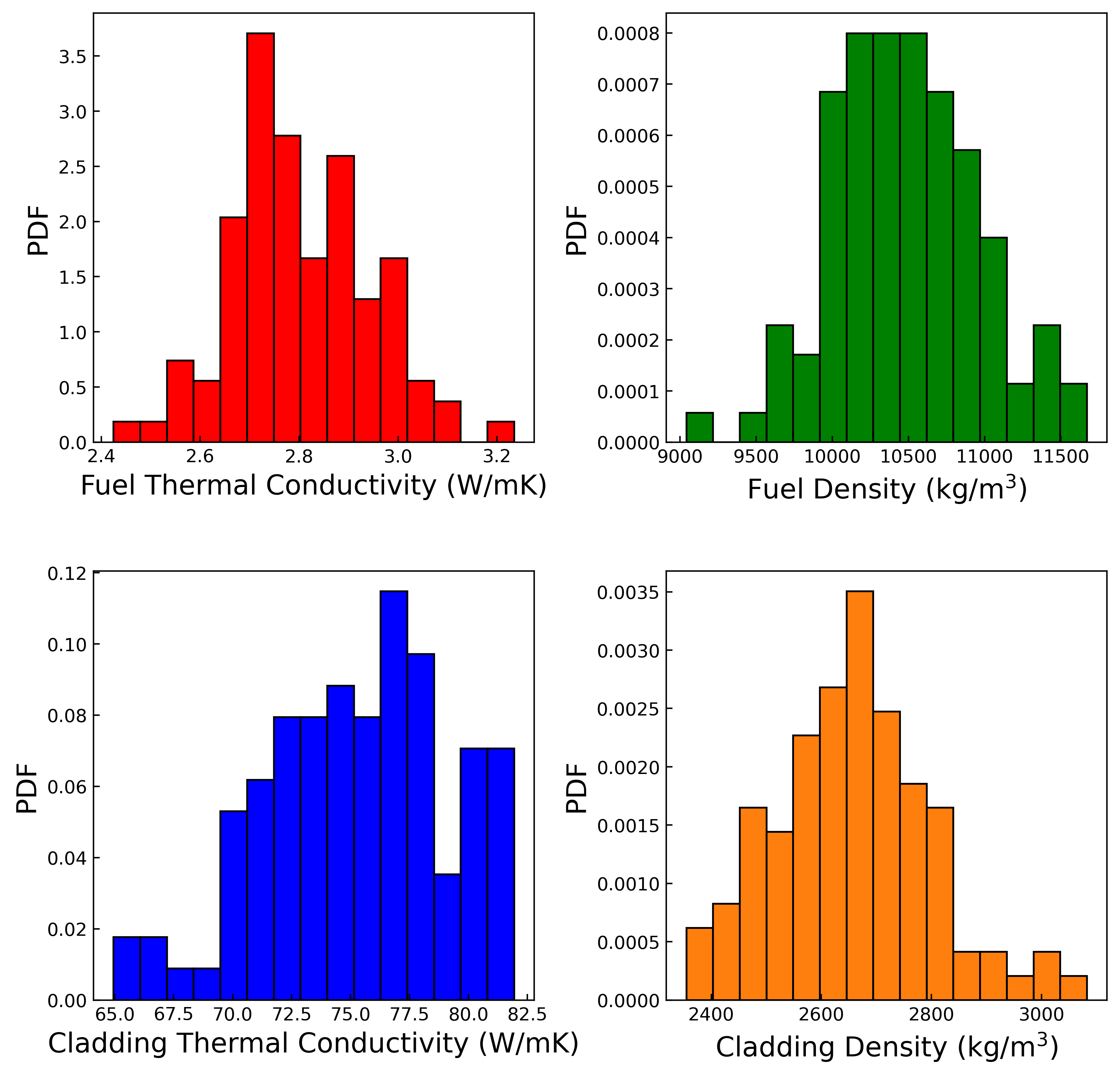
The outputs were maximum cladding surface temperatures, maximum fuel centerline temperatures, and fission gas production in the fuel. The time from before the reactor operation to one year later was divided into 29 steps, and the outputs at each step were obtained. For example, Fig. 3 represents the PDFs at 176.8 days after the reactor operation started.

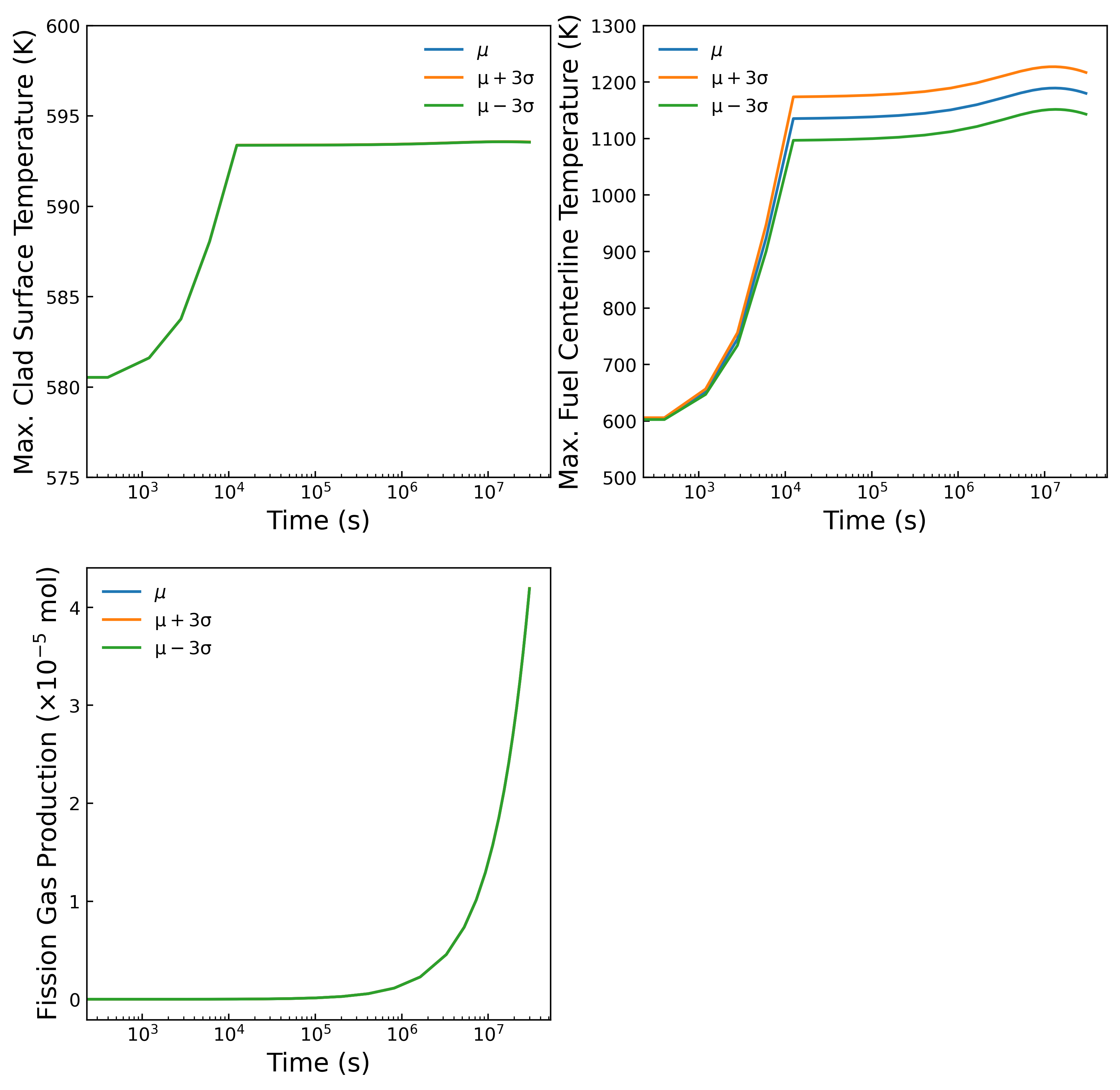
The time evolution of the PDFs produced from the PCE procedure is shown in Fig. 4. The x-axis corresponds to the reactor operation time in seconds and the y-axis the output value. It was provided by solving Eq. 11. The means and the variances for each output value were introduced by Eq. 3 and 4, respectively. The blue solid line shows the mean values, and the orange and green ones represent variances ( $3\sigma$ ). It was observed that the maximum cladding surface and fuel centerline temperatures are proportional to the reactor operation time by $\sim 10^{4}$ seconds, and then keep an almost flat value with slight fluctuations. In contrast, the fission gas production is prolonged and starts a quick increment after $\sim 10^{6}$ seconds. For the maximum cladding surface temperatures and fission gas productions, it can be seen that the uncertainties due to the input variables are not critical. However, these results show the case with a relatively small amount of uncertainty. Therefore, when the uncertainty of input is expected to be greater than that value, the UQ calculation must be performed again for new input parameters.

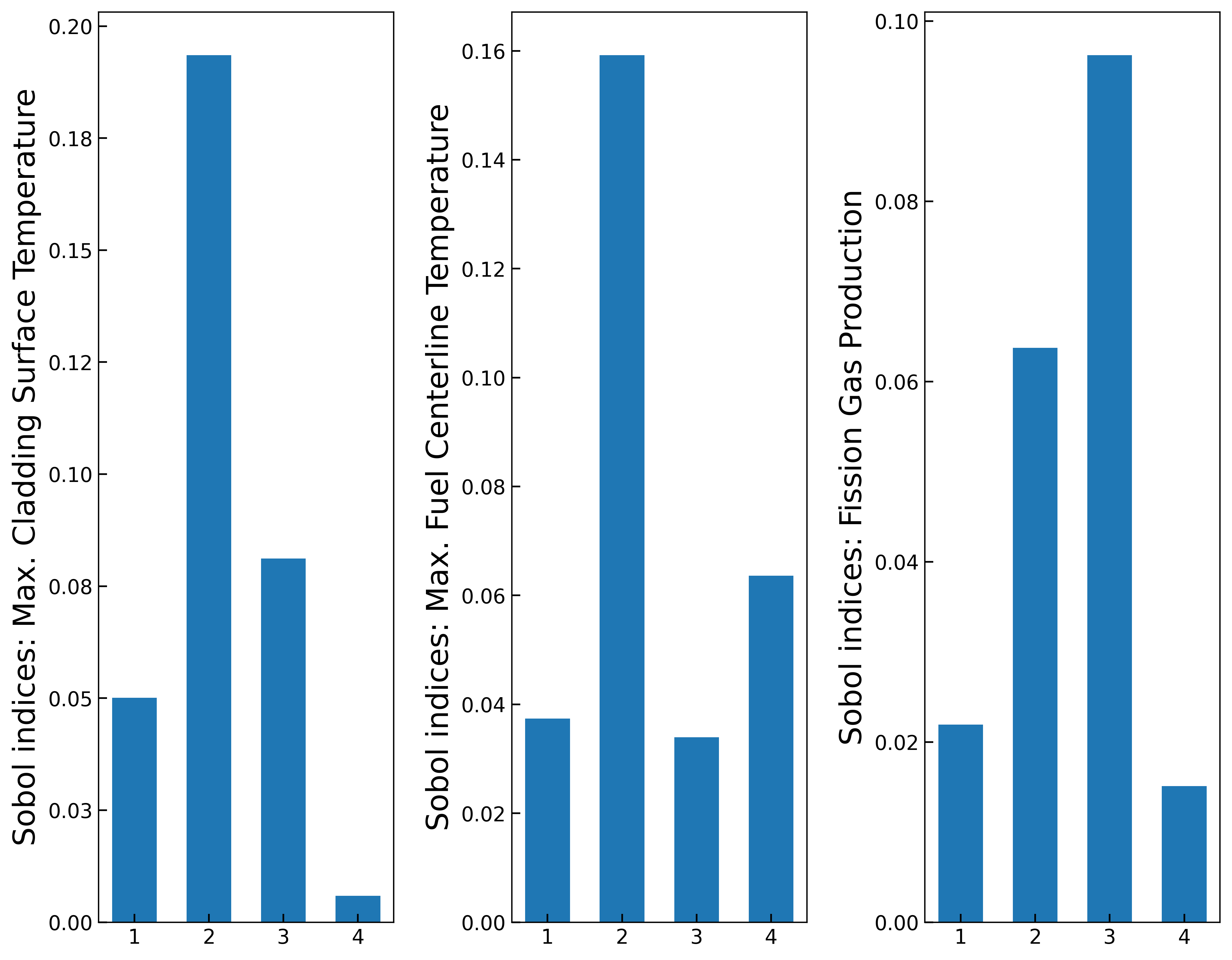
The sensitivity analysis was performed with the results of uncertainty quantification. The impact of uncertain inputs on output responses was quantified and the results are shown in Fig. 5. The x-axis shows the input variable name, 1: fuel thermal conductivity, 2: fuel density, 3: cladding thermal conductivity, and 4: cladding density. The y-axis shows the Sobol indices of the outputs with respect to the input uncertainties. The analysis reveals the relationships between input variables and output responses:

•

Cladding surface temperature: the largest contribution comes from the fuel density and the smallest one from the cladding density
•

Fuel centerline temperature: the largest contribution comes from the fuel density and the smallest one from the cladding thermal conductivity
•

Fission gas production: both the fuel density and cladding thermal conductivity have large contributions, and the smallest contribution comes from the cladding density

Conclusion

The use of digital twin technology is a top priority for future nuclear power development, data analysis and modeling methods that apply artificial intelligence and machine learning are expected to develop further in the future. Among Machine learning-based data-driven methods, uncertainty quantification and sensitivity analysis are necessary in terms of designing complex systems such as nuclear reactors. However, their applications in nuclear power systems are very limited right now. The demonstration was performed with one of the next-generation nuclear fuel performance codes to introduce these methods to the nuclear field: BISON. As a result, the impact of uncertain inputs and their contribution to the output values were quantified. An advantage of these methods is to treat a simulator as a black box. In other words, the user can implement these methods into any other nuclear codes: for example, neutronics, CFD, fuel performance, and even their coupling simulations. This advantage will significantly benefit the evaluation of new materials for advanced reactor systems (e.g. accident tolerant fuels, high-temperature gas reactors, and fusion reactors), with significant uncertainties due to a lack of experimental data. In another application, it is possible to evaluate the impact of each reactor design parameter on the entire system and quantify the impact on the operation. In conclusion, uncertainty quantification and sensitivity analysis may contribute to the nuclear field: by accelerating R&D and enhancing risk assessment.

Acknowledgement

The computational part of this work was supported in part by the National Science Foundation (NSF) under Grant No. OAC-1919789.

References

Kobayashi and Alam [2022] Kazuma Kobayashi and Syed Alam. Practical applications of gaussian process with uncertainty quantification and sensitivity analysis for digital twin for advanced nuclear fuel. In Springer Handbook of Smart Energy System (Accepted in press). Springer Nature, 2022.
Kobayashi et al. [2022] K. Kobayashi, B. Bloss, Alexander F, B. Kelly, A. Alajo, D. Kumar, and S Alam. Digital twin for multi-criteria decision-making framework to accelerate fuel qualification for accident tolerant fuel concepts. In Springer Handbook of Smart Energy System (Accepted in press). Springer Nature, 2022.
Rahman et al. [2022] M Rahman, A H Khan, D Kumar, Kazuma Kobayashi, and Syed Alam. Leveraging industry 4.0 - deep learning, surrogate model and transfer learning with uncertainty quantification incorporated into digital twin for nuclear system. In Springer Handbook of Smart Energy System (Accepted in press). Springer Nature, 2022.
Carmack et al. [2013] Jon Carmack, Frank Goldner, Shannon M. Bragg-Sitton, and Lance L. Snead. Overview of the u.s. doe accident tolerant fuel development program. 9 2013. URL https://www.osti.gov/biblio/1130553.
Singh et al. [2018a] G Singh, R Sweet, NR Brown, BD Wirth, Y Katoh, and K Terrani. Parametric evaluation of sic/sic composite cladding with uo2 fuel for lwr applications: fuel rod interactions and impact of nonuniform power profile in fuel rod. Journal of Nuclear Materials, 499:155–167, 2018a.
Singh et al. [2018b] Gyanender Singh, Kurt Terrani, and Yutai Katoh. Thermo-mechanical assessment of full sic/sic composite cladding for lwr applications with sensitivity analysis. Journal of Nuclear Materials, 499:126–143, 2018b.
Kumar et al. [2020a] Dinesh Kumar, Yao Koutsawa, Gaston Rauchs, Mariapia Marchi, Carlos Kavka, and Salim Belouettar. Efficient uncertainty quantification and management in the early stage design of composite applications. Composite Structures, 251, nov 2020a. ISSN 02638223. doi:10.1016/j.compstruct.2020.112538.
Kumar et al. [2021] Dinesh Kumar, Syed Alam, Tuhfatur Ridwan, and Cameron S. Goodwin. Quantitative risk assessment of a high power density small modular reactor (SMR) core using uncertainty and sensitivity analyses. Energy, 227:120400, 2021. ISSN 03605442. doi:10.1016/j.energy.2021.120400. URL https://doi.org/10.1016/j.energy.2021.120400.
[9] Idaho National Laboratory. Bison: A finite element-based nuclear fuel performance code. URL https://bison.inl.gov/SitePages/Home.aspx.
Kumar et al. [2016] Dinesh Kumar, Mehrdad Raisee, and Chris Lacor. An efficient non-intrusive reduced basis model for high dimensional stochastic problems in cfd. Computers and Fluids, 138:67–82, 2016. ISSN 00457930. doi:10.1016/j.compfluid.2016.08.015. URL http://dx.doi.org/10.1016/j.compfluid.2016.08.015.
Kumar et al. [2020b] D. Kumar, S. B. Alam, Dean Vučinić, and C. Lacor. Uncertainty quantification and robust optimization in engineering. Lecture Notes in Mechanical Engineering, pages 63–93, 2020b. ISSN 21954364. doi:10.1007/978-981-13-9806-3_3/FIGURES/14. URL https://link.springer.com/chapter/10.1007/978-981-13-9806-3_3.
Walters [2003] Robert Walters. Stochastic fluid mechanics via polynomial chaos. American Institute of Aeronautics and Astronautics, 1 2003. ISBN 978-1-62410-099-4. doi:10.2514/6.2003-413. URL https://arc.aiaa.org/doi/10.2514/6.2003-413.
Sobol [2001] Ilya M Sobol. Global sensitivity indices for nonlinear mathematical models and their monte carlo estimates. Mathematics and computers in simulation, 55(1-3):271–280, 2001.
Cardinal and Aitken [2013] Rudolf N Cardinal and Michael RF Aitken. ANOVA for the behavioral sciences researcher. Psychology Press, 2013.
Wu and Yin [2022] Xuezhi Wu and Bangyue Yin. Mechanism and properties of uo2–graphene composite fuel prepared by in situ synthesis. Crystals, 12(2):230, 2022.
Kowbel et al. [2000] W Kowbel, C A Bruce, K L Tsou, K Patel, J C Withers, and G E Youngblood. High thermal conductivity SiC/SiC composites for fusion applications. Journal of Nuclear Materials, 283-287:570–573, 2000. ISSN 0022-3115. doi:https://doi.org/10.1016/S0022-3115(00)00213-0. URL https://www.sciencedirect.com/science/article/pii/S0022311500002130.