Risk-Awareness in Learning Neural Controllers for Temporal Logic Objectives
Abstract
In this paper, we consider the problem of synthesizing a controller in the presence of uncertainty such that the resulting closed-loop system satisfies certain hard constraints while optimizing certain (soft) performance objectives. We assume that the hard constraints encoding safety or mission-critical task objectives are expressed using Signal Temporal Logic (STL), while performance is quantified using standard cost functions on system trajectories. In order to prioritize the satisfaction of the hard STL constraints, we utilize the framework of control barrier functions (CBFs) and algorithmically obtain CBFs for STL objectives. We assume that the controllers are modeled using neural networks (NNs) and provide an optimization algorithm to learn the optimal parameters for the NN controller that optimize the performance at a user-specified robustness margin for the safety specifications. We use the formalism of risk measures to evaluate the risk incurred by the trade-off between robustness margin of the system and its performance. We demonstrate the efficacy of our approach on well-known difficult examples for nonlinear control such as a quad-rotor and a unicycle, where the mission objectives for each system include hard timing constraints and safety objectives.
I Introduction
Safety-critical cyber-physical systems typically have hard safety specifications that must be met by all system behaviors to guarantee system safety. Additionally, due to efficiency concerns, system designers often specify performance objectives, and seek controllers to optimize these objectives. For example, consider an autonomous vehicle (AV) following another vehicle. Here, the AV must satisfy the safety specification of maintaining a minimum safe distance () from the lead vehicle. However, the system designer may also want to minimize the travel time for the AV. Clearly, the vehicle can be safe with a high robustness margin by driving slower than required (maintaining distance much greater than ), but this leads to sub-optimal performance w.r.t. the travel time objective. In many cases, designing for safety and performance objectives may require design trade-offs. While designers must never violate safety requirements in favor of performance, they can trade-off the safety margin against performance. This trade-off thus generates some risk: from a safety perspective how risky is to use a controller that may perform better with a lower safety margin? In this paper, we systematically study this problem.
We assume that safety specifications are provided in a real-time temporal logic such as Signal Temporal Logic (STL) [1]. STL has recently emerged as a powerful specification language in the various cyber-physical system applications [2, 3, 4, 5]. In STL properties, predicates over real-valued signals form atomic subformulae which can be combined using Boolean logic connectives (such as and, or, not), and temporal logic operators (such as eventually, always, until) that are indexed by time intervals. For example consider a design objective for a quadcopter: “The quadcopter must rendezvous in one of two designated regions or exactly 5 to 7 minutes after takeoff before getting as close as possible to a given target destination within 20 mins, while avoiding no-fly zones.” Let denote the position of the quadcopter. The hard safety specifications in this objective can be expressed by the following STL formula:
| (1) |
The soft specification requires us to minimize , where is a distance function and is the target. An advantage of STL is that we can quantify how robustly a given system behavior satisfies an STL property using the notion of a robustness value [6]. Given a system behavior and a specification, the robustness can be thought of as a signed distance from the given system behavior to the set of behaviors satisfying the property. We can say that a system has safety robustness margin if the minimum robustness value across all its system behaviors exceeds . We assume that a performance objective is specified as any differentiable, real-valued function of the system behavior.
There has been considerable amount of research on the problem of synthesizing controllers that guarantee STL specifications. For example, using approaches from motion planning [7, 8], model predictive control [3, 9, 10], reactive synthesis [11, 12], reinforcement learning [13, 14], imitation learning [15, 16], and through the use of control barrier functions [17, 18]. Of these approaches, the most relevant to our paper is the one based on using control barrier functions (CBFs) [19]. A CBF describes a set such that for all system states , there exists a control action that ensures that . Control synthesis from CBFs has seen a lot of recent work [20, 21, 19]. Recent work has focused on CBFs that provide more general classes of invariants such as timed reachability [22, 23] and fragments of STL [24]. Prima facie, synthesis of controllers to satisfy STL specifications may look like a well-studied problem, however, several open problems remain:
- 1.
- 2.
Existing approaches do not consider the trade-off between safety and performance. A naïve encoding of the problem using Lagrange multipliers (as we show in this paper) does not scale, thus demonstrating the need for a more nuanced approach.
- 3.
Many existing approaches focus on control of linear systems or simple nonlinear systems.
- 4.
Existing work does not quantify risk awareness in trading off safety margin versus system performance.
To address all the above challenges, we first formulate an objective function that combines a CBF for STL-based safety specifications with performance objectives using Lagrange multipliers. We then demonstrate that the Lagrangian optimization approach does not scale. We provide an algorithm to automatically generate the CBF for the STL specification directly from its structure. An important consideration in the CBF is our use of the weighted average of subformula CBFs to generate the CBF for a disjunctive formula.
Next, we introduce deep neural network (DNN)-based controllers to handle arbitrary nonlinear systems. We train the DNN-based controllers in a model-free fashion using a stochastic gradient optimization method that uses adaptive moments. Our optimization formulation is similar to the problem of training a recurrent neural network (RNN), where a cascade of NNs for a given temporal horizon is trained. A crucial aspect of our optimization algorithm is to explicitly guide the search for DNN parameters using a robustness margin parameter: across iterations, the optimizer alternates between satisfying safety and performance based on the robustness of the DNN controller vis-à-vis the desired robustness margin.
Finally, we evaluate the risk-awareness for each designed controller by picking different robustness margins as design parameters. For this analysis, we utilize the recently formulated risk-aware verification approach [25] that uses risk measures such as value-at-risk and conditional-value-at-risk. We demonstrate the efficacy of our method on several examples of nonlinear systems and disjunctive STL safety specifications.
II Background
In this section, we provide the mathematical notation and the overall problem definition. We use bold letters to indicate vectors and vector-valued functions, and calligraphic letters to denote sets.
Let and respectively be the variables denoting state and control inputs taking values from compact sets and , respectively. We use the words action and control input interchangeably. We consider discrete-time nonlinear feedback control systems of the following form11 1 Our technique can handle continuous-time nonlinear systems as well. This requires zero-order hold discretization of the dynamics in a sound way to account for system behavior between sample times.:
| (2) |
Here, and denote the values of the state and action variables at time . We assume that the controller can be expressed as a parameterized function , where is a vector of parameters that takes values in . Later in the paper, we instantiate the specific parametric form using a neural network for the controller. Given a fixed vector of parameters , the parametric control policy returns an action as a function of the current state and time . Namely,
| (3) |
We will be using the terms controller and control policy interchangeably. Under a fixed policy, Eq. (2) is an autonomous discrete-time dynamical system. For a given initial state and dynamics , a system trajectory is a function from to , where , and for all , . To address modeling inaccuracies, we also consider bounded uncertainty in the model. We denote as the family of possible realizations of the model . If the policy is obvious from the context, we drop the in the notation . The main objective of this paper is to formulate algorithms to obtain the optimal policy that guarantees the satisfaction of certain task objectives and safety constraints while optimizing performance rewards. In the rest of the section, we formulate controller synthesis as an optimization problem that we seek to solve. In order to define this formally, we first introduce a performance reward, and then introduce task objectives/safety constraints.
Performance reward. In practical control applications, it is common to quantify the control performance using a state-based reward function [26],[27]. Formally,
Definition 1 (Performance reward for a trajectory)
Given a reward function , and discount factor, , the performance reward of a trajectory initiating in state , under policy is defined in Eq. (4).
| (4) |
Task Objectives and Safety Constraints. We assume that task objectives or safety constraints of the system are specified in a temporal logic known as Signal Temporal Logic (STL)[1]. STL formulas are defined using the following syntax:
|
|
(5) |
Here, , is a function from to , and is a closed interval .
Semantics. The formal semantics of STL over discrete-time trajectories have been previously discussed in [6]. We denote the formula being true at time in trajectory by . We say that iff . The semantics of the Boolean operations (, ) follow standard logical semantics of conjunctions and disjunctions respectively. For temporal operators, we say is true if there is a time where is true. Similarly, is true iff is true for all . Finally, if there is a time where is true and for all times is true.
In addition to the Boolean satisfaction semantics, STL also permits quantitative satisfaction semantics. These are defined with a robustness function evaluated over a trajectory. We omit the formal definition; it can be found in [6, 1]. Intuitively, the robustness function defines robustness of predicates at a given time to be proportional to the signed distance of the state variable value at from the set of values satisfying the predicate. Conjunctions and disjunctions map to minima and maxima of the robustness of their subformulas respectively. Temporal operators can be viewed as conjunctions/disjunctions (or their combinations) over time. We denote as the robustness of the trajectory starting in state for the dynamics . Note that if then it implies that .
Risk Measures. We now introduce two commonly used risk measures that are used to provide probabilistic guarantees of system correctness. We assume that we are provided with a probability distribution on model uncertainties (which is a distribution on ), and to denote a distribution over the initial states of the system. A risk measure at a given threshold (denoted ) is a quantity that can be used to provide the following probabilistic guarantee about the robustness of a given STL specification for the system:
| (6) |
We now include two of the standard risk measures used in literature from [28].
Definition 2 (Value-at-Risk (), Conditional-Value-at-Risk () [28])
Let be shorthand for . The Value-at-Risk is defined as follows:
| (7) |
The conditional-value-at-risk is defined as follows:
| (8) |
Essentially, both risk measures provide probabilistic upper bounds on the negative of the robustness value, or provide lower bounds on the actual robustness value, as is required in risk-aware verification [25, 28].
Problem Definition. (i) Learn an optimal policy such that it satisfies a given STL formula while maximizing the performance reward defined in Eq. (4).
| (9) |
(ii) Given a confidence threshold , we will compute the risk measure that guarantees that: .
III Control Barrier Functions for STL
In [17], the authors introduce time-varying control barrier functions that are used to synthesize controllers that are guaranteed to satisfy a given STL specification. We first adapt this notion to discrete-time nonlinear systems.
Definition 3 (Discrete-Time Time-Varying Valid Control Barrier Functions (DT-CBF))
Let be a
function that maps a state and a time instant to a real value. Let
be a time-varying set. The
function is a valid, discrete-time, time-varying CBF if it
satisfies the following condition:
The zero levelsets of the CBF are an envelope for any system trajectory, i.e.,
| (10) |
|
|
DT-CBF for STL. We formulate CBFs in a recursive fashion based on the formula structure. We describe the overall procedure in Algorithm 1. Before we describe the actual algorithm, we introduce some helper functions. The function defined in Eq. (11) has been used in the past by several approaches [16, 29, 30] as a smooth approximation for computing the minimum of a number of real-valued quantities. In our function, we introduce an additional parameter that is used to control the level of conservatism in the approximation. Intuitively, as larger values of reduce the conservatism but require greater numeric precision. Later, we discuss how the function appears as a part of a cost function to be optimized; we include as a part of this optimization process.
| (11) |
We also define the weighted average function . We are interested in two different form of presented in Eq. (12) and Eq. (13); here .
| (12) |
| (13) |
where the former is more accurate but the latter is more efficient for gradient descent. Finally, we articulate useful properties of and in Lemma III.1.
Lemma III.1
For all , and for , the following are true:
| (14) | |||
| (15) |
We can now describe Algorithm 1. The function computes the CBF w.r.t. either an atomic signal predicate or a conjunction of atomic predicates. The CBF for an atomic predicate of the form is defined using a function that ensures that is positive if is positive, if it is zero and negative otherwise. The CBF of the conjunction of two predicates is simply the of the CBFs of the conjuncts. In the function , we consider four cases. If is a formula of the form , then we return the of for all . If is of the form , then we return the weighted average of the CBFs at all time instants in . For conjunctions of either kinds of temporal formulas, we again return the and for disjunctions, we return the weighted average. Note that the function can be invoked with a concrete trajectory whereupon it returns a numeric value. It can also be invoked with a symbolic trajectory (where the symbols indicate the symbolic state at time ), whereupon it returns a symbolic candidate CBF that is the smooth robustness of the trajectory and is a guaranteed lower bound for trajectory robustness .
Lemma III.2
For any formula belonging to STL, for a given trajectory , if , then .
Proof:
We can prove this recursively over the formula structure and from the identities in Lemma (III.1). It is necessary to mention if it does not imply the STL specifications are violated. ∎
IV Learning-based Control Synthesis
We remark that the trajectory is essentially a repeated composition of and the neural controller. Thus, we can compute the gradient of the performance costs and STL objectives (as expressed by the CBF) with respect to the controller parameters using standard backpropagation methods for neural networks.
IV-A Training Neural Networks to satisfy specifications
We explain the procedure for training a neural controller w.r.t. performance and safety specifications in algorithm 2. The training algorithm aims to approximate the solution of Eq. (9). Thus, the first step is to reformulate it free from constraints. Algorithm 1 provides the smooth trajectory robustness for a given STL formula . This robustness is a function of the common variable that is used by all functions, and the tuple of variables for each subformula of a disjunctive formula (denoted ). In addition to the neural network parameters , we also treat the variables and the sets as decision variables in the training process. The variables are already unconstrained; however, is constrained: . To remove this constraint, we introduce , and use as a decision variable. We denote the tuple of conjunctive variable () and all disjunctive variables () with . We also denote this robustness with that is a function of tuple ,
| (17) |
We also sample a batch of initial states uniformly from for training purposes.
The training algorithm is primarily inspired by the Lagrange multiplier technique that transforms a constrained optimization to non-constrained,
| (18) |
First order optimality conditions guarantee that as long as the Lagrange multipliers are positive, the cost as defined using is positive. This in turn guarantees the satisfaction of STL specifications along the trajectory. Since is highly non-convex, optimization (18) is quite intractable and the solution may not satisfy the KKT optimality condition [31]. However, the main role of the Lagrange multipliers is to perform a trade-off between and and one of the contributions of this work is to propose a training process that focuses on applying this trade off. The training algorithm utilizes the gradients and (obtainable from Automatic differentiation package [32]). In case, the cost specified with is less than a user-specified threshold, then the algorithm increases this with a wise selection between and . Otherwise, it increases the performance with . We call the mentioned user specified threshold as robustness margin (denoted by ).
We now describe Algorithm 2. We use the variable to denote the iteration number during training. We use the notation to denote the value of and at the beginning of iteration . We initialize randomly.
At the beginning of each training iteration, in line 2 we sample from , then in lines (2-2), for all states in , we calculate the gradients , (stored in ), and (stored in ). Of these, note that is . We then compute the state b1 (resp. b2) for which the -norm of (resp. ) is the highest. The gradient values of the states b1 and b2 are respectively stored in and (Line 2).
The next step is to compute potential updates to the parameter values and the STL parameters (Lines 2-2). Roughly, the values represent the update to using only the inclusion of gradient for performance cost in Adam optimizer. The values represent the update only using the gradient of smooth trajectory robustness in Adam optimizer. Finally, represents a slower update with gradient of performance for some .
Next, we sample a state uniformly at random and use it for cost computation. If , i.e., our user-provided robustness margin (Line 2), then we need to take steps to increase the smooth trajectory robustness. We consider two cases: (1) If using the update based on the gradient of the performance cost improves the smooth trajectory robustness, we choose this update as it allows us to improve both performance and robustness, i.e., satisfaction robustness (Line 2). (2) Otherwise, we use the update based on the gradient of the smooth trajectory robustness (Line 2).
If , then we are robustly satisfying our STL constraints. In further quest to improve the performance cost, we need to take care that we do not reduce the robustness margin w.r.t. STL constraints. Hence, we use a slower learning rate that takes smaller steps in trying to improve the performance (Line 2).
Remark 1
Considering that this algorithm only focuses on increasing up to , once the STL specification is satisfied then it focuses on optimizing performance. In a sense, this switching strategy plays a role similar to that of Lagrange multipliers: performance cost is optimized only if the robustness is above the user-provided threshold.
IV-B Risk estimation
The minimum number of samples to guarantee the confidence on the verification results is proposed in [33]. We generate samples uniformly from and simulate the corresponding trajectories . We compute the robustness for every single trajectory and calculate through obtaining the percentile of the negation of the robustness values [34] and calculate according to definition 8.
V Experimental Evaluation
V-A Unicycle Dynamics
We demonstrate the efficacy of our technique on a nonlinear unicycle model. We define the uncertainty for the initial condition as:
|
|
The unicycle dynamics with uncertainties are defined as follows,
| (19) |
where and the control inputs, are bounded: , . To restrict the controller in proposed bounds we fix the last hidden layer of neural controller and include it to model. Thus, we reformulate the dynamics by replacing the controllers with:


| Example | Training | Validation | ||||||
| Controller | Activation | Iterations | Runtime | Expected value | Expected value | |||
| Dimension | Function | (secs) | Performance | / | ||||
| Unicycle | 0.3 | 1e2 | [4,5,2,2] | tanh | 40000 | 1048 | 35.3430 | 0.6108 / 0.6109 |
| Unicycle | 0.5 | 1e2 | [4,5,2,2] | tanh | 40000 | 1067 | 33.3528 | 0.8456 / 0.8518 |
| Quadrotor | 0.1 | 5e4 | [7,10,3,3] | tanh | 10000 | 155 | 24.3024 | 0.6729 / 0.7516 |
Example CBF for atomic propositions, Reward discount Unicycle 0.9 Quadrotor 0.9
Confidence Unicycle Dynamics Quadrotor Dynamics Threshold 0.95 0.246 0.132 0.540 0.417 0.527 0.455 0.98 0.133 0.036 0.421 0.311 0.452 0.395 0.99 0.059 -0.027 0.336 0.239 0.406 0.360 0.999 -0.133 -0.191 0.121 0.067 0.305 0.284


V-B Quadrotor Dynamics
In another attempt we consider controlling a quadrotor with uncertain dynamics. We define the uncertainty for the initial condition as a spherical set, with center, and radius . The quadrotor also follows the following uncertain dynamics,
discretized with ZOH for timestep sec. Here and the control inputs, . The parameter is the gravity. To impose bounds on the controller, like the Unicycle example, we fix the last hidden layer of the neural controller, and include it in the model,
V-C Results
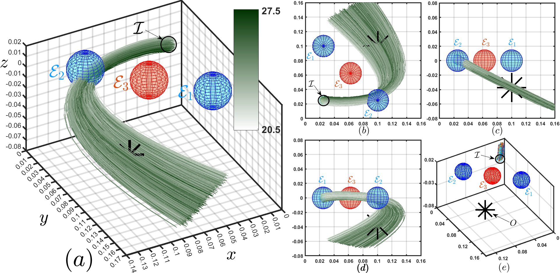
The STL specifications for both examples are adopted from [15] and are introduced in Eq. (16) (Example 1). Regions and for unicycle and quadrotor examples are introduced in Fig 3 and Fig. 4 respectively. The unicycle and quadrotor approaches to the target respectively. They are planned to approach with the highest possible level of performance (fast and close) within time steps. The reward function and CBFs are defined in table II for both examples. We train a controller to satisfy the performance and STL task for unicycle and quadrotor dynamics. Table I shows the training result for in unicycle and in quadrotor example. This table shows the trade-off between performance and STL robustness for the unicycle example.
We utilized (12) and (13) in training the disjunctive parameters for unicycle and quadrotor respectively. Fig. 5 shows the evolution of disjunctive parameters over the training process. Fig. 1 and 2 present the trade-off between the performance cost and trajectory robustness over the training process for both examples. Fig. 3 and Fig. 4 present the simulation of trajectories for unicycle and quadrotor examples, respectively.
Table III presents the results on probabilistic verification or risk-analysis for the controllers. For the unicycle dynamics, we can see that increasing the robustness margin parameter leads to an increase in the (probabilistic) lower bound on the robustness. Increasing the confidence level reduces the probabilistic lower bound. In fact, at 99.9% confidence, there is a risk of seeing system behaviors that violate the specifications by a margin of . Similar risks can be seen at the 99% and 99.9% confidence in the values. Intuitively, table III matches our expectation that controllers designed with higher robustness margin should have lower risk of violating specifications (at the cost of performance).


VI Conclusion and Future work
In this work we propose the weighted average, a useful tool to include disjunctive STL formula in the existent soft constrained policy optimization techniques [17]. We also utilize time dependent feedback policies that facilitates control in presence of STL specifications. This enables us to control the model with smaller neural networks. Non-convex optimizations may be intractable for Lagrange multiplier techniques. We address this problem with proposition of a training algorithm that simulates the trade off between objective and its constraints. We finally utilize this training algorithm for non-convex policy optimization with respect to STL specifications.
In the future, we will focus on improving the scalability of the training process. The proposed recurrent structure for feedback models suffers from vanishing or exploding gradient issue. This results in inefficient training for long trajectories and is due to its resemblance to RNN structures. Thus we plan to include LSTM structure with introduction of hidden states between feedback blocks in the recurrent dynamic structure.
References
- [1] O. Maler and D. Nickovic, “Monitoring temporal properties of continuous signals,” in Proc. of FORMATS, 2004, pp. 152–166.
- [2] Y. V. Pant, H. Abbas, R. A. Quaye, and R. Mangharam, “Fly-by-logic: control of multi-drone fleets with temporal logic objectives,” in Proc. of ICCPS, 2018, pp. 186–197.
- [3] V. Raman, A. Donzé, M. Maasoumy, R. M. Murray, A. Sangiovanni-Vincentelli, and S. A. Seshia, “Model predictive control with signal temporal logic specifications,” in Proc. of CDC. IEEE, 2014, pp. 81–87.
- [4] E. Bartocci, J. V. Deshmukh, A. Donzé, G. E. Fainekos, O. Maler, D. Nickovic, and S. Sankaranarayanan, “Specification-based monitoring of cyber-physical systems: A survey on theory, tools and applications.” Springer, 2017.
- [5] D. Aksaray, A. Jones, Z. Kong, M. Schwager, and C. Belta, “Q-learning for robust satisfaction of signal temporal logic specifications,” in Proc. of CDC. IEEE, 2016, pp. 6565–6570.
- [6] G. Fainekos and G. J. Pappas, “Robustness of temporal logic specifications,” in Formal Approaches to Testing and Runtime Verification, ser. LNCS, vol. 4262. Springer, 2006, pp. 178–192.
- [7] S. Karaman and E. Frazzoli, “Sampling-based algorithms for optimal motion planning,” The international journal of robotics research, vol. 30, no. 7, pp. 846–894, 2011.
- [8] Y. Shoukry, P. Nuzzo, I. Saha, A. L. Sangiovanni-Vincentelli, S. A. Seshia, G. J. Pappas, and P. Tabuada, “Scalable lazy smt-based motion planning,” in Proc. of CDC. IEEE, 2016, pp. 6683–6688.
- [9] S. S. Farahani, V. Raman, and R. M. Murray, “Robust model predictive control for signal temporal logic synthesis,” IFAC-PapersOnLine, vol. 48, no. 27, pp. 323–328, 2015.
- [10] E. A. Gol, M. Lazar, and C. Belta, “Temporal logic model predictive control,” Automatica, vol. 56, pp. 78–85, 2015.
- [11] V. Raman, A. Donzé, D. Sadigh, R. M. Murray, and S. A. Seshia, “Reactive synthesis from signal temporal logic specifications,” in Proc. of HSCC, 2015, pp. 239–248.
- [12] L. Lindemann, G. J. Pappas, and D. V. Dimarogonas, “Reactive and risk-aware control for signal temporal logic,” IEEE Transactions on Automatic Control, 2021.
- [13] L. Berducci, E. A. Aguilar, D. Ničković, and R. Grosu, “Hierarchical potential-based reward shaping from task specifications,” arXiv e-prints, pp. arXiv–2110, 2021.
- [14] X. Li, C.-I. Vasile, and C. Belta, “Reinforcement learning with temporal logic rewards,” in Proc. of IROS. IEEE, 2017, pp. 3834–3839.
- [15] W. Liu, N. Mehdipour, and C. Belta, “Recurrent neural network controllers for signal temporal logic specifications subject to safety constraints,” IEEE Control Systems Letters, vol. 6, pp. 91–96, 2021.
- [16] S. Yaghoubi and G. Fainekos, “Worst-case satisfaction of stl specifications using feedforward neural network controllers: A lagrange multipliers approach,” ACM Transactions on Embedded Computing Systems, vol. 18, no. 5S, 2019.
- [17] L. Lindemann and D. V. Dimarogonas, “Control barrier functions for signal temporal logic tasks,” IEEE control systems letters, vol. 3, no. 1, pp. 96–101, 2018.
- [18] ——, “Robust control for signal temporal logic specifications using discrete average space robustness,” Automatica, vol. 101, pp. 377–387, 2019.
- [19] X. Xu, P. Tabuada, J. W. Grizzle, and A. D. Ames, “Robustness of control barrier functions for safety critical control,” IFAC-PapersOnLine, vol. 48, no. 27, pp. 54–61, 2015.
- [20] A. D. Ames, S. Coogan, M. Egerstedt, G. Notomista, K. Sreenath, and P. Tabuada, “Control barrier functions: Theory and applications,” arXiv preprint arXiv:1903.11199, 2019.
- [21] P. Nilsson and A. D. Ames, “Barrier functions: Bridging the gap between planning from specifications and safety-critical control,” in Proc. of CDC, 2018, pp. 765–772.
- [22] K. Garg, E. Arabi, and D. Panagou, “Prescribed-time convergence with input constraints: A control lyapunov function based approach,” in Proc. of ACC, pp. 962–967.
- [23] K. Garg and D. Panagou, “Control-lyapunov and control-barrier functions based quadratic program for spatio-temporal specifications,” in Proc. of CDC, 2019, pp. 1422–1429.
- [24] L. Lindemann and D. V. Dimarogonas, “Control barrier functions for signal temporal logic tasks,” IEEE Control. Syst. Lett., vol. 3, no. 1, pp. 96–101, 2019. [Online]. Available: https://doi.org/10.1109/LCSYS.2018.2853182
- [25] P. Akella, M. Ahmadi, and A. D. Ames, “A scenario approach to risk-aware safety-critical system verification,” arXiv preprint arXiv:2203.02595, 2022.
- [26] B. D. Anderson and J. B. Moore, Optimal control: linear quadratic methods. Courier Corporation, 2007.
- [27] R. S. Sutton and A. G. Barto, Reinforcement learning: An introduction. MIT press, 2018.
- [28] L. Lindemann, L. Jiang, N. Matni, and G. J. Pappas, “Risk of stochastic systems for temporal logic specifications,” 2022. [Online]. Available: https://arxiv.org/abs/2205.14523
- [29] Y. V. Pant, H. Abbas, and R. Mangharam, “Smooth operator: Control using the smooth robustness of temporal logic,” in Proc. of CCTA. IEEE, 2017, pp. 1235–1240.
- [30] K. Leung, N. Aréchiga, and M. Pavone, “Backpropagation for parametric stl,” in 2019 IEEE Intelligent Vehicles Symposium (IV). IEEE, 2019, pp. 185–192.
- [31] S. Boyd and L. Vandenberghe, “Convex optimization,” 2004.
- [32] A. Paszke, S. Gross, S. Chintala, G. Chanan, E. Yang, Z. DeVito, Z. Lin, A. Desmaison, L. Antiga, and A. Lerer, “Automatic differentiation in pytorch,” 2017.
- [33] M. C. Campi and S. Garatti, “The exact feasibility of randomized solutions of uncertain convex programs,” SIAM Journal on Optimization, vol. 19, no. 3, pp. 1211–1230, 2008.
- [34] R. T. Rockafellar and S. Uryasev, “Optimization of conditional value-at-risk,” Journal of Risk, vol. 2, pp. 21–41, 2000.