Group sequential hypothesis tests with variable group sizes: optimal design and performance evaluation
Andrey Novikov
Metropolitan Autonomous University, Mexico City, Mexico
Abstract:
In this paper, we propose a computer-oriented method of construction of optimal group sequential hypothesis tests with variable group sizes.
In particular, for independent and identically distributed observations we obtain the form of optimal group sequential tests which turn to be a particular case of sequentially planned probability ratio tests [Schmitz 1993, SPPRTs, see].
Formulas are given for computing the numerical characteristics of general SPPRTs, like error probabilities, average sampling cost, etc.
A numerical method of designing the optimal tests and evaluation of the performance characteristics is proposed, and computer algorithms of its implementation are developed.
For a particular case of sampling from a Bernoulli population, the proposed method is implemented in R programming language, the code is available in a public GitHub repository.
The proposed method is compared numerically with other known sampling plans.
Keywords: sequential analysis;
sequentially planned procedure;
hypothesis test;
optimal sampling; optimal stopping
Subject Classifications: 62L10, 62L15, 62F03, 60G40
1. INTRODUCTION
Group sequential hypothesis tests with variable group sizes have been proposed as a theoretical framework for some practical situations when sequential statistical methods are applied to sampling data in groups. In many occasions, the overall cost of sampling in groups includes, additionally to the unitary cost of any collected data item, also some set up cost related to the group, in which case the classical one-per-group sequential plans [Wald and Wolfowitz 1948, see] may not be optimal with respect to the total cost [Cressie and Morgan 1993]. Ehrenfeld 1972 used the general principle of dynamic programming for obtaining the form of optimal group sequential sampling plan in the Bayesian set-up, with arbitrary cost function. Schmitz 1993 proposed a unified approach to sequentially planned statistical procedures based on optimal stopping with respect to a partially ordered “time line”. For the sequentially planned hypothesis tests he proposed a general structure of testing procedures, called sequentially planned probability ratio tests (SPPRTs), where the rule responsible for sampling may vary depending on particular problem settings.
For the problem of testing of two simple hypotheses, Schmegner and Baron 2007 studied a class of SPPRTs under the assumption that the log-likelihood ratio takes its values on a lattice. In this case, they obtained analytical expressions for characteristics of the SPPRTs and, in the particular case of symmetric hypotheses about the success probability in the Bernoulli model, evaluated them for various sampling plans known from the literature, aiming at minimisation of the average cost of observations.
Another large area of applications related to the group sequential testing is related to clinical trials. The variable-group-size plans are called adaptive in this context [Dragalin 2006]. In Eales and Jennison 1992, the dynamic programming principle is used for obtaining optimal adaptive group sequential testing procedures in the normal model.
In this paper, we propose a computer-oriented method of construction of optimal group sequential tests with variable group sizes. The basic idea of the proposed method is to use a grid interpolation scheme in the backward induction equations. We develop a complete set of computer algorithms for their design and performance evaluation. For the case of Bernoulli observations, we implement the algorithms in R programming language [R Core Team 2013] and numerically compare the obtained plans with those of Schmegner and Baron 2007. The relative efficiency of the optimal test with respect to the one-stage plan with the same levels of error probabilities is evaluated.
Another application we consider is with respect to the optimal adaptive group sequential tests for Phase II clinical trials based on binary outcomes. In this example we numerically compare the performance of our optimal plans with those proposed by Fleming 1982.
In Section 2, general results on optimal group sequential tests with variable group sizes are summarized. In Section 3, optimal group sequential tests with variable group sizes for independent and identically distributed observations are characterized (which turn out to be of SPPRT type) and formulas for performance characteristics are obtained. In Section 4, a numerical method of optimal sequential planning and evaluation of performance characteristics is proposed. Numerical examples are presened. Section 5 contains a brief summary of results and conclusions.
2. OPTIMAL SEQUENTIALLY PLANNED TESTS
In this section we adapt the results of Novikov 2008 to the context of group sequential tests with variable group sizes. Following Schmitz 1993, we prefer the term “sequentially planned test” to “group sequential test with variable group sizes”.
2.1. Definitions and preliminaries
We assume that a sequence of random variables will be available on the group-by-group basis for testing two simple hypotheses and about their distribution.
A group sequential test is based on a family of rules governing the process of sampling. Let us suppose the process of testing came to stage meaning that groups of observations have been taken, and let be the consecutive sizes of the groups taken. Let the individual observations collected up to stage be . Then the size of the next group to be taken at stage should be defined as a function taking values in a set , where is finite. A positive value of is interpreted as the size of the group of observations to be taken at stage . If , this means no more observations will be taken (and the process should be stopped with the data observed in groups). The size of the first group is defined before any observation is taken and will be denoted as . In this way, a sampling plan is defined as the set of functions .
After the sampling process is stopped, the final decision is taken using another element of the group sequential test called decision function and denoted as . Any takes one of the values 0 or 1, meaning accepting the respective hypothesis or . All the functions and are assumed to be measurable for all and all .
Let us denote the sequentially planned test with the sampling rule and the decision rule .
A classical sequential test corresponds to or 0 (one observation at a time is taken, if any) for all , .
Let us define and, recurrently over ,
Let us define the following events: (stop at stage ), and (stop at or after stage ).
Suppose there is some cost, say , we should pay for any group of items to be observed (for obvious reasons, we can assume that for all ; another natural assumption is that is a strictly increasing function of ). Then the average sampling cost (ASC), under , of carrying out a test based on sampling plan is
where Ej is the symbol of the mathematical expectation calculated under hypothesis , .
Error probabilities of the first and the second kind are defined, respectively, as
The usual context for hypothesis testing is to minimise the average experimental cost under the restriction that
| (2.1) |
where and some numbers between 0 and 1.
In this paper, we want to minimise a weighted average sampling cost
| (2.2) |
under condition (2.1), where is a given fixed number. The value of represents the grade of importance we attribute to ASC1 in comparison with ASC0 when designing the optimal test. The extreme values 0 or 1 correspond to minimisation of ASC under and , respectively, regardless of the value the average cost may have under the other hypothesis. It is most desirable that one test satisfying (2.1) minimise both average sampling costs [Wald and Wolfowitz 1948, just like the classical SPRT in the one-per-group case does, see]. Unfortunately, there is no known result in the literature that could guarantee this property (which may be called Wald-Wolfowitz optimality) for the sequentially planned tests. Anyway, if a test with error probabilities and could ever be found that minimises both and among all the tests subject to (2.1), it should also minimise ASCγ, whatever .
It is easy to see that the problem of minimisation of (2.2) under restrictions (2.1) reduces to the problem of minimisation of
| (2.3) |
with some non-negative [see Novikov 2008, Section 2]. Essentially, this is a straightforward application of the Lagrange method to a problem of constrained minimisation. From this point of view, (2.3) is interpreted as a Lagrangian function with constant multipliers . The multipliers should be used to guarantee that for the test minimising (2.3) equalities in (2.1) are attained.
On the other hand, if then (2.3) can be seen as Bayesian risk [Ehrenfeld 1972, cf. (2.1) in ] in the Bayes formulation. In this case can be interpreted as an a priori probability of hypothesis , and as some characteristics related to the loss due to incorrect decisions.
In a very usual way, it can be shown that there is a unique form for the decision function to be used in (2.3) for its minimisation.
We need some additional notation for this. Let be the Radon-Nikodym density of the distribution of under , , with respect to a product-measure ( times by itself), and let .
For any set of group sizes let us denote where , Let us also define as the product-measure .
Then for any given sampling plan , (2.3) is minimised by the decision function defined as
| (2.4) |
for any ,
The corresponding minimum value of (2.3) is
where . The proof is along the lines of the proof of Theorem 3.1 in Novikov 2008.
2.2. Optimal truncated plans
Let be the set of sampling plans taking at most groups (such that ). For , let us denote
Starting from
define recursively for
Then for any sampling plan
| (2.5) |
There is an equality in (2.5) if a sampling plan is such that for
and .
It follows from (2.5) that this is an optimal sampling plan minimizing in .
This result can be obtained in essentially the same way as Corollary 4.4 in Novikov 2008.
2.3. Optimal non-truncated plans
The treatment of the general case is essentially the same as in Section 5 in Novikov 2008.
First, it can easily be shown that for any fixed , so there exists
Furthermore, as for all .
Therefore, it follows from (2.5) that for all
| (2.6) |
And similarly to the proof of Theorem 5.5 in Novikov 2008 it is shown that there is an equality in (2.6) if a sampling plan is such that for
| (2.7) |
and .
Therefore, this is a form of a sampling plan which minimises the Lagrangian function , over all . All other optimal sampling plans can be obtained from this one by randomisation, similarly to Novikov 2008. The randomisation can be applied in any case of equality between the respective elements in (2.7), including those participating in the argmin definition. Obviously, the randomisation is irrelevant for the Bayesian set-up but may be useful in the conditional setting.
3. THE I.I.D. CASE
In the case of independent and identically distributed (i.i.d.) observations the constructions of Section 2 acquire a much simpler form.
Let be the Radon-Nikodym derivative (with respect to ) of the distribution of under hypothesis , and assume are all independent, . Very naturally, it should be assumed that the hypothesized distributions are distinct: .
3.1. Optimal sequentially planned tests
Let us define operator , defined for any bounded measurable non-negative function , as
Let us denote for .
Starting from
| (3.1) |
define recursively over
| (3.2) |
It is easy to see, by induction, that
where is the likelihood ratio.
Furthermore, the optimal sampling rule depends on , , whatever be and , and , where for and
| (3.3) |
and .
In particular, we obtain here a characterisation of truncated Bayesian sequentially planned test (properly saying, of its sampling-plan part, but the decision function to apply with any sampling plan is universal and is defined in (2.4), so we obtain a complete sequentially planned test which is Bayes-optimal). In fact, (2.4) can also be expressed in terms of the likelihood ratio:
| (3.4) |
for any ,
In the same way, to obtain optimal truncated sequentially planned tests in the conditional set-up we only need to satisfy (2.1) choosing appropriate Lagrangian multipliers and .
At last, a concluding remark on the form of continuation regions of optimal truncated tests. Using the concavity of functions , and other involved, it is not difficult to see that the “continuation region” (see the first line of (3.3)) always has a form of an interval (if not empty). We used this technique in Novikov and Popoca Jiménez 2022 for a related problem, when the group sizes are independent of the observations. In addition, it can be shown that and , where is the last non-empty continuation interval.
The optimal non-truncated tests are obtained by passing to the limit as . It is easy to see that for all (see (3.2)). So there exists , . It is a concave non-decreasing function with .
Passing to the limit in (3.2) as , we obtain
Now, passing to the limit in (3.3), as we see that the optimal sampling plan depends on , in such a way that , for any and and , where for any
| (3.5) |
Once again, the continuation region is an interval with some (if not empty).
The resulting sequentially planned test is a particular case of Secuentially Planned Probability Ratio Tests (SPPRTs) [Schmitz 1993, see (3.5) in ], with , .
In fact, the formal definition of SPPRT in Schmitz 1993 requires that . Our construction (3.5) may result in , but it is still optimal in the class of sequentially planned tests we consider (those taking at least one group of observations).
3.2. Performance characteristics
In this part, we obtain formulas for calculating error probabilities, average sampling cost and some related probabilities, for truncated sequentially planned tests.
Let be a sampling rule depending on , in such a way that , whatever be and , and , and let be any decision rule such that for all and .
Let us denote the event meaning “H0 is accepted at stage or thereafter” (in accordance with the rules of the test ).
Proposition 3.1.
Let
| (3.6) |
and, recursively over ,
| (3.7) |
Then for any
| (3.8) |
in particular,
| (3.9) |
Remark 3.1.
The distribution for use in Proposition 3.1 (in (3.7), (3.8) and (3.9)) is primarily ment to be the one hypothesized under or , but in principle it may be any particular distribution preserving the i.i.d. structure of the observations .
As a particular case, for
so the error probabilities can be calculated using and , respectively, in the evaluation of in Proposition 3.1.
In the same way, the operating caracteristic of the truncated SPPRT in this case can be calculated just using any third distribution of in Proposition 3.1.
Proof of Proposition 3.1. By induction over .
For , it follows from (3.6) that (this latter equality follows from the definition of the decision function).
Let us suppose now that (3.8) holds for some .
Then
Analogously, the average sampling cost can be evaluated as follows.
Proposition 3.2.
Let
and, recursively over ,
| (3.10) |
Then for all
| (3.11) |
In particular,
| (3.12) |
Remark 3.2.
Proof of Proposition 3.2.
By definition,
Let us suppose now that (3.11) is satisfied for some . Then, by definition,
and
which proves (3.11) also for .
Remark 3.3.
For non-truncated SPPRTs , we can also make use of Propositions 3.1 and 3.2, by truncating the sampling plan .
Let us define, for any , as the sampling plan redefined it in such a way that for all (keeping intact all other components of ).
Using the fact that , as , for , we obtain from (3.14) a numerical approximation for .
Also and , so we obtain from Proposition 3.1 a numerical approximation for the error probabilities and .
Remark 3.4.
Proposition 3.2 can also be used for calculating other sampling characteristics of the test.
For example, taking in Proposition 3.2 , for all , one obtains, in place of the ASC, the average number of groups taken, E.
Employing , for all , provides the average number of observations taken,
4. NUMERICAL ALGORITHMS
In this section we propose numerical algorithms for optimal design of sequentially planned tests and their performance evaluation.
4.1. Optimal design and performance evaluation
We propose a numerical method based on the optimal sampling plan described in (3.3).
The sampling plan is entirely based on the sequence of functions defined in (3.1) and (3.2) for . The idea of the method is a numerical approximation of every on the continuation interval by a picewise-linear function based on a grid of -values. So instead of functions we will work with functions defined as follows: let , and define recursively for
where is calculated by interpolation between the grid points on the continuation interval.
Formally, the proposed algorithm is as follows (applicable for ). Numerical implementation of the optimal design (NIOD algorithm)
- Step 1
-
Start from
- Step 2
-
Find a minimum () and a maximum () value of for which
(4.1) If no such exist, declare Early Exit condition and Stop.
- Step 3
-
For a grid of values on calculate and store the respective values of the function on the right in (4.1). Take note, for future use, that will be calculated as for and using an interpolation between the respective grid points for
- Step 4
-
Set . If then Stop, else go to Step 2.
The Early Exit condition means that the optimal testing procedure in fact is truncated at a lower level than , because at step there is no continuation interval, i.e., , . We can incorporate the Early Exit condition into the general scheme simply adjusting the truncation level by taking as the minimum of and . In particular, it may happen that , meaning that only one-stage sampling plans come into question in the hypothesis testing problem with given input parameters (for example, when the cost of data is too high).
In case the algorithm terminates with one stage, the first sample of size is taken, and the decision function (2.4) with is applied.
After the algorithm stops with (corrected for the Early Exit, if applicable), we obtain a way to calculate the functions , , and to apply them in definitions of optimal sampling plans in (3.3) (where and ):
| (4.2) |
and , (let us denote for any and any ).
Respectively, we can use Proposition 3.1 for approximate evaluation of error probabilities by substituting for in (3.7) for :
| (4.3) |
with , and finally from (3.9)
| (4.4) |
as an approximate value of .
Analogously, using E0 instead of E1 in (4.3) for we get an approximation for in the form of
| (4.5) |
In the same way, substituting for (and for ) in Proposition 3.2 we obtain from (3.13) an aproximation for the average sampling cost:
| (4.6) |
whatever the distribution of the i.i.d. observations is used for calculations in Proposition 3.2.
All the computations involve some values of the Lagrange multipliers and that should be determined in such a way that there are equalities in (2.1). In fact, for some and this holds automatically, namely, for and , where is a test minimising (2.3) for some . For other and , there is no way to guarantee the existence of and providing equalities in (2.1), not even in the classical case of purely sequential tests.
To conclude this subsection, let us summarize the algorithm of the optimal test evaluations. The overall procedure is quite straightforward. Optimal test evaluations (OTE algorithm)
- Input parameters:
-
hypothesis points , , Lagrangian multipliers , , grid size , horizon , the set of eligible group sizes , cost function , weight parameter .
- Step 1
-
Run the algorithm NIOD above in this subsection.
- Step 2
-
Calculate the optimal sampling plan (see (3.3)).
- Step 3
- Step 4
-
Calculate the average sampling cost: ASC and ASC, using (4.6).
- Step 5
-
Calculate the Average Number of Observations and/or Average Number of Groups (optional, see Remark 3.4).
- Output:
-
and , ASC and ASC (optionally, the Average Number of Observations and/or the Average Number of Groups).
We implemented this algorithm for the problem of testing hypothesis vs. about the success probability of a Bernoulli distribution. The program code in R programming language [R Core Team 2013] can be downloaded from a public GitHub repository at https://github.com/HOBuKOB-MEX/SPPRT. There is an R function for each step of the above OTE algorithm in the program implementation. The documentation is provided in the repository.
With the program code at hand, it is easy to make the output plan satisfy restrictions (2.1) by varying the input parameters and in a series of trial-and-error iterations. The following empirical fact is very helpful for doing the work. The main effect of is on : larger values make smaller, leaving largely unaffected; similarly, increasing mainly affects making it smaller, with no significant change in .
4.2. Numerical examples
In this subsection, we apply the program code for two practical examples of the optimal sequentially planned tests.
4.2.1. Numerical comparison of sampling plans when testing for majority
Schmegner and Baron 2007 provided a technique for numerical evaluation of the SPPRTs based on general results for random walks, in the particular case when the log-likelihood takes its values on a lattice. The results are applicable, in particular, for testing a hypothesis vs. for the success probability of a Bernoulli distribution. Using the SPPRT with various sampling plans known from the literature (see the details of the plans ibid.), Schmegner and Baron 2007 evaluated the SPPRT for testing vs. in a series of scenarios, searching for the most inexpensive sampling plan in a particular practical context, with respect to the cost function , where (cost per observation) and (cost per group). All the evaluated sampling plans were based on a continuation interval which guaranteed that the error probabilities of the first and second kind were at most . The best value of ASC found was 18254, with an average number of groups of E and an average total number of observations of E [see Schmegner and Baron 2007, Example 4.6].
We present here the results of numerical evaluations corresponding to our optimal test evaluations algorithm in Subsection 4.1, in exactly the same context, to be able to compare the performance of our plan with those in Schmegner and Baron 2007.
For our implementation of the algorithms of Subsection 4.1, we used, in each continuation interval, a uniform grid formed by equidistant points on the logarithmic scale of with step . We used our truncated SPPRT (4.2) with (maximum number of groups to be observed). Also we employed as the set of possible group sizes the set . We used ASCγ with as a criterion of minimisation. The Lagrange multipliers were chosen in such a way that and .
Evaluating the characteristics of the proposed SPPRT according to (4.4) - (4.6) we obtained , with the average number of groups E and the average number of observations E. Thus, our method provides nearly 1.6 times lower sampling cost, in comparison with the best plan found in Schmegner and Baron 2007. Taking into account that there are a number of ways to improve the numerical characteristics, namely, by 1) choosing a higher truncation level , 2) making the grid size smaller, 3) making the set of eligible group sizes “denser”, 4) adjusting the criterion of minimization by varying as required by the practical context, – taking this into account, the real efficiency of the proposed method can turn even higher.
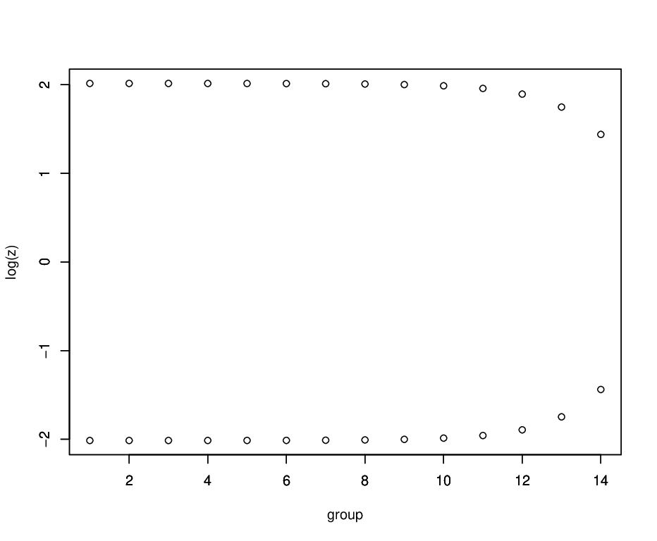
In Figure 1, the set of continuation intervals at each of the fourteen sequentially planned steps is presented. We know that theoretically the continuation interval gets closer to the one corresponding to the optimal non-truncated SPPRT, as . It appears that in this example the convergence is so fast that the interval reaches its limit after as few as some 4 steps (remember that the first interval found comes last).
In Figure 2, one can see the “nearly optimal” sampling plan calculated as a NIOD approxination to (3.5). Again, because converges to the optimal sampling plan as , we may expect that this is approximately the sampling plan the optimal non-truncated SPPRT will use in each step.

Taking into account that the gain from using our method, with respect to other known methods, is comparable to the gain the classical SPRT provides with respect to one-sample (fixed sample size, FSS) test, we would like to examine the efficiency of our method with respect to the one-sample test, in various scenarios. As a reference, we want to use, for given and , the average sampling cost of the one-step test with a minimum sample size that provides error probabilities not exceeding and , respectively. For the Bernoulli model, can be calculated using the NP function from the GitHub repository Novikov et al. 2021.
According to the definition of average sampling cost, the one-sample test has an ASC equal to ASC, which will be compared with ASC of the SPPRT we proposed.
It is interesting to note that for and and used in this example the FSS is equal to , giving the average sampling cost of ASC for the one-sample plan, which outperforms all the SPPRTs examined in Schmegner and Baron 2007.
To compare the performance of our “nearly optimal” SPPRT with that of the one-sample test we ran our program for a series of and between 3 and 6.3 on the scale of natural logarithms, with a total of 9 9 points. For each one, we calculated the corresponding , and ASC0 and ASC1. The relative efficiency was calculated as under hypothesis , .
To get a compact visual representation of the results, we fit a local polynomial regression model (LOESS)11 1 https://www.rdocumentation.org/packages/stats/versions/3.6.2/topics/loess to the data obtained, to represent the relationship between the relative efficiency and and . We use decimal logarithms of and as independent variables, and as response. The result of the model fitting for is shown in Figure 3. The graph of is perfectly symmetric with respect to the diagonal and is not shown.
We see from Figure 3 that the maximum of relative efficiency is attained in the asymmetric case when is small and is relatively large, and is about 2.5. In the vicinity of the diagonal the maximum efficiency of approx. 2.1 is reached for small with a clear tendency of increasing as . The minimum efficiency is about 1.3 and is attained whenever is relatively large.

4.2.2. Adaptive group-sequential test for phase II clinical trials
Sequential hypotheses tests are widely used in clinical trials applications [Jennison and Turnbull 1999, see, for example,]. The most popular are so-called group-sequential methods, when samples of fixed size (groups) are drawn and analysed sequentially (interim analyses), allowing for early termination when sufficient information for acceptance or rejection of the hypotheses is collected. There also exists a class of group-sequential methods called adaptive, when the size of the next group to be taken may depend on the results of interim analyses [Dragalin 2006]. In this way, adaptive group-sequential tests are, in essence, the sequentially planned tests we consider in this paper.
In this subsection, we apply our technique for phase II clinical trials. We refer to the context of Fleming 1982, where a construction of group-sequential sampling plan is proposed for the clinical trials designed for testing therapeutic effect of cancer treatments based on the frequency of tumor “regressions” after the treatment has been applied. It is assumed that the frequencies are binomially distributed with the parameter representing the probability of regressions. The hypotheses of interest are vs. , where . As usual in applications, is considered an indifference zone, and we want to apply our optimal design in Subsection 4.1 to testing a simple hypothesis vs. . We take as a reference the data of Table 12.1 in Jennison and Turnbull 1999.
| Max. 3 groups | Max. 5 groups | |||||||||
| 0.05, 0.2 | 0.1, 0.3 | 0.2, 0.4 | 0.3, 0.5 | 0.3, 0.5 | ||||||
| 0.046 | (0.046) | 0.050 | (0.063) | 0.050 | (0.057) | 0.050 | (0.049) | 0.051 | (0.049) | |
| 0.09 | (0.087) | 0.10 | (0.071) | 0.10 | (0.093) | 0.10 | (0.113) | 0.10 | (0.113) | |
| ASN0 | 34.1 | (31.6) | 23.6 | (24.8) | 30.8 | (30.6) | 36.3 | (31.6) | 36.0 | (31.6) |
| ASN1 | 23.3 | (26.8) | 19.6 | (21.6) | 28.0 | (30.4) | 32.9 | (35.5) | 30.0 | (35.5) |
| ANG0 | 2.2 | 1.8 | 1.7 | 1.8 | 2.3 | |||||
| ANG1 | 1.8 | 1.8 | 1.8 | 1.9 | 2.7 | |||||
| 154 | 126.5 | 199.8 | 229.7 | 230.2 | ||||||
| 57 | 49.2 | 69.8 | 79.1 | 69.1 | ||||||
| 38.4 | 31.8 | 43.4 | 49.9 | 49.7 | ||||||
| 1.13 | 1.34 | 1.41 | 1.37 | 1.38 | ||||||
| 1.65 | 1.62 | 1.55 | 1.52 | 1.66 | ||||||
For each pair of hypothesis points we applied the algorithm OTE of Subsection 4.1 taking as a cost function , with , taking into account that the plans of Fleming 1982 use at most 3 groups. We used for our evaluations the value for the weight coefficient, in order to illustrate the effect of this input parameter on the output performance of the plan. The choice of this parameter can be helpful with the ethical issue of clinical trials: if the treatment is turning out to be not efficient (which corresponds to rejecting ), it should be terminated as soon as possible (meaning the average sample number under should prevail when planning a real clinical trial). Large value of is ment to make the average sample number ASN1 under smaller in comparison with that under , ASN0. We use the grid size of for all the evaluations in this example.
And we use the same nominal and as in Fleming 1982 to be able to compare the performance of the corresponding plans. The multipliers and are used, as intended, to comply with these requirements. A general-purpose gradient-free optimisation method by Nelder and Mead 1965 was used to get as close as possible to the nominal values of and , with respect to the relative distance
| (4.7) |
(the discrete nature of the binomial probabilities does not permit, generally speaking, to make the error probabilities exactly equal to and ).
The fitted results are shown in Table 1. and are the values of the average number of groups the optimal adaptive plan takes under and . The values of and are provided for reproducibility of the results. , exactly as above, is the minimum sample size a one-sample (FSS) test needs to comply with the error probabilities. Respectively, is the relative efficiency the optimal plan exhibits with respect to the non-sequential plan. It is seen that the relative efficiency of the optimal sequentially planned test, with respect to the FSS test is higher than 1.5 in all the cases.
In general, we observe that our optimal adaptive (sequentially planned) tests, with as few as at most three groups allow to save some 2 to 3 analyses (patients) under , on the average, in comparison with the plan of Fleming 1982.
To have an idea of the effect of using more groups, we ran the same fitting procedure using at most groups (last column in Table 1). It obviously is more efficient with respect to the one-sample plan (with the relative efficiency up to 1.66), and saves up to 5 analyses, on the average, in comparison with the 3-group plan.
Our program implementation in https://github.com/HOBuKOB-MEX/SPPRT allows for virtually any number of groups (and any other parameters like , , etc.) when designing optimal plans for the binomial data.
5. CONCLUSIONS
In this paper, we proposed a method of construction of optimal sequentially planned tests. In particular, for i.i.d. observations we obtained the form of optimal sequentially planned tests and formulas for computing their numerical characteristics like error probabilities, average sampling cost, average number of observations and the average number of groups.
A method of numerical evaluation of the performance characteristics is proposed and computer algorithms of their implementation are developed.
For a particular case of sampling from a Bernoulli population, the proposed method is implemented in R programming language providing a computer code in the form of a public GitHub repository.
The proposed method is compared numerically with other known sampling plans.
A numerical comparison of the proposed tests with one-sample tests having the same error probabilities has been carried out. The relative efficiency based on the average sampling cost compared to one-sample tests exhibits largely the same behaviour as that of the classical SPRT does, when the efficiency is based on comparison of the average sample number with the FSS.
ACKNOWLEDGEMENTS
The author gratefully acknowledges a partial support of SNI by CONACyT (Mexico) for this work.
The author thanks the anonymous Reviewers and the Associate Editor for valuable comments and useful suggestions.
References
- Cressie and Morgan [1993] N. Cressie and P. B. Morgan. The VRPT: A sequential testing procedure dominating the SPRT. Econometric Theory, 9:431–450, 1993.
- Dragalin [2006] V. Dragalin. Adaptive designs: Terminology and classification. Drug Information Journal, 40(4):425–435, 2006. doi: 10.1177/216847900604000408. URL https://doi.org/10.1177/216847900604000408.
- Eales and Jennison [1992] J. D. Eales and C. Jennison. An improved method for deriving optimal one-sided group sequential tests. Biometrika, 79(1):13–24, 03 1992. ISSN 0006-3444. doi: 10.1093/biomet/79.1.13. URL https://doi.org/10.1093/biomet/79.1.13.
- Ehrenfeld [1972] S. Ehrenfeld. On group sequential sampling. Technometrics, 14(1):167–174, 1972.
- Fleming [1982] T.R. Fleming. One-sample multiple testing procedure for phase ii clinical trials. Biometrics, 38:143 – 151, 1982.
- Jennison and Turnbull [1999] C. Jennison and B. W. Turnbull. Group Sequential Methods with Applications to Clinical Trials. Chapman and Hall/CRC, 1999.
- Nelder and Mead [1965] J. A. Nelder and T. Mead. A simplex method for function minimization. Computer Journal, 7(4):308–313, 1965. doi: doi:10.1093/comjnl/7.4.308.
- Novikov [2008] A. Novikov. Optimal sequential testing of two simple hypotheses in presence of control variables. International Mathematical Forum, 3(41):2025 – 2048, 2008.
- Novikov and Popoca Jiménez [2022] A. Novikov and X.I. Popoca Jiménez. Optimal group-sequential tests with groups of random size. Sequential Analysis, 41(02):220–240, 2022. doi: 10.1080/07474946.2022.2070213. URL http://www.tandfonline.com/doi/abs/10.1080/07474946.2022.2070213.
- Novikov et al. [2021] A. Novikov, A. Novikov, and F. Farkhshatov. An R project for numerical solution of the Kiefer-Weiss problem. https://github.com/tosinabase/Kiefer-Weiss, 2021. https://github.com/tosinabase/Kiefer-Weiss.
- R Core Team [2013] R Core Team. R: A Language and Environment for Statistical Computing. R Foundation for Statistical Computing, Vienna, Austria, 2013. URL http://www.R-project.org/.
- Schmegner and Baron [2007] C. Schmegner and M. Baron. Sequential plans and risk evaluation. Sequential Analysis, 26(4):335–354, 2007. doi: 10.1080/07474940701620782.
- Schmitz [1993] N. Schmitz. Optimal Sequentially Planned Decision Procedures. Lecture Notes in Statistics 79. Springer-Verlag, New York, 1993.
- Wald and Wolfowitz [1948] A. Wald and J. Wolfowitz. Optimum character of the sequential probability ratio test. Annals of Mathematical Statistics, 19(3):326–339, September 1948.