Measuring Noise Parameters Using an Open, Short, Load, and $\lambda$/8-length Cable as Source Impedances

The noise performance of a radio-frequency amplifier, or other DUT (DUT), is commonly characterized in terms of its noise parameters: a set of four real-valued terms from which noise characteristics can be derived for all input and output impedances [1]. Alternatively—but equivalently—a “noise wave” representation may be used, which defines noise in terms of incoming and outcoming waves [2, 3]. Regardless of representation, the measurement of noise parameters is an important task when determining and optimizing the signal-to-noise performance of a radio receiver.

This article, we present two main results. Firstly, we reintroduce and expand on a matrix formulation for determining noise parameters, which allows for sources with $\left|\Gamma_{s}\right|\approx 1$ to be used. Central to this approach is a singularity-free matrix formed from the reflection coefficients of four sources. We show the relationship between the singularity-free matrix and the traditional admittance-based matrix formulation [4], then show that the singularity-free formulation yields smaller measurement errors. Compared to standard techniques, no change in measurement apparatus is required; as such our approach can be used a substitute for the admittance-based matrix formulation.

Secondly, we detail a cold-source technique for measurement of noise parameters based upon the singularity-free matrix formulation. Our measurement technique requires only a 1/8-wavelength coaxial cable and open, short and load termination. A key feature of this technique is the use of open and short source impedances, for which well-characterized commercial offerings are readily available as part of precision VNA (VNA) calibration kits. The technique can be used with any unconditionally stable DUT, and is ideally suited to low-frequency application ($<$1 GHz).

This paper is organized as follows. We first give an overview of noise parameters (Sec. II) and matrix-based approaches (Sec. III), then introduce a singularity-free matrix formulation (Sec. IV). We then outline how noise parameters can be measured using an open, short, load and 1/8-wavelength coaxial cable as reference source impedances (Sec. VI and VII). In Sec. VIII, we use our approach to measure the noise parameters of a Minicircuits ZX60-3018G-S+ amplifier across 50–300 MHz. The paper finishes with a discussion and concluding remarks (Sec. IX).

In terms of source reflection coefficient $\Gamma_{s}$, or source admittance $Y_{s}=G_{s}+jB_{s},$ the noise temperature $T$ of a 2-port DUT can be expressed as :

where $T_{0}=290$ K and $Z_{0}=1/Y_{0}$ is the characteristic impedance. $T$ is comprised of the following noise parameters:

• •

  $T_{{\rm min}}$ is the minimum noise temperature, also commonly expressed as the minimum noise factor, $F_{{\rm min}}=(1+T_{{\rm min}}/T_{0})$

• •

  $Y_{{\rm opt}}=G_{{\rm opt}}+jB_{{\rm opt}}$ is the optimum admittance, or equivalently, $\Gamma_{{\rm opt}}=\gamma_{{\rm opt}}\,exp\left(j\theta_{{\rm opt}}\right)$ is the optimum reflection coefficient.

• •

  $R_{N}$ is the equivalent noise resistance. Alternatively, the unitless quantity $N=R_{N}G_{{\rm opt}}$ may be used, which is invariant under reciprocal lossless transformations.

There are several approaches to extract noise parameters from measurements of the noise temperature $T(\Gamma_{s})$. In all approaches, as there are four unknown (real-valued) noise parameters, at least $n$$\geq$4 independent measurements of $T(\Gamma_{s})$ must be made. The noise parameters are then found by casting the problem as a matrix equation (see Sec. III) or by equivalent least-squares methods. The loci of the $n$ reference $\Gamma_{s_{i}}$ on the Smith chart will form an “impedance pattern”, and it has long been recognized that loci should be “well spread” across the Smith chart [5, 6, 7, 8]. In general, a vector network analyzer (VNA) is used to accurately measure $\Gamma_{s}$, and a noise receiver is used to measure $T(\Gamma_{s})$, see Fig. 1.

While any four (or more) source impedances may be used, impedance tuners are commonly employed as they offer a convenient way to generate well-spaced impedances. We will refer to the case in which four source impedances are used, with a load ($\Gamma=0$) selected as one source impedance, as the “four-point” method. An alternative approach is to use a source impedance which exhibits rapid phase wraps across frequency, such as a long coaxial cable [9, 10]. Under the assumption that the noise perfomance of the DUT does not change appreciably across a small frequency range, the phase wrapping may be used to effectively sample a range of impedances across the Smith chart.

Regardless of approach, a well-characterized noise source is required to calibrate receiver noise power measurements (using the Y-factor method [11]). By inserting a two-port impedance tuner between the noise source and the DUT, the noise figure can be measured for different source impedances, as required for noise parameter extraction. An alternative “cold-source” technique can also be used, in which the noise source is directly connected to the DUT and the noise figure is measured, after which a set of passive source impedances is connected to provide measurements at different source impedances [12]. In the cold-source method, the noise figure of the DUT is measured for only one source impedance—that of the noise source—and one-port devices are used as source impedances.

All variations of these approaches require that reflection coefficients are not too large, due to a singularity (division by zero) caused by the $(1-\left|\Gamma_{s}\right|^{2})$ term in Equation 1. Himmelfarb & Belostotski (henceforth HB16) [8] provides a mathematical basis to show that one source impedance should be a 50$\Omega$ load, and three (or more) reflection coefficients should satisfy $0.4<\left|\Gamma_{s_{i}}\right|<0.9$. By doing so, the well-spaced requirement is met, and the $(1-\left|\Gamma_{s}\right|^{2})$ singularity is not encountered.

At low frequencies ($<$100 MHz), the long cable approach is troublesome, as the cable can become prohibitively long. For example, an application to measure noise parameters at 50–200 MHz for radio astronomy suggests the use of a 25 m cable [13]. Low-frequency impedance tuners are also physically large, and can be prohibitively expensive.

The extraction of noise parameters from a DUT requires connecting ${\color[rgb]{0,0,0}{n}}$$\geq$4 reference sources and measuring the noise output power spectra of the DUT using a receiver. The reflection coefficients $\Gamma_{s}$, or equivalent admittances $Y_{s}$, must be known or measured for each source. In matrix notation, the noise receiver measurements form a ($n\times$1) vector t, the $\Gamma_{s}$ measurements form a ($n$$\times$4) matrix A, and we wish to find the (4$\times$1) noise parameter vector t, which is related by:

To solve this (i.e. find t) requires inverting the matrix ${\textbf{{A}}}^{-1}$ (if $n$=4) or forming the pseudoinverse ${\textbf{{A}}}^{+}=({\textbf{{A}}}^{T}{\textbf{{A}}})^{-1}{\textbf{{A}}}^{T}$ if $n>$4:

The entries of the matrix A  depend upon the formulation used, of which there are a several. In Lane’s technique [4], the $i$th row of A  is formed from admittances:

and the vector ${\textbf{{x}}}=[a,b,c,d]^{T}$, whose entries can be converted into the four noise parameters by:

An alternative formulation is found in [9], which defines a matrix in terms of the magnitude $\gamma_{s}$ and phase $\theta_{s}$ of $\Gamma_{s}=\gamma_{s}exp(j\theta_{s})$

and noise parameters¹¹ 1 Note the minus signs in Equation 15 – omitted in [9] – are important to ensure the correct quadrant is returned when using $tan^{-1}$. are obtained as

where $\Delta=\sqrt{b^{2}-c^{2}-d^{2}}$.

When measuring noise parameters, the choice of source impedances is crucial to minimize measurement error. In this section, we introduce the matrix ${\textbf{{A}}}^{\Gamma}$, and show that by using ${\textbf{{A}}}^{\Gamma}$ in lieu of ${\textbf{{A}}}^{\gamma}$ or ${\textbf{{A}}}^{G}$ yields lower measurement errors.

The invertibility of matrices ${\textbf{{A}}}^{\gamma}$ and ${\textbf{{A}}}^{G}$ depends upon the characteristics of the reference sources. Of the $n$ reference loci, one is almost always chosen to be the $\Gamma=0$ reference impedance. A singularity is encountered in the entries ${\textbf{{A}}}^{\gamma}$ and ${{\textbf{{A}}}}^{G}$ if $\left|\Gamma_{s}\right|^{2}\rightarrow 1$, so open and short references cannot be used.

In Sutinjo et. al (henceforth SUT20) [14], it is shown that the singularities in ${\textbf{{A}}}^{\gamma}$ and ${\textbf{{A}}}^{G}$ can be removed after multiplication by $(1-\left|\Gamma_{s}\right|^{2})$ [15, 14]. From Equation 1, as $\left|\Gamma_{s}\right|\rightarrow 1$ we see that $T(\Gamma_{s})\rightarrow\infty$ due to the $(1-\left|\Gamma_{s}\right|^{2})$ term in the denominator. However, in the limit $\left|\Gamma_{s}\right|\rightarrow 1$, we have

that is, the quantity $(1-\left|\Gamma_{s}\right|^{2})T(\Gamma_{s})$ is non-zero. The two matrices thus become:

By removing the singularity, SUT20 provided a physical and mathematical basis for why loci in the impedance pattern should be “well spread”. For $n=4$ measurements, the matrix ${\textbf{{A}}}^{\prime}$ is $4\times 4$ and the maximum spread on the Smith chart corresponds to maximizing the magnitude of the matrix determinant $|$det$|$. SUT20 also show that the condition number of the matrix ${\textbf{{A}}}^{\prime}$ is strongly anti-correlated, and is minimized for maximum $|$det$|$; in contrast, for un-regularized matrices, i.e. ${\textbf{{A}}}^{G}$ and ${\textbf{{A}}}^{\gamma}$, the condition number is an unreliable predictor [6].

Here, we highlight that ${\textbf{{A}}}^{G^{\prime}}$can be rewritten as

A derivation of this result is provided in Appendix A. The matrix ${\textbf{{A}}}^{\Gamma}$, is numerically equivalent to ${\textbf{{A}}}^{G^{\prime}}$, but its entries are simple expressions of $\Gamma_{s}$. As such, there is no need to convert source reflection coefficients into admittances. Using ${\textbf{{A}}}^{\Gamma}$, the matrix relation becomes

where the noise parameters are related to the ${\textbf{{x}}}=[a,b,c,d]^{T}$ vector by:

The reverse relations are provided in Appendix B.

The source impedance matrix ${\textbf{{A}}}^{\Gamma}$ (Eq. 18) is a central result of this paper. It can be employed in any noise parameter extraction technique based upon ${\textbf{{A}}}^{G}$ by minor modification to the matrix relation (Eqs.19–21). Similarly, the matrix ${\textbf{{A}}}^{\gamma}{{}^{\prime}}$ can be used in lieu of ${\textbf{{A}}}^{\gamma}$. We will now show that these substitutions are well motivated as they minimize errors arising from matrix inversion.

The propagation of errors in matrix inversion problems is non-trivial, particularly if row entries are covariant [16]. Within each row of A, entries are indeed highly covariant as they are formed from the same source admittance/reflection measurement. Nevertheless, simple arguments about worst-case scaling errors (i.e. propagation of relative errors due to matrix inversion) can be made based upon the matrix determinant.

It has been previously noted that higher $|$det$|$ for A corresponds to lower absolute uncertainties [7]. SUT20 show that the maximum possible $|$det$|$ for ${\textbf{{A}}}^{G^{\prime}}$ (and thus ${\textbf{{A}}}^{\Gamma}$) is 41.57, when points are maximally spread; for the $|\Gamma_{s}|<0.9$ case (required for ${\textbf{{A}}}^{G}$) the maximum $|$det$|$ $<27.7$. This suggests that ${\textbf{{A}}}^{\Gamma}$ has the potential to yield lower worst-case scaling errors by allowing the use of reference sources with $|\Gamma_{s}|>0.9$.

Seemingly counter to this, HB16 argues that high-reflection sources intrinsically introduce measurement uncertainties separate to scaling errors due to matrix inversion. To illustrate, they use concentric noise circles of 0.1-dB around $\Gamma_{{\rm opt}},$which when plotted on the Smith chart become denser toward the edge. However, by scaling measurements by $(1-|\Gamma_{s}|)^{2}$, the space between concentric rings is constant, negating this effect.

In four-point methods, several authors have noted that measurement error is minimized when three of the source impedances are purely real (i.e. the phase of $\Gamma$ is $0^{\circ}$, or $180^{\circ}$), and one impedance is located at $90^{\circ}$ or $270^{\circ}$ on the Smith chart [6, 7, 17]. HB16 explains that this corresponds to forming a matrix of source impedances that is diagonally dominant.

A previous study determined that errors do not increase meaningfully as long as a minimum spacing of 30 degrees between points in the impedance pattern is maintained [7]. This requirement is equivalent to setting a minimum acceptable $|$det$|$; for ${\textbf{{A}}}^{\Gamma}$, the requirement corresponds to $|$det$|\apprge$ 15.5. Using a similar argument, SUT20 suggests $|$det$|$ $\apprge$ 10.

To summarize, the selection of reference sources affects the errors we expect due to matrix inversion. Errors are minimized by maximizing $|$det$|$, and by choosing sources that correspond to a diagonally dominant matrix. We now demonstrate that for a given four-point pattern, measurement errors can be improved just by choosing to use ${\textbf{{A}}}^{\Gamma}$ in lieu of ${\textbf{{A}}}^{G}$.

To qualitatively compare how the choice of matrix A affects errors, we ran a Monte Carlo simulation of a “toy” DUT with $T_{{\rm min}}=200$ K, $\left|\Gamma_{{\rm opt}}\right|=0.3$, $\theta_{{\rm opt}}=90^{\circ}$ and $N$=0.25. These values were chosen to be similar to those measured in Sec. VIII for a Minicircuits ZX60-3018G-S+ amplifier. Using the relations Appendix B, we converted noise parameters into a vector x, and then computed the measurement vector ${\textbf{{t}}}={\textbf{{A}}}{\textbf{{x}}}$ for both matrices ${\textbf{{A}}}^{G}$ and ${\textbf{{A}}}^{\Gamma}$. The A matrices were formed using an four-point pattern $\Gamma_{s_{i}}=(0,0.9,-0.9,0.9\angle 90^{\circ})$, which has maximum spacing between loci on the Smith chart.

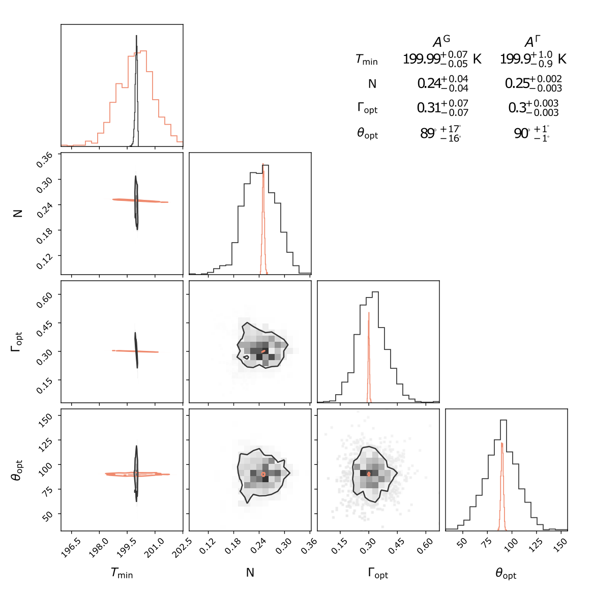
To simulate errors in $\Gamma_{s}$, we generated normally-distributed 0.1 dB magnitude and $1^{\circ}$ phase offsets, then computed error-corrupted noise vectors $\tilde{{\textbf{{x}}}}$ via:

where $\tilde{{\textbf{{A}}}}$ is the source matrix with errors. This approach is similar to that used by NIST (NIST) for noise parameter uncertainty analysis [18]. We ran this procedure 1024 times, then formed scatterplot matrices of noise parameter estimates (Figure 2); the scatterplot shows the covariance between parameters. We find that the traditional approach with ${\textbf{{A}}}^{G}$ exhibits order-of-magnitude larger uncertainties in the retrieved values for $N$, $|\Gamma_{{\rm opt}}|$ and $\theta_{{\rm opt}}$, but smaller uncertainties on $T_{{\rm min}}$ (i.e. if covariance is ignored). We conclude that the removal of the singularity as $\left|\Gamma_{s}\right|\rightarrow 1$ does indeed lead to smaller errors due to matrix inversion.

In the previous section, we showed that for a given four-point pattern, using ${\textbf{{A}}}^{\Gamma}$ in lieu of ${\textbf{{A}}}^{G}$ leads to smaller errors. Here, we discuss the use of four-point patterns comprised of highly-reflective sources, which cannot be used with ${\textbf{{A}}}^{G}$.

The use of open and short impedances ($\Gamma_{{\rm op}}=1$ and $\Gamma_{{\rm sh}}=-1$ ) is well motivated by previous four-point studies, which found that measurement errors are minimized when the phase of $\Gamma_{s}$ is $0^{\circ}$, or $180^{\circ}$ for three of the impedances [6, 7, 8]. In particular, HB16 identifies four regions on the Smith chart in which measurements should be made: regions “B” and “C” contain open and short loci, but the $|\Gamma|<0.9$ requirement precluded their use.

While using open and short maximizes $|$det$|$ of A, leading to smaller matrix inversion errors, we must also consider the measurement accuracy for $\Gamma_{s}$. In general, fractional $S_{11}$ measurement uncertainties on a given VNA are greater for highly-reflective sources; this is a separate error term that runs counter to maximizing $|$det$|$. Fortunately, physical models of short and open are provided by calibration kit manufacturers, and methods for precise and accurate measurement of these standards are well understood [19, 20]. As such, physical models of open and short sources can be used to characterize $\Gamma_{\rm{open}}$ and $\Gamma_{\rm{short}}$, to precision exceeding that possible by VNA measurement alone.

Let us consider the case where ideal open, short and load ($\Gamma_{{\rm ld}}=0$) are used as reference sources, along with an open 1/8-wavelength cable. A lossless open (or shorted) 1/8-wavelength cable introduces a $90^{\circ}$ phase shift (or $-90^{\circ}$), such that $\Gamma_{{\rm cbl}}=\pm 1j$.

For these four references, ${\textbf{{A}}}^{\Gamma}$ is

Note the entry $A_{44}=-2$ if an open cable is used, or $+2$ if a shorted cable is used. ${\textbf{{A}}}^{\Gamma}$ is invertible, with $|$det$|$=32 and condition number $c_{A}=5.62$. The inverse $\text{(${\textbf{{A}}}^{\Gamma}$})^{-1}$

From this, the solutions to ${\textbf{{x}}}={\textbf{{A}}}{\textbf{{t}}}^{\prime}$ are

from which we note that 1) $b$ and $c$ are directly given by the measurement of short and open standards, respectively; and 2) the load measurement is only required to compute $T_{{\rm min}}$, as the A term only appears in Equation 22.

The matrix in Equation 28 is only correct at a central frequency $f_{0}=v_{c}/\lambda_{0}$. For a 1/8-wavelength cable at a central frequency $f_{0}=v_{c}/\lambda_{0}$, we can enforce a minimum $|$det$|$ for the ${\textbf{{A}}}^{\Gamma}$ matrix, and find a fractional bandwidth over which our $|$det$|$ requirement is satisfied. The phase of $\Gamma_{{\rm cbl}}$ is given by $\theta(f)=4\pi L/v_{c}f$, where $v_{c}$ is the velocity factor of the cable. Setting $|$det$|$_min=10, based on the recommendation of SUT20, we compute a corresponding frequency range $f_{{\rm low}}$ to $f_{{\rm high}}$ :

Or put another way, $f_{{\rm high}}=9f_{{\rm low}}$, covering a 9:1 band. For example, if $f_{0}=1$ GHz, then the range over which $|$det$|$ $>$10 is 0.2–1.8 GHz.

In this section, we present a practical method for noise parameter extraction via the use of a load, open, short, and an open 1/8-wavelength cable. In this method, which we call “OSLC”, we form a measurement vector $\text{{{{t}}}'},$which includes a $(1-\left|\Gamma_{s}\right|^{2})$ term that naturally arises when measuring the output power of a 2-port DUT. This term cancels out the singularities inherent in previous methods that use matrices ${\textbf{{A}}}^{\Gamma}$ and ${\textbf{{A}}}^{G}$.

The OSLC method relies on the matrix ${\textbf{{A}}}^{\Gamma}$ (introduced in Section 3), and requires the following:

• •

  A calibrated noise source to generate “hot” and “cold” temperature references, $T_{{\rm hot}}$ and $T_{{\rm cold}}$. The reflection coefficients, $\Gamma_{{\rm hot}}$ and $\Gamma_{{\rm cold}}$ must be known or measured, and should satisfy $\Gamma_{{\rm hot}}\approx\Gamma_{{\rm cold}}$.

• •

  A broadband load, open, and short, with known or measured reflection coefficients $\Gamma_{{\rm ld}}$, $\Gamma_{{\rm op}}$, and $\Gamma_{{\rm sht}}$. Additionally, an open cable (or other mismatch device) with $\Gamma_{{\rm cbl}}\approx\pm 1j$. To minimize pickup of radio interference, we recommend that the cable is placed inside an RF-shielded box with an SMA feedthru connection.

• •

  A radio receiver to measure power spectral density (PSD) with linear response. The input reflection coefficient $\Gamma_{{\rm rx}}$ should be known or measured, and the receiver must have high reverse isolation ($S_{12}S_{21}\approx 0$) for the analog component before the digitizer.

• •

  A 2-port VNA to measure the S-parameters of the DUT, and any unknown reflection coefficients. However, If the DUT is highly directional and well-matched to the receiver – such that $\left|S_{12}S_{21}\Gamma_{rx}\right|\approx 0$ – only $S_{11}$ is required.

To show how the OSLC approach may be used, let us start by considering a power measurement made by a radio receiver. The power $P_{s}$ measured at the output of a 2-port network with scattering matrix [$S$], connected to a source impedance $Z_{s}$ and load impedance $Z_{{\rm rx}}$ (see Figure 1), is given by

where $k_{B}$ is the Boltzmann constant, $\Delta f$ is the noise equivalent bandwidth, $T_{n}$ is the noise temperature of the DUT (when connected to $Z_{s}$ and $Z_{{\rm rx}}$), $T_{s}$ is the noise temperature of the source ($T_{s}=T_{{\rm amb}}$ for passive networks at ambient temperature), and $\mathcal{G}_{{\rm DUT}}=\mathcal{G}_{{\rm DUT}}(Z_{s})$ is the available gain of the DUT. Here, $\mathcal{D}_{{\rm rx}}$ encompasses all (unknown) digital conversion and gain factors within the receiver, assumed to be linear.

The available gain [21], denoted here with $\mathcal{G}$, of the DUT is given by

When connected to the source impedance $Z_{s}$, the two-port network will be mismatched with a reflection coefficient, $\Gamma_{{\rm out}}(Z_{s})$:

For a calibrated noise source with low reflection coefficient, and requiring $\Gamma_{{\rm hot}}\approx\Gamma_{{\rm cold}}$, we define $\Gamma_{{\rm ns}}=(\Gamma_{{\rm hot}}+\Gamma_{{\rm cold}})/2$. It follows that the ratio

Where $\mathcal{G}_{\rm{rx}}$ is the available gain of the receiver’s analog components. Referring to Figure 1, the receiver sees an input impedance $\Gamma_{{\rm DUT}}=\Gamma_{{\rm out}}(Z_{s})$, which depends upon the source impedance $Z_{s}$. So, the total cascaded gain (as seen at the receiver output) is given by $\mathcal{G}_{{\rm casc}}(Z)=\mathcal{G}_{{\rm DUT}}(Z)\mathcal{G}_{{\rm rx}}(Z_{{\rm out}})$. For a receiver (with high reverse isolation), the ratio

We now define a scale factor $\alpha$, which converts from power to temperature units, and a mismatch factor $M_{s}$ (similar to Eq. 30 of [14]):

and from Equation 35 we retrieve

Note that the terms $\mathcal{G}_{{\rm DUT}}^{-1}$ and $T_{{\rm rx}}$ are dependent upon the source impedance ($Z_{s}$); however, for sources where $\left|\Gamma_{s}\right|\approx 1$ and/or $\mathcal{G}_{{\rm DUT}}$ is large, the factor can be discarded, simplifying to:

We may now form the measurement vector ${\textbf{{t}}}^{\prime}$ by applying calibration Equation 42 to our measured power $P_{s}$:

Specifically, if we connect a load, open, short, and a (lossless) open 1/8-wavelength cable to a DUT, the noise parameters are retrieved via

where $\text{(${\textbf{{A}}}^{\Gamma}$})^{-1}$ is given by Equation 28; note that $M_{{\rm ld}}\approx 1$.

We applied our technique to measure the noise parameters of a Minicircuits ZX60-3018G-S+ amplifier, across 50–250 MHz. The amplifier has a manufacturer-supplied noise figure of 2.7–2.9 dB across the 50–250 MHz band, and a gain of $\sim 25.5$ dB. Here, we used an SMA-terminated 15-cm RG-400 coaxial cable, with $v_{c}\approx 0.69.$ Based on Equations 33 and 34, the nominal frequency range for this cable is $\sim$30–300 MHz. The $|$det$|$ for the ${\textbf{{A}}}^{\Gamma}$ matrix using an open, short, load, and 15-cm cable, is shown as a function of frequency in Fig 4.

To generate hot and cold reference loads, we used a Keysight HP346A noise source with an ENR of 5.56–5.49 dB across 10 MHz to 1 GHz. As ENR is only quoted at intervals, we use a 2-order polynomial fit to generate values across 50–250 MHz.

Measurements of power spectra were generated using a custom receiver, based on a 14-bit Signatek PX1500-2 analog to digital converter (ADC) running at 650 Msamples/s; the noise performance of the receiver was characterized prior to measurement. Power spectra were generated from ADC samples via an autocorrelation spectrometer, which applies a 4096-channel Fast Fourier Transform (FFT), signal detection, and time averaging. The receiver has a pair of Minicircuits ZFL-500HLN+ amplifiers to provide an extra $\sim 38$ dB of gain before digitization, and a 50-MHz highpass filter (Minicircuits SHP-50+) and K&L Microwave 300-MHz lowpass filter were added at the ADC input as an anti-aliasing filter. The receiver temperature, $T_{\rm{rx}}$, is 1350–1450 K across the band. We captured 60 s of data per measurement.

To measure reflection coefficients of the DUT, load, cable, and the receiver, we used a Fieldfox N9915A VNA, calibrated with an Agilent 85052D calibration kit. Passive components were measured using a high (0 dBm) port power, whereas lower power (-30 dBm) was used to measure the [$S$] matrix of the DUT and $\Gamma_{{\rm rx}}$. Measurements were saved in S2P (Touchstone) format, and read using the Python package scikit-rf²² 2 www.scikit-rf.org. To determine $\Gamma_{{\rm sh}}$ and $\Gamma_{{\rm op}}$, we used a physical model based on the Agilent 85052D calibration standard definitions (see Appendix C).

Figure 5 shows the measure power $P_{s}$ for the DUT with the load, open short and cable reference sources (top panel). The computed mismatch factors $M_{s}$ (Equation 41) which are applied during calibration (Equation 42) are shown in the middle panel, and calibrated entries to the vector ${\textbf{{t}}}^{\prime}$ are shown in the bottom panel.

Based on the measurement vector ${\textbf{{t}}}^{\prime}$ and $4\times 4$ matrix ${\textbf{{A}}}^{\Gamma}$, we solve for the noise parameter vector x (Equation 20) via matrix inversion ${\textbf{{x}}}=\text{(${\textbf{{A}}}^{\Gamma}$})^{-1}{\textbf{{t}}}^{\prime}$ . We then solve for the standard noise parameters via Equations 22–25. The derived noise parameters $T_{{\rm min}}$, $N$, and $\Gamma_{{\rm opt}}$ are shown in Figure 6. Errors are derived using the Monte Carlo approach detailed in Section V, assuming VNA measurements of the coaxial cable are accurate to $\pm 0.1$ dB in magnitude and $0.5^{\circ}$ in phase. Errors on the open, short and load impedance are modelled as gaussian random variables, with uncertainties based upon manufacturer-supplied electrical specifications [22].

Also plotted in Figure 6 are measurements from SUT20 [14, Fig 12] of the same amplifier model. The authors followed a different measurement methodology, involving a Focus Microwaves CCMT-101 single-probe slide screw tuner and Keysight PXA N9030A receiver. Note that 1) while the model is identical, we did not use the same DUT and 2) uncertainties in SUT20 were derived using a different approach, so cannot be directly compared. Nevertheless, our results are in close agreement with those presented in SUT20. A $\approx 15^{\circ}$ offset between $\theta_{\rm{opt}}$ is apparent, which could be due to variation between amplifiers or differences in operating conditions.

Here, we have shown that the commonly-used admittance-based matrix ${\textbf{{A}}}^{G}$, after removal of its singularity, can be rewritten as simple expression of reflection coefficients (${\textbf{{A}}}^{\Gamma}$, Equation 18). We also show that uncertainties in noise parameter estimates due to errors in the source impedance matrix A are significantly lowered by using ${\textbf{{A}}}^{\Gamma}$ instead of ${\textbf{{A}}}^{G}$. Combined, these suggest that singularity-free formulations of A should be used where possible.

We have presented a straightforward method to measure noise parameters using a broadband load, open, short, and 1/8-wavelength cable as reference sources (“OSLC”). Our method leverages a singularity-free matrix, to allow the use of highly reflective reference loads. Specifically, our method allows for open and short calibration standards to be used as reference sources.

The ability to use highly reflective reference loads allows the spread of loci in the Smith chart to be maximized, which also maximises $|$det$|$, the magnitude of the matrix determinant. It follows that highly-reflective references will yield lower worst-case scaling errors due to matrix inversion. However, the use of highly-reflective sources requires that the DUT is unconditionally stable. Also, VNA measurements of highly-reflective sources are prone to larger fractional errors (the magnitude of which depend upon VNA specifications and calibration approach). Physical models of open and short circuits, as provided in VNA calibration kits, can be used in lieu of VNA measurements and are more accurate; methods for precise characterization of high-impedance references can also be employed [19, 20].

The OSLC four-point method can be used across a range 0.2–1.8$\lambda_{0}$, for a cable of length $\lambda_{0}/8$. If a larger range is required, one could use a set of cables with varying lengths and repeat the process at different central frequencies. Alternatively, rows may be added to ${\textbf{{A}}}^{\Gamma}$ and the pseudoinverse may be used when solving (Equation 5).

The OSLC method is well-suited to low-frequency application ($<$1 GHz), as the only source impedances are a 1/8-wavelength cable and a VNA calibration kit: both are accessible and affordable. Approaches that leverage rapid phase wrapping [9, 10, 13] may require lengths of cable that are unwieldy or prohibitively long at low frequencies. Admittance tuners, which are rated down to a half-wavelength, are comparatively expensive and physically bulky.

The OSLC method is more practical than previous approaches for in-situ measurement in the field using a portable VNA and spectrum analyzer. On the flip side, at higher frequencies, a 1/8-wavelength cable may become prohibitively small. Precision airlines offer very low loss and may be a suitable alternative; nevertheless, further research is needed to validate comparable methodologies at millimeter frequencies. Modifications to the approach may also be needed for single-transistor DUTs, which can be poorly matched at low frequencies.

The authors would like to thank Budi Juswardy, Dave Kenney and Daniel Ung for help with laboratory measurements. This research made use of Scikit-RF, an open-source Python package for RF and Microwave applications, and Corner.py [23]. All calculations were performed in Python 3.7, using the Numpy package [24].

References

- [1] H. A. Haus et al., “Representation of noise in linear twoports,” Proceedings of the IRE, vol. 48, no. 1, pp. 69–74, 1960.
- [2] R. Meys, “A wave approach to the noise properties of linear microwave devices,” IEEE Trans. Microw. Theory Techn., vol. 26, no. 1, pp. 34–37, 1978.
- [3] S. Wedge and D. Rutledge, “Wave techniques for noise modeling and measurement,” IEEE Trans. Microw. Theory Techn., vol. 40, no. 11, pp. 2004–2012, 1992.
- [4] R. Lane, “The determination of device noise parameters,” Proceedings of the IEEE, vol. 57, no. 8, pp. 1461–1462, 1969.
- [5] A. Davidson, B. Leake, and E. Strid, “Accuracy improvements in microwave noise parameter measurements,” IEEE Trans. Microw. Theory Techn., vol. 37, no. 12, pp. 1973–1978, 1989.
- [6] S. Van den Bosch and L. Martens, “Improved impedance-pattern generation for automatic noise-parameter determination,” IEEE Trans. Microw. Theory Techn., vol. 46, no. 11, pp. 1673–1678, 1998.
- [7] M. De Dominicis, F. Giannini, E. Limiti, and G. Saggio, “A novel impedance pattern for fast noise measurements,” IEEE Trans. Microw. Theory Techn., vol. 51, no. 3, pp. 560–564, 2002.
- [8] M. Himmelfarb and L. Belostotski, “On impedance-pattern selection for noise parameter measurement,” IEEE Trans. Microw. Theory Techn., vol. 64, no. 1, pp. 258–270, 2016.
- [9] R. Hu and S. Weinreb, “A novel wide-band noise-parameter measurement method and its cryogenic application,” IEEE Trans. Microw. Theory Techn., vol. 52, no. 5, pp. 1498–1507, 2004.
- [10] A. E. E. Rogers and J. D. Bowman, “Absolute calibration of a wideband antenna and spectrometer for accurate sky noise temperature measurements,” Radio Science, vol. 47, no. 6, 2012. [Online]. Available: https://agupubs.onlinelibrary.wiley.com/doi/abs/10.1029/2011RS004962
- [11] H. Friis, “Noise figures of radio receivers,” Proceedings of the IRE, vol. 32, no. 7, pp. 419–422, 1944.
- [12] V. Adamian and A. Uhlir, “A novel procedure for receiver noise characterization,” IEEE Trans. Microw. Theory Techn., vol. 22, no. 2, pp. 181–182, 1973.
- [13] I. L. V. Roque, W. J. Handley, and N. Razavi-Ghods, “Bayesian noise wave calibration for 21-cm global experiments,” Monthly Notices of the Royal Astronomical Society, vol. 505, no. 2, pp. 2638–2646, Aug. 2021.
- [14] A. T. Sutinjo, L. Belostotski, B. Juswardy, and D. X. C. Ung, “A measure of well-spread points in noise wave-based source matrix for wideband noise parameter measurement: The ska-low example,” IEEE Trans. Microw. Theory Techn., vol. 68, no. 5, pp. 1783–1793, 2020.
- [15] A. T. Sutinjo and L. Belostotski, “Analytical determinant of the noise parameter extraction matrix and its applications,” in 2019 USNC-URSI Radio Science Meeting (Joint with AP-S Symposium), 2019, pp. 81–82.
- [16] M. Lefebvre, R. K. Keeler, R. Sobie, and J. White, “Propagation of errors for matrix inversion,” Nuclear Instruments and Methods in Physics Research A, vol. 451, no. 2, pp. 520–528, Sep. 2000.
- [17] L. Belostotski and J. W. Haslett, “Evaluation of tuner-based noise-parameter extraction methods for very low noise amplifiers,” IEEE Trans. Microw. Theory Techn., vol. 58, no. 1, pp. 236–250, 2010.
- [18] J. Randa, “Numerical modeling and uncertainty analysis of transistor noise-parameter measurements,” International Journal of Numerical Modelling: Electronic Networks, Devices and Fields, vol. 28, no. 6, pp. 628–638, 2015. [Online]. Available: https://onlinelibrary.wiley.com/doi/abs/10.1002/jnm.2039
- [19] J. Dunsmore, Handbook of Microwave Component Measurements: With Advanced VNA Techniques. Wiley, 2012.
- [20] R. A. Monsalve, A. E. E. Rogers, T. J. Mozdzen, and J. D. Bowman, “One-Port Direct/Reverse Method for Characterizing VNA Calibration Standards,” IEEE Transactions on Microwave Theory Techniques, vol. 64, no. 8, pp. 2631–2639, Aug. 2016.
- [21] D. Pozar, Microwave Engineering, 4th Edition. Wiley, 2011. [Online]. Available: https://books.google.com.au/books?id=JegbAAAAQBAJ
- [22] n.d., “Keysight 85052d 3.5 mm economy calibration kit user’s and servrice guide,” Keysight, Tech. Rep., 2014.
- [23] D. Foreman-Mackey, “corner.py: Scatterplot matrices in python,” The Journal of Open Source Software, vol. 1, no. 2, p. 24, Jun 2016.
- [24] C. R. Harris et al., “Array programming with NumPy,” Nature, vol. 585, no. 7825, pp. 357–362, Sep. 2020. [Online]. Available: https://doi.org/10.1038/s41586-020-2649-2
- [25] D. C. DeGroot, K. L. Reed, and J. A. Jargon, “Equivalent circuit models for coaxial oslt standards,” in 54th ARFTG Conference Digest, vol. 36, 2000, pp. 1–13.
- [26] n.d., “Application note 1287-11: Specifying calibration standards and kits for agilent vector network analyzers,” Agilent, Tech. Rep., 2011.
Appendix A Derivation of
To show that , we note that