Design and characterization of cochlea-inspired tonotopic resonators
Abstract
The cochlea has long been the subject of investigation in various research fields due to its intriguing spiral architecture and unique sensing characteristics. One of its most interesting features is the ability to sense acoustic waves at different spatial locations, based on their frequency content. In this work, we propose a novel design for a tonotopic resonator, based on a cochlea-inspired spiral. The resulting structure was subjected to an optimization process to exhibit out-of-plane vibration modes with mean out-of-plane displacement maxima distributed along its centerline spanning nearly a two-decade frequency range. Numerical simulations are performed to demonstrate the concept, which is also confirmed experimentally on a 3D printed structure. The obtained frequency-dependent distribution is shown to be a viable source of information for the discrimination of signals with various frequency components. The harnessed tonotopic features can be used as a fundamental principle to design structures with applications in areas such as non-destructive testing and vibration attenuation.
Keywords:
Bio-inspired metamaterial; Cochlea; Tonotopy; Resonators.1 Introduction
Among the various sensory organs developed in nature over the course of evolution, the cochlea is certainly one of the most fascinating dallos2012cochlea. This coiled structure possesses unique characteristics which allow mammalians to perceive sounds in wide frequency and amplitudes ranges, comprising nearly ten octaves and decibels robles2001mechanics. As one of the many examples of naturally-occurring spiral structures livio2008golden, the cochlea can be approximately modeled by considering a logarithmic spiral description, first presented by Dürer durer1525underweysung, which can be used to investigate the influence of geometrical features on its frequency-dependent characteristics manoussaki2008influence. Beyond the obvious advantages offered by structural coiling in terms of packing, the cochlea also possesses tonotopic characteristics, i.e., where the intensity of the mechanotransduction responsible for converting sound energy into neural impulses varies with the location of peak excitation lemasurier2005hair. Such space-dependent detection of mechanical signals based on their frequency content provides unique frequency detection attributes that are essential for hearing lighthill1991biomechanics.
The design concepts present in the cochlea are also of considerable interest in the field of bio-inspired metamaterials, usually employing locally resonant structures able to mimick the tonotopy observed in the cochlea ma2016cochlear, rupin2019mimicking. The use of locally resonant structures is widespread in the context of wave manipulation, ever since the seminal work presented by Liu et al. liu2000locally opened new possibilities for the development of locally resonant phononic crystals kushwaha1994theory, laude2020phononic, with one- xiao2013theoretical, xiao2013flexural, dal2019optimization, two- xiao2012flexural, miranda2019flexural, poggetto2021flexural, and three-dimensional applications mitchell2014metaconcrete, witarto2019three, dal2020elastic. These structures present as a typical characteristic local resonance band gaps bloch1929quantenmechanik, which are frequency bands that strongly attenuate wave propagation and can occur at sub-wavelength dimensions krushynska2017coupling. Also, in contrast with the typical band gaps observed in phononic crystals, occurring due to Bragg scattering gorishnyy2005sound, local resonance band gaps do not strictly require the periodicity of the medium to emerge, thus avoiding the necessity of using many unit cells to achieve a noticeable effect.
The width of local resonance band gaps, on the other hand, is typically much narrower than Bragg scattering band gaps krushynska2017coupling. To overcome this drawback, a possible approach is to combine several elements with distinct resonant frequencies to create a rainbow effect able to encompass a wider frequency range de2021selective. The experimental realization of structures able to achieve this effect, however, may be complicated, since it requires the combination of multiple elements meng20203d. Approaches considering structures able to separate frequencies along their spatial profile for impinging acoustic waves have been proposed in linear zhu2013acoustic and coiled structures ni2014acoustic, but to the best of our knowledge, no similar designs were attempted considering elastic waves propagating in a solid medium. Therefore, the current state-of-art lacks the development of a structure which can be used with the same simplicity as that of a tuned resonator jin2017pillar, but does not suffer the drawbacks of being restricted to a limited number of resonant frequencies, thus presenting the advantages of the rainbow-like effect which is associated with the utilization of a cochlear geometry.
The numerical and experimental results presented herein demonstrate how a cochlea-inspired tonotopic resonator can be used as a single resonant element with tailored resonant frequencies able to span a wide frequency range, thus expanding the possibilities of wave manipulation and control, with relevant technological use involving mechanical vibrations, such as sensing applications pennec2019phononic and energy harvesting carrara2013metamaterial, qi2016acoustic, chaplain2020topological, de2020graded, de2020experimental, lin2021piezoelectric.
The paper is organized as follows. In Section 2, the geometrical model for the development of the cochlea-inspired resonator is presented, along with relevant metrics which are useful to investigate the spatial distribution of energy according to the variation of natural frequencies, i.e., the tonotopic energy profile. The numerical and experimental results illustrating the tonotopic behavior of the proposed curved structure are presented in Section 3. Concluding remarks are presented in Section 4.
2 Models and methods
2.1 Geometric properties
The cochlea-inspired curved structure is here modeled by sweeping a rectangular cross section (width and height, respectively) along a centerline curve, , described in a cylindrical coordinate system (Figure 1a). The mass density of the structure is taken as constant. A logarithmic spiral can be written in these coordinates as
| (1) |
where is the initial radius of the spiral, , represents the constant polar slope of the spiral, and is the maximum angular coordinate for a number of turns of the cochlea. Planar cochleae are represented by the simplification . The arc length can be computed using the line integral over the radius function in Eq. (1) as
| (2) |
which, for the case of , simplifies to
| (3) |
thus leading to the centerline normalized coordinate , described as
| (4) |
Analogously, the cross section dimensions of the cochlea, and , can be written as
| (5) |
with and representing, respectively, the initial width and height of the cochlea cross section, and and associated with the variation of the width and height, respectively. These equations can also be expressed in terms of the normalized coordinate using Eq. (4):
| (6) |
thus indicating the explicit dependence of () on the ratio (), which can be varied to tune the geometric parameters of the spiral.
The parameters and can be defined by specifying the cochlea cross section at , i.e., and . An example of a cochlea constructed using this approach is shown in Figure 1b. Also, special care must be taken so that overlapping does not occur (i.e., the cochlea does not self-intersect, see Figure 1c).
The volume of the resulting cochlea is calculated as
| (7) |
where can be regarded as a dimensionless shape factor.

For simplicity, let us assume a planar cochlea. The gap in the radial direction between two adjacent turns is given by
| (8) |
where and are the inner and outer radii of the cochlea, respectively, for the angular coordinate . Although the condition is theoretically possible, it implicates in surface contact and manufacturing issues. Thus, the condition of no overlapping is achieved for , , which can be related with a minimum gap value () as
| (9) |
which, combined with Eqs. (1) and (5), yields the condition
| (10) |
2.2 Tonotopic modal profiles
As a reference case, we initially consider a rectangular prism with dimensions with . The resonant frequencies and corresponding modes of vibration of this element can be obtained for a given set of boundary conditions. If one considers, for instance, free boundary conditions for all of its faces, the first modes (excluding rigid-body motion) are depicted in Figure 2a, with the color bar representing the absolute value of displacements. At this point, no specific material properties are specified, since the presented concepts are general.
The representation of each separate eigenmode, however, may become increasingly difficult for large sets. Thus, it may be useful to summarize the information contained in each eigenmode in a concise manner.
This can be done, for instance, by considering the eigenmode displacements in a given direction, e.g., out-of-plane displacements (), and calculating an associated quadratic displacement cross-section mean (mean displacement for short), , computed over its transverse directions ( and ), written as
| (11) |
where is the cross section at coordinate , denotes the complex conjugate operator and can be calculated for each eigenmode, previously normalized with respect to its largest computed displacement. Out-of-plane direction displacements are chosen due to (i) a biological motivation, since such displacements are analogous to the direction in which the cochlea basilar membrane is coupled with the surrounding fluid, and (ii) an experimental motivation, since out-of-plane velocities can be directly measured in an experimental setup. The quantity can be computed for a set of resonant modes of a given frequency range of interest, thus yielding a tonotopic modal profile () for this frequency range. An example of the obtained tonotopic modal profile is given in Figure 2b using a perspective view. The top view of the same profile, shown Figure 2c, is useful to graphically illustrate the characteristics of the various resonance modes. For example, the lateral mode does not appear, since it has a zero value for out-of-plane displacements, while the bending higher order modes display a larger number of local maxima compared to the lower order bending modes.

2.3 Effects of variations in thickness or width
The symmetry in the distribution of maxima along the element length (see Figure 2c) is due to the overall distribution of energy for each frequency. However, this symmetry can be manipulated through the control of geometric properties such as the variation of width, thickness, and the boundary conditions to which the element is subjected. To illustrate these effects, consider elements with variation in their width (Figure 3a) or thickness (Figures 3b). For each case, we display the distribution of mean displacements and their maxima for free-free and clamped-clamped boundary conditions. For instance, considering the clamped-clamped boundary conditions, creating an asymmetry in the geometric and mechanical properties of the structures allows to manipulate the distribution of energy for each mode of vibration so that maxima vary spatially according to each resonant frequency, thus inducing a tonotopic effect. The maxima, however, do not present a uniform distribution along the length of the structure, and are rather confined to a small region towards the end of the element.
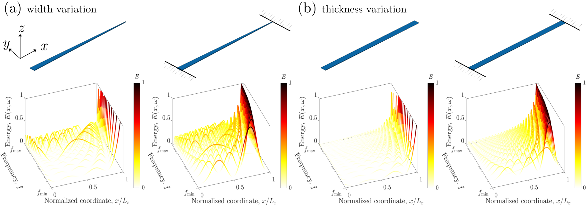
In the next section, we present numerical results that demonstrate how tonotopic effects can be achieved using curved structures, additionally obtaining that the maxima of the vibration modes follow a desired spatial distribution.
3 Tonotopic effects in curved structures
The numerical results presented in this section are computed considering the material properties of a polymer used in Section 3.4 for 3D-printing processes (Solflex SF650, W2P Engineering GmbH), with Young’s modulus GPa, Poisson’s ratio , and mass density kg/m3. The frequency range of interest is restricted to Hz, thus encompassing a two-decade range. For the considered material properties and an initial thickness of mm, the smallest flexural wavelength at is equal to mm.
3.1 Curved profiles
The following geometries and distribution of mean out-of-plane displacement maxima are computed as previously using the finite element method, considering isoparametric hexahedral elements with linear elastic behavior cook2001concepts, bathe1996finite, ferreira2010matlab. An initially straight, regular node grid is mapped into a curved structure according to the geometric parameters to generate the volume described by Eqs. (1), (5), and (8). The and faces are mapped into the inner () and outer () faces, respectively, while the and faces are mapped into the lower () and upper () faces of the curved structure, respectively. Likewise, the -coordinates of the initially straight solid element are mapped on to the coordinate using the linear relation .
The boundary conditions are considered as clamped at the face with largest width of the cochlea () and free at the other end (), thus representing the attachment of the structure to an ideally infinitely stiff substrate. The previously presented quadratic displacement mean metric (Eq. (11)) is approximated for the use with the finite element discretization considering the sum in the radial and vertical directions, i.e.,
| (12) |
where and are the number of nodes considered in the finite element model in the radial and vertical directions for a given coordinate, respectively.
A baseline structure, shown in Figure 4a, is obtained by initially considering the dimensions mm and mm . The spiral parameters are set as , (thus yielding a reduction to of the initial width), (fixed thickness), a minimum gap of mm, and a total of turns. The distribution of mean displacement maxima, indicated in Figure 4b, presents considerable tonotopy, with a noticeable separation between the peak for each mode up to kHz (as indicated by the black dashed fitting line in Figure 4c), where the bending modes (A and B, Figure 4d) are clearly distinguishable. Above this frequency, the maximum of each eigenmode occurs at , thus losing tonotopy. Also, for higher frequencies, higher-order bending modes in the radial direction (which can also be interpreted as torsional in the circumferential direction) may occur (modes C and D, Figure 4d), thus hindering the desirable clear visualization of tonotopy.

To investigate the effect of the geometric parameters that describe the coiling (, ), thickness (), and number of turns () of the cochlea, three additional structures are proposed, obtained by increasing either (i) the number of turns while keeping the same final width (, Figure 5a), (ii) the coiling of the spiral (, Figure 5b), or (iii) the variation of thickness (, Figure5c), while fixing the other parameters.
The distribution of mean displacement maxima obtained for an increased number of turns, shown in Figure 5d), indicates that the smooth transition in the curved structure cross section hinders the formation of isolated peaks for each resonant frequency due to a more uniform distribution of maxima along the circumferential direction for each resonant frequency.
An increase in the coiling of the structure, on the other hand, seems to be highly beneficial for a tonotopic effect in the structure, as shown in Figure 5e, since the peaks corresponding to each mode show a good contrast with other maxima and also a noticeable isolation. The tuning of the structure eigenmodes through these parameters, however, may be hard to achieve in terms of manufacturing, due to the need to create extremely small parts in the resulting structure. This limitation can, however, be alleviated by an increase in the thickness of the structure, which provides similar effects as the increase in the coiling of the structure (Figure 5f).

It is known that in the actual cochlea, low frequencies are mostly detected in the inner part, and high frequencies in the outer part reichenbach2014physics. The opposite happens for elastic wave propagation in the structures considered up to this point. However, this is not necessarily true in all cases. Consider, for example , a structure obtained through the same previously described process, but stiffer at its outer edge () and more flexible at the inner edge (), thus inducing, respectively, high- and low-frequency resonant frequencies in these regions.
To this end, let the geometrical control parameters be , , and . Also, all edges of the structure are considered as clamped to account for the stiffness of the surrounding medium supporting the basilar membrane in the cochlea. In this case, we also consider larger dimensions to obtain resonant frequencies comparable with the previous examples, using mm, mm, mm, mm, and turns.
These parameters result in the structure presented in Figure 6a, occupying an area of approximately mm2. The associated tonotopic modal profile is shown in Figure 6b, with a limit curve (, dashed green line) indicating the location of local maxima, which confines the elastic energy at the region delimited by for each resonant frequency. Wave modes marked as A–D are displayed in Figure 6c, indicating that the locations of maximum displacement move from the inner to the outer region of the cochlea as the frequency increases, as expected. For lower frequencies, the points of maxima are quite noticeable.
Although this type of structure may be interesting for certain applications and demonstrates the versatility of the proposed approach, it suffers from drawbacks such as (i) the considerable presence of void spaces in the in-plane design, thus leading to a low efficiency in the use of space, (ii) the large dimensions associated with the final structure, and (iii) the poor discrimination between maxima, which possibly hinders the use of the structure in sensing applications.

3.2 Optimization of tonotopy
The results from the last section show that the manipulation of tonotopy can be achieved by varying the geometric parameters that control the curvature, width, and thickness of the cochlea. The parameters that control the curvature and number of turns, however, may lead to prohibitively small features, which can be difficult in terms of manufacturing, thus suggesting that optimal values can be obtained considering practical manufacturing limitations.
To better evaluate and quantify the level of ideal tonotopy presented by the structure, we propose a metric () defined as
| (13) |
where represents the distance between the maximum of the mean displacements computed for the -th out-of-plane vibration mode and the line, as illustrated in Figure 7a, calculated considering the normalized coordinate and the normalized frequency , for and . The line is considered as the ideal distribution of modes maxima, since it covers the entire physical and considered frequency ranges with an uniform distribution. The combination of the objective function and the restrictions on variables , , and yields a constrained nonlinear optimization problem, which is solved using an active set algorithm wright1999numerical, which can be implemented in Matlab matlaboptimization to obtain global optimal solutions.
For the present problem, we considered turns and a minimum gap of mm (see Eq. (10)), restricting the optimization parameters to , , and . The optimization results yield , , and . Very similar results were obtained when considering normalized coordinates instead of in the optimization metric given by Eq. (13). It is interesting to notice that is equal to the lower boundary of the variable, yielding a quasi-linear width decrease in the -coordinate (, see Eq. (6)), while the height increase is steeper, equal to the upper boundary of the variable (, see Eq. (6)). The resulting structure is shown in Figure 7b, and the corresponding distribution of mean displacement maxima is shown in Figures 7c and 7d for the clamped-free and free-free boundary conditions, respectively, indicating a significant correlation when considering the normalized coordinates.

3.3 Numerical demonstration of tonotopy
The tonotopy of the resulting structure is also demonstrated by a numerical simulation where transient signals are considered. The obtained structure, shown in Figure 7b, is attached to a square platform of dimensions mm2, to which a “burst” signal is applied, as depicted in Figure 8a.
For the definition of the input signal, a set of fundamental frequencies () is considered. For each case, the duration of the burst consists of periods, i.e., , with , while the total duration of the signal is (see the inset of Figure 8a). A total of points is considered, thus leading to distinct values of time sampling , which differ due to the large difference between the fundamental frequencies, chosen as Hz. A time-domain transient analysis based on the Newmark method bathe1996finite can then be performed, and the resulting out-of-plane velocity values () computed for the centerline of the sample (green line in Figure 8a). A Fast Fourier Transform (FFT) is applied considering each separate coordinate and plotted using distinct colors for the obtained frequency components (), as shown in Figure 8c.
For the first input frequency, the maximum of out-of-plane mean displacements is located close to , thus resembling the results computed considering the clamped end (Figure 7c). This maximum shifts to higher values of as the input frequency increases, thus clearly demonstrating the effect of tonotopy. Is is also worth noticing that the resolution in the frequency domain, given by , has a smaller value for the signals with lower frequencies ( Hz for Hz) than for those at higher frequencies ( Hz for Hz). An equal number of isofrequency lines are considered for each representation, thus leading to wider depicted frequency ranges for higher input frequencies, which explains the occurrence of multiple resonant frequencies for higher input frequency values, as and Hz.

3.4 Experimental verification of tonotopy
To verify the tonotopy of the designed cochlea and the feasibility of its potential use as a frequency selective device, we performed an experimental realization of the spiral structure obtained by the numerical optimization process and employed in Section 3.3. The structure was printed on a commercial 3D-DLP printer (Solflex SF650, W2P Engineering GmbH) using polymeric resin Solflex Tech Though (from the same manufacturer) with the same mechanical properties as considered in the numerical simulations. The printer is equipped with an UV-LED emitting at a wavelength of nm and with a specified power density of mW/cm2. The nominal lateral resolution is m and the printer supports layer thicknesses ranging from to m. Here, the design was sliced into layers of m, each exposed for s, leading to a dose of mJ/cm2 per layer. The parts were oriented with their -plane parallel to the printing platform such that the slicing was performed along the -axis and were printed standing on a removable support structure to increase the bottom surface smoothness. After printing, the parts were washed with Isopropyl Alcohol (IPA), then fully immersed in IPA and sonicated twice for minutes in an ultrasonic bath (USCTH, VWR International). Finally, they were UV-post-cured for 1 hour in a PHOTOPOL Analog UV-curing unit (Dentalfarm Srl), providing all-around illumination in the wavelength range – nm.
The experimental setup was also similar to the numerical simulation performed in Section 3.3. A piezoelectric transducer, with a diameter of mm and negligible weight with respect to the entire structure, was glued to the external edge of the printed cochlea resonator (see red circle in Figure 9a). A Gaussian shaped burst signal with varying central frequency () was injected with an arbitrary function generator (Agilent 33500), amplified by a factor by a liner amplifier (FLC Electronics, A400DI) and applied to the piezoelectric transducer. The central frequency of the signals varied in the range Hz, with a burst duration of . The experiment was repeated for each frequency , recording the response of the structure in points along the centerline of the cochlea (see blue dots in Figure 9a), using a laser vibrometer (Polytec, OFV-505) to scan the surface of the sample. The vibrometer was placed orthogonal to the plane containing the spiral structure, in order to detect the out-of-plane velocity.
The results of the experiment are reported in Figure 9b, where the normalized amplitude of the velocity signals detected at various different points are reported as a function of the angular position on the cochlea centerline. The different coloured lines, which use the same frequency-based color coding as presented in Figure 8, represent the responses of the structure for different values of the central frequency of the exciting burst and correspond, respectively, to , , , , , , and Hz. Results show that the maximum (highlighted by a colored dot) moves along the cochlea centerline starting from the outer part (maximum radius) to the apex (minimum radius), where higher frequencies are detected. The maxima are well resolved in space, as highlighted by reporting the position of the maximum amplitude on the cochlea centerline (see Figure 9c), and each maximum is unique for a fixed frequency along the cochlea, thus proving the tononotopy of the structure.
By plotting the logarithm of the central frequency as a function of the position of the maximum in the normalized coordinate for a given set of central frequencies, it is possible to recognize a clear correlation with the tonotopic modal profile previously presented in Figure 7c; for greater clarity, results are overlaid in Figure 9d. Also, a functional dependence between the central frequency and its location in the cochlea centerline can be estimated by an exponential fit of the form (see Eq. (4)), with Hz and m-2. In this case, the frequency range is reduced to Hz to allow for single fit, instead of adopting a piecewise function. Also, an additional measurement is performed at Hz (yellow point in Figure 9c) to confirm its closeness to the exponential fit. This fit may allow to identify the optimal position for the detection on the structure of a certain frequency in the range .

3.5 Sensing applications
Having assessed the validity of the tonotopic effect on the optimized spiral structure, we now propose a numerical experiment to demonstrate its possible use in sensing and in non-destructive testing applications. For this purpose, a mm3 beam is attached to the previously designed cochlea and platform structure. The beam is then excited with an out-of-plane point force at mm from the edge of the platform, located at its upper face and applied at its center. Points , , , and , corresponding to the frequencies of Hz, Hz, kHz, and kHz are chosen as outputs. As these frequencies are not necessarily resonant frequencies, the location of the points at the central line of the cochlea are determined by a linear interpolation of the peaks presented in Figure 7c for the coordinate, resulting in the angles , , , and , respectively. The resulting structure is presented in Figure 10a. Distinct input forces with single frequency components are applied for a total of periods (using a discretization of points in the time domain) and a Hanning window (see the inset in Figure 8a), while the output signals are computed for a total of periods. The normalized acceleration output values are presented in Figure 10b. In each case, the single-frequency input signal generates the strongest response at the corresponding output point, i.e., Hz for point P1, Hz for point P2, kHz for point P3, and kHz for point P4. Furthermore, although excitation signals at lower frequencies still produce a considerable response at the high-frequency output points (e.g., the output at P4 is appreciable even for the Hz input signal), this effect is much less pronounced at higher frequencies. In particular, for an input frequency of kHz, the output accelerations at points P1 – P3 are considerably smaller than at P4, which can be explained by the localization of out-of-plane mean displacements of higher frequency wave modes.

As a second application, let us now consider the problem of determining the frequency content of a signal () containing multiple harmonics, which may derive, for instance, from nonlinearities. Let us define such a signal as , for , which is applied as the input force of the structure shown in Figure 10a, considering the fundamental frequency Hz and additional harmonics ( Hz, kHz, and kHz). For the sake of numerical evaluation, we consider , , , and . The representation of signals , , , and , applied for a total of periods relative to the frequency using points are shown in the first row of Figure 11.
The normalized acceleration outputs at points P1 – P4, computed considering the single frequency signal and labeled respectively as – , are shown in Figure 11a, where all output signals oscillate with the same frequency. As the number of harmonics is increased, a differential acceleration quantity, , can be computed at the -th point as , where is taken as the reference case shown in Figure 11a. The corresponding variation for each differential acceleration is shown in Figures 11b–d for the inputs – , respectively, where it is possible to notice a variation in the differential acceleration of each point as the number of harmonics used to compose the excitation signal increases.
The differential acceleration can also be used to compute the integral , thus indicating an increase in the acceleration associated to the -th point. The results are indicated in Table 1 for each distinct excitation, where it may be noticed that (i) for 2 harmonics (), is clearly larger than the other quantities, which is also indicated in Figure 11b; (ii) for 3 harmonics (), presents a substantial increase; (iii) for 4 harmonics (), presents the most noticeable increase. Thus, it is possible to demonstrate that an increase in the number of harmonics can be detected by each of the corresponding output points through a metric associated to the measured acceleration.
| Excitation | |||
|---|---|---|---|
| [a.u.] | (2 harm.) | (3 harm.) | (4 harm.) |
4 Conclusions
In summary, we have proposed a new efficient design for cochlea-inspired tonotopic materials, created by sweeping a rectangular area along a logarithmic spiral curve. The resulting structure presents a distribution of out-of-plane displacement maxima along its centerline, which can be modified by exploiting the geometrical parameters that control the curvature, width, and height of the structure, thus achieving a tunable tonotopic effect. Although torsional modes (in the radial direction) can occur for higher frequencies, bending modes (in the circumferential direction) dominate the vibration modes spectrum.
The resulting tonotopy can be optimized by distributing the modal displacements maxima along a linear spatial distribution that realizes ideal tonotopy, i.e., uniformly distributed resonant frequencies along the structure. Using this procedure, we were able to design and fabricate a structure which displays a uniform distribution of mean displacement maxima over nearly two decades, as demonstrated both numerically and experimentally. The potential use of such structure in sensing applications considering output channels located along its centerline was also numerically demonstrated for signals with single and multiple frequency components.
The presented results open new possibilities, through targeted designs, for applications of tonotopic bioinspired materials in energy harvesting, non-destructive testing, and vibration attenuation.
Acknowledgments
VFDP, FB, NMP, and ASG are supported by the EU H2020 FET Open “Boheme” grant No. 863179. JT and DU are supported by acknowledge the Norwegian University of Science and Technology for funding the PhD fellowship under project number 81148180.
Author contributions
ASG conceived the manuscript idea; VFDP performed the numerical analyses and simulations; DU and JT performed the manufacturing of samples; ASG performed the experiments on manufactured samples; NMP and ASG supervised the work; VFDP, FB, and ASG wrote the first version of the manuscript. All authors contributed to the discussion of the manuscript and gave approval to the final version.
Competing interests
The authors declare no competing interests.
References
- [1] P. Dallos, R. R. Fay, The Cochlea, Vol. 8, Springer Science & Business Media, 2012.
- [2] L. Robles, M. A. Ruggero, Mechanics of the mammalian cochlea, Physiological Reviews 81 (3) (2001) 1305–1352.
- [3] M. Livio, The golden ratio: The story of phi, the world’s most astonishing number, Crown, 2008.
- [4] A. Dürer, Underweysung der Messung, mit dem Zirckel und Richtscheyt, in Linien, Ebenen unnd gantzen corporen, Nüremberg, 1525. doi:https://doi.org/10.3931/e-rara-8271.
- [5] D. Manoussaki, R. S. Chadwick, D. R. Ketten, J. Arruda, E. K. Dimitriadis, J. T. O’Malley, The influence of cochlear shape on low-frequency hearing, Proceedings of the National Academy of Sciences 105 (16) (2008) 6162–6166.
- [6] M. LeMasurier, P. G. Gillespie, Hair-cell mechanotransduction and cochlear amplification, Neuron 48 (3) (2005) 403–415.
- [7] S. J. Lighthill, Biomechanics of hearing sensitivity, Journal of Vibration and Acoustics 113 (1) (1991) 1–13. doi:10.1115/1.2930149.
- [8] F. Ma, J. H. Wu, M. Huang, S. Zhang, Cochlear outer hair cell bio-inspired metamaterial with negative effective parameters, Applied Physics A 122 (5) (2016) 1–8.
- [9] M. Rupin, G. Lerosey, J. de Rosny, F. Lemoult, Mimicking the cochlea with an active acoustic metamaterial, New Journal of Physics 21 (9) (2019) 093012.
- [10] Z. Liu, X. Zhang, Y. Mao, Y. Zhu, Z. Yang, C. T. Chan, P. Sheng, Locally resonant sonic materials, Science 289 (5485) (2000) 1734–1736.
- [11] M. S. Kushwaha, P. Halevi, G. Martinez, L. Dobrzynski, B. Djafari-Rouhani, Theory of acoustic band structure of periodic elastic composites, Physical Review B 49 (4) (1994) 2313.
- [12] V. Laude, Phononic crystals, de Gruyter, 2020.
- [13] Y. Xiao, J. Wen, G. Wang, X. Wen, Theoretical and experimental study of locally resonant and bragg band gaps in flexural beams carrying periodic arrays of beam-like resonators, Journal of Vibration and Acoustics 135 (4).
- [14] Y. Xiao, J. Wen, D. Yu, X. Wen, Flexural wave propagation in beams with periodically attached vibration absorbers: band-gap behavior and band formation mechanisms, Journal of Sound and Vibration 332 (4) (2013) 867–893.
- [15] V. F. Dal Poggetto, A. L. Serpa, J. R. de França Arruda, Optimization of local resonators for the reduction of lateral vibrations of a skyscraper, Journal of Sound and Vibration 446 (2019) 57–72.
- [16] Y. Xiao, J. Wen, X. Wen, Flexural wave band gaps in locally resonant thin plates with periodically attached spring–mass resonators, Journal of Physics D: Applied Physics 45 (19) (2012) 195401.
- [17] E. J. P. Miranda Jr, E. D. Nobrega, A. H. R. Ferreira, J. M. C. Dos Santos, Flexural wave band gaps in a multi-resonator elastic metamaterial plate using kirchhoff-love theory, Mechanical Systems and Signal Processing 116 (2019) 480–504.
- [18] V. F. Dal Poggetto, A. L. Serpa, Flexural wave band gaps in a ternary periodic metamaterial plate using the plane wave expansion method, Journal of Sound and Vibration 495 (2021) 115909.
- [19] S. J. Mitchell, A. Pandolfi, M. Ortiz, Metaconcrete: designed aggregates to enhance dynamic performance, Journal of the Mechanics and Physics of Solids 65 (2014) 69–81.
- [20] W. Witarto, S. Wang, C. Yang, J. Wang, Y. Mo, K. Chang, Y. Tang, Three-dimensional periodic materials as seismic base isolator for nuclear infrastructure, AIP Advances 9 (4) (2019) 045014.
- [21] V. F. Dal Poggetto, A. L. Serpa, Elastic wave band gaps in a three-dimensional periodic metamaterial using the plane wave expansion method, International Journal of Mechanical Sciences 184 (2020) 105841.
- [22] F. Bloch, Über die Quantenmechanik der Elektronen in Kristallgittern, Zeitschrift für Physik 52 (7) (1929) 555–600.
- [23] A. O. Krushynska, M. Miniaci, F. Bosia, N. M. Pugno, Coupling local resonance with bragg band gaps in single-phase mechanical metamaterials, Extreme Mechanics Letters 12 (2017) 30–36.
- [24] T. Gorishnyy, M. Maldovan, C. Ullal, E. Thomas, Sound ideas, Physics World 18 (12) (2005) 24.
- [25] J. M. De Ponti, L. Iorio, E. Riva, R. Ardito, F. Braghin, A. Corigliano, Selective mode conversion and rainbow trapping via graded elastic waveguides, Physical Review Applied 16 (3) (2021) 034028.
- [26] H. Meng, N. Bailey, Y. Chen, L. Wang, F. Ciampa, A. Fabro, D. Chronopoulos, W. Elmadih, 3D rainbow phononic crystals for extended vibration attenuation bands, Scientific reports 10 (1) (2020) 1–9.
- [27] J. Zhu, Y. Chen, X. Zhu, F. J. Garcia-Vidal, X. Yin, W. Zhang, X. Zhang, Acoustic rainbow trapping, Scientific reports 3 (1) (2013) 1–6.
- [28] X. Ni, Y. Wu, Z.-G. Chen, L.-Y. Zheng, Y.-L. Xu, P. Nayar, X.-P. Liu, M.-H. Lu, Y.-F. Chen, Acoustic rainbow trapping by coiling up space, Scientific reports 4 (1) (2014) 1–6.
- [29] Y. Jin, B. Bonello, R. P. Moiseyenko, Y. Pennec, O. Boyko, B. Djafari-Rouhani, Pillar-type acoustic metasurface, Physical Review B 96 (10) (2017) 104311.
- [30] Y. Pennec, Y. Jin, B. Djafari-Rouhani, Phononic and photonic crystals for sensing applications, Advances in Applied Mechanics 52 (2019) 105–145.
- [31] M. Carrara, M. Cacan, J. Toussaint, M. Leamy, M. Ruzzene, A. Erturk, Metamaterial-inspired structures and concepts for elastoacoustic wave energy harvesting, Smart Materials and Structures 22 (6) (2013) 065004.
- [32] S. Qi, M. Oudich, Y. Li, B. Assouar, Acoustic energy harvesting based on a planar acoustic metamaterial, Applied Physics Letters 108 (26) (2016) 263501.
- [33] G. J. Chaplain, J. M. De Ponti, G. Aguzzi, A. Colombi, R. V. Craster, Topological rainbow trapping for elastic energy harvesting in graded Su-Schrieffer-Heeger systems, Physical Review Applied 14 (5) (2020) 054035.
- [34] J. M. De Ponti, A. Colombi, R. Ardito, F. Braghin, A. Corigliano, R. V. Craster, Graded elastic metasurface for enhanced energy harvesting, New Journal of Physics 22 (1) (2020) 013013.
- [35] J. M. De Ponti, A. Colombi, E. Riva, R. Ardito, F. Braghin, A. Corigliano, R. V. Craster, Experimental investigation of amplification, via a mechanical delay-line, in a rainbow-based metamaterial for energy harvesting, Applied Physics Letters 117 (14) (2020) 143902.
- [36] Z. Lin, H. Al Bab́aá, S. Tol, Piezoelectric metastructures for simultaneous broadband energy harvesting and vibration suppression of traveling waves, Smart Materials and Structures 30 (7) (2021) 075037.
- [37] R. D. Cook, Concepts and Applications of Finite Element Analysis, Wiley, 2001.
- [38] K. J. Bathe, Finite Element Procedures, Prentice-Hall International Series in, Prentice Hall, 1996.
- [39] A. J. M. Ferreira, MATLAB Codes for Finite Element Analysis: Solids and Structures, Solid Mechanics and Its Applications, Springer Netherlands, 2010.
- [40] T. Reichenbach, A. Hudspeth, The physics of hearing: fluid mechanics and the active process of the inner ear, Reports on Progress in Physics 77 (7) (2014) 076601.
- [41] S. Wright, J. Nocedal, et al., Numerical optimization, Springer Science 35 (67-68) (1999) 7.
- [42]
The MathWorks, Inc., MATLAB
Optimization Toolbox, Natick, MA, US (2020).
URL https://www.mathworks.com/help/optim/