An Additive Autoencoder for Dimension EstimationManuscript submitted to review
Abstract
An additive autoencoder for dimension reduction, which is composed of a serially performed bias estimation, linear trend estimation, and nonlinear residual estimation, is proposed and analyzed. Computational experiments confirm that an autoencoder of this form, with only a shallow network to encapsulate the nonlinear behavior, is able to identify an intrinsic dimension of a dataset with a low autoencoding error. This observation leads to an investigation in which shallow and deep network structures, and how they are trained, are compared. We conclude that the deeper network structures obtain lower autoencoding errors during the identification of the intrinsic dimension. However, the detected dimension does not change compared to a shallow network.
1 Introduction
Dimension reduction is one of the typical data transformation techniques used in data mining. Both linear and nonlinear techniques can be used to transform a set of observations into a smaller dimension (Burges et al. 2010). A specific and highly popular set of nonlinear methods are provided with autoencoders, AE (Schmidhuber 2015), which by using the original inputs as targets integrate unsupervised and supervised learning for dimension reduction. The main purpose of this paper is to propose and thoroughly test an autoencoding model, which comprises an additive combination of linear and nonlinear dimension reduction techniques through serially performed bias estimation, linear trend estimation, and nonlinear residual estimation. Preliminary, limited investigations of such a model structure have been reported in (Kärkkäinen & Rasku 2020, Kärkkäinen 2022).
With the proposed autoencoding model, we consider its ability to estimate the intrinsic dimensionality of data (Fukunaga & Olsen 1971, Camastra 2003, Lee & Verleysen 2007). According to Fukunaga 1982, the intrinsic dimension can be defined as the size of the lower-dimension manifold where data lies without information loss. With linear principal component analysis (PCA), this loss can be measured with the explained variance which is measured by the eigenvalues of the covariance matrix Jolliffe 2002. Indeed, the use of an autoencoder to estimate the intrinsic dimension can be considered a nonlinear extension of the projection method based on PCA (Facco et al. 2017). However, in the nonlinear case measures for characterizing the essential information and how this is used to reduce the dimensionality vary (Camastra & Staiano 2016, Navarro et al. 2017).
Wang et al. 2016 concluded that a shallow autoencoder shows the best performance when the size of the squeezing dimension is approximately around the intrinsic dimension. In this direction, techniques that are closely related to our work were proposed by Bahadur & Paffenroth 2020, where the intrinsic dimension was estimated using an autoencoder with sparsity-favoring penalty and singular value proxies of the squeezing layer’s encoding. In the experiments, the superiority of the autoencoder compared to PCA was concluded. This and the preliminary work by Bahadur & Paffenroth 2019 applied a priori fixed architectures of the autoencoder and different autoencoding error measure compared to our work. Here, multiple feedforward models are used and compared, with a simple thresholding technique to detect the intrinsic dimension based on the data reconstruction error.
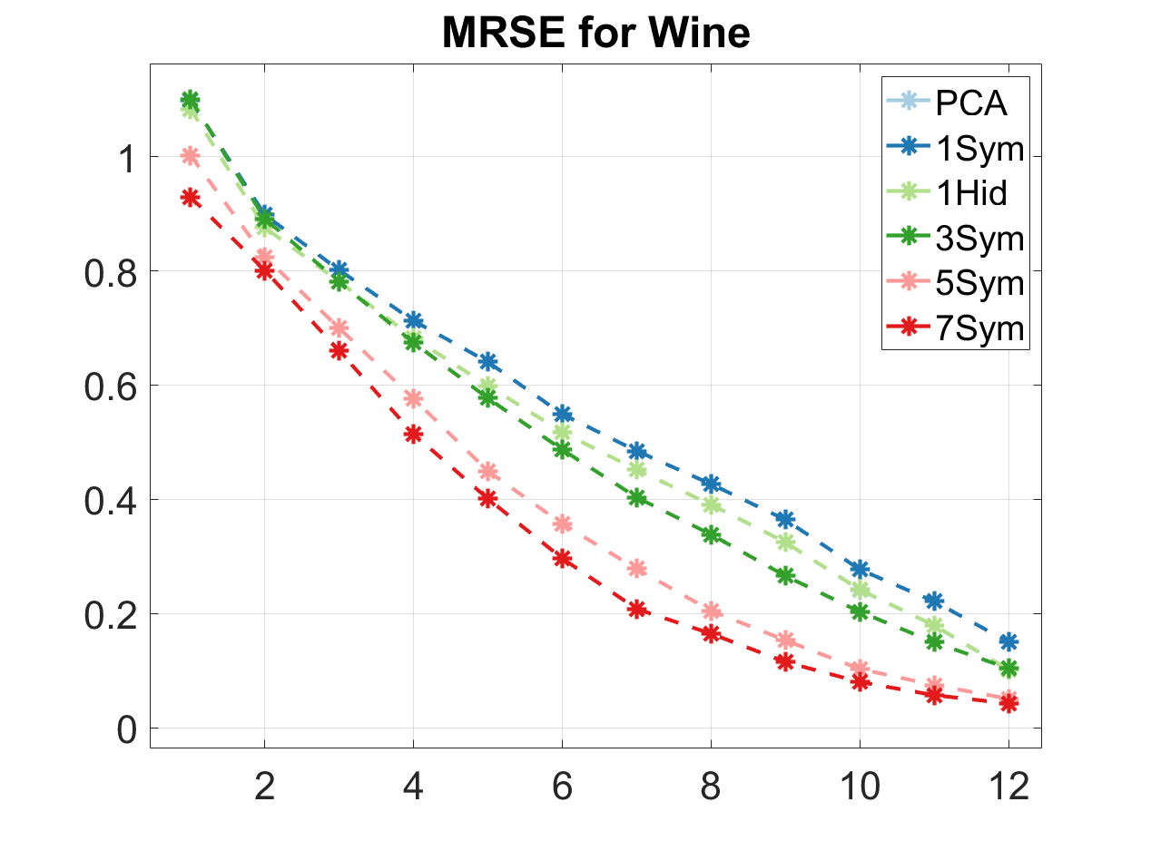
Interestingly, our experiments reveal that the intrinsic dimension can be identified by using only a shallow feedforward network as the nonlinear residual operator in the additive autoencoding model. This results from including the linear operator in the overall transformation and considering the unexplained residual in the original data dimension. This does not happen with the classical autoencoder (without linear term) or if an autoencoder would be used in the reduced dimension after the linear transformation. These phenomena, with the models and techniques fully specified in the subsequent sections, is illustrated in Fig. 1. Therefore, in addition to exploring the capabilities of revealing the intrinsic dimension we assess the advantages of applying deeper networks as nonlinear operators. Apparently, our results diversify views on the general superiority of deeper network architectures. They are also linked to the existing challenges that researchers need to address with deep learning techniques (Chen & Zhao 2018, Lathuilière et al. 2020, Ghods & Cook 2021).


1.1 On Autoencoders
Feedforward autoencoders have a versatile history, beginning from (Cottrell 1985, Bourlard & Kamp 1988). Their development as part of the evolution from shallow network models into deep learning techniques with various network architectures has been depicted in numerous large and comprehensive reviews (Schmidhuber 2015, LeCun et al. 2015, Jordan & Mitchell 2015). Therefore, we only provide a brief summary of these techniques below.
Deep feedforward autoencoding was highly influenced by the seminal work of Hinton & Salakhutdinov 2006. The work emphasized the importance of pretraining and the usability of stacking (i.e., layer-by-layer construction of the deeper architecture). Such techniques, by directing the determination of weights to a potential region of the search space, particularly alleviate the vanishing gradient problem (see (Schmidhuber 2015, Section 5.9) and references therein).
As summarized—for example, by (Liu et al. 2017), many architectures and training variants for deep autoencoders (AE) have been proposed over the years:
- •
Denoising AEs (DAE) in which noise (see (Ho et al. 2010)) is added into the training data (Vincent et al. 2010, Chen et al. 2015, Ismail Fawaz et al. 2019, Probst & Rothlauf 2020, Ma et al. 2020).
- •
Sparse AEs (SAE) in which the number of active, non-,zero weights is minimized (Filzmoser et al. 2012) (see also (Schmidhuber 2015, Section 5.6.4)).
- •
Contractive AEs (CAE) in which the reconstruction phase is penalized (Diallo et al. 2021).
- •
Separable AEs (SAE) in which two separate deep autoencoders are applied to model signal and noise spectra (Sun et al. 2015) (cf. Siamese neural networks that do the opposite and use shared weights (Ahrabian & BabaAli 2019)).
- •
Graph AEs (GAE) in which graphs, or their nodes, are encoded into latent representations and back (Wu et al. 2021, Hou et al. 2022, Yoo et al. 2022).
- •
Variational AEs (VAE) which are deep generative models that utilize Bayesian networks in learning probability distribution of data for encoding and decoding (Dai et al. 2018, Burkhardt & Kramer 2019, Zhao et al. 2021, Takahashi et al. 2022).
- •
Regularized AEs (RAE) in which the suppression of the derivatives of the encoder and regularization function orthogonal to the manifold provide local characterization of data-generation density (Alain & Bengio 2014).
- •
Multi-modal AEs can handle and unify the processing of different data modalities (Janakarajan et al. 2022).
- •
Other AEs typically integrate concepts and techniques from relevant areas, for instance, autoencoder bottlenecks (AE-BN) that are based on Deep Belief Networks (Sainath et al. 2012) and rough autoencoders (RAE) where rough set based neurons are used in the layers (Khodayar et al. 2017).
A wide variety of tasks and domains has been and can be addressed with autoencoders. AEs are typically used in numerous application domains in scenarios where transfer learning can be utilized—for example, in speech processing (Deng et al. 2017), time series prediction (Sun et al. 2018), fault diagnostics (Sun et al. 2019), and machine vision (Kim et al. 2020). In addition, interesting unsupervised hybrids are provided—for example, by clustering techniques that incorporate AEs for feature transformation (Min et al. 2018, McConville et al. 2021) and unsupervised AE-based hashing methods that can be used for large-scale information retrieval (Zhang & Qian 2021). Further, AEs have been used for the estimation of data distribution (Khajenezhad et al. 2020). Use of a variational AE for joint estimation of a normal latent data distribution and the corresponding contributing dimensions has been addressed in (Ikeda et al. 2018). Yet another use case of autoencoders is outlier detection, which might need statistically robust first-order fitting techniques instead of second-order least-squares (Gao et al. 2020, Kärkkäinen & Heikkola 2004). Data imputation has been realized using a shallow autoencoder in (Narayanan et al. 2002) and, more recently, using deep autoencoders mainly for spatio-temporal data in (Tran et al. 2017, Abiri et al. 2019, Zhao et al. 2020, Li et al. 2020, Sangeetha & Kumaran 2020, Ryu et al. 2020).
1.2 Contributions and contents
The main contribution of the paper is the derivation and evaluation of the additive autoencoding model. We provide an experimental confirmation of the new autoencoder’s ability to reveal the intrinsic dimension and study the effect of model depth. Based on the similar residual idea than with the model, we also depict a simple layerwise pretraining technique. With minor role, mostly covered in the Supplementary Information (SI), we also discuss and provide an experimental illustration of the difficulties of currently popular deep learning techniques in realizing the potential of deep network models. Overall, our results suggest that current and upcoming applications in deep learning could be improved by using an explicit separation of the linear and nonlinear aspects of the data-driven model. Moreover, it might be helpful to apply more accurate training techniques.
The remainder of the paper is organized in the following manner: In Section 2, we discuss the formalization of the proposed method as a whole. In Section 3, we describe the computational experiments and summarize the main findings. In Section 4, we provide the overall conclusions and discussion. In the SI, we provide more background and preliminary material and, especially, report the computational experiments as a whole. Main findings solely covered on SI confirm the quality of the implementation of the methods and especially indicate that different autoencoder models, as depicted in the previous section, could be used for the nonlinear residual estimation.
2 Methods
In this section, we describe the methods used here as part of the autoencoding approach. In the following account, we assume that a training set of observations , where , is given.
2.1 The autoencoding model
In mathematical modelling, linear and nonlinear models are typically treated separately (Bellomo & Preziosi 1994). Following Kärkkäinen 2022, according to Taylor’s formula, in the neighborhood of a point , the value of a sufficiently smooth real-valued function can be approximated as
where denotes the gradient vector and the Hessian matrix at . According to (Dennis Jr. & Schnabel 1996, Lemma 4.1.5), there exists (a line segment connecting the two points), such that
| (1) |
This formula yields the sufficient condition of to be the local minimizer of a convex (whose Hessian is positive semidefinite) (Nocedal & Wright 2006, Theorem 2.2): . However, another interpretation of the formula above is that we can locally approximate the value of a smooth function as a sum of its bias (i.e., constant level), a linear term, and a nonlinear higher-order residual operator. This observation is the starting point for proposing an autoencoder that has exactly such an additive structure.
The bias estimation simply involves the elimination of its effect through normalization by subtracting the data mean and scaling each feature separately into the same range with the scaling factor . Thus, we combine the mean component from z-scoring and the scaling component from min-max scaling. The reason for this is that the unit value of the standard deviation in z-scoring does not guarantee equal ranges, and min-max scaling into does not preserve the zero mean.
In the second phase, we estimate the linear behavior of the normalized data by using the classical principal component transformation (Bishop 1995). For a zero-mean vector , the transformation to a smaller-dimensional space spanned by principal components (PCs) is given by , where consists of the most significant (as measured by the sizes of the corresponding eigenvalues) eigenvectors of the covariance matrix. Thus, because of the orthonormality of , the unexplained residual variance of the PC coordinates (i.e., the linear trend in ) in the original space (see SI, Section 7) can be estimated in the following manner:
| (2) |
This transformation is referred to as PCA. With erroneous data or data with missing values, mean and classical PCA can be replaced with their statistically robust counterparts (Kärkkäinen & Saarela 2015).
In the third, nonlinear phase, we apply the classical fully connected feedforward autoencoder to the residual vectors in (2). As anticipated by the scaling, the activation function is used. This ensures the smoothness of the entire transformation and the optimization problem of determining the weights. The currently popular rectified linear units are nondifferentiable (Kärkkäinen & Heikkola 2004) and, therefore, are not theoretically compatible with the gradient-based methods (Goodfellow et al. 2016, Section 6.3.1). The importance of differentiability was also noted in (Ghods & Cook 2021).
The formalism introduced by Kärkkäinen 2002 is used for the compact derivation of the optimality conditions. By representing the layerwise activation using diagonal function-matrix , where , the output of a feedforward network with layers and linear activation on the final layer reads as
| (3) |
where for an input vector , and . To allow the formal adjoint transformation to be used as the decoder, we assume that is even and that the bias nodes are not included in (3). The dimensions of the weight matrices are then given by . In the autoencoding context, and define the sizes (the number of neurons) of the hidden layers with the squeezing dimension .
To determine the weights in (3), we minimize the regularized mean least-squares cost function of the form
| (4) |
where denotes the Frobenius norm and the number of rows of . Let be fixed to 1e-6 throughout; to simplify the notations, we define . The underlying idea in (4) is to average in both terms: in the first, the data fidelity (least-squares error, LSE) term, and in the second, the regularization term. Averaging the first term with implies that the term scales automatically by the size of the data subset, for instance, in minibatching, thereby providing an approximation of the entire LSE on a comparable scale. In the second term, because is fixed, the inverse scaling constant balances the effect of the regularization compared to the data fidelity for networks with a different number of layers of different sizes. Because (4) will be minimized with local optimizers, we simply use the initial guesses of the weight values in the second term to improve the local coercivity of (4) and to restrict the magnitude of the weights, thereby attempting to improve generalization (Gouk et al. 2021). Because of the residual approximation, the random initialization of the weight matrices is generated from the uniform distribution . s
The gradient matrices for (4) are of the following form (see Kärkkäinen 2002):
| (5) |
where the layerwise error backpropagation reads as
| (6) | |||||
| (7) |
The use of different weights in the encoding—that is, in the transformation until layer —and decoding, from layer to , implies more flexibility in the residual autoencoder but also rougly doubles the amount of weights to be determined. Therefore, it is common to use the formal adjoint of the encoder as the decoder. Then, it is easy to see that the layerwise optimality conditions for read as
| (8) |
where . For convenience, we define —that is, the number of layers to be optimized with the symmetric models.
We note that when the layerwise formulae above are used with vector-based optimizers, we always need to reshape operations to toggle between the weight matrices and a column vector of all weights.
Remark 1
Let us briefly summarize the use of the additive autoencoder for an unseen dataset after it has been estimated (and the corresponding data structures have been stored) for the training data through the three phases. First, data is normalized through mean subtraction and feature scaling into the same range . Then, residuals according to formula (2) are computed and this residual data is fed to the feedforward autoencoder. Again due to (2), the reduced, -dimensional representation of new data is obtained as a sum of its PC projection and the output of the autoencoder’s squeezing layer. Formula (2) shows that the explicit formation of the residual data between linear and nonlinear representations can be replaced by setting and using this as the first transformation layer of the autoencoder for the normalized, unseen data.
2.2 Layerwise pretraining

The core idea of the proposed autoencoding model—additive combination of operators of different complexity—can be applied in the layerwise pretraining, that is, stacking of the nonlinear autoencoding part as well. We propose to use an identical network structure and learning paradigm for this purpose differently from, e.g., (Hinton & Salakhutdinov 2006). A similar idea appears with the deep residual networks (ResNets) in He et al. 2016, where consecutive residuals are stacked together using layer skips—for example, over two or three layers with batch normalization. Moreover, in ResNets, the layer skips can introduce additional weight matrices to the deep network model. However, the layer-by-layer pretraining of the symmetric autoencoder, from the heads toward the inner layers, can be simply performed directly.
The approach is illustrated in Fig. 2. For three hidden layers with two unknown weight matrices, and , we first estimate with the given data . Then, the output data of the estimated layer are used as the training data (the input and the desired output) for the second layer . Thereafter, the entire network is fine-tuned by optimizing over both weight matrices. The process from the heads to the inner layers is naturally enlarged for a larger number of hidden layers. We could then also apply partial fine-tuning—for example, to fine-tune the three hidden layers during the process of constructing a five-hidden-layer network. However, according to our tests and similar to Hinton & Salakhutdinov 2006, the layerwise pretraining suffices before fine-tuning the entire network. A special case of utilizing a simpler structure is the one-hidden-layer case: The symmetric model 1Sym with one weight matrix if first optimizer to obtain and then used in the form as the initial guess for optimizing the nonsymmetric model 1Hid with two weight matrices. Again such an approach could be generalized to multiple hidden-layer case for the nonsymmetric, deep autoencoding model.
Remark 2
As stated in the introduction, stacking attempts to mitigate the vanishing gradient problem, which may prevent the adaptation of the weights in deeper layers. We assessed the possibility of such a phenomenon by studying the relative changes in the weight matrix norms while fine-tuning the symmetric autoencoders with 3–7 layers (3Sym, 5Sym, and 7Sym; see Section 3). The subscripts ’0’ and ’’ refer to the initial and final weight matrix values, respectively. This study revealed that the relative changes in the weights in the deeper layers were not on a smaller numerical scale compared to the other layers. Apparently, the double role of the layers in the symmetric models as part of the encoder and the decoder, with the corresponding effect on the gradient as seen in formula (8), is also helpful in avoiding a vanishing gradient.
2.3 Determination of intrinsic dimension
The basic procedure to determine the intrinsic dimension is to gradually increase the size of the squeezing layer and to seek a small value of the reconstruction error measuring autoencoding error, with a knee point (Thorndike 1953) indicating that the level of nondeterministic residual noise has been reached in autoencoding. Instead of the usual root mean squared error (RMSE), we apply the mean root squared error (MRSE) to compute the autoencoding error:
| (9) |
where is assumed to be normalized and denotes the application of the autoencoder. This choice was made because in Kärkkäinen 2014, MRSE correlated better with the independent validation error. In practice, the difference between the RMSE and the MRSE is only the scaling factor, vs. . After the linear PC trend estimation, the MRSE is obtained by using (9) for the residual data defined in formula (2). Note that the reconstruction error is a strict error measure and its use requires higher accuracy from autoencoding compared to other measures: with the Wine dataset in Fig. 1, the linear PCA needs all dimensions of the rotated coordinate axis for the reconstruction whereas already 10 principal components out of 13 would explain over 96% of the data variance.
An example of determining the intrinsic dimension of the Glass dataset (see the next section) is presented in Fig. 3. In the figure, the -axis “SqDim” presents the squeezing dimension and the -axis on the left the “MRSE” and on the right its change “(MRSE)” (i.e., backward difference) for the symmetric model with one hidden dimension (1Sym) and the corresponding nonsymmetric model 1Hid. The intrinsic dimension of data is detected by first locating a sufficiently small change in the autoencoding error (the right plot). For this purpose, a user-defined threshold = 4e-3 is applied. The detected dimension 5 on the left, marked with a circle, is the dimension below the threshold on the right minus one. The intrinsic dimension 5 is also characterized by a clear knee point in the MRSE behavior.


3 Results
The main focus of the computational experiments, which are fully reported in the Supplementary Information (SI), was to investigate the ability of the proposed additive autoencoder model to represent a dataset in a lower-dimensional space. Therefore, we confined ourselves to the use of Matlab as the platform (mimicking the experiments in Hinton & Salakhutdinov 2006) to have full control over the realization of the methods in order to study the effects of different parameters and configurations. Reference implementation of the proposed method and its basic testing is available in GitHub11 1 https://github.com/TommiKark/AdditiveAutoencoder.
We apply and compare the following set of techniques to approximate the nonlinear residual of the autoencoder, after normalization and identification of the linear trend: 1Hid (model with one hidden layer and separate weight matrices for the encoder and the decoder), 1Sym (symmetric model with one hidden layer and a shared weight matrix), 3Sym (three-hidden-layer symmetric model with two shared weight matrices), 5Sym, and 7Sym. To systematically increase the flexibility and the approximation capability of the deeper models, the sizes of the layers for are given below, where is the size of the squeezing layer:
-
3Sym: – – ,
-
5Sym: – – – ,
-
7Sym: – – – – .
Note that for the size of the second layer and, therefore, the dimension of the first intermediate representation, is larger than the input dimension for all these models.
3.1 Identification of the intrinsic dimension
The first purpose of the experiments was to search for the intrinsic dimension of a dataset via autoencoding. This was done using the shallow models 1Sym and 1Hid. The optimization settings and visualization of all results are given in the online SM.
The experiments were carried out for two groups of datasets, one with small-dimension data (less than 100 features) and the other with large-dimension data (up to 1024 features). The datasets were obtained from the UCI repository (Dua & Graff 2017), except the FashMNIST, which was downloaded from GitHub22 2 https://github.com/zalandoresearch/fashion-mnist. For most of the datasets, only the training data was used; however, with Madelon, the given training, testing, and validation datasets were combined. The datasets do not contain missing values. The constant features were identified and eliminated according to whether the difference between the maximum and minimum values of a feature was less than , where denotes machine epsilon (this is classically used numerical proxy of zero, see (Dennis Jr. & Schnabel 1996, p. 12)). Because of this preprocessing, the number of features in Tables 1 and 2 is not necessarily the same as that in the UCI repository.
| Dataset | ID | Red | MRSE | FeatProf (%) | ||
|---|---|---|---|---|---|---|
| Glass | 214 | 10 | 5 | 0.50 | 1.3e-3 | 10-40-50-0 |
| Wine | 178 | 13 | 7 | 0.54 | 1.2e-3 | 0-46-54-0 |
| Letter | 20 000 | 16 | 8 | 0.50 | 9.4e-4 | 0-100-0-0 |
| SML2010 | 2 763 | 17 | 9 | 0.53 | 5.4e-4 | 0-12-18-71 |
| FrogMFCC | 7 195 | 22 | 11 | 0.50 | 1.1e-3 | 0-0-5-95 |
| SteelPlates | 1 941 | 27 | 11 | 0.41 | 4.3e-3 | 11-11-56-22 |
| BreastCancerW | 569 | 30 | 14 | 0.47 | 6.9e-3 | 0-0-100-0 |
| Ionosphere | 351 | 33 | 17 | 0.52 | 1.9e-3 | 3-0-97-0 |
| SatImage | 6 435 | 36 | 18 | 0.50 | 4.3e-4 | 0-75-25-0 |
| SuperCond | 21 263 | 82 | 37 | 0.45 | 1.1e-2 | 2-1-12-84 |
| COIL2000 | 5 822 | 85 | 35 | 0.41 | 2.8e-2 | 99-1-0-0 |
| Dataset | ID | Red | MRSE | FeatProf (%) | ||
|---|---|---|---|---|---|---|
| USPS | 9 298 | 256 | 130 | 0.51 | 2.9e-3 | 0-0-0-100 |
| BlogPosts | 52 397 | 277 | 130 | 0.47 | 3.9e-3 | 79-8-12-1 |
| CTSlices | 53 500 | 379 | 180 | 0.47 | 6.3e-2 | 8-4-10-78 |
| UJIIndoor | 19 937 | 473 | 200 | 0.42 | 7.0e-2 | 26-73-1-0 |
| Madelon | 4 400 | 500 | 250 | 0.50 | 7.9e-2 | 2-31-67-0 |
| HumActRec | 7 351 | 561 | 220 | 0.39 | 8.0e-2 | 0-2-0-98 |
| Isolet | 7 797 | 617 | 310 | 0.50 | 9.4e-3 | 1-6-14-80 |
| MNIST | 60 000 | 717 | 350 | 0.49 | 9.3e-3 | 9-14-77-0 |
| FashMNIST | 60 000 | 784 | 380 | 0.48 | 5.0e-2 | 0-2-98-0 |
| COIL100 | 7 200 | 1 024 | 560 | 0.55 | 6.4e-3 | 0-11-89-0 |
During the search, the squeezing dimension for the small-dimension datasets began from one and was incremented one by one up to . For the large-dimension cases, we began from 10 and used increments of until the maximum squeezing dimension was reached (cf. the “Red” values in Tables 1 and 2). The experiments were run with Matlab on a Laptop with 2.3GHz Intel i7 processor and 64 GB RAM and on a server with a Xeon E5-2690 v4 CPU and 384 GB of memory.
In Tables 1 and 2, we present the name of the dataset, the number of observations , the number of features , and the detected intrinsic dimension ID. The autoencoding error trajectories and thresholdings are illustrated for all datasets in the online SM. The detection threshold for small-dimension datasets was fixed to = 4e-3. The reduction rate ID for the intrinsic data dimension is reported in the Red column, and the autoencoding error of 1Hid for ID according to (9) is included in the MRSE column. There is no averaging over the data dimension in (9), so that for higher-dimension datasets this error is expected to remain larger. This was probably one of the reasons why, for large-dimension datasets, we needed to use two values of the threshold (based on visual inspection; see the zoomed illustrations in the SM): 3e-3 for USPS, BlogPosts, HumActRec, MNIST, and COIL100, and 3e-2 for the remaining five datasets.


For the analysis, we also included a depiction of how discrete or continuous the set of features for a dataset is. We categorized the features into four groups based on the number of unique values (UV) each feature has: C1 = {UV 10}, C2 = {10 UV 100}, C3 = {100 UV 1000}, and C4 = {1000 UV}. The FeatProf column in Tables 1 and 2 presents the proportions of C1–C4 in percentages.
Conclusions
Examples of the ID detection are given in Figs. 3 (Glass), 4 (Letter on the left, SuperCond on the right), 5 (MNIST), and 6 (FashMNIST on the left, COIL100 on the right). Identifications in the first two cases and for FashMNIST are characterized by clear knee-points in IDs. For SuperCond, with gradual decrease of the MRSE, determination of ID is based on the mutual threshold value = 4e-3 of small-dimension datasets. Also MNIST has such a behavior and the zoom in Fig. 5 (right) illustrates the detection decision with = 3e-3.
Overall, the intrinsic dimensions were successfully identified for all tested datasets. The use of a feedforward network to approximate the nonlinear residual notably decreased the autoencoding error of the linear PCA. The overall transformation summarizing the essential behavior of data roughly halved the original dimension: The mean reduction rate over the 21 datasets was 0.48.
The reduction rate was independent of the form of the features—that is, the best reduction rates for small-dimension datasets were obtained with the very categorical COIL2000 and primarily continuous SteelPlates datasets. However, the best reduction rate, 0.39, was obtained for HumActRec, which is characterized by a continuous feature profile. This indicates that we may obtain smaller reduction rates with more continuous sets of features.
3.2 Comparison of shallow and deep models
| 1Sym | 3Sym | 5Sym | 7Sym | |||||
|---|---|---|---|---|---|---|---|---|
| Dataset | mean | max (dim) | mean | max (dim) | mean | max (dim) | mean | max (dim) |
| Glass | 0.91 | 1.03 (2) | 0.91 | 1.10 (3) | 1.18 | 1.31 (3) | 1.15 | 1.40 (3) |
| Wine | 0.97 | 0.99 (1) | 1.07 | 1.22 (6) | 1.25 | 1.59 (6) | 1.36 | 1.75 (6) |
| Letter | 1.00 | 1.00 (1) | 1.03 | 1.06 (6) | 1.10 | 1.14 (6) | 1.11 | 1.15 (6) |
| SML2010 | 0.94 | 0.99 (1) | 0.95 | 1.07 (5) | 1.12 | 1.23 (3) | 1.15 | 1.32 (3) |
| FrogMFCCs | 0.99 | 1.00 (7) | 1.04 | 1.17 (8) | 1.10 | 1.23 (8) | 1.11 | 1.23 (8) |
| SteelPlates | 0.94 | 0.99 (4) | 0.94 | 1.09 (5) | 1.04 | 1.22 (5) | 1.04 | 1.27 (5) |
| BreastCancerW | 0.98 | 0.99 (11) | 1.10 | 1.29 (13) | 1.22 | 1.42 (12) | 1.24 | 1.41 (11) |
| Ionosphere | 0.91 | 0.97 (3) | 1.04 | 1.26 (15) | 1.74 | 3.19 (14) | 2.07 | 4.06 (15) |
| Satimage | 0.99 | 1.00 (10) | 1.02 | 1.07 (17) | 1.05 | 1.09 (17) | 1.06 | 1.12 (1) |
| SuperCond | 1.00 | 1.00 (30) | 1.10 | 1.18 (33) | 1.20 | 1.30 (29) | 1.23 | 1.34 (26) |
| COIL2000 | 0.99 | 1.02 (16) | 1.24 | 1.85 (32) | 1.49 | 2.89 (29) | 1.48 | 2.62 (30) |
| 1Sym | 3Sym | 5Sym | 7Sym | |||||
|---|---|---|---|---|---|---|---|---|
| Dataset | mean | max (dim) | mean | max (dim) | mean | max (dim) | mean | max (dim) |
| USPS | 0.99 | 1.00 (90) | 1.08 | 1.16 (90) | 1.13 | 1.21 (70) | 1.14 | 1.23 (60) |
| BlogPosts | 0.95 | 1.00 (110) | 1.18 | 1.39 (70) | 1.28 | 1.56 (80) | 1.23 | 1.53 (70) |
| CTSlices | 0.99 | 1.00 (170) | 1.17 | 1.51 (150) | 1.30 | 1.76 (150) | 1.32 | 1.74 (150) |
| UJIIndoor | 0.99 | 0.99 (60) | 1.69 | 2.46 (150) | 2.15 | 3.11 (130) | 2.24 | 3.51 (130) |
| Madelon | 0.97 | 1.00 (30) | 1.38 | 3.74 (240) | 2.29 | 5.77 (220) | 3.01 | 8.02 (220) |
| HumActRec | 0.99 | 1.00 (160) | 1.15 | 1.31 (160) | 1.22 | 1.40 (130) | 1.24 | 1.40 (130) |
| Isolet | 0.99 | 1.00 (290) | 1.22 | 2.16 (290) | 1.44 | 2.89 (270) | 1.55 | 2.65 (270) |
| MNIST | 0.99 | 1.00 (200) | 1.32 | 1.99 (260) | 1.42 | 2.20 (250) | 1.41 | 2.25 (240) |
| FashMNIST | 0.99 | 1.00 (320) | 1.15 | 1.63 (370) | 1.22 | 1.59 (350) | 1.23 | 1.53 (350) |
| COIL100 | 0.98 | 1.00 (310) | 2.18 | 11.19 (520) | 1.96 | 8.51 (530) | 1.79 | 2.63 (430) |
| COIL100-Min | 0.98 | 1.00 (310) | 1.75 | 8.05 (510) | 1.79 | 4.22 (510) | 1.87 | 2.63 (430) |


The second aim of the experiments was to examine whether deeper network structures and deep learning techniques (the network structure and optimization of the weights) can improve the identification of the intrinsic dimension and the data restoration ability of the additive autoencoder. This aim is pursued as follows: Here, we compare shallow and deep networks in cases where fine-tuning is performed using a classical optimization approach, i.e., using the L-BFGS optimizer with the complete dataset. In the SI, we report the results of using different minibatch-based approaches. Also detailed depictions of the parameter choices and visualization of the results for all datasets are included there.
In addition to visual assessment, we performed a quantitative comparison between the deep and shallow models. First, the MRSE values of all models were divided with the corresponding value of the 1Hid model’s error. This was done for the squeezing dimensions from the first until next to last of ID, to cover the essential search phase of the intrinsic dimension. To exemplify relative performance, if the MRSE value of a model divided by the 1Hid’s value for a particular squeezing dimension would be 0.5, then such a model would have half the error level and, conversely, twice the efficiency compared to 1Hid. Therefore, the model’s efficiency is defined as the reciprocal of relative performance.
The relative performances are illustrated in Figs. 7 and 8. Descriptive statistics of the efficiencies of symmetric models are given in Tables 3 and 4. In each cell there, both the mean efficiency and the maximal efficiency are provided. The latter includes, in parentheses, the squeezing dimension where it was encountered.
Conclusions
During the early phases of searching the intrinsic dimension, deep networks provide smaller autoecoding errors compared to the shallow models. However, as exemplified in Fig. 7 (left) and is evident from all illustrations in the SI, MRSE in ID is not better for deeper models compared to 1Hid. Therefore, the use of a deeper model would not change the ID values and, in fact, fluctuation of the error compared to 1Hid may hinder the detection of a knee-point and negatively affect the simple thresholding.
Usually, the mean efficiency of the two deepest models, 5Sym and 7Sym, is better than that of 1Sym or 3Sym, but for many datasets, there is only a slight improvement. Overall, the plots for the relative efficiencies between different symmetric models and the quantitative trends in the rows of Tables 3 and 4 include varying patterns. The mean efficiency is highest for UJIIndoor, Ionosphere, Madelon, and COIL100, where the last three datasets are characterized by high data dimension/number of observations, , ratio (0.09, 0.11, and 0.08, respectively). The following are the grand means of the mean efficiencies over all 21 datasets for the symmetric models: 1Sym 0.97, 3Sym 1.19, 5Sym 1.38, and 7Sym 1.44. This concludes that deeper models improve the reduction of the autoencoding error during the search of ID. However, the speed of improvement decreases as a function of the number of layers.
Actually, close to the intrinsic dimension, the benefits of deeper models may be completely lost. This is illustrated in Fig. 8 (right) and in Table 4 for COIL100 (see also, for example, plots of BlogPosts and MNIST in the SI). The reason for such a behavior with COIL100 is the value of ID, 560, which was obtained with the smaller threshold = 3e-3 for large-dimension datasets. Therefore, with COIL100, we also tested an alternative approach to the identification of ID, where we apply the same thresholding technique (and the same ) to the minimum autoencoding error of the all models. This error plot, the identified ID = 520 (for which the reduction rate would be 0.51), and the corresponding reduced set of relative efficiencies are illustrated in Figure 9. The summary of the efficiencies for this modified way to identify ID are given in the last line “COIL100-Min” in Table 4. It can be concluded that for the largest dimensional dataset COIL100, the use of the minimum autoencoding error of the models yielded more reasonable results.


We used a fixed pattern for the sizes of the hidden layers in deeper models: 2-3-4 times the squeezing dimension for 7Sym, the first and last of these coefficients for 5Sym, and the first one for 3Sym. As reported in Section 3.1, the mean reduction rate over the 21 datasets was close to 0.5. Therefore, one may wonder whether this behavior is due to the fact that from this case onwards all the hidden dimensions are larger than the number of features so that a kind of nonlinear kernel trick occurs. In other words, would a different pattern of the hidden dimensions change the results and conclusions here? This consideration was tested by considering a 3-5-7 pattern providing much more flexibility for the nonlinear operator compared to the used pattern. These tests are not reported as a whole, because the clearly identified trend of the results is readily exemplified in Fig. 10: Increase of the sizes of the hidden layers slightly improve the reduction rate during early phase of the search but does not change the value of the ID.


3.3 Generalization of the autoencoder
In the last experiments, we demonstrate and evaluate the generalization of the additive 5Sym autoencoder. Search over squeezing dimensions is performed in a similar manner as that done in Section 3.2. We apply a small sample of datasets, for which a separate validation data was given in the UCI repository. More precisely, we use Letter (size of training data , size of validation data , i.e., 80%–20% portions with respect to the entire data; number of nonconstant featureas ), UJIIndoor ( 95%–5% portions; ), HumActRecog ( 71%–29% portions; ), and MNIST ( 86%–14% portions; ). Note that because all data are used as is, we have no information or guarantees on how well the data distributions in the training and validation sets actually match each other.


As anticipated, both training-validation portions and the data dimension affected the generalization results. For Letter, with 80%-20% division between training-validation sizes and small number of features, we witnessed a perfect match between the training and validation MRSE values. The same held true for MNIST, which is illustrated in Fig. 11 (right). The largest discrepancy between the training and validation errors, depicted in Figure 11 (left), was obtained for UJIIndoor, which has the most deviating 95%-5% portions with almost 500 features. This dataset also had one of the largest efficiencies (i.e., reduction potential) in Table 4. HumActRec was somewhere in the middle in its behavior, with clearly visible deviation. Because of the data portions (70%-30%), the difference raises doubts regarding the quality of the validation set. Note that these considerations provide examples of the possibilities of autoencoders to assess the quality of data.
The visual inspection was augmented by computing the correlation coefficient between the MRSE values in the training and validation sets. The following values confirmed the conclusions of the visual inspection: Letter 1.0000, UJIIndoor 0.9766, HumActRecog 0.9939, and MNIST 0.9999. Finally, an important observation from Fig. 11 is that when the squeezing dimension is increased up to the intrinsic dimension, then the validation error tends to the same error level than the training error. Therefore, the additive autoencoder determined using the training data was always able to explain the variability of the validation data with a compatible accuracy.
4 Conclusions
This study illustrated a case where all main concerns with feedforward mappings summarized in (Hornik et al. 1989, p. 363) were solved: learning was successful, the size and the number of hidden layers were identified, and the deterministic relationship within a dataset was found. Similar to Hinton & Salakhutdinov 2006, stacking was found to be an essential building block for estimating the weights of deep autoencoders. However, the pretraining face was conceptually (the structure and optimization of the weights) one-to-one with the corresponding part of the final, fine-tuned autoencoder. This was different from deep residual networks (He et al. 2016), where layer skips over multiple layers with batch normalization were applied. The other main ingredients of the proposed autoencoder were an automatically scalable cost function with compact layerwise weight calculus and a simple heuristic for determining the intrinsic data dimension. Intrinsic dimensions for all tested datasets with a low autoencoding error were revealed. A similar autoencoding error, and the corresponding intrinsic dimension, was obtained independently on the depth of the network.
One clear advantage of the proposed methodology is the lack of meta-level parameters (e.g., number and form of layers, selection of activation function, detection of the learning rate) that are usually tuned or grid-searched when DNNs are trained. The only parameter that may need adjustment based on visual assessment is —that is, the threshold for identifying the hidden dimension. Moreover, because of the observed smoothly decreasing behavior of the autoencoding error, the intrinsic dimension could be searched for more efficiently than just incrementally: One could attempt to utilize one-dimensional optimization techniques like a golden-section search and/or polynomial and spline interpolation to more quickly identify the beginning of the error plateau.
These results challenge the common beliefs and currently popular traditions with deep learning techniques. The experiments summarized here and given in the SI suggest that many existing deep learning results could be improved by using a clear separation of linear and nonlinear data-driven models. Also use of more accurate optimization techniques to determine the weights of such models may be advantageous.
We can use the additive transformation to the intrinsic dimension as a pretrained part for transfer learning with any prediction or classification model (Ghods & Cook 2021). It would be interesting to test in the future whether one should use this as is or would a transformation into a smaller squeezing dimension than the intrinsic one generalize better in prediction and classification tasks? Another detectable dimensions of the squeezing layer worth investigating, as illustrated in the relative MRSE plots (see also the SI) and in Tables 3 and 4, could be the one with the largest nonlinear gain—that is, with the maximum difference between the PCA error and the autoencoder error or between the shallow and deep results. Moreover, we used global techniques in every part of the autoencoder. The technique might benefit from encoding locally estimated behavior—for example, using convolutional layers for local-level estimation (LeCun et al. 1990). Similarly, other linear transformation techniques and modifications of PCA might provide better performance (Burges et al. 2010, Song et al. 2018, Vogelstein et al. 2021), although in the proposed form, we also need the inverse of the linear mapping to be able to estimate the residual error in the original vector space.
Supplementary information and availability of data and implementations
Further information concerning this manuscript is given in the public git-repository:
https://github.com/TommiKark/AdditiveAutoencoder.
There, complementary background material and some additional methodological comparisons are given in a separate Supplementary Information document. Especially, full coverage of all the results and illustrations of the computational experiments are documented there. All data or links for downloading data from public repositories used in the experiments are provided. The reference implementation of the proposed methods are also included.
Acknowledgments
This work was supported by the Academy of Finland from the project 351579 (MLNovCat).
References
- (1)
- Abiri et al. (2019) Abiri, N., Linse, B., Edén, P. & Ohlsson, M. (2019), ‘Establishing strong imputation performance of a denoising autoencoder in a wide range of missing data problems’, Neurocomputing 365, 137–146.
- Ahrabian & BabaAli (2019) Ahrabian, K. & BabaAli, B. (2019), ‘Usage of autoencoders and siamese networks for online handwritten signature verification’, Neural Computing and Applications 31(12), 9321–9334.
- Alain & Bengio (2014) Alain, G. & Bengio, Y. (2014), ‘What regularized auto-encoders learn from the data-generating distribution’, The Journal of Machine Learning Research 15(1), 3563–3593.
- Bahadur & Paffenroth (2019) Bahadur, N. & Paffenroth, R. (2019), ‘Dimension estimation using autoencoders’, arXiv preprint arXiv:1909.10702 .
- Bahadur & Paffenroth (2020) Bahadur, N. & Paffenroth, R. (2020), Dimension estimation using autoencoders with applications to financial market analysis, in ‘2020 19th IEEE International Conference on Machine Learning and Applications (ICMLA)’, IEEE, pp. 527–534.
- Bellomo & Preziosi (1994) Bellomo, N. & Preziosi, L. (1994), Modelling mathematical methods and scientific computation, Vol. 1, CRC press.
- Bishop (1995) Bishop, C. M. (1995), Neural Networks for Pattern Recognition, Oxford University Press.
- Bourlard & Kamp (1988) Bourlard, H. & Kamp, Y. (1988), ‘Auto-association by multilayer perceptrons and singular value decomposition’, Biological cybernetics 59(4), 291–294.
- Burges et al. (2010) Burges, C. J. et al. (2010), ‘Dimension reduction: A guided tour’, Foundations and Trends® in Machine Learning 2(4), 275–365.
- Burkhardt & Kramer (2019) Burkhardt, S. & Kramer, S. (2019), ‘Decoupling sparsity and smoothness in the dirichlet variational autoencoder topic model’, Journal of Machine Learning Research 20(131), 1–27.
- Camastra (2003) Camastra, F. (2003), ‘Data dimensionality estimation methods: a survey’, Pattern recognition 36(12), 2945–2954.
- Camastra & Staiano (2016) Camastra, F. & Staiano, A. (2016), ‘Intrinsic dimension estimation: Advances and open problems’, Information Sciences 328, 26–41.
- Chen et al. (2015) Chen, M., Weinberger, K. Q., Xu, Z. & Sha, F. (2015), ‘Marginalizing stacked linear denoising autoencoders’, The Journal of Machine Learning Research 16(1), 3849–3875.
- Chen & Zhao (2018) Chen, S. & Zhao, Q. (2018), ‘Shallowing deep networks: Layer-wise pruning based on feature representations’, IEEE transactions on pattern analysis and machine intelligence 41(12), 3048–3056.
- Cottrell (1985) Cottrell, G. W. (1985), Learning internal representations from gray-scale images: An example of extensional programming, in ‘Proceedings Ninth Annual Conference of the Cognitive Science Society, Irvine, CA.’, pp. 462–473.
- Dai et al. (2018) Dai, B., Wang, Y., Aston, J., Hua, G. & Wipf, D. (2018), ‘Connections with robust PCA and the role of emergent sparsity in variational autoencoder models’, The Journal of Machine Learning Research 19(1), 1573–1614.
- Deng et al. (2017) Deng, J., Frühholz, S., Zhang, Z. & Schuller, B. (2017), ‘Recognizing emotions from whispered speech based on acoustic feature transfer learning’, IEEE Access 5, 5235–5246.
- Dennis Jr. & Schnabel (1996) Dennis Jr., J. E. & Schnabel, R. B. (1996), Numerical Methods for Unconstrained Optimization and Nonlinear Equations, Vol. 16, Siam.
- Diallo et al. (2021) Diallo, B., Hu, J., Li, T., Khan, G. A., Liang, X. & Zhao, Y. (2021), ‘Deep embedding clustering based on contractive autoencoder’, Neurocomputing 433, 96–107.
- Dua & Graff (2017)
Dua, D. & Graff, C. (2017), ‘UCI
Machine Learning Repository’.
http://archive.ics.uci.edu/ml - Facco et al. (2017) Facco, E., d’Errico, M., Rodriguez, A. & Laio, A. (2017), ‘Estimating the intrinsic dimension of datasets by a minimal neighborhood information’, Scientific reports 7(1), 1–8.
- Filzmoser et al. (2012) Filzmoser, P., Gschwandtner, M. & Todorov, V. (2012), ‘Review of sparse methods in regression and classification with application to chemometrics’, Journal of Chemometrics 26(3-4), 42–51.
- Fukunaga (1982) Fukunaga, K. (1982), ‘Intrinsic dimensionality extraction’, Handbook of statistics 2, 347–360.
- Fukunaga & Olsen (1971) Fukunaga, K. & Olsen, D. R. (1971), ‘An algorithm for finding intrinsic dimensionality of data’, IEEE Transactions on Computers 100(2), 176–183.
- Gao et al. (2020) Gao, Y., Shi, B., Dong, B., Chen, Y., Mi, L., Huang, Z. & Shi, Y. (2020), RVAE-ABFA: robust anomaly detection for highdimensional data using variational autoencoder, in ‘2020 IEEE 44th Annual Computers, Software, and Applications Conference (COMPSAC)’, IEEE, pp. 334–339.
- Ghods & Cook (2021) Ghods, A. & Cook, D. J. (2021), ‘A survey of deep network techniques all classifiers can adopt’, Data mining and knowledge discovery 35(1), 46–87.
- Goodfellow et al. (2016) Goodfellow, I., Bengio, Y. & Courville, A. (2016), Deep Learning, MIT Press.
- Gouk et al. (2021) Gouk, H., Frank, E., Pfahringer, B. & Cree, M. J. (2021), ‘Regularisation of neural networks by enforcing lipschitz continuity’, Machine Learning 110(2), 393–416.
- He et al. (2016) He, K., Zhang, X., Ren, S. & Sun, J. (2016), Deep residual learning for image recognition, in ‘Proceedings of the IEEE Conference on Computer Vision and Pattern Recognition’, pp. 770–778.
- Hinton & Salakhutdinov (2006) Hinton, G. E. & Salakhutdinov, R. R. (2006), ‘Reducing the dimensionality of data with neural networks’, Science 313(5786), 504–507.
- Ho et al. (2010) Ho, K., Leung, C.-S. & Sum, J. (2010), ‘Objective functions of online weight noise injection training algorithms for MLPs’, IEEE transactions on neural networks 22(2), 317–323.
- Hornik et al. (1989) Hornik, K., Stinchcombe, M. & White, H. (1989), ‘Multilayer feedforward networks are universal approximators.’, Neural Networks 2(5), 359–366.
- Hou et al. (2022) Hou, Z., Liu, X., Dong, Y., Wang, C., Tang, J. et al. (2022), Graphmae: Self-supervised masked graph autoencoders, in ‘Proceedings o the 28th ACM SIGKDD Conference on Knowledge Discovery and Data Mining’, pp. 594–604.
- Ikeda et al. (2018) Ikeda, Y., Tajiri, K., Nakano, Y., Watanabe, K. & Ishibashi, K. (2018), ‘Estimation of dimensions contributing to detected anomalies with variational autoencoders’, arXiv preprint arXiv:1811.04576 .
- Ismail Fawaz et al. (2019) Ismail Fawaz, H., Forestier, G., Weber, J., Idoumghar, L. & Muller, P.-A. (2019), ‘Deep learning for time series classification: a review’, Data mining and knowledge discovery 33(4), 917–963.
- Janakarajan et al. (2022) Janakarajan, N., Born, J. & Manica, M. (2022), A fully differentiable set autoencoder, in ‘Proceedings of the 28th ACM SIGKDD Conference on Knowledge Discovery and Data Mining’, pp. 3061–3071.
- Jolliffe (2002) Jolliffe, I. (2002), Principal Component Analysis, 2 edn, Springer Verlag.
- Jordan & Mitchell (2015) Jordan, M. I. & Mitchell, T. M. (2015), ‘Machine learning: Trends, perspectives, and prospects’, Science 349(6245), 255–260.
- Kärkkäinen (2002) Kärkkäinen, T. (2002), ‘MLP in layer-wise form with applications to weight decay’, Neural Computation 14(6), 1451–1480.
- Kärkkäinen (2014) Kärkkäinen, T. (2014), On cross-validation for MLP model evaluation, in ‘Joint IAPR International Workshops on Statistical Techniques in Pattern Recognition (SPR) and Structural and Syntactic Pattern Recognition (SSPR)’, Springer, pp. 291–300.
- Kärkkäinen (2022) Kärkkäinen, T. (2022), On the role of Taylor’s formula in machine learning, in ‘Impact of scientific computing on science and society’, Springer Nature. (18 pages, to appear).
- Kärkkäinen & Heikkola (2004) Kärkkäinen, T. & Heikkola, E. (2004), ‘Robust formulations for training multilayer perceptrons’, Neural Computation 16(4), 837–862.
- Kärkkäinen & Rasku (2020) Kärkkäinen, T. & Rasku, J. (2020), Application of a knowledge discovery process to study instances of capacitated vehicle routing problems, in ‘Computation and Big Data for Transport, Chapter 6’, Computational Methods in Applied Sciences, Springer-Verlag, pp. 1–25.
- Kärkkäinen & Saarela (2015) Kärkkäinen, T. & Saarela, M. (2015), Robust principal component analysis of data with missing values, in ‘International Workshop on Machine Learning and Data Mining in Pattern Recognition’, Springer, pp. 140–154.
- Khajenezhad et al. (2020) Khajenezhad, A., Madani, H. & Beigy, H. (2020), ‘Masked autoencoder for distribution estimation on small structured data sets’, IEEE Transactions on Neural Networks and Learning Systems . Early Access, to appear.
- Khodayar et al. (2017) Khodayar, M., Kaynak, O. & Khodayar, M. E. (2017), ‘Rough deep neural architecture for short-term wind speed forecasting’, IEEE Transactions on Industrial Informatics 13(6), 2770–2779.
- Kim et al. (2020) Kim, S., Noh, Y.-K. & Park, F. C. (2020), ‘Efficient neural network compression via transfer learning for machine vision inspection’, Neurocomputing 413, 294–304.
- Lathuilière et al. (2020) Lathuilière, S., Mesejo, P., Alameda-Pineda, X. & Horaud, R. (2020), ‘A comprehensive analysis of deep regression’, IEEE transactions on pattern analysis and machine intelligence 42(9), 2065–2081.
- LeCun et al. (2015) LeCun, Y., Bengio, Y. & Hinton, G. (2015), ‘Deep learning’, Nature 521(7553), 436–444.
- LeCun et al. (1990) LeCun, Y., Boser, B. E., Denker, J. S., Henderson, D., Howard, R. E., Hubbard, W. E. & Jackel, L. D. (1990), Handwritten digit recognition with a back-propagation network, in ‘Advances in Neural Information Processing Systems’, pp. 396–404.
- Lee & Verleysen (2007) Lee, J. A. & Verleysen, M. (2007), Nonlinear dimensionality reduction, Springer Science & Business Media.
- Li et al. (2020) Li, L., Franklin, M., Girguis, M., Lurmann, F., Wu, J., Pavlovic, N., Breton, C., Gilliland, F. & Habre, R. (2020), ‘Spatiotemporal imputation of MAIAC AOD using deep learning with downscaling’, Remote sensing of environment 237, 111584.
- Liu et al. (2017) Liu, W., Wang, Z., Liu, X., Zeng, N., Liu, Y. & Alsaadi, F. E. (2017), ‘A survey of deep neural network architectures and their applications’, Neurocomputing 234, 11–26.
- Ma et al. (2020) Ma, Q., Lee, W.-C., Fu, T.-Y., Gu, Y. & Yu, G. (2020), ‘Midia: exploring denoising autoencoders for missing data imputation’, Data Mining and Knowledge Discovery 34(6), 1859–1897.
- McConville et al. (2021) McConville, R., Santos-Rodriguez, R., Piechocki, R. J. & Craddock, I. (2021), N2d:(not too) deep clustering via clustering the local manifold of an autoencoded embedding, in ‘2020 25th International Conference on Pattern Recognition (ICPR)’, IEEE, pp. 5145–5152.
- Min et al. (2018) Min, E., Guo, X., Liu, Q., Zhang, G., Cui, J. & Long, J. (2018), ‘A survey of clustering with deep learning: From the perspective of network architecture’, IEEE Access 6, 39501–39514.
- Narayanan et al. (2002) Narayanan, S., Marks, R., Vian, J. L., Choi, J., El-Sharkawi, M. & Thompson, B. B. (2002), Set constraint discovery: missing sensor data restoration using autoassociative regression machines, in ‘Proceedings of the 2002 International Joint Conference on Neural Networks. IJCNN’02’, Vol. 3, IEEE, pp. 2872–2877.
- Navarro et al. (2017) Navarro, G., Paredes, R., Reyes, N. & Bustos, C. (2017), ‘An empirical evaluation of intrinsic dimension estimators’, Information Systems 64, 206–218.
- Nocedal & Wright (2006) Nocedal, J. & Wright, S. (2006), Numerical Optimization, Springer Science & Business Media.
- Probst & Rothlauf (2020) Probst, M. & Rothlauf, F. (2020), ‘Harmless overfitting: Using denoising autoencoders in estimation of distribution algorithms’, Journal of Machine Learning Research 21(78), 1–31.
- Ryu et al. (2020) Ryu, S., Kim, M. & Kim, H. (2020), ‘Denoising autoencoder-based missing value imputation for smart meters’, IEEE Access 8, 40656–40666.
- Sainath et al. (2012) Sainath, T. N., Kingsbury, B. & Ramabhadran, B. (2012), Auto-encoder bottleneck features using deep belief networks, in ‘2012 IEEE international conference on acoustics, speech and signal processing (ICASSP)’, IEEE, pp. 4153–4156.
- Sangeetha & Kumaran (2020) Sangeetha, M. & Kumaran, M. S. (2020), ‘Deep learning-based data imputation on time-variant data using recurrent neural network’, Soft Computing 24(17), 13369–13380.
- Schmidhuber (2015) Schmidhuber, J. (2015), ‘Deep learning in neural networks: An overview’, Neural Networks 61, 85–117.
- Song et al. (2018) Song, L., Ma, H., Wu, M., Zhou, Z. & Fu, M. (2018), A brief survey of dimension reduction, in ‘International Conference on Intelligent Science and Big Data Engineering’, Springer, pp. 189–200.
- Sun et al. (2018) Sun, C., Ma, M., Zhao, Z., Tian, S., Yan, R. & Chen, X. (2018), ‘Deep transfer learning based on sparse autoencoder for remaining useful life prediction of tool in manufacturing’, IEEE transactions on industrial informatics 15(4), 2416–2425.
- Sun et al. (2019) Sun, M., Wang, H., Liu, P., Huang, S. & Fan, P. (2019), ‘A sparse stacked denoising autoencoder with optimized transfer learning applied to the fault diagnosis of rolling bearings’, Measurement 146, 305–314.
- Sun et al. (2015) Sun, M., Zhang, X., Zheng, T. F. et al. (2015), ‘Unseen noise estimation using separable deep auto encoder for speech enhancement’, IEEE/ACM Transactions on Audio, Speech, and Language Processing 24(1), 93–104.
- Takahashi et al. (2022) Takahashi, H., Iwata, T., Kumagai, A., Kanai, S., Yamada, M., Yamanaka, Y. & Kashima, H. (2022), Learning optimal priors for task-invariant representations in variational autoencoders, in ‘Proceedings of the 28th ACM SIGKDD Conference on Knowledge Discovery and Data Mining’, pp. 1739–1748.
- Thorndike (1953) Thorndike, R. L. (1953), ‘Who belongs in the family?’, Psychometrika 18(4), 267–276.
- Tran et al. (2017) Tran, L., Liu, X., Zhou, J. & Jin, R. (2017), Missing modalities imputation via cascaded residual autoencoder, in ‘Proceedings of the IEEE Conference on Computer Vision and Pattern Recognition’, pp. 1405–1414.
- Vincent et al. (2010) Vincent, P., Larochelle, H., Lajoie, I., Bengio, Y., Manzagol, P.-A. & Bottou, L. (2010), ‘Stacked denoising autoencoders: Learning useful representations in a deep network with a local denoising criterion.’, Journal of machine learning research 11(12).
- Vogelstein et al. (2021) Vogelstein, J. T., Bridgeford, E. W., Tang, M., Zheng, D., Douville, C., Burns, R. & Maggioni, M. (2021), ‘Supervised dimensionality reduction for big data’, Nature communications 12(1), 1–9.
- Wang et al. (2016) Wang, Y., Yao, H. & Zhao, S. (2016), ‘Auto-encoder based dimensionality reduction’, Neurocomputing 184, 232–242.
- Wu et al. (2021) Wu, Z., Pan, S., Chen, F., Long, G., Zhang, C. & Philip, S. Y. (2021), ‘A comprehensive survey on graph neural networks’, IEEE Transactions on Neural Networks and Learning Systems 32(1), 4–24.
- Yoo et al. (2022) Yoo, J., Jeon, H., Jung, J. & Kang, U. (2022), Accurate node feature estimation with structured variational graph autoencoder, in ‘Proceedings of the 28th ACM SIGKDD Conference on Knowledge Discovery and Data Mining’, pp. 2336–2346.
- Zhang & Qian (2021) Zhang, B. & Qian, J. (2021), ‘Autoencoder-based unsupervised clustering and hashing’, Applied Intelligence 51(1), 493–505.
- Zhao et al. (2020) Zhao, J., Nie, Y., Ni, S. & Sun, X. (2020), ‘Traffic data imputation and prediction: An efficient realization of deep learning’, IEEE Access 8, 46713–46722.
- Zhao et al. (2021) Zhao, Y., Hao, K., Tang, X.-s., Chen, L. & Wei, B. (2021), ‘A conditional variational autoencoder based self-transferred algorithm for imbalanced classification’, Knowledge-Based Systems 218, 106756: 1–10.