跳到论文正文
W Papers独立论文阅读器 arXiv:2210.06552 论文正文 计算阅读时间 · 0%
引用这篇论文根据当前论文元数据生成,正式投稿前建议核对。


License: CC BY 4.0
arXiv:2210.06552v1 [math.GM] 17 Sep 2022

Vorticity Gramian of compact Riemannian manifolds

Louis Omenyi Affiliation: Department of Mathematics and Statistics, Alex Ekwueme Federal University, Ndufu-Alike, Nigeria (∗Corresponding author E-mail: omenyi.louis@funai.edu.ng)
Corresponding author ORCID: 0000-0002-8628-0298
Affiliation: Department of Mathematical Sciences, Loughborough University, Loughborough, Leicestershire, United Kingdom
   Emmanuel Nwaeze Affiliation: Department of Mathematics and Statistics, Alex Ekwueme Federal University, Ndufu-Alike, Nigeria (∗Corresponding author E-mail: omenyi.louis@funai.edu.ng)
Corresponding author ORCID: 0000-0002-8628-0298
   Friday Oyakhire Affiliation: Department of Mathematics and Statistics, Alex Ekwueme Federal University, Ndufu-Alike, Nigeria (∗Corresponding author E-mail: omenyi.louis@funai.edu.ng)
Corresponding author ORCID: 0000-0002-8628-0298
   Monday Ekhator Affiliation: Department of Mathematics and Statistics, Alex Ekwueme Federal University, Ndufu-Alike, Nigeria (∗Corresponding author E-mail: omenyi.louis@funai.edu.ng)
Corresponding author ORCID: 0000-0002-8628-0298
Preprint submitted to RGN Publications on 06/November/2021
Abstract

The vorticity of a vector field on 33-dimensional Euclidean space is usually given by the curl of the vector field. In this paper, we extend this concept to nn-dimensional compact and oriented Riemannian manifold. We analyse many properties of this operation. We prove that a vector field on a compact Riemannian manifold admits a unique Helmholtz decomposition and establish that every smooth vector field on an open neighbourhood of a compact Riemannian manifold admits a Stokes’ type identity.

2010 AMS Classification: 58J65; 58J30; 53C20

Keywords and phrases: Manifold, curl, metric tensor flow, Hodge star operator, Helmholtz decomposition

Article type: Research Article

1 Introduction

Vorticity is a pseudovector field describing the local spinning motion of a flow near some point on a manifold. In classical mechanics, the dynamics of a flow are described by its rotation and expansion. Calin and Chang [7] expressed the rotation component by the curl vector, while the expansion is described by the divergence function. The classical formulas involving rotation and expansion in the case of smooth functions and vector fields on Riemannian manifolds show that gradient vector fields do not rotate and that the curl vector field is incompressible. Varayu, Chew et al [24] among others showed that on Riemannian manifolds, the curl of a vector field is not a vector field, but a tensor.

Many studies on vorticity of flows on manifolds have been ongoing for many decades. For example, Frankel [12] in fifties established how homology of manifolds influences vector and tensor fields on the manifolds. It showed that the vector fields give rise to one-parameter groups of point divergence-free transformations of the manifolds. The work of Xie and Mar [26] employed Poisson equation for stream and vorticity equation to study 22-dimensional vorticity and stream function expanded in general curvilinear coordinates. It constructed numerical algorithms of covariant, anti-covariant metric tensor and Christoffel symbols of the first and second kinds in curvilinear coordinates. Similarly, Perez-Garcia [23] studied exact solutions of the vorticity equation on the sphere as a manifold. In the work of Peng and Yang [22], the existence of the curl operator on higher dimensional Euclidean space, ℝn,n>3,\mathbb{R}^{n},~~n>3, was proved.

More recently, Bauer, Kolev and Preston [5] carried out a geometric investigations of a vorticity model equation extending the works of [25, 8, 11, 14, 15, 21] and Kim [17] on vorticity to manifold study. Besides, Deshmukh, Pesta and Turki [10] went ahead to show that the presence of a geodesic vector field on a Riemannian manifold influences its geometry while Ba¨\ddot{a}r [4] and Mu¨\ddot{u}ller [19] extended the curl and divergence operators to odd-dimensional manifolds in arbitrary basis.

In this study, we extend the concept of vorticity to nn-dimensional compact and oriented Riemannian manifolds and analyse many properties of this operation. We proceed with fixing our notations and briefly explaining some basic concepts required to follow the discussions.

Let (M,g)(M,g) be a Riemannian manifold. By this we mean that MM is a topological space that is locally similar to the Euclidean space and gg is the Riemannian metric on M.M. We recall that a Riemannian metric gg on a smooth manifold MM is a symmetric, positive definite (0,2)(0,2)-tensor field, see e.g. [16, 18, 1] and [13]. This means that for any point p∈M,p\in M, the metric is the map gp:Tp​M×Tp​M→ℝg_{p}:T_{p}M\times T_{p}M\rightarrow\mathbb{R} that is a positive definite scalar product for a tangent space Tp​M.T_{p}M. The Riemannian metric enables to measure distances, angles and lengths of vectors and curves on the manifold, see e.g. [3, 6, 9, 16] and [18], for details. We denote the Riemannian manifold (M,g)(M,g) simply by M.M. The manifold MM is called compact if it is compact as a topological space. If MM is a smooth manifold, then [7] and [1] proved that there is at least one Riemannian metric on M.M.

We call a function f:M→ℝf:M\rightarrow\mathbb{R} smooth if for every chart (U,ϕ)(U,\phi) on M,M, and the function f∘ϕ−1:ϕ⁡(U)→ℝf\circ\phi^{-1}:\phi(U)\rightarrow\mathbb{R} is smooth. The set of all smooth functions on the manifold MM will be denoted by C∞​(M).C^{\infty}(M). Let Ωk\Omega^{k} denote the vector space of smooth kk-forms on M,M, and let d:Ωk→Ωk+1d:\Omega^{k}\rightarrow\Omega^{k+1} be the exterior derivative. Note that the metric which gives an inner product on the tangent space Tp​MT_{p}M at each p∈Mp\in M induces a natural metric on each cotangent space Tp∗​M,T^{\ast}_{p}M, as follows. At p,p, let {b1,b2,⋯,bn}\{b_{1},b_{2},\cdots,b_{n}\} be an orthonormal basis for the tangent space. One obtains a metric on the cotangent space by declaring that the dual basis {b1,b2,⋯,bn}\{b^{1},b^{2},\cdots,b^{n}\} is orthonormal. Hence given any two kk-forms β\beta and γ,\gamma, we have that (β,γ)(\beta,\gamma) is a function on M.M. We call (⋅,⋅)(\cdot,\cdot) the pointwise inner product; see e.g. [13, 6, 9, 18] and [20]. For a coordinate chart on M,M,

(x1,⋯,xn):U→ℝn,(x^{1},\cdots,x^{n}):U\rightarrow\mathbb{R}^{n},

we represent gg by the Gram matrix (gi​j)(g_{ij}) where gi​j=⟨∂∂xi,∂∂xj⟩,g_{ij}=\langle\frac{\partial}{\partial x^{i}},\frac{\partial}{\partial x^{j}}\rangle, and ⟨,⟩\langle,\rangle is the inner product on the tangent space. The volume form d​VdV is defined be b1∧b2∧⋯∧bn,b^{1}\wedge b^{2}\wedge\cdots\wedge b^{n}, and it is a well-known fact from linear algebra that d​V=|g|​d​xdV=\sqrt{|g|}dx where d​x=d​x1∧⋯∧d​xn.dx=dx^{1}\wedge\cdots\wedge dx^{n}. Using the point-wise inner product above, one writes the L2L^{2}-inner product on Ωk​(M)\Omega^{k}(M) as

⟨β,γ⟩=∫M(β,γ)​𝑑V​∀β,γ∈Ωk​(M).\langle\beta,\gamma\rangle=\int_{M}(\beta,\gamma)dV~~\forall\beta,\gamma\in\Omega^{k}(M).

2 Vector fields and differential operators

Vector fields and differential operators are the main tools used in the analysis of vorticity in this work. We employ these tools to construct the curl operator on MM and analyse its many properties.

A vector field on MM is a family {X⁡(p)}p∈M\{X(p)\}_{p\in M} of tangent vectors such that X⁡(p)∈Tp​MX(p)\in T_{p}M for any p∈M.p\in M. In local coordinates chart (x1,⋯,xn),(x^{1},\cdots,x^{n}),

X⁡(p)=Xi​(p)​∂∂xi|x=p.X(p)=X^{i}(p)\frac{\partial}{\partial x^{i}|_{x=p}}.

The vector field X⁡(p)X(p) is called smooth if all functions XiX^{i} are smooth in any chart in M;M; see e.g. [1, 6] and [7]. We denote the set of all vector fields on MM by Γ⁡(M).\Gamma(M).

Definition 2.1 ([9, 13]).

For every p∈Mp\in M the differential map d​fdf at pp is defined by

d​fp:Tp​M→Tf⁡(p)​N​with​d​fp​(V)​(h)=V⁡(h∘f),∀V∈Tp​M,∀h∈C∞​(N).df_{p}:T_{p}M\rightarrow T_{f(p)}N~~\text{with}~~df_{p}(V)(h)=V(h\circ f),~~\forall V\in T_{p}M,~~\forall h\in C^{\infty}(N).

Locally, it is given by

d​fp​(∂∂xj|p)=∑k=1n∂fk∂xj|p​∂∂yk,df_{p}(\frac{\partial}{\partial x_{j|_{p}}})=\sum_{k=1}^{n}\frac{\partial f^{k}}{\partial x_{j|_{p}}}\frac{\partial}{\partial y^{k}},

where f=(f1,f2,⋯,fn).f=(f^{1},f^{2},\cdots,f^{n}). The matrix (∂fk∂xj)k,j\Big(\frac{\partial f^{k}}{\partial x_{j}}\Big)_{k,j} is the Jacobian of ff with respect to the charts (x1,x2,⋯,xn)(x^{1},x^{2},\cdots,x^{n}) and (y1,y2,⋯,yn)(y^{1},y^{2},\cdots,y^{n}) on MM and NN respectively.

Definition 2.2.

Let f∈C∞​(M)f\in C^{\infty}(M) be a smooth function. The gradient of f,f, denoted by grad​f,\text{grad}f, is a vector field on MM metrically equivalent to the differential d​fdf of f:f:

g⁡(grad​f,X)=d​f​(X)=X⁡(f),∀X∈Γ⁡(M).g(\text{grad}f,X)=df(X)=X(f),~~\forall X\in\Gamma(M).
Definition 2.3.

Let X∈Γ⁡(M)X\in\Gamma(M) on M.M. The divergence of XX at the point p∈Mp\in M denoted as ∂X\partial X is defined locally as

∂X=∑i=1nX;ii=∑i=1n(∂Xi∂xi+∑jΓi​jiXj);\partial X=\sum_{i=1}^{n}X^{i}_{;i}=\sum_{i=1}^{n}\Big(\frac{\partial X^{i}}{\partial x_{i}}+\sum_{j}\Gamma_{ij}^{i}X^{j}\Big);

where

Γj​ki=12​gi​l​(∂gj​l∂xk+∂gk​l∂xj−∂gj​k∂xl)\Gamma_{jk}^{i}=\frac{1}{2}g^{il}\Big(\frac{\partial g_{jl}}{\partial x_{k}}+\frac{\partial g_{kl}}{\partial x_{j}}-\frac{\partial g_{jk}}{\partial x_{l}}\Big)

is the Christoffel symbol. In local coordinates,

∂X=1|g|​∂∂xj​(|g|​Xj)\partial X=\frac{1}{\sqrt{|g|}}\frac{\partial}{\partial x_{j}}(\sqrt{|g|}X^{j})

with summation over j=1,⋯,n.j=1,\cdots,n.

Definition 2.4.

The Lie bracket [,]:Γ(M)×Γ(M)→Γ(M)[,]:\Gamma(M)\times\Gamma(M)\rightarrow\Gamma(M) is defined by

[X,Y]=X⁡(Y)−Y⁡(X)​∀X,Y∈Γ⁡(M).[X,Y]=X(Y)-Y(X)~~\forall X,Y\in\Gamma(M).

Locally,

[X,Y]=∑i,j=1n(∂Yi∂xj​Xj−∂Xi∂xj​Yj)​∂∂xi.[X,Y]=\sum_{i,j=1}^{n}\Big(\frac{\partial Y^{i}}{\partial x_{j}}X^{j}-\frac{\partial X^{i}}{\partial x_{j}}Y^{j}\Big)\frac{\partial}{\partial x_{i}}.

If [U,V]=0,[U,V]=0, we say that the vector fields commute.

An extension of the usual directional derivative on the Euclidean space to smooth manifold is linear connection.

Definition 2.5.

A linear connection ∇\nabla on MM is a map ∇:Γ⁡(M)×Γ⁡(M)→Γ⁡(M)\nabla:\Gamma(M)\times\Gamma(M)\rightarrow\Gamma(M) such that ∇XY\nabla_{X}Y is C∞​(M)C^{\infty}(M) in XX and linear in YY over the real field with ∇X(f​Y)=(X​f)​Y+f​∇XY,∀f∈C∞​(M).\nabla_{X}(fY)=(Xf)Y+f\nabla_{X}Y,~~\forall f\in C^{\infty}(M).

We note that ∇XY\nabla_{X}Y is a new vector field which, roughly speaking, is the vector rate of change of YY in the direction of X.X. A particular connection on Riemannian manifolds that is torsion-free is the Levi-Civita connection. The Levi-Civita connection is defined in local coordinates as

∇XY=∑i,knXi​(∂Yk∂xi+∑jΓi​jk​Wj)​∂∂xk,\nabla_{X}Y=\sum_{i,k}^{n}X^{i}\Big(\frac{\partial Y^{k}}{\partial x_{i}}+\sum_{j}\Gamma_{ij}^{k}W^{j}\Big)\frac{\partial}{\partial x_{k}},

where

X=∑i=1nXi​∂∂xi,Y=∑k=1nYk​∂∂xkX=\sum_{i=1}^{n}X^{i}\frac{\partial}{\partial x_{i}},~~Y=\sum_{k=1}^{n}Y^{k}\frac{\partial}{\partial x_{k}}

and Γi​jk\Gamma_{ij}^{k} are the Christoffel symbols defined by

Γi​jk=12​∑mgk​m​(∂gj​m∂xi+∂gi​m∂xj−∂gi​j∂xm)\Gamma_{ij}^{k}=\frac{1}{2}\sum_{m}g^{km}\Big(\frac{\partial g_{jm}}{\partial x_{i}}+\frac{\partial g_{im}}{\partial x_{j}}-\frac{\partial g_{ij}}{\partial x_{m}}\Big)

where (gk​m)(g^{km}) is the inverse of (gi​j).(g_{ij}). Note that XX is a Killing vector field if ℒX​g=0.\mathcal{L}_{X}g=0.

Let MM be a compact nn-dimensional Riemannian manifold. A vector field on MM which generates isometries of the Riemannian metrics is represented by a Killing vector field v=vi​ei,v=v^{i}e_{i}, where ei=∂∂xi.e_{i}=\frac{\partial}{\partial x_{i}}. A Killing vector satisfies the differential equation vi|j=−vj|iv_{i}|_{j}=-v_{j}|_{i} where solidus indicates covariant differentiation. In particular, a Killing vector is divergence free with respect to the volume density |g|,\sqrt{|g|}, that is,

1|g|​∂∂xi​(|g|​vi)=vi|i=0\frac{1}{\sqrt{|g|}}\frac{\partial}{\partial x_{i}}\Big(\sqrt{|g|}v^{i}\Big)=v^{i}|_{i}=0

since a distance preserving map conserves volume automatically. Thus, a Killing vector, in particular, is an isometric flow. We also need to clarify the notion of tensor on M.M.

Definition 2.6.

A tensor of type (r,s)(r,s) at p∈Mp\in M is a multi-linear function

T:(Tp∗​M)r×(Tp​M)s→ℝ.T:(T_{p}^{\ast}M)^{r}\times(T_{p}M)^{s}\rightarrow\mathbb{R}.

A tensor field 𝒯\mathcal{T} of type (r,s)(r,s) is a smooth map, which assigns to each point p∈Mp\in M an (r,s)(r,s)-tensor 𝒯p\mathcal{T}_{p} on MM at the point p.p. In local coordinates,

𝒯=𝒯j1j2⋯jri1i2⋯isdxj1⊗dxj2⊗⋯⊗dxjr⊗∂∂xi1⊗∂∂xi2⊗⋯⊗∂∂xis.\mathcal{T}=\mathcal{T}_{j_{1}j_{2}\cdots j_{r}}^{i_{1}i_{2}\cdots i_{s}}dx^{j_{1}}\otimes dx^{j_{2}}\otimes\cdots\otimes dx^{j_{r}}\otimes\frac{\partial}{\partial x_{i_{1}}}\otimes\frac{\partial}{\partial x_{i_{2}}}\otimes\cdots\otimes\frac{\partial}{\partial x_{i_{s}}}.

𝒯\mathcal{T} acts on rr one-forms and ss vector fields thus

𝒯⁡(ω1,ω2,⋯,ωr,X1,X2,⋯,Xs)\displaystyle\mathcal{T}(\omega_{1},\omega_{2},\cdots,\omega_{r},X_{1},X_{2},\cdots,X_{s}) =\displaystyle= 𝒯j1j2⋯jri1i2⋯isdxj1(X1)dxj2(X2)⋯\displaystyle\mathcal{T}_{j_{1}j_{2}\cdots j_{r}}^{i_{1}i_{2}\cdots i_{s}}dx_{j_{1}}(X_{1})dx_{j_{2}}(X_{2})\cdots
dxjr(Xr)∂∂xi1(ω1)∂∂xi2(ω2)⋯∂∂xis(ωs)\displaystyle dx_{j_{r}}(X_{r})\frac{\partial}{\partial x_{i_{1}}}(\omega_{1})\frac{\partial}{\partial x_{i_{2}}}(\omega_{2})\cdots\frac{\partial}{\partial x_{i_{s}}}(\omega_{s})
=\displaystyle= 𝒯j1j2⋯jri1i2⋯isX1j1X2j2⋯Xrjrω1i1ω2i2⋯ωsis.\displaystyle\mathcal{T}_{j_{1}j_{2}\cdots j_{r}}^{i_{1}i_{2}\cdots i_{s}}X_{1}^{j_{1}}X_{2}^{j_{2}}\cdots X_{r}^{j_{r}}\omega_{1}^{i_{1}}\omega_{2}^{i_{2}}\cdots\omega_{s}^{i_{s}}.

We say the tensor 𝒯\mathcal{T} is ss covariant and rr contravariant.

Let MM be a compact nn-dimensional manifold and let ρ\rho be a positive scalar density on M.M. A pp-tensor

ω=ωi1⋯ipei1∧⋯∧eip\omega=\omega^{i_{1}\cdots i_{p}}e_{i_{1}}\wedge\cdots\wedge e_{i_{p}}

is classically a skew-symmetric contravariant tensor of order p;p; where ei=∂∂xie_{i}=\frac{\partial}{\partial x_{i}} are the vectors of the coordinate frame (basis vectors). Let TpT_{p} be the linear space of all pp-tensors on all of the manifold, M.M. We can now define the divergence of a tensor field.

Definition 2.7.

The divergence of a pp-tensor ω\omega written ∂ω\partial\omega is the (p−1)(p-1)-tensor

∂ω=1ρ∂∂xj(ρωi1⋯ipei1∧⋯∧eip).\partial\omega=\frac{1}{\rho}\frac{\partial}{\partial x_{j}}\Big(\rho\omega^{i_{1}\cdots i_{p}}e_{i_{1}}\wedge\cdots\wedge e_{i_{p}}\Big).

Let Vp={ω∈Tp:∂ω=0}V_{p}=\{\omega\in T_{p}:\partial\omega=0\} be the linear space of divergence-free pp-tensors and let the linear space of pp-tensor divergences be

Dp={ω∈Tp:ω=∂ω′​for some​ω′∈Tp+1}.D_{p}=\{\omega\in T_{p}:\omega=\partial\omega^{\prime}~~\text{for some}~~\omega^{\prime}\in T_{p+1}\}.

For p=0p=0 we have that the pp-tensor is the ordinary scalar function. For such functions f,f, we have that ∂f=0.\partial f=0. An easy calculation show that ∂2−∂∂=0,\partial^{2}-\partial\partial=0, hence, DpD_{p} is a linear subspace of Vp.V_{p}. We have the following preliminary results in form of lemmas.

Lemma 2.8.

Let X∈Γ⁡(M),X\in\Gamma(M), TT be an (n,0)(n,0)-tensor field and d​VdV be the volume form on M.M. Let ℒX\mathcal{L}_{X} be the Lie derivative of T,T, then ℒX​d​V=(∂X)​d​V.\mathcal{L}_{X}dV=(\partial X)dV.

Proof.

We recall that T=d​V=|g|​d​x1∧d​x2∧⋯∧d​xnT=dV=\sqrt{|g|}dx_{1}\wedge dx_{2}\wedge\cdots\wedge dx_{n} is an (n,0)(n,0)-tensor field on M.M. The Lie derivative ℒX\mathcal{L}_{X} of TT given by ℒX(T)=T12⋯ndx1∧dx2∧⋯∧dxn\mathcal{L}_{X}(T)=T_{12\cdots n}dx_{1}\wedge dx_{2}\wedge\cdots\wedge dx_{n} is also an (n,0)(n,0)-tensor or an nn-form ℒX(T)=(ℒXT)12⋯ndx1∧dx2∧⋯∧dxn.\mathcal{L}_{X}(T)=(\mathcal{L}_{X}T)_{12\cdots n}dx_{1}\wedge dx_{2}\wedge\cdots\wedge dx_{n}. We need to show that (ℒXT)12⋯n=(∂X)g.(\mathcal{L}_{X}T)_{12\cdots n}=(\partial X)\sqrt{g}. Indeed, using the formula which gives the components of the Lie derivative of a tensor, we have

(ℒXT)12⋯n=∂T12⋯n∂xiXi+Tj12⋯n∂X1∂xj1+T2j2⋯n∂X2∂xj2+⋯+T12⋯jn∂Xn∂xjn.(\mathcal{L}_{X}T)_{12\cdots n}=\frac{\partial T_{12\cdots n}}{\partial x_{i}}X^{i}+T^{j_{1}2\cdots n}\frac{\partial X^{1}}{\partial x_{j_{1}}}+T^{2j_{2}\cdots n}\frac{\partial X^{2}}{\partial x_{j_{2}}}+\cdots+T^{12\cdots j_{n}}\frac{\partial X^{n}}{\partial x_{j_{n}}}.

As T12⋯jp⋯n=δp,jpT12⋯p⋯n,T_{12\cdots j_{p}\cdots n}=\delta_{p,j_{p}}T_{12\cdots p\cdots n}, we get

(ℒXT)12⋯n\displaystyle(\mathcal{L}_{X}T)_{12\cdots n} =\displaystyle= ∂T12⋯n∂xiXi+T12⋯n(∂X1∂x1+⋯+∂Xn∂xn)\displaystyle\frac{\partial T_{12\cdots n}}{\partial x_{i}}X^{i}+T_{12\cdots n}(\frac{\partial X^{1}}{\partial x_{1}}+\cdots+\frac{\partial X^{n}}{\partial x_{n}})
=\displaystyle= ∂T12⋯n∂xiXi+T12⋯n∂Xi∂xi\displaystyle\frac{\partial T_{12\cdots n}}{\partial x_{i}}X^{i}+T_{12\cdots n}\frac{\partial X^{i}}{\partial x_{i}}
=\displaystyle= g∂xi+g​∂Xi∂xi=∂∂xi​(g​Xi)\displaystyle\frac{\sqrt{g}}{\partial x_{i}}+\sqrt{g}\frac{\partial X^{i}}{\partial x_{i}}=\frac{\partial}{\partial x_{{}_{i}}}\Big(\sqrt{g}X^{i}\Big)
=\displaystyle= 1g​∂∂xi​(g​Xi)​g=(∂X​gCLOSE.\displaystyle\frac{1}{\sqrt{g}}\frac{\partial}{\partial x_{i}}\Big(\sqrt{g}X^{i}\Big)\sqrt{g}=(\partial X\sqrt{g}.

Hence, ℒX​T=∂X​g​d​x1∧d​x1∧⋯∧d​xn=∂X​d​V.\mathcal{L}_{X}T=\partial X\sqrt{g}dx_{1}\wedge dx_{1}\wedge\cdots\wedge dx_{n}=\partial XdV. ∎

Lemma 2.9.

Let f∈C∞​(M)f\in C^{\infty}(M) and X∈Γ⁡(M).X\in\Gamma(M). Then ∂(f​X)=f​∂X+g⁡(grad​f,X).\partial(fX)=f\partial X+g(\text{grad}f,X).

Proof.

From the definition of the ∂\partial operator, we have

∂(f​X)\displaystyle\partial(fX) =\displaystyle= 1g​∂∂xj​(g​f​Xj)​g\displaystyle\frac{1}{\sqrt{g}}\frac{\partial}{\partial x_{j}}\Big(\sqrt{g}fX^{j}\Big)\sqrt{g}
=\displaystyle= 1g​∂f∂xj​g​Xj+f​1g​∂f∂xj​(g​Xj)\displaystyle\frac{1}{\sqrt{g}}\frac{\partial f}{\partial x_{j}}\sqrt{g}X^{j}+f\frac{1}{\sqrt{g}}\frac{\partial f}{\partial x_{j}}(\sqrt{g}X^{j})
=\displaystyle= ∂f∂xj​Xj+f​∂X\displaystyle\frac{\partial f}{\partial x_{j}}X^{j}+f\partial X
=\displaystyle= gk​j​(grad​f)k​Xj+f​∂X\displaystyle g_{kj}(\text{grad}f)^{k}X^{j}+f\partial X
=\displaystyle= g⁡(grad​f,X)+f​∂X.\displaystyle g(\text{grad}f,X)+f\partial X.

Using that ℒX​d​V=(∂X)​d​V​∀X∈Γ⁡(M),\mathcal{L}_{X}dV=(\partial X)dV~~\forall X\in\Gamma(M), the result follows. ∎

We define the adjoint operator δ:Ωk→Ωk+1\delta:\Omega^{k}\rightarrow\Omega^{k+1} of dd by requiring that ⟨ω,δ​β⟩=⟨d​ω,β⟩,∀ω∈Ωk−1,and​β∈Ωk\langle\omega,\delta\beta\rangle=\langle d\omega,\beta\rangle,~\forall\omega\in\Omega^{k-1},~~\text{and}~~\beta\in\Omega^{k} using the L2L^{2} inner product on Ωk​(M).\Omega^{k}(M). From the metric g,g, we can also define the Hodge star operator ∗:Ωk→Ωn−k\ast:\Omega^{k}\rightarrow\Omega^{n-k} by requiring that for all β,γ∈Ωk,β∧∗γ=(β,γ)dV.\beta,\gamma\in\Omega^{k},~~\beta\wedge\ast\gamma=(\beta,\gamma)dV. Notice that the Hodge star operator ∗\ast is linear and point-wise. Therefore, the inner product on Ωk\Omega^{k} can be written as ⟨β,γ⟩=∫Mβ∧∗γ.\langle\beta,\gamma\rangle=\int_{M}\beta\wedge\ast\gamma. So, one can find an expression for δ\delta acting on one-forms. Given f∈Ω0f\in\Omega^{0} and ω∈Ω1,\omega\in\Omega^{1}, we have

⟨f,δ​ω⟩\displaystyle\langle f,\delta\omega\rangle =\displaystyle= ⟨df,ω⟩=∫Mdf∧∗ω\displaystyle\langle df,\omega\rangle=\int_{M}df\wedge\ast\omega
=\displaystyle= ∫M[d(f∧∗ω)−f∧d∗ω]\displaystyle\int_{M}[d(f\wedge\ast\omega)-f\wedge d\ast\omega]
=\displaystyle= ∫M−f∧d∗ω=−∫Mf∧∗2d∗ω\displaystyle\int_{M}-f\wedge d\ast\omega=-\int_{M}f\wedge\ast^{2}d\ast\omega
=\displaystyle= ∫Mf∧∗(−∗d∗)ω=⟨f,(−∗d∗)ω⟩.\displaystyle\int_{M}f\wedge\ast(-\ast d\ast)\omega=\langle f,(-\ast d\ast)\omega\rangle.

Now we can go on to construct vorticity through the curl operator on the compact Riemannian manifold MM and study their flow vorticity.

3 Vorticity of flows

Let XX be a vector field on an open subset of U⊂MU\subset M and ωX\omega_{X} be the associated 11-form on UU dual to X.X. So, for each p∈U,p\in U, the linear functional ωX​(p)∈T∗​M\omega_{X}(p)\in T^{\ast}M on Tp​MT_{p}M is ⟨X⁡(p),⋅⟩.\langle X(p),\cdot\rangle. It follows that the assignment X↦ωXX\mapsto\omega_{X} is additive in XX and linear with respect to multiplication by smooth function on U.U. Let VV be a finite dimensional vector space with inner product ⟨,⟩,\langle,\rangle, then the dual vector space V∗V^{\ast} is naturally isomorphic to VV under the map

α:V→V∗,with​α​(v)=v∗∈V∗,satisfying​v∗​(w)=⟨v,w⟩​∀v,w∈V.\alpha:V\rightarrow V^{\ast},~~\text{with}~~\alpha(v)=v^{\ast}\in V^{\ast},\text{satisfying}~~v^{\ast}(w)=\langle v,w\rangle~\forall v,w\in V.

These lead to define the curl operator taking vector fields to vector fields to be

curl​X=α−1∗d​α​X=g−1∗d​g​(X).\text{curl}X=\alpha^{-1}\ast d\alpha X=g^{-1}\ast dg(X).

In coordinate form, the curl of a vector field XX on a Riemannian manifold MM is a 22-covariant antisymmetric tensor AA with the components Ai​jA_{ij} given by

Ai​j=Xi;j−Xj;i=∂Xi∂xj−∂Xj∂xi.A_{ij}=X_{i;j}-X_{j;i}=\frac{\partial X_{i}}{\partial x_{j}}-\frac{\partial X_{j}}{\partial x_{i}}.

In particular, a Riemannian metric on a manifold MM is an assignment of inner product on each cotangent space Tp∗​MT^{\ast}_{p}M under the isomorphism α.\alpha. The inner product gg induces an inner product on each of the tensor product TpM⊗⋯⊗TpM.T_{p}M\otimes\cdots\otimes T_{p}M.

Definition 3.1.

Let X∈Γ⁡(U)X\in\Gamma(U) with UU open in M,M, the function div​(X)∈C∞​(U)\text{div}(X)\in C^{\infty}(U) is characterised by

d(∗(ωX))=div(X)dVM|U.d(\ast(\omega_{X}))=\text{div}(X)dV_{M}\Big|_{U}.

To see this, let M=ℝnM=\mathbb{R}^{n} with the standard flat Riemannian metric and orientation in the standard linear coordinates {x1,⋯,xn}.\{x_{1},\cdots,x_{n}\}. If X=∑Xj∂xj∈Γ(U)X=\sum X_{j}\partial_{x_{j}}\in\Gamma(U) is a vector field, since the volume form determined by this metric and orientation is d​x1∧⋯∧d​xn,dx_{1}\wedge\cdots\wedge dx_{n}, we have

d(∗(ωX))\displaystyle d(\ast(\omega_{X})) =\displaystyle= d(∗(∑XjdXj))=d(∑Xj∗(dXj))\displaystyle d(\ast(\sum X_{j}dX_{j}))=d(\sum X_{j}\ast(dX_{j}))
=\displaystyle= d⁡(∑(−1)j−1​Xj​d​x1∧⋯∧d​x^n∧⋯∧d​xn)\displaystyle d(\sum(-1)^{j-1}X_{j}dx_{1}\wedge\cdots\wedge\widehat{dx}_{n}\wedge\cdots\wedge dx_{n})
=\displaystyle= ∑(−1)j−1​d​Xj∧d​x1∧⋯∧d​x^n∧⋯∧d​xn\displaystyle\sum(-1)^{j-1}dX_{j}\wedge dx_{1}\wedge\cdots\wedge\widehat{dx}_{n}\wedge\cdots\wedge dx_{n}
=\displaystyle= ∑(∂Xj∂xj)​d​x1∧⋯∧d​xn=∑(∂Xj∂xj)​d​VM=∑j=1n∂Xj∂xj=div​(X).\displaystyle\sum\Big(\frac{\partial X_{j}}{\partial x_{j}}\Big)dx_{1}\wedge\cdots\wedge dx_{n}=\sum\Big(\frac{\partial X_{j}}{\partial x_{j}}\Big)dV_{M}=\sum_{j=1}^{n}\frac{\partial X_{j}}{\partial x_{j}}=\text{div}(X).

Our definition of divergence of a vector field was intrinsic to the Riemannian structure and orientation, thus, we can likewise compute the divergence in any oriented coordinate system on M.M. We make the next definition.

Definition 3.2.

Let MM be a Riemannian manifold with corners. For an open U⊆MU\subseteq M and f∈C∞​(U),f\in C^{\infty(U)}, the smooth vector, grad​(f),\text{grad}(f), on UU is defined by the condition: ωgrad​(f)=d​f∈ΩM1​(U).\omega_{\text{grad}(f)}=df\in\Omega_{M}^{1}(U). That is, for each p∈U,p\in U, we have ⟨grad​(f),⋅⟩=d​f​(p)\langle\text{grad}(f),\cdot\rangle=df(p) is a linear functional on Tp​M.T_{p}M.

Now let MM be a Riemannian manifold without boundary and NN be an oriented submanifold with boundary inside of MM with constant dimension 1.1. Let NN be given the induced Riemannian metric of M.M. So the boundary ∂N\partial N is assigned a collection of signs ℰ⁡(p)∈{±1}\mathcal{E}(p)\in\{\pm 1\} for each p∈∂Np\in\partial N where ℰ\mathcal{E} is the usual Levi-Civita symbol defined by

ℰa1,⋯,an={+1,if(a1,⋯,an)is an even permutation of 1,2,⋯,n,−1,if(a1,⋯,an)is an odd permutation of 1,2,⋯,n,0,if otherwise;\mathcal{E}_{a_{1},\cdots,a_{n}}=\begin{cases}+1,&\text{if}~~(a_{1},\cdots,a_{n})~~\text{is an even permutation of }~~1,2,\cdots,n,\\ -1,&\text{if}~~(a_{1},\cdots,a_{n})~~\text{is an odd permutation of }~~1,2,\cdots,n,\\ 0,&\text{if otherwise};\end{cases}

see e.g. [3] and [6]. Let d​ldl be the length form on NN and TT be the tangent field dual to d​l.dl. It can be proved that for any f∈C∞​(M)f\in C^{\infty}(M) for which f|N∈C∞​(N)f\Big|_{N}\in C^{\infty}(N) is compactly supported, the smooth inner product function ⟨grad​(f)|N,T⟩\langle\text{grad}(f)\Big|_{N},T\rangle is compactly supported on NN and

∫N⟨grad​(f)|N,T⟩​𝑑l=∑p∈∂Nℰ⁡(p)​f​(p).\int_{N}\langle\text{grad}(f)\Big|_{N},T\rangle dl=\sum_{p\in\partial N}\mathcal{E}(p)f(p).

In this way, we see that vector fields give rise to one-parameter groups of point transformations of the the manifold and one may be interested in those point transformations that are divergence-free. We call such vectors and their associated transformations simply “flows”. The next lemma ensures the existence of vector fields generating flows on M.M.

Lemma 3.3.

Let VV be a nonzero vector field at a point pp on the manifold M.M. Then there exists a system of coordinates (x¯1,x¯2,⋯,x¯n)(\bar{x}^{1},\bar{x}^{2},\cdots,\bar{x}^{n}) about pp such that there is j∈{1,⋯,n}j\in\{1,\cdots,n\} for which V=∂∂x¯j.V=\frac{\partial}{\partial\bar{x}_{j}}. We call this Rectification lemma.

Proof.

This lemma follows from the fact that in a compact Riemannian manifold, M,M, if p∈Mp\in M there is an open neighbourhood VV of pp in the ambient manifold ℝn+1\mathbb{R}^{n+1} such that if U⊂ℝnU\subset\mathbb{R}^{n} is open and ϕ:U→ℝn+1\phi:U\rightarrow\mathbb{R}^{n+1} is smooth, then ϕ⁡(U)\phi(U) is a homomorphism. Besides, any transition Jacobian on UU for change of coordinates has full rank for every p∈U.p\in U. This proves the lemma. ∎

Given a vector field X,X, consider the system

d​ckd​t=Xk(c(t)),k=1,2,⋯,n,\frac{dc^{k}}{dt}=X^{k}(c(t)),~~k=1,2,\cdots,n, (3.1)

where c⁡(t)c(t) is the integral curve associated with X.X. The next result shows that the system (3.1) can be solved locally around the point x0=c⁡(0),x_{0}=c(0), for 0<t<ϵ.0<t<\epsilon.

Proposition 3.4 (Existence and uniqueness).

Given x0∈Mx_{0}\in M and let XX be a nonzero vector field on an open set U⊂MU\subset M of x0,x_{0}, then there is ϵ>0\epsilon>0 such that the system (3.1) has a unique solution c:[0,ϵ)→Uc:[0,\epsilon)\rightarrow U such that c⁡(0)=x0.c(0)=x_{0}.

Proof.

By the rectification lemma, there is a local change of coordinates x¯=ϕ⁡(x)\bar{x}=\phi(x) such that the system (3.1) becomes

d​ckd​t=δk​n,k=1,2,⋯,nwherec¯=ϕ(c).\frac{dc^{k}}{dt}=\delta_{kn},~~k=1,2,\cdots,n~~\text{where}~~\bar{c}=\phi(c).

This system has a unique solution through the point x¯0=ϕ⁡(x0)\bar{x}_{0}=\phi(x_{0}) given by

c¯k(t)=x¯0k,k=1,2,⋯,n−1andc¯n(t)=t+x¯0n.\bar{c}^{k}(t)=\bar{x}^{k}_{0},~~k=1,2,\cdots,n-1~~\text{and}~~\bar{c}^{n}(t)=t+\bar{x}^{n}_{0}.

Hence this will hold also for the system (3.1) in a neighbourhood of x0=ϕ−1​(x¯0).x_{0}=\phi^{-1}(\bar{x}_{0}). ∎

Let fj:=∂f∂xj,f_{j}:=\frac{\partial f}{\partial x_{j}}, and fi:=gi​j​fjf^{i}:=g^{ij}f_{j} so that ∇f=fi​∂∂x=gi​j​∂f∂xj​∂∂x,\nabla f=f^{i}\frac{\partial}{\partial x}=g^{ij}\frac{\partial f}{\partial x_{j}}\frac{\partial}{\partial x}, we have more propositions that will lead us to the main results of this work.

Proposition 3.5.

If X∈Γ⁡(M)X\in\Gamma(M) then X=grad​ϕ⇔curl​X=0X=\text{grad}\phi\iff\text{curl}X=0 and t​r​(curl​X)=0.tr(\text{curl}X)=0.

Proof.

Let X=grad​ϕ,X=\text{grad}\phi, then Xk=gk​j​∂ϕ∂xjX^{k}=g^{kj}\frac{\partial\phi}{\partial x_{j}} and Xi=∂ϕ∂xi.X_{i}=\frac{\partial\phi}{\partial x_{i}}. So we have

(curl​X)i​j=∂Xi∂xj−∂Xj∂xi=∂2ϕ∂xj​∂xi−∂2ϕ∂xi​∂xj=0.(\text{curl}X)_{ij}=\frac{\partial X_{i}}{\partial x_{j}}-\frac{\partial X_{j}}{\partial x_{i}}=\frac{\partial^{2}\phi}{\partial x_{j}\partial x_{i}}-\frac{\partial^{2}\phi}{\partial x_{i}\partial x_{j}}=0.

Conversely, let X∈Γ⁡(M)X\in\Gamma(M) such that curl​X=0.\text{curl}X=0. Then, ∂Xi∂xj=∂Xj∂xi.\frac{\partial X_{i}}{\partial x_{j}}=\frac{\partial X_{j}}{\partial x_{i}}. Thus the 11-form ω=∑Xk​d​xk\omega=\sum X_{k}dx_{k} is exact. This means there is a locally defined function such that ω=d​f=∑∂f∂xk​d​xk.\omega=df=\sum\frac{\partial f}{\partial x_{k}}dx_{k}. Thus, Xk=Xj.X_{k}=X^{j}. Besides, tr(curlX)=gi​j(Xi;j−Xj;i)=X;jj−X;ii=0;tr(\text{curl}X)=g^{ij}(X_{i;j}-X_{j;i})=X_{;j}^{j}-X_{;i}^{i}=0; which completes the proof. ∎

Let ⟨,⟩\langle,\rangle be the Riemannian metric with associated Levi-Civita connection ∇.\nabla. We prove global and invariant properties of the curl operator on M.M.

Proposition 3.6.

If A=curl​X,A=\text{curl}X, then A⁡(U,V)=⟨∇VX,U⟩−⟨∇UX,V⟩​∀U,V∈Γ⁡(M).A(U,V)=\langle\nabla_{V}X,U\rangle-\langle\nabla_{U}X,V\rangle~~\forall U,V\in\Gamma(M).

Proof.

For every U,V∈Γ⁡(M),U,V\in\Gamma(M), we have

A⁡(U,V)\displaystyle A(U,V) =\displaystyle= Ai​j​Ui​Vj=(Xi;j−Xj;i)​Ui​Vj=(∇∂jX)i​Ui​Vj−(∇∂iX)j​Ui​Vj\displaystyle A_{ij}U^{i}V^{j}=(X_{i;j}-X_{j;i})U^{i}V^{j}=(\nabla_{\partial_{j}}X)_{i}U^{i}V^{j}-(\nabla_{\partial_{i}}X)_{j}U^{i}V^{j}
=\displaystyle= ⟨∇∂jX,U⟩Vj−⟨∇∂iX,U⟩Ui=⟨∇Vj∂jX,U⟩−⟨∇Ui∂jX,V⟩\displaystyle\langle\nabla_{\partial_{j}}X,U\rangle V^{j}-\langle\nabla_{\partial_{i}}X,U\rangle U^{i}=\langle\nabla_{V^{j}\partial_{j}}X,U\rangle-\langle\nabla_{U^{i}\partial_{j}}X,V\rangle
=\displaystyle= ⟨∇VX,U⟩−⟨∇UX,V⟩.\displaystyle\langle\nabla_{V}X,U\rangle-\langle\nabla_{U}X,V\rangle.

∎

Proposition 3.7.

Let A=curl​X,A=\text{curl}X, where X∈Γ⁡(M).X\in\Gamma(M). Then

A⁡(U,V)=V⁡⟨X,U⟩−U⁡⟨X,V⟩+⟨X,[U,V]⟩.A(U,V)=V\langle X,U\rangle-U\langle X,V\rangle+\langle X,[U,V]\rangle.
Proof.

Since ∇\nabla is a metric connection

V⁡⟨X,U⟩=⟨∇VX,U⟩+⟨X,∇VU⟩​and​U​⟨X,V⟩=⟨∇UX,V⟩+⟨X,∇UV⟩.V\langle X,U\rangle=\langle\nabla_{V}X,U\rangle+\langle X,\nabla_{V}U\rangle~~\text{and}~~U\langle X,V\rangle=\langle\nabla_{U}X,V\rangle+\langle X,\nabla_{U}V\rangle.

Using the symmetry of ∇,\nabla, subtracting we obtain

V⁡⟨X,U⟩−U⁡⟨X,V⟩=A⁡(U,V)+⟨X,[V,U]⟩,V\langle X,U\rangle-U\langle X,V\rangle=A(U,V)+\langle X,[V,U]\rangle,

which proves the claim. ∎

The following result shows the relation between the curl, Levi-Civita connection and the Lie derivative.

Proposition 3.8.

If A=curl​XA=\text{curl}X and ∇\nabla is the Levi-Civita connection on M,M, then

A⁡(U,V)=2​⟨∇VX,U⟩−(LX​g)​(U,V).A(U,V)=2\langle\nabla_{V}X,U\rangle-(L_{X}g)(U,V).
Proof.

We have

2​⟨∇VX,U⟩=V⁡⟨X,U⟩+X⁡⟨U,V⟩−U⁡⟨V,X⟩−⟨V,[X,U]⟩+⟨X,[U,V]⟩+⟨U,[V,X]⟩.2\langle\nabla_{V}X,U\rangle=V\langle X,U\rangle+X\langle U,V\rangle-U\langle V,X\rangle-\langle V,[X,U]\rangle+\langle X,[U,V]\rangle+\langle U,[V,X]\rangle.

That is,

2​⟨∇VX,U⟩\displaystyle 2\langle\nabla_{V}X,U\rangle =\displaystyle= A⁡(U,V)+X⁡⟨U,V⟩−⟨V,[X,U]⟩+⟨U,[V,X]⟩\displaystyle A(U,V)+X\langle U,V\rangle-\langle V,[X,U]\rangle+\langle U,[V,X]\rangle
=\displaystyle= A⁡(U,V)+X⁡⟨U,V⟩−⟨V,LX​U⟩−⟨U,LX​V⟩.\displaystyle A(U,V)+X\langle U,V\rangle-\langle V,L_{X}U\rangle-\langle U,L_{X}V\rangle.

Using that (LX​g)​(U,V)=X⁡⟨U,V⟩−⟨LX​U,V⟩−⟨U,LX​V⟩,(L_{X}g)(U,V)=X\langle U,V\rangle-\langle L_{X}U,V\rangle-\langle U,L_{X}V\rangle, we obtain

2​⟨∇VX,U⟩=A⁡(U,V)+(LX​g)​(U,V).2\langle\nabla_{V}X,U\rangle=A(U,V)+(L_{X}g)(U,V).

∎

We can now show a Helmholtz decomposition of vector fields on M.M. This is the theorem that follows. That is, we prove that a vector field XX on a compact Riemannian manifold can be uniquely decomposed as a sum of two vectors YY and Z,Z, where YY is the rotation component and ZZ the expansion component.

Theorem 3.9.

If X∈Γ⁡(M),X\in\Gamma(M), there are two vector fields YY and ZZ on MM such that X=Y+Z,X=Y+Z, with div​Y=0\text{div}Y=0 and curl​Z=0.\text{curl}Z=0. Moreover, the decomposition is unique.

Proof.

Let η=div​X\eta=\text{div}X and let ϕ\phi solve the elliptic equation ∇∘∇ϕ=Δ​ϕ=η.\nabla\circ\nabla\phi=\Delta\phi=\eta. Take Z=∇ϕZ=\nabla\phi and Y=X−∇ϕ.Y=X-\nabla\phi. Then curlZ=curl∇ϕ=0\text{curl}Z=\text{curl}\nabla\phi=0 and div​Y=η−∇ϕ=0.\text{div}Y=\eta-\nabla\phi=0. This proves the existence of YY and Z.Z.

Now suppose two decompositions of XX so that X=Y1+Z1=Y2+Z2.X=Y_{1}+Z_{1}=Y_{2}+Z_{2}. As curl​Z1=0,\text{curl}Z_{1}=0, it follows that there are two functions ϕi,i=1,2\phi_{i},~i=1,2 such that Zi=∇ϕi,i=1,2.Z_{i}=\nabla\phi_{i},~i=1,2.
So, Y2−Y1=∇(ϕ2−ϕ1).Y_{2}-Y_{1}=\nabla(\phi_{2}-\phi_{1}).

Denote W=Y2−Y1W=Y_{2}-Y_{1} and ϕ=ϕ2−ϕ1,\phi=\phi_{2}-\phi_{1}, then divW=div∇ϕ.\text{div}W=\text{div}\nabla\phi. Since div​Y2−div​Y1=0\text{div}Y_{2}-\text{div}Y_{1}=0 we get Δ​ϕ=0,\Delta\phi=0, thus, ϕ2−ϕ1\phi_{2}-\phi_{1} must be constant. Taking the gradient yields Z2−Z1=0.Z_{2}-Z_{1}=0. Then we have also that Y1=Y2,Y_{1}=Y_{2}, hence the decomposition is unique. ∎

For example, let X=(x1−x2)∂x1+(x1+x2)∂x2.X=(x_{1}-x_{2})\partial_{x_{1}}+(x_{1}+x_{2})\partial_{x_{2}}. Then the Helmholtz decomposition is

X=Y+ZwithY=x1∂x1+x2∂x2andZ=−x2∂x1+x1∂x2.X=Y+Z~~\text{with}~~Y=x_{1}\partial_{x_{1}}+x_{2}\partial_{x_{2}}~~\text{and}~~Z=-x_{2}\partial_{x_{1}}+x_{1}\partial_{x_{2}}.

To visualise this, we consider the 22-dimensional unit sphere with a local parametrisation

Φ:(−π2,π2)→ℝ3​with​Φ​(θ,ϕ)=(cos⁡θ​cos⁡ϕcos⁡θ​sin⁡ϕsin⁡θ).\Phi:(-\frac{\pi}{2},\frac{\pi}{2})\rightarrow\mathbb{R}^{3}~~\text{with}~~\Phi(\theta,\phi)=\begin{pmatrix}\cos\theta\cos\phi\\ \cos\theta\sin\phi\\ \sin\theta\end{pmatrix}.

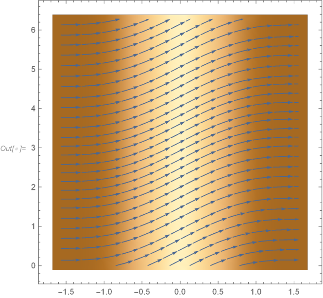
The differentials ∂Φ∂θ\frac{\partial\Phi}{\partial\theta} and ∂Φ∂ϕ\frac{\partial\Phi}{\partial\phi} give the Gramian g=(gi​j)i​j=(100cos2⁡θ)\displaystyle{g=\Big(g_{ij}\Big)_{ij}=\begin{pmatrix}1&0\\ 0&\cos^{2}\theta\end{pmatrix}} which has the associated vector field flow XS2=(1,cos2⁡θ)X_{S^{2}}=(1,\cos^{2}\theta) and stream plot as Figure 1. Observe that XS2X_{S^{2}} is divergence-free and that curl​XS2=−2​cos⁡θ​sin⁡θ.\text{curl}X_{S^{2}}=-2\cos\theta\sin\theta.

Refer to caption
Figure 1: Stream plot of the vector field XS2X_{S^{2}} on S2.S^{2}.

By the Helmholtz decomposition,

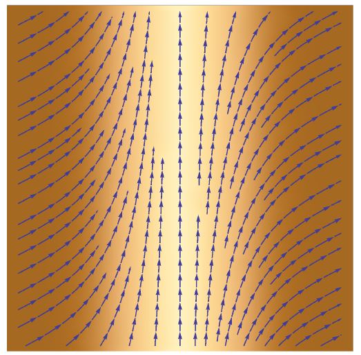
XS2=YS2+ZS2​with​YS2=XS2​and​ZS2=(−cos2⁡θ,1)​with​curl​ZS2=0.X_{S^{2}}=Y_{S^{2}}+Z_{S^{2}}~~\text{with}~~Y_{S^{2}}=X_{S^{2}}~~\text{and}~~Z_{S^{2}}=(-\cos^{2}\theta,1)~~\text{with}~~\text{curl}Z_{S^{2}}=0.

The stream plot of the Helmholtz decomposed XS2X_{S^{2}} flow is Figure 2.

Refer to caption
Figure 2: Stream plot of the decomposed XS2.X_{S^{2}}.

Finally, another main result of this work is the Stokes’ type result:

Theorem 3.10.

Let XX be smooth vector field on an open neighbourhood UU of Z⊆MZ\subseteq M with X|ZX\Big|_{Z} compactly supported and let d​AdA be the area form on Z.Z. Then the smooth function ⟨curl​(X)|Z,N^⟩\langle\text{curl}(X)\Big|_{Z},\hat{N}\rangle on Z,Z, where N^\hat{N} is the outward unit normal field along ZZ in M,M, is compactly supported and satisfies the Stokes’ type identity

∫Z⟨curl​(X)|Z,N^⟩​𝑑A=∫∂Z⟨X|∂Z,T⟩​𝑑l.\int_{Z}\langle\text{curl}(X)\Big|_{Z},\hat{N}\rangle dA=\int_{\partial Z}\langle X\Big|_{\partial Z},T\rangle dl. (3.2)
Proof.

Let η=ωX∈ΩM1​(U)\eta=\omega_{X}\in\Omega_{M}^{1}(U) be dual to X.X. Thus η|Z∈ΩZ1​(Z)\eta\Big|_{Z}\in\Omega_{Z}^{1}(Z) is compactly supported as it vanishes at points where X|ZX\Big|_{Z} vanishes. By the definition of the curl, we have ωcurl​(X)=∗(dη).\omega_{\text{curl}(X)}=\ast(d\eta). Since ∗∘∗=(−1)r⁡(n−r)\ast\circ\ast=(-1)^{r(n-r)} on rr-forms on an nn- dimensional manifold, for n=3n=3 and r=1,r=1, we have ∗∘∗=1\ast\circ\ast=1 on 11-forms on U,U, so dη=∗(ωcurl​(X)).d\eta=\ast(\omega_{\text{curl}(X)}). Similarly,

⟨curl​(X)|Z,N^⟩​d​A=(d​η)|Z\langle\text{curl}(X)\Big|_{Z},\hat{N}\rangle dA=(d\eta)\Big|_{Z}

inside of ΩZ2​(Z).\Omega_{Z}^{2}(Z). But (d​η)|Z=d⁡(η|Z)(d\eta)\Big|_{Z}=d(\eta\Big|_{Z}) since dd and pullback commute along the closed embedding of ZZ into M.M. This is compactly supported on Z.Z. For compactly supported 11-form η|Z\eta\Big|_{Z} on the 22- dimensional manifold ZZ with boundary, we get

∫Z⟨curl​(X)|Z,N^⟩​𝑑A=∫Z(𝑑η)|Z=∫Zd⁡(η|Z)=∫∂Zη|∂Z\int_{Z}\langle\text{curl}(X)\Big|_{Z},\hat{N}\rangle dA=\int_{Z}(d\eta)\Big|_{Z}=\int_{Z}d(\eta\Big|_{Z})=\int_{\partial Z}\eta\Big|_{\partial Z}

showing (3.2).

Thus our problem comes to proving the identity η|∂Z=⟨X|∂Z,T⟩​d​l∈Ω∂Z1​(∂Z).\eta\Big|_{\partial Z}=\langle X\Big|_{\partial Z},T\rangle dl\in\Omega_{\partial Z}^{1}(\partial Z). But since η|Z=ωX|Z∈ΩZ1​(Z)\eta|_{Z}=\omega_{X|_{Z}}\in\Omega_{Z}^{1}(Z) it follows that ωX|Z=ωX​Z\omega_{X|_{Z}}=\omega_{X}Z pointwise.

Let X|Z=GX|_{Z}=G and G|∂Z=H,G|_{\partial Z}=H, we want to prove that for any smooth vector field HH along ∂Z,\partial Z,

⟨H,T⟩​d​l=ωH∈Ω∂Z1​(∂Z)\langle H,T\rangle dl=\omega_{H}\in\Omega_{\partial Z}^{1}(\partial Z) (3.3)

generally for any 11-dimensional Riemannian manifold CC with length form d​ldl dual to the tangent field T.T. Evaluating both sides of (3.3) at a point p∈C,p\in C, we obtain a 11-dimensional real vector space VV endowed with an inner product. So, let V=Tp​C,V=T_{p}C, if v∈Vv\in V with length for ϕ,\phi, and for t∈Vt\in V the vector dual to ϕ\phi we have ⟨v,t⟩​ϕ=⟨v,⋅⟩\langle v,t\rangle\phi=\langle v,\cdot\rangle is in the dual space. It suffices to check this equality when evaluating both sides on the basis {t}.\{t\}. But since ϕ⁡(t)=1\phi(t)=1 by the definition of t,t, the result follows. ∎

4 Conclusion

We have constructed vorticity of vector field flows on compact smooth Riemannian manifolds through differential operators mainly the curl and the divergence operators. Many properties of vorticity on the manifolds were established and we proved that a vector field on a compact Riemannian manifold admits a unique Helmholtz decomposition. We also proved a Stokes’ type identity for the curl operator on smooth tensor fields on M.M.

This study can be extended to applications of the central ideas of the paper to physical flow problems in engineering and industry. One can as well study the vorticity of climate variabilities on the earth surface using the machinery developed in this paper. This will throw more light on the mathematical analysis of climate change.

Acknowledgement

The authors are grateful to the members of Research and Development Committee of the Department of Mathematics and Statistics of the Alex Ekwueme Federal University, Ndufu-Alike, Nigeria for their comments and suggestions that have improved the readability of this paper. We also thank members of our families for their cooperation while this research lasted. All errors are our responsibility.

References

  • [1] I. Agricla and T. Friedrich, Global Analysis - Differential Forms in Analysis, Geometry and Physics, Graduate Studies in Mathematics Volume 52, American Mathematical Society, (2002), https://bookstore.ams.org/gsm-52.
  • [2] M. F. Atiya, V. K. Patodi and I. M. Singer, Spectral asymmetry and Riemannian geometry I, Math. Proc. Cambridge Philos. Soc. 77 (1975), 43 – 69, doi:10.1017/S0305004100049410.
  • [3] C. Ba¨\ddot{a}r, Elementary Differential Geometry, Cambridge University Press, United Kingdom, (2010), doi:10.1017/CBO9780511844843.
  • [4] C. Ba¨\ddot{a}r, The curl operator on odd-dimensional manifolds, Journal of Mathematical Physics 60, (031501), (2019), doi:10.1063/1.5082528.
  • [5] M. Bauer, B. Kolev, S. Preston, Geometric investigations of a vorticity model equation, Journal of Differential Equations 260, (2016), 478 – 516, doi:10.1016/j.jde.2015.09.030.
  • [6] P. Buser, Geometry and Spectra of compact Riemann Surfaces, Birkha¨\ddot{a}user, (1992), https://link.springer.com/book/10.1007/978-0-8176-4992-0.
  • [7] O. Calin and D. C. Chang, Geometric mechanics on Riemannian manifolds: Applications to partial differential equations, Birkha¨\ddot{a}uster, Boston, Basel, Berlin, (2005), https://link.springer.com/book/10.1007/b138771.
  • [8] J. Cantarella, D. DeTurch, H. Gluck and M. Teytel, The spectrum of the curl operator on spherically symmetric domains, Physics of Plasmas 7 2766, (2000), doi:10.1063/1.874127.
  • [9] I. Chavel, Eigenvalues in Riemannian Geometry, Academic Press Inc, London, (1984), doi:10.1016/s0079-8169(08)x6051-9.
  • [10] S. Deshmukh , P. Peska and N. B. Turki, Geodesic vector fields on a Riemannian manifold, Mathematics MDPI 8, 137, (2020), doi:10.3390/math8010137.
  • [11] J. Escher, The geometry of a vorticity model equation, Communications on Pure and Applied Analysis 11, 4, (2012), 1407 – 1419, doi:10.3934/cpaa.2012.11.1407.
  • [12] T. Frankel, Homology and flows on manifolds, Annals of Mathematics 65, 2, (1957), 330 – 339, https://www.jstor.org/stable/1969965.
  • [13] A. Grigor’yam, Heat Kernels and Analysis on Manifolds, Studies in Advance Mathematics Volume 47, American Mathematical Society, (2009), doi:10.1090/amsip/047.
  • [14] B. Gustafsson, Vortex motion and geometric function theory: the role of connections, Philosophical Transactions A 377:20180341, (2019), doi:10.1098/rsta.2018.0341.
  • [15] R. Ignat and R. L. Jerrard, Interaction energy between vortices of vector fields on Riemannian surfaces, Comptes Rendus Mathematique, (2017), doi:10.1016/j.crma.2017.04.004.
  • [16] J. Jost, Riemannian Geometry and geometric analysis, 5t​h5^{th} edition, Springer-Verlag, Berlin Heidelberg, Germany, (2008), doi:10.1007/978-3-540-77341-2.
  • [17] S. C. Kim, Vortex motion on Riemannian surfaces, Journal of Korean Physical Society 59, 1, (2011), 47 – 54, doi:10.3938/jkps.59.47.
  • [18] J. M. Lee, Introduction to smooth manifolds, Graduate Texts in Mathematics, Springer, New York, (2003), https://link.springer.com/book/10.1007/978-1-4419-9982-5.
  • [19] D. Mu¨\ddot{u}ller, W. P. F. de Medeiros, R. R. de Lima, V. C. de Andrade, The divergence and curl in arbitrary basis, Revita Brasileira de Ensino de Fisica 41, 2, (2019), 1 – 7, doi:10.1590/1806-9126-RBEF-2018-0082.
  • [20] L. Omenyi and U. Uchenna, Global Analysis on Riemannian manifolds, The Australian Journal of Mathematical Analysis and Applications 16, 02, 11, (2019), 1 – 17, https://ajmaa.org/searchroot/files/pdf/v16n2/v16i2p11.pdf.
  • [21] H. C. Pak, Motion of vortex filaments in 3- manifolds, Bull. Korean Math. Soc. 42, 1, (2005), 75 – 85, doi:10.4134/BKMS.2005.42.1.075.
  • [22] L. Peng and L. Yang, The curl in seven dimensional space and its application, Approx. Theory & its Appl. 15, (1999), 66 – 80, doi:10.1007/BF02837124.
  • [23] I. Perez-Garcia, Exact solutions of the vorticity equation on the sphere as a manifold, Atmosfera 28, 3, (2015), 179 – 190, doi:10.20937/ATM.2015.28.03.03.
  • [24] B. Varayu, T S. Chew, P. Y. Lee, On the divergence theorem on manifolds, J. Math. Appl. 397, (2013), 182 – 190, doi:10.1016/j.jmaa.2012.07.042.
  • [25] H. B. da Veiga and L. C. Berselli, Navier-Stokes equation: Green matrices, vorticity direction and regularity up to the boundary, Journal of Differential Equations 246, (2009), 597 – 628, doi:10.1016/j.jde.2008.02.043.
  • [26] X. L. Xie and W. W. Mar, 2D Vorticity and stream function solutions based on curvilinear coordinates, Third International Conference on Experimental Mechanics, Proceedings of SPIE 4537, (2002), doi:10.1117/12.468772.