gulp: a prediction-based metric between representations

Enric Boix-Adserà Affiliation: MIT Email: eboix@mit.edu Hannah Lawrence Affiliation: MIT Email: hanlaw@mit.edu George Stepaniants Affiliation: MIT Email: gstepan@mit.edu Philippe Rigollet Affiliation: MIT Email: rigollet@math.mit.edu Affiliation:

Abstract

Comparing the representations learned by different neural networks has recently emerged as a key tool to understand various architectures and ultimately optimize them. In this work, we introduce gulp, a family of distance measures between representations that is explicitly motivated by downstream predictive tasks. By construction, gulp provides uniform control over the difference in prediction performance between two representations, with respect to regularized linear prediction tasks. Moreover, it satisfies several desirable structural properties, such as the triangle inequality and invariance under orthogonal transformations, and thus lends itself to data embedding and visualization. We extensively evaluate gulp relative to other methods, and demonstrate that it correctly differentiates between architecture families, converges over the course of training, and captures generalization performance on downstream linear tasks.

1 Introduction

The spectacular success of deep neural networks (DNN) witnessed over the past decade has been largely attributed to their ability to generate good representations of the data [BCV13] . But what makes a representation good? Answering this question is a necessary step towards a principled theory of DNN design. This fundamental question calls for a metric over representations as a basic primitive. Indeed, embedding representations into a metric space enables comparison, modifications and ultimately optimization of DNN architectures [LTQ+18]; see Figure 1.

In light of the practical impact of a meaningful metric over representations, this question has recently garnered significant attention, leading to a myriad of propositions such as cca, cka, and procrustes. Their relative pros and cons are currently the subject of a lively debate [DDS21, DHN+22] whose resolution calls for a theoretically grounded notion of metric.

Figure 1: t-SNE embedding of various pretrained DNN representations of the ImageNet [KSH12] dataset with gulp distance (

\lambda=10^{-2}

), colored by architecture type (gray denotes architectures that do not belong to a family). The embedding shows a good clustering of various architectures (ResNets, EfficientNets etc.), indicating that gulp captures intrinsic aspects of representations shared within an architecture family.

Our contributions.

In this work, we define a new family of metrics¹¹ 1 More specifically, we define pseudo-metrics rather than metrics. However, these can be readily turned into a metric using metric identification. This amounts to allowing equivalence classes of representations., called gulp²² 2 GULP is Uniform Linear Probing., over the space of representations. Our construction rests on a functional notion of what makes two representations similar: namely, that two representations are similar if and only if they are equally useful as inputs to downstream, linear transfer learning tasks. This idea is partially inspired by feature-based transfer learning, in which simple models adapt pretrained representations, such as Inceptionv3 [SVI+16], CLIP [RKH+21], and ELMo [PNI+18], for specific tasks [RASC14]; indeed, this is a key use for pretrained representations. Moreover, our application of linear transfer learning is reminiscent of linear probes, which were introduced by [AB17] as a tool to compare internal layers of a DNN in terms of prediction accuracy. Linear probes play a central role in the literature on hidden representations. They have been used not only to study the information captured by hidden representations [RBH20], but also to themselves define desiderata of distances between representations [DDS21]. However, previous applications of linear probing required hand-selecting the task on which prediction accuracy is measured, whereas our gulp distance provides a uniform bound over all norm-bounded tasks.

We establish various theoretical properties of the gulp pseudo-metric, including the triangle inequality (Thm 2), sample complexity (Thm 3), and vanishing cases. In particular, we show that akin to the procrustes pseudo-metric, gulp is invariant under orthogonal transformations (Thm 1) and vanishes precisely when the two representations are related by an orthogonal transformation (Thm 2).

In turn, we use gulp to produce low-dimensional embeddings of various DNNs that provide new insights on the relationship between various architectures (Figures 1, 5, and 6). Moreover, in Figure 7, we showcase a numerical experiment to demonstrate that the gulp distance between two independent networks decreases during training on the same dataset.

Related work.

This contribution is part of a growing body of work that aims at providing tools to understand and quantify the metric space of representations [RGYSD17, MRB18, KNLH19, AB17, ALM17, CLR+18, LC00, LV15, LYC+15, LLL+19, Mig19, STHH17, WHG+18, DDS21, DHN+22, CKMK22]. Several of these measures, such as svcca [RGYSD17] and pwcca [MRB18], are based on a classical canonical correlation analysis (cca) from multivariate analysis [And84]. More recently, centered kernel alignment cka [CSTEK01, CMR12, KNLH19, DHN+22] has emerged as a popular measure; see Section 2 for more details on these methods. The orthogonal procrustes metric (procrustes) is a classical tool of shape analysis [DM16] to compute the distance between labelled point clouds. Though not as conspicuous as cka-based methods in the context of DNN representations, it was recently presented under a favorable light in [DDS21].

Various desirable properties of a similarity measure between representations have been put forward. These include structural properties such as invariance or equivariance [LC00, KNLH19], as well as sanity checks such as specificity against random initialization [DDS21], for example. Such desiderata can serve as diagnostics for existing similarity measures, but fall short of providing concrete design guidelines.

Outline

The rest of the paper proceeds as follows. Section 2 lays out the derivation of gulp, as well as important theoretical properties: conditions under which it is zero, and limiting cases in terms of the regularization parameter $\lambda$ , demonstrating that it interpolates between cca and a version of cka. Section 3 establishes concentration results for the finite-sample version, justifying its use in practice. In Section 4 we validate gulp through extensive experiments³³ 3 Our code is available at https://github.com/sgstepaniants/GULP.. Finally, we conclude in Section 5.

2 The gulp distance

As stated in the introduction, the goal of this paper is to develop a pseudo-metric over the space of representations of a given dataset. Unlike previous approaches, which work with finite datasets, we take a statistical perspective and formulate the population version of our problem. We defer statistical questions arising from finite sample size to Section 3.

Let $X\in\mathbb{R}^{d}$ be a random input with distribution $P_{X}$ and let $f:\mathbb{R}^{d}\to\mathbb{R}^{k}$ denote a representation map, such as a trained DNN. The random vector $f(X)\in\mathbb{R}^{k}$ is the representation of $X$ by $f$ . We assume throughout that a representation map is centered and normalized, so that $\E[f(X)]=0$ and $\E\|f(X)\|^{2}=1$ . In particular, this normalization allows us to identify (unnormalized) representation maps $\phi,\psi$ that are related by $\psi(x)=a\phi(x)+b$ , $P_{X}$ -a.s. for $a\in\mathbb{R}$ and $b\in\mathbb{R}^{d}$ , down to a single representation of $X$ (after normalizing), which is a well-known requirement for distances between representations [KNLH19, Sec. 2.3].

We are now in a position to define the gulp distance between representations; the terminology “distance" is justified in Theorem 2. To that end, let $\phi:\mathbb{R}^{d}\to\mathbb{R}^{k}$ and $\psi:\mathbb{R}^{d}\to\mathbb{R}^{\ell}$ be two representation maps, where $\ell$ may differ from $k$ . Let $(X,Y)\in\mathbb{R}^{d}\times\mathbb{R}$ be a random pair and let $\eta(x)=\E[Y|X=x]$ denote the regression function of $Y$ onto $X$ . Moreover, for any $\lambda>0$ , let $\beta_{\lambda}$ denote the population ridge regression solution given by

\displaystyle\beta_{\lambda}=\argmin_{\beta}\E[(\beta^{\top}\phi(X)-Y)^{2}]+\lambda\|\beta\|^{2}

and similarly for $\gamma_{\lambda}$ with respect to $\psi(\cdot)$ . Since we use squared error, these only depend the distribution of $Y$ through the regression function $\eta$ .

Definition 1.

Fix $\lambda>0$ . The gulp distance between representations $\phi(X)$ and $\psi(X)$ is given by

\displaystyle d_{\lambda}(\phi,\psi):=\sup_{\eta}\Big(\E(\beta_{\lambda}^{\top}\phi(X)-\gamma_{\lambda}^{\top}\psi(X))^{2}\Big)^{\frac{1}{2}}\,,

where the supremum is taken over all regression functions $\eta$ such that $\|\eta\|_{L^{2}(P_{X})}\leq 1$ .

The gulp distance measures the discrepancy between the prediction of an optimal ridge regression estimator based on $\phi$ , and its counterpart based on $\psi$ , uniformly over all regression tasks. While this notion of distance is intuitive and motivated by a clear regression task, it is unclear how to compute it a priori. The next proposition provides an equivalent formulation of gulp, which is amenable to accurate and efficient estimation; see Section 3. It is based on the following covariance matrices:

\Sigma_{\phi}=\cov(\phi(X))=\E[\phi(X)\phi(X)^{\top}]\,\qquad\Sigma_{\psi}=\cov(\psi(X))=\E[\psi(X)\psi(X)^{\top}]

(1)

We implicitly used the centering assumption in the above definition, and the normalization condition implies that the covariance matrices have unit trace. Throughout, we assume these matrices are invertible, which is without loss of generality by projecting onto the image of the representation map. We also define the regularized inverses:

\Sigma_{\phi}^{-\lambda}:=(\Sigma_{\phi}+\lambda I_{k})^{-1}\,,\qquad\Sigma_{\psi}^{-\lambda}:=(\Sigma_{\psi}+\lambda I_{\ell})^{-1}

as well as the cross-covariance matrices $\Sigma_{\phi\psi}$ and $\Sigma_{\psi\phi}$ as follows:

\Sigma_{\phi\psi}=\E[\phi(X)\psi(X)^{\top}]=\Sigma_{\psi\phi}^{\top}\,.

(2)

Proposition 1.

Fix $\lambda\geq 0$ . The gulp distance between representations $\phi(X)$ and $\psi(X)$ satisfies

\displaystyle\boxed{\begin{aligned} d^{2}_{\lambda}(\phi,\psi)=\tr(\Sigma_{\phi}^{-\lambda}\Sigma_{\phi}\Sigma_{\phi}^{-\lambda}\Sigma_{\phi})+\tr(\Sigma_{\psi}^{-\lambda}\Sigma_{\psi}\Sigma_{\psi}^{-\lambda}\Sigma_{\psi})-2\tr(\Sigma_{\phi}^{-\lambda}\Sigma_{\phi\psi}\Sigma_{\psi}^{-\lambda}\Sigma_{\phi\psi}^{\top})\end{aligned}}

(3)

Proof.

See Appendix A.1. ∎

2.1 Structural properties

In this section, we show that gulp is invariant under orthogonal transformations and that it is a valid metric on the space of representations. We begin by establishing a third characterization of gulp that is useful for the purposes of this section; the proof can be found in Appendix A.1.

Lemma 1.

Fix $\lambda\geq 0$ . The gulp distance $d_{\lambda}(\phi,\psi)$ between the representations $\phi(X)$ and $\psi(X)$ satisfies

d_{\lambda}^{2}(\phi,\psi)=\E(\phi(X)^{\top}\Sigma_{\phi}^{-\lambda}\phi(X^{\prime})-\psi(X)^{\top}\Sigma_{\psi}^{-\lambda}\psi(X^{\prime}))^{2}\,,

where $X^{\prime}$ is an independent copy of $X$ .

We are now in a position to state our main structural results. We begin with a key invariance result.

Theorem 1.

Fix $\lambda\geq 0$ . The gulp distance $d_{\lambda}(\phi,\psi)$ between the representations $\phi(X)\in\mathbb{R}^{k}$ and $\psi(X)\in\mathbb{R}^{\ell}$ is invariant under orthogonal transformations: for any orthogonal transformations $U:\mathbb{R}^{k}\to\mathbb{R}^{k}$ and $V:\mathbb{R}^{\ell}\to\mathbb{R}^{\ell}$ , it holds

d_{\lambda}(U\circ\phi,V\circ\psi)=d_{\lambda}(\phi,\psi)

Proof.

We slightly abuse notation by identifying any orthogonal transformation $W$ to a matrix $W$ such that $W(x)=W\cdot x$ . Note that for any representation map, we have $\Sigma_{W\circ f}=W\Sigma_{f}W^{\top}$ and

\Sigma_{W\circ f}^{-\lambda}=(W\Sigma_{f}W^{\top}+\lambda WW^{\top})^{-1}=W(\Sigma_{f}^{\top}+\lambda I)W^{\top}=W\Sigma_{f}^{-\lambda}W^{\top}\,.

Hence, using Lemma 1, we get that

	$\displaystyle d_{\lambda}^{2}(U\circ\phi,V\circ\psi)$	$\displaystyle=\E(\phi(X)^{\top}U^{\top}U\Sigma_{\phi}^{-\lambda}U^{\top}U\phi(X^{\prime})-\psi(X)^{\top}V^{\top}V\Sigma_{\psi}^{-\lambda}V^{\top}V\psi(X^{\prime}))^{2}$
		$\displaystyle=\E(\phi(X)^{\top}\Sigma_{\phi}^{-\lambda}\phi(X^{\prime})-\psi(X)^{\top}\Sigma_{\psi}^{-\lambda}\psi(X^{\prime}))^{2}=d_{\lambda}^{2}(\phi,\psi)\,,$

where we used the fact that $U^{\top}U=I_{k}$ and $V^{\top}V=I_{\ell}$ . ∎

Next, we show that gulp satisfies the axioms of a metric.

Theorem 2.

Fix $\lambda>0$ . The gulp distance $d_{\lambda}(\phi,\psi)$ satisfies the axioms of a pseudometric, namely for all representation maps $\phi,\psi,\varphi$ , it holds

\displaystyle d_{\lambda}(\phi,\phi)=0,\quad\ \ d_{\lambda}(\phi,\psi)=d_{\lambda}(\psi,\phi),\quad\mbox{and}\quad d_{\lambda}(\phi,\psi)\leq d_{\lambda}(\phi,\varphi)+d_{\lambda}(\varphi,\psi)

Moreover, $d_{\lambda}(\phi,\psi)=0$ if and only if $k=\ell$ and there exists an orthogonal transformation $U$ such that $\phi(X)=U\psi(X)$ a.s.

Proof.

Lemma 1 provides an isometric embedding of representations $f\mapsto f(X)\Sigma_{f}^{-\lambda}f(X^{\prime})$ into the Hilbert space $L^{2}(P_{X}^{\otimes 2})$ . It readily yields that $d_{\lambda}$ is a pseudometric. It remains to identify for which $\phi,\psi$ it holds that $d_{\lambda}(\phi,\psi)=0$ .

The “easy” direction follows from the invariance property of Theorem 1: if $\phi$ and $\psi$ satisfy $\phi(X)=U\psi(X)$ almost surely, then $d_{\lambda}(\phi,\psi)=d_{\lambda}(U\psi,\psi)=0$ . We sketch the proof of the other direction, and defer the full proof to Appendix A.2. Define $\tilde{\phi}=(\Sigma_{\phi}+\lambda I)^{-1/2}\phi$ and $\tilde{\psi}=(\Sigma_{\psi}+\lambda I)^{-1/2}\psi$ . By Lemma 1, the condition that $d_{\lambda}(\phi,\psi)=0$ is equivalent to $\tilde{\phi}(X)^{\top}\tilde{\phi}(X^{\prime})=\tilde{\psi}(X)^{\top}\tilde{\psi}(X)$ almost surely over $X,X^{\prime}$ . So if $d_{\lambda}(\phi,\psi)=0$ , then we can leverage a classical fact that the Gram matrix of a set of vectors determines the vectors up to an isometry [HJ12], to prove that there is an orthogonal transformation $U\in\mathbb{R}^{k\times k}$ such that $\tilde{\phi}(X)=U\tilde{\psi}(X)$ almost surely over $X$ . Finally, via analyzing a homogeneous Sylvester equation, this implies that $\phi(X)=U\psi(X)$ almost surely. ∎

Note that when $\lambda=0$ , the conclusion of this theorem fails to hold: $d_{0}$ still satisfies the axioms of a pseudo-distance, but the cases for which $d_{0}(\phi,\psi)=0$ are different. This point is illustrated in the next section where we establish that $d_{0}$ is the cca distance commonly employed in the literature.

2.2 Comparison with cca, ridge-cca, cka, and procrustes

Throughout this section, we assume that $k=\ell$ for simplicity.

Ridge-cca.

Our distance is most closely related to ridge-cca, introduced by [Vin76] as a regularized version of Canonical Covariance Analysis (cca) when the covariance matrices $\Sigma_{\phi}$ or $\Sigma_{\psi}$ are close to singular. More specifically, for any $\lambda\geq 0$ , define the matrix $C_{\lambda}:=\Sigma_{\phi}^{-\lambda}\Sigma_{\phi\psi}\Sigma_{\psi}^{-\lambda}\Sigma_{\psi\phi}$ ; the ridge-cca similarity measure is defined as $\rho_{\lambda-\textsc{cca}{}}=\tr(C_{\lambda})$ . Hence, we readily see from Proposition 1 that gulp and ridge-cca are describing the same geometry over representations. To see this, recall that Lemma 1 provides an isometric embedding $f\mapsto f(X)\Sigma_{f}^{-\lambda}f(X^{\prime})$ of representation maps into $L^{2}(P_{X}^{\otimes 2})$ . While gulp is the distance on this Hilbert space, ridge-cca is the inner product.

Ridge-cca was briefly considered in the seminal work [KNLH19] but discarded because of (i) its lack of interpretability and (ii) the absence of a rule to select $\lambda$ . We argue that in fact, our prediction-driven derivation of gulp gives a clear and compelling interpretation of this geometry (as well as suggests several extensions; see Section 5). Moreover, we show that tunability of $\lambda$ is, in fact, a desirable feature that allows to represent the space of representations at various resolutions, giving various levels of information; for example, in Figure 6, higher $\lambda$ leads to a coarser clustering structure.

cca.

Due to the connection with ridge-cca, our gulp distance is related to (unregularized) cca when $\lambda=0$ . Specifically, defining $C:=\Sigma_{\phi}^{-1}\Sigma_{\phi\psi}\Sigma_{\psi}^{-1}\Sigma_{\psi\phi}$ , the mean-squared-cca similarity measure is given by (see [Eat07, Def. 10.2]):

\rho_{\textsc{cca}}(\phi,\psi):=\frac{\tr(C)}{k}=1-\frac{1}{2k}\E\big[(\phi(X)^{\top}\Sigma_{\phi}^{-1}\phi(X^{\prime})-\psi(X)^{\top}\Sigma_{\psi}^{-1}\psi(X^{\prime}))^{2}\big]\,,

where $X$ is an independent copy of $X^{\prime}$ ; the last identity can be checked directly. From Lemma 1 it can be seen that our gulp distance $d_{0}(\phi,\psi)$ with $\lambda=0$ is a linear transformation of $\rho_{\textsc{cca}}$ .

It can be checked that $\rho_{\textsc{cca}}$ takes values in $[0,1]$ , which has led researchers to simply propose $1-\rho_{\textsc{cca}}$ as a dissimilarity measure. Interestingly, this choice turns out to produce a valid (squared) metric, i.e., a dissimilarity measure that satisfies the triangle inequality. Indeed, we get that

\displaystyle d^{2}_{\textsc{cca}}(\phi,\psi)=1-\rho_{\textsc{cca}}(\phi,\psi)

\displaystyle=\frac{1}{2k}\E\big[(K(\tilde{\phi}(X),\tilde{\phi}(X^{\prime}))-K(\tilde{\psi}(X),\tilde{\psi}(X^{\prime})))^{2}\big]

where $K(u,v)=u^{\top}v$ is the linear kernel over $\mathbb{R}^{d}$ and $\tilde{\phi}:=\Sigma_{\phi}^{-1/2}\phi$ (where $\tilde{\psi}$ and $\tilde{\phi}$ are the whitened versions of $\psi$ and $\phi$ respectively). These identities have two consequences: (i) we see from Lemma 1 that $d_{\textsc{cca}{}}$ corresponds to the gulp distance with $\lambda=0$ up to a scaling factor and (ii) $d_{\textsc{cca}{}}$ is a valid pseudometric on the space of representations, since we just exhibited an isometry $T:\tilde{f}\mapsto K(\tilde{f}(X),\tilde{f}(X^{\prime}))$ with $L^{2}(P_{X}^{\otimes 2})$ . We show in Appendix A.2 that $d_{\textsc{cca}{}}(\phi,\psi)=0$ iff $\psi(X)=A\phi(X)$ a.s. for some matrix $A$ . Note that the invariance of $\rho_{\textsc{cca}{}}$ to linear transformations was previously known and criticized in [KNLH19] as arguably too strong.

cka.

In fact, thanks to the additional structure of the Hilbert space $L^{2}(P_{X}^{\otimes 2})$ , the $d_{\textsc{cca}}$ distance comes with an inner product

\langle T(\tilde{\phi}),T(\tilde{\psi})\rangle_{\textsc{cca}}:=\frac{1}{2k}\E[K(\tilde{\phi}(X),\tilde{\phi}(X^{\prime}))K(\tilde{\psi}(X),\tilde{\psi}(X^{\prime}))]\,

This observation allows us to connect cca with cka, another measure of similarity between distributions that is borrowed from classical literature on kernel methods [CSTEK01, CMR12] and that was recently made popular by [KNLH19]. Under our normalization assumptions, cka is a measure of similarity given by

	$\displaystyle\rho_{\textsc{cka}}(\phi,\psi)$	$\displaystyle=\frac{\E[K(\phi(X),\phi(X^{\prime}))K(\psi(X),\psi(X^{\prime}))]}{\sqrt{\E[K(\phi(X),\phi(X^{\prime}))^{2}]\E[K(\psi(X),\psi(X^{\prime}))^{2}]}}$
		$\displaystyle=\frac{\langle T(\phi),T(\psi)\rangle_{\textsc{cca}{}}}{\\|T(\phi)\\|_{\textsc{cca}{}}\\|T(\psi)\\|_{\textsc{cca}{}}}=\cos\left(\measuredangle(T(\phi),T(\psi))\right)\,,$

where $\|T\|_{\textsc{cca}{}}^{2}=\langle T,T\rangle_{\textsc{cca}{}}$ and $\measuredangle$ denotes the angle in the geometry induced by $\langle\cdot,\cdot\rangle_{\textsc{cca}{}}$ . In turn, $d^{2}_{\textsc{cka}{}}$ is chosen as $d^{2}_{\textsc{cka}{}}=1-\rho_{\textsc{cka}{}}$ , which does not yield a pseudometric. This observation highlights two major differences between cca and cka: the first measures inner products and works with whitened representations, while the second measures angles and works with raw representations. As illustrated in the experimental section 4 as well as in [DDS21], this additional whitening step appears to be detrimental to the overall qualities of this distance measure.

The fact that gulp with $\lambda=0$ recovers $d_{\textsc{cca}{}}$ (i.e. $d^{2}_{0}=2kd^{2}_{\textsc{cca}{}}$ ) is illustrated in Figure 2. As shown, although gulp has a roughly monotone relationship with cka, they remain quite different.

Figure 2: Empirical relationship between distances. Each point in the scatter-plot corresponds to a pair of ImageNet representations; the

x

-coordinate is the gulp distance, and the

y

-coordinate is the cca or cka distance. Although cca and gulp for

\lambda=0

are related, their relationship is not linear since the representations’ dimensionalities differ. Although cka and gulp are related for large

\lambda

, their relationship is not linear due to the difference in normalization. Appendix B.2 contains more details and comparisons, including a surprisingly strong correlation between gulp and procrustes for some values of

\lambda

procrustes.

The relationship between gulp and procrustes is not as clean as in the previous comparisons, but we include it for completeness. In the limit of infinite samples, the Procrustes distance as derived by [Sch66] is

\displaystyle d_{\text{Procrustes}}

\displaystyle=\tr(\Sigma_{\phi})+\tr(\Sigma_{\psi})-2\tr\big((\Sigma_{\phi\psi}\Sigma_{\phi\psi}^{\top})^{1/2}\big).

Our normalization implies $\tr(\Sigma_{\phi})=\tr(\Sigma_{\psi})=k$ . However, the term $\tr\big((\Sigma_{\phi\psi}\Sigma_{\phi\psi}^{\top})^{1/2}\big)$ (which is equal to the nuclear norm $||\Sigma_{\phi\psi}||_{*}$ ) is not directly comparable to the preceding distances.

3 Plug-in estimation of gulp

In practice, the distribution $P_{X}$ of $X$ is unknown, so we cannot compute the population version of gulp exactly. Instead, we have access to a sample $X_{1},\ldots,X_{n}\overset{\text{i.i.d.}}{\sim}P_{X}$ . In all of the experiments of this paper, we approximate gulp with the following plug-in estimator:

\displaystyle\boxed{\begin{aligned} \hat{d}^{2}_{\lambda,n}(\phi,\psi)&=\tr(\hat{\Sigma}_{\phi}^{-\lambda}\hat{\Sigma}_{\phi}\Sigma_{\phi}^{-\lambda}\hat{\Sigma}_{\phi})+\tr(\hat{\Sigma}_{\psi}^{-\lambda}\hat{\Sigma}_{\psi}\Sigma_{\psi}^{-\lambda}\hat{\Sigma}_{\psi})-2\tr(\hat{\Sigma}_{\phi}^{-\lambda}\hat{\Sigma}_{\phi\psi}\hat{\Sigma}_{\psi}^{-\lambda}\hat{\Sigma}_{\phi\psi}^{\top}),\end{aligned}}

where

\displaystyle\hat{\Sigma}_{\phi}=\frac{1}{n}\sum_{i=1}^{n}\phi(X_{i})\phi(X_{i})^{\top},\quad\hat{\Sigma}_{\psi}=\frac{1}{n}\sum_{i=1}^{n}\psi(X_{i})\psi(X_{i})^{\top},\quad\mbox{and}\quad\hat{\Sigma}_{\phi\psi}=\frac{1}{n}\sum_{i=1}^{n}\phi(X_{i})\psi(X_{i})^{\top}

are the empirical covariance and cross-covariance matrices, and

\displaystyle\hat{\Sigma}_{\phi}^{-\lambda}=(\hat{\Sigma}_{\phi}+\lambda I)^{-1},\quad\mbox{and}\quad\hat{\Sigma}_{\psi}^{-\lambda}=(\hat{\Sigma}_{\psi}+\lambda I)^{-1}

are the empirical inverse regularized covariance matrices. To justify our use of the plug-in estimator, we prove concentration around the population gulp distance as $n$ goes to infinity.

Theorem 3.

Assume that $\|\phi(X)\|^{2},\|\psi(X)\|^{2}\leq 1$ almost surely. Then, for any $\lambda\in(0,1)$ , $\delta>0$ , with probability at least $1-\delta$ the plug-in estimator $\hat{d}^{2}_{\lambda,n}$ satisfies

\displaystyle\left|\hat{d}_{\lambda,n}^{2}(\phi,\psi)-d_{\lambda}^{2}(\phi,\psi)\right|\lesssim\frac{1}{\lambda^{3}}\sqrt{\frac{\log((k+l)/\delta)}{n}}\,.

We defer the proof of this theorem to Appendix A.3. At a high-level, we first show that the inverse regularized covariance matrices, $(\Sigma_{\phi}+\lambda I)^{-1}$ and $(\Sigma_{\psi}+\lambda I)^{-1}$ , are well-approximated in operator norm, so the expectation of the plug-in estimator is close to the population distance. We then apply McDiarmid’s inequality to show that the plug-in estimator concentrates around its expectation. Note that the boundedness conditions on the representations are here to simplify technical arguments by appealing simply to McDiarmid’s inequality; these can be presumably be relaxed to weaker tail conditions at the cost of more involved arguments.

Figure 4 supports our theoretical result by showing convergence on pairs of networks on the ImageNet dataset. See Appendix B.3 for more details.

4 Experiments

We evaluate our distance in a variety of empirical settings, comparing to cca, cka, the classical procrustes method from shape analysis, and a variant of cca known as projection-weighted cca (pwcca); see [DDS21, Sec. 2] for definitions.

4.1 gulp captures generalization performance by linear predictors

The gulp distance is motivated by how differently linear predictors using the representations $\phi$ and $\psi$ generalize. In this section, we demonstrate that gulp indeed captures downstream generalization performance by linear predictors. We consider the representation maps $\phi_{1},\ldots,\phi_{m}$ given by $m=37$ pretrained image classification architectures on the ImageNet dataset $P_{X}$ (see Appendix B.5). For each pair of representations, we estimate the cka, cca, pwcca, and gulp distances, using the plug-in estimators on 10,000 images, sufficient to guarantee good convergence (see Figure 4).

We then draw $n=$ 5,000 images from the dataset $X_{1},\ldots,X_{n}\sim P_{X}$ , and assign a random label $Y_{k}\sim\mathcal{N}(0,1)$ to each one. For each representation $i\in[m]$ , we fit a $\lambda$ -regularized least-squares linear regression to the training data $\{(X_{k},Y_{k})\}_{k\in[n]}$ , which gives a coefficient vector $\beta_{\lambda,i}$ . Finally, for each $1\leq i<j\leq m$ , we estimate the distance $\tau_{ij}=\E_{X\sim P_{X}}[(\beta_{\lambda,i}^{\top}\phi_{i}(X)-\beta_{\lambda,j}^{\top}\phi_{j}(X))^{2}]$ between the predictions with representations $\phi_{i}$ and $\phi_{j}$ , by taking the empirical average over $3000$ samples in a test set. In Figure 4, we plot Spearman’s $\rho$ rank correlation between $\tau$ and each of the distances gulp, cka, cca, pwcca, viewed as vectors with $\binom{m}{2}$ entries, one for each pair of networks. Notice that for each $\lambda$ , the distance that attains the best correlation is the gulp distance with that $\lambda$ . This indicates that while gulp is a measure of distance that holds uniformly over prediction tasks, it retains its meaning in the context of a single prediction task.

Figure 3: Convergence of plug-in esimator as

n\to\infty

. We plot relative error

|\hat{d}^{2}_{\lambda,n}-d^{2}_{\lambda,10000}|/d^{2}_{\lambda,10000}

averaged over pairs of ImageNet DNNs.

Figure 4: gulp captures generalization of linear predictors. We plot Spearman’s

\rho

between the differences in predictions by

\lambda

-regularized linear regression, and the different distances. Results are averaged over 10 trials.

4.2 gulp distances cluster together networks with similar architectures

We are interested in how gulp can be used to compare networks of different architectures trained on the same task. We begin by comparing fully-connected ReLU networks of widths ranging from 100 to 1,000 and depths ranging from 1 to 10, trained on the MNIST handwritten digit database. Every architecture is retrained four times from different initializations (see Appendix B.1). We input all MNIST training set images into each network, save their representations at the final hidden layer, and compute cka, procrustes, and gulp distances between all pairs of representations.

Figure 5 shows Multi-Dimensional Scaling (MDS) embeddings of the distances between all MNIST networks, color coded by width and depth. For gulp with $\lambda=10^{-6}$ , the networks are largely organized according to rank of the feature matrix: networks of large width and small depth, ones whose representations have the largest rank, are the most different, as evidenced by the halo of points in the MDS plots. This outcome confirms that cca simply measures rank [KNLH19]. However, for procrustes and gulp with $\lambda=10^{-2}$ , networks become clustered by their depth, as evidenced by the striations in the MDS embeddings (plot colored by depth). Furthermore, networks of the same depth look most similar at large widths, as shown by the red centerline in the MDS embedding (plot colored by width), implying that as width increases networks converge to a shared limiting representation. Finally, gulp with $\lambda=1$ closely resembles cka and roughly organizes networks by depth. A takeaway is that gulp with $\lambda=1$ resembles procrustes and cka, and captures intrinsic characteristics such as width and depth.

Figure 5: Two dimensional MDS embedding plots of fully-connected ReLU networks colored by architecture width (top) and depth (bottom). Networks are fully-trained on MNIST and penultimate layer representations are constructed from 60,000 input train images.

Next, we show how distances between penultimate layer representations allow us to cluster pretrained networks with more complex architectures and, in turn, draw comparisons between them. To that end, we study 37 state-of-the-art models on the ImageNet Object Localization Challenge, of which the four major groups are ResNets, EfficientNets, ConvNeXts, and MobileNets (see Appendix B.1).

We compute the baseline distances between every pair of representations using 10,000 training images, and visualize them using a two-dimensional t-SNE embedding in Figure 6. Below each embedding plot we show the dendogram resulting from a hierarchical clustering of the networks based on their distances. As seen from the embeddings, when $\lambda$ increases, the gulp distance separates the ResNet architectures (blue) from the EfficientNet and ConvNeXt convolutional networks (orange and red). Compared to other distances, gulp with large $\lambda$ is able to more compactly cluster ResNets and convolutional networks separately. In Appendix B.5 we further quantify the compactness of clusterings under each distance metric by computing the standard deviation of distances within each cluster.

Figure 6: Embeddings of pwcca, cka, procrustes, and gulp distances between the last hidden layer representations of 36 pretrained ImageNet models (top) along with their hierarchical clusterings (bottom). All distance metrics separate ResNet architectures (brown dendogram leaves) from the rest of the ConvNeXt and EfficientNet architectures (pink dendogram leaves). gulp at

\lambda=1

is the most effective distance at separating ResNets from the remaining architectures.

4.3 Network representations converge in gulp distance during training

So far, we have used gulp to compare static networks taken as a blackbox representation maps. Now we use gulp to examine how representation maps evolve over the course of training. To that end, we independently train 16 Resnet18 architectures on the CIFAR10 dataset [KH+09] for 50 epochs. Figure 7 tracks the distance (averaged over all network pairs) at each epoch.

As shown, other distances change very little or even briefly increase over the course of training. For gulp with small $\lambda$ , the previous sections have demonstrated that our distance captures fine-grained differences between representations; here too, it accentuates differences in representations mid-training (visible around epoch 25). However, as $\lambda$ increases, the gulp distance differentiates less between representations, and smoothly decreases over the course of training, thus indicating that it captures intrinsic properties of the representations rather than artifacts due to random seeds.

Figure 7: Empirical distances between representations of 16 independently trained ResNet18 architectures during training, computed using 3,000 samples and averaged over all

{16\choose 2}

pairs. Distances are scaled by their average value at iteration 0.

4.4 Sensitivity versus specificity of gulp

In Appendix B.9, we reproduce the experiments of [DDS21]. Our distance compares favorably to baselines and correlates with measures of a DNN’s functional behavior. It achieves the specificity of cca and pwcca to random initializations, and improves the sensitivity of cka to out-of-distribution performance.

5 Conclusion

In this paper, we have defined a family of distances for comparing learned representations in terms of their worst-case performance gap over all $\lambda$ -regularized regression tasks. We proved convergence of the finite-sample estimator of this distance, quantified its relationship to existing notions such as cca, ridge-cca, and cka, and demonstrated promising performance in a variety of empirical settings, including the ability to distinguish between network architectures and to capture performance differences on regression tasks.

Further studying extensions beyond linear transfer learning could provide a rich direction for future work. In fact, preliminary experiments reported in Appendix B.10 indicate that, compared to section 4.1, gulp fails to predict generalization performance when the downstream task shifts from linear to logistic prediction. This suggests extending gulp to a uniform bound over other downstream predictive tasks, such as logistic regression, multi-class classification, or kernel ridge regression. Although gulp under kernel ridge regression has a closed form using the kernel trick⁴⁴ 4 This can be easily derived from vanilla ridge regression as studied in this paper (see Appendix A.4), and is related to “kernel ridge CCA” [KG03]., gulp for logistic regression does not have a closed form. This brings additional computational questions of interest that are beyond the scope of this work. Finally, it could be interesting to consider the application of gulp to knowledge distillation, or alternatively to consider adding a ridge regularization term to probing methods (inspired by gulp).

Acknowledgments and Disclosure of Funding

EB is supported by an Apple AI/ML Fellowship, and the National Science Foundation Graduate Research Fellowship under Grant No. 1745302. HL is supported by the Fannie and John Hertz Foundation and the National Science Foundation Graduate Research Fellowship under Grant No. 1745302. GS is supported by the National Science Foundation Graduate Research Fellowship under Grant No. 1745302. PR supported by NSF awards IIS-1838071, DMS- 2022448, and CCF-2106377.

References

[AB17] G. Alain and Y. Bengio. Understanding intermediate layers using linear classifier probes. In 5th International Conference on Learning Representations, ICLR 2017, Toulon, France, April 24-26, 2017, Workshop Track Proceedings, 2017.
[ALM17] S. Arora, Y. Liang, and T. Ma. A simple but tough-to-beat baseline for sentence embeddings. In International conference on learning representations, 2017.
[And84] T. W. Anderson. An introduction to multivariate statistical analysis. Wiley Series in Probability and Mathematical Statistics: Probability and Mathematical Statistics. John Wiley & Sons, Inc., New York, second edition, 1984.
[BCV13] Y. Bengio, A. C. Courville, and P. Vincent. Representation learning: A review and new perspectives. IEEE Trans. Pattern Anal. Mach. Intell., 35(8):1798–1828, 2013.
[CKMK22] T. Cui, Y. Kumar, P. Marttinen, and S. Kaski. Deconfounded representation similarity for comparison of neural networks. arXiv preprint arXiv:2202.00095, 2022.
[CLR⁺18] A. Conneau, G. Lample, M. Ranzato, L. Denoyer, and H. Jégou. Word translation without parallel data, 2018.
[CMR12] C. Cortes, M. Mohri, and A. Rostamizadeh. Algorithms for learning kernels based on centered alignment. The Journal of Machine Learning Research, 13:795–828, 2012.
[CSTEK01] N. Cristianini, J. Shawe-Taylor, A. Elisseeff, and J. Kandola. On kernel-target alignment. Advances in neural information processing systems, 14, 2001.
[DCLT18] J. Devlin, M.-W. Chang, K. Lee, and K. Toutanova. Bert: Pre-training of deep bidirectional transformers for language understanding. arXiv preprint arXiv:1810.04805, 2018.
[DDS21] F. Ding, J.-S. Denain, and J. Steinhardt. Grounding representation similarity through statistical testing. Advances in Neural Information Processing Systems, 34, 2021.
[Den12] L. Deng. The mnist database of handwritten digit images for machine learning research [best of the web]. IEEE signal processing magazine, 29(6):141–142, 2012.
[DHN⁺22] M. Davari, S. Horoi, A. Natik, G. Lajoie, G. Wolf, and E. Belilovsky. On the inadequacy of cka as a measure of similarity in deep learning. In ICLR 2022 Workshop on Geometrical and Topological Representation Learning, 2022.
[DM16] I. L. Dryden and K. V. Mardia. Statistical Shape Analysis, with Applications in R. Second Edition. John Wiley and Sons, Chichester, 2016.
[Eat07] M. L. Eaton. Multivariate statistics, volume 53 of Institute of Mathematical Statistics Lecture Notes—Monograph Series. Institute of Mathematical Statistics, Beachwood, OH, 2007.
[HJ12] R. A. Horn and C. R. Johnson. Matrix analysis. Cambridge university press, 2012.
[HZRS15] K. He, X. Zhang, S. Ren, and J. Sun. Delving deep into rectifiers: Surpassing human-level performance on imagenet classification. In Proceedings of the IEEE international conference on computer vision, pages 1026–1034, 2015.
[KB14] D. P. Kingma and J. Ba. Adam: A method for stochastic optimization. arXiv preprint arXiv:1412.6980, 2014.
[KG03] M. Kuss and T. Graepel. The geometry of kernel canonical correlation analysis. Technical Report 108, Max Planck Institute for Biological Cybernetics, January 2003.
[KH⁺09] A. Krizhevsky, G. Hinton, et al. Learning multiple layers of features from tiny images. 2009.
[KNLH19] S. Kornblith, M. Norouzi, H. Lee, and G. Hinton. Similarity of neural network representations revisited. In International Conference on Machine Learning, pages 3519–3529, 2019.
[KSH12] A. Krizhevsky, I. Sutskever, and G. E. Hinton. Imagenet classification with deep convolutional neural networks. In Advances in Neural Information Processing Systems (NeurIPS), 2012.
[LC00] A. Laakso and G. Cottrell. Content and cluster analysis: assessing representational similarity in neural systems. Philosophical psychology, 13(1):47–76, 2000.
[LIE⁺22] G. Leclerc, A. Ilyas, L. Engstrom, S. M. Park, H. Salman, and A. Madry. ffcv. https://github.com/libffcv/ffcv/, 2022.
[LLL⁺19] R. Liang, T. Li, L. Li, J. Wang, and Q. Zhang. Knowledge consistency between neural networks and beyond. In International Conference on Learning Representations, 2019.
[LTQ⁺18] R. Luo, F. Tian, T. Qin, E. Chen, and T.-Y. Liu. Neural architecture optimization. In Proceedings of the 32nd International Conference on Neural Information Processing Systems, NIPS’18, page 7827–7838, Red Hook, NY, USA, 2018. Curran Associates Inc.
[LV15] K. Lenc and A. Vedaldi. Understanding image representations by measuring their equivariance and equivalence, 2015.
[LYC⁺15] Y. Li, J. Yosinski, J. Clune, H. Lipson, and J. Hopcroft. Convergent learning: Do different neural networks learn the same representations? In Feature Extraction: Modern Questions and Challenges, pages 196–212. PMLR, 2015.
[Mig19] V. N. Miglani. Comparing learned representations of deep neural networks. Master’s thesis, Massachusetts Institute of Technology, 2019.
[MML19] R. T. McCoy, J. Min, and T. Linzen. Berts of a feather do not generalize together: Large variability in generalization across models with similar test set performance. arXiv preprint arXiv:1911.02969, 2019.
[MPL19] R. T. McCoy, E. Pavlick, and T. Linzen. Right for the wrong reasons: Diagnosing syntactic heuristics in natural language inference. arXiv preprint arXiv:1902.01007, 2019.
[MRB18] A. Morcos, M. Raghu, and S. Bengio. Insights on representational similarity in neural networks with canonical correlation. In Advances in Neural Information Processing Systems, pages 5727–5736, 2018.
[NRS⁺18] A. Naik, A. Ravichander, N. Sadeh, C. Rose, and G. Neubig. Stress test evaluation for natural language inference. arXiv preprint arXiv:1806.00692, 2018.
[PNI⁺18] M. E. Peters, M. Neumann, M. Iyyer, M. Gardner, C. Clark, K. Lee, and L. Zettlemoyer. Deep contextualized word representations. arXiv preprint arXiv:1802.05365, 2018.
[RASC14] A. S. Razavian, H. Azizpour, J. Sullivan, and S. Carlsson. Cnn features off-the-shelf: An astounding baseline for recognition. In 2014 IEEE Conference on Computer Vision and Pattern Recognition Workshops, pages 512–519, 2014.
[RBH20] A. Ravichander, Y. Belinkov, and E. Hovy. Probing the probing paradigm: Does probing accuracy entail task relevance? arXiv preprint arXiv:2005.00719, 2020.
[RGYSD17] M. Raghu, J. Gilmer, J. Yosinski, and J. Sohl-Dickstein. Svcca: Singular vector canonical correlation analysis for deep learning dynamics and interpretability. In Advances in Neural Information Processing Systems, pages 6076–6085, 2017.
[RKH⁺21] A. Radford, J. W. Kim, C. Hallacy, A. Ramesh, G. Goh, S. Agarwal, G. Sastry, A. Askell, P. Mishkin, J. Clark, et al. Learning transferable visual models from natural language supervision. In arXiv preprint arXiv:2103.00020, 2021.
[Sch66] P. H. Schönemann. A generalized solution of the orthogonal procrustes problem. Psychometrika, 31(1):1–10, 1966.
[SPW⁺13] R. Socher, A. Perelygin, J. Wu, J. Chuang, C. D. Manning, A. Y. Ng, and C. Potts. Recursive deep models for semantic compositionality over a sentiment treebank. In Proceedings of the 2013 conference on empirical methods in natural language processing, pages 1631–1642, 2013.
[STHH17] S. L. Smith, D. H. P. Turban, S. Hamblin, and N. Y. Hammerla. Offline bilingual word vectors, orthogonal transformations and the inverted softmax, 2017.
[SVI⁺16] C. Szegedy, V. Vanhoucke, S. Ioffe, J. Shlens, and Z. Wojna. Rethinking the inception architecture for computer vision. In Computer Vision and Pattern Recognition (CVPR), 2016.
[Tro12] J. A. Tropp. User-friendly tail bounds for sums of random matrices. Foundations of computational mathematics, 12(4):389–434, 2012.
[Vin76] H. Vinod. Canonical ridge and econometrics of joint production. Journal of Econometrics, 4(2):147–166, 1976.
[WHG⁺18] L. Wang, L. Hu, J. Gu, Z. Hu, Y. Wu, K. He, and J. Hopcroft. Towards understanding learning representations: To what extent do different neural networks learn the same representation. In S. Bengio, H. Wallach, H. Larochelle, K. Grauman, N. Cesa-Bianchi, and R. Garnett, editors, Advances in Neural Information Processing Systems, volume 31, pages 9584–9593. Curran Associates, Inc., 2018.
[WNB17] A. Williams, N. Nangia, and S. R. Bowman. A broad-coverage challenge corpus for sentence understanding through inference. arXiv preprint arXiv:1704.05426, 2017.
[WSM⁺18] A. Wang, A. Singh, J. Michael, F. Hill, O. Levy, and S. R. Bowman. Glue: A multi-task benchmark and analysis platform for natural language understanding. arXiv preprint arXiv:1804.07461, 2018.
[YH20] G. Yang and E. J. Hu. Feature learning in infinite-width neural networks. arXiv preprint arXiv:2011.14522, 2020.
[ZGKS21] R. Zhong, D. Ghosh, D. Klein, and J. Steinhardt. Are larger pretrained language models uniformly better? comparing performance at the instance level. arXiv preprint arXiv:2105.06020, 2021.
[ZSQ17] Z. Zhang, Y. Song, and H. Qi. Age progression/regression by conditional adversarial autoencoder. In IEEE Conference on Computer Vision and Pattern Recognition (CVPR). IEEE, 2017.

Appendix A Deferred proofs

A.1 Alternate characterizations of gulp, proofs of Proposition 1 and Lemma 1

We provide proofs of the two alternative characterizations to the gulp distance that were claimed in the main text.

Proof of Lemma 1.

Fix a distribution of $(X,Y)$ , and let $\eta(x)=\E[Y|X=x]$ be the regression function. Since we are using squared error, with $\phi$ features the best linear predictor is $\beta_{\lambda}$ that solves

\beta_{\lambda}=\Sigma_{\phi}^{-\lambda}\E[Y\phi(X)]=\Sigma_{\phi}^{-\lambda}\E[\eta(X)\phi(X)]=\Sigma_{\phi}^{-\lambda}\int\eta(x)\phi(x)\mathrm{d}P_{X}(x)

where $P_{X}$ is the marginal distribution of $X$ . Similarly

\gamma_{\lambda}=\Sigma_{\psi}^{-\lambda}\int\eta(x)\psi(x)\mathrm{d}P_{X}(x)

In particular, for a given distribution of $(X,Y)$ , the distance between the best linear predictors is

\E(\beta_{\lambda}^{\top}\phi(X)-\gamma_{\lambda}^{\top}\psi(X))^{2}.

We rewrite this in terms of $\eta$ :

	$\displaystyle\E(\beta_{\lambda}^{\top}\phi(X)-\gamma_{\lambda}^{\top}\psi(X))^{2}$	$\displaystyle=\E\left(\int\eta(x)\left[\phi(X)^{\top}\Sigma_{\phi}^{-\lambda}\phi(x)-\psi(X)^{\top}\Sigma_{\psi}^{-\lambda}\psi(x)\right]\mathrm{d}P_{X}(x)\right)^{2}$
		$\displaystyle=\E\langle\eta,\phi(X)^{\top}\Sigma_{\phi}^{-\lambda}\phi(\boldsymbol{\cdot})-\psi(X)^{\top}\Sigma_{\psi}^{-\lambda}\psi(\boldsymbol{\cdot})\rangle_{L^{2}(P_{X})}^{2}$

Therefore to sup out the distribution over $Y$ , we take the sup of $\eta$ such that $\|\eta\|_{L^{2}(P_{X})}\leq 1$ . It yields the claim of Lemma 1.

	$\displaystyle d_{\lambda}^{2}(\phi,\psi)$	$\displaystyle:=\sup_{\\|\eta\\|_{L^{2}(P_{X})}\leq 1}\E\langle\eta,\cdots\rangle_{L^{2}(P_{X})}^{2}$
		$\displaystyle=\E\\|\phi(X)^{\top}\Sigma_{\phi}^{-\lambda}\phi(\boldsymbol{\cdot})-\psi(X)^{\top}\Sigma_{\psi}^{-\lambda}\psi(\boldsymbol{\cdot})\\|_{L^{2}(P_{X})}^{2}$
		$\displaystyle=\E(\phi(X)^{\top}\Sigma_{\phi}^{-\lambda}\phi(X^{\prime})-\psi(X)^{\top}\Sigma_{\psi}^{-\lambda}\psi(X^{\prime}))^{2}$

where $X,X^{\prime}\sim P_{X}$ are independent. ∎

Using Lemma 1, we can easily prove Proposition 1.

Proof of Proposition 1.

Start with the characterization in Lemma 1, expand the square and use the cylicity and linearity of the trace:

	$\displaystyle d^{2}_{\lambda}(\phi,\psi)$	$\displaystyle=\E(\phi(X)^{\top}\Sigma_{\phi}^{-\lambda}\phi(X^{\prime})\phi(X^{\prime})^{\top}\Sigma_{\phi}^{-\lambda}\phi(X))$
		$\displaystyle\quad+\E(\psi(X)^{\top}\Sigma_{\psi}^{-\lambda}\psi(X^{\prime})\psi(X^{\prime})^{\top}\Sigma_{\psi}^{-\lambda}\psi(X))$
		$\displaystyle\quad-2\E(\phi(X)^{\top}\Sigma_{\phi}^{-\lambda}\phi(X^{\prime})\psi(X^{\prime})^{\top}\Sigma_{\psi}^{-\lambda}\psi(X))$
		$\displaystyle=\tr\E(\Sigma_{\phi}^{-\lambda}\phi(X^{\prime})\phi(X^{\prime})^{\top}\Sigma_{\phi}^{-\lambda}\phi(X)\phi(X)^{\top})$
		$\displaystyle\quad+\tr\E(\Sigma_{\psi}^{-\lambda}\psi(X^{\prime})\psi(X^{\prime})^{\top}\Sigma_{\psi}^{-\lambda}\psi(X)\psi(X)^{\top})$
		$\displaystyle\quad-2\tr\E(\Sigma_{\phi}^{-\lambda}\phi(X^{\prime})\psi(X^{\prime})^{\top}\Sigma_{\psi}^{-\lambda}\psi(X)\phi(X)^{\top})$
		$\displaystyle=\tr(\Sigma_{\phi}^{-\lambda}\Sigma_{\phi}\Sigma_{\phi}^{-\lambda}\Sigma_{\phi})+\tr(\Sigma_{\psi}^{-\lambda}\Sigma_{\psi}\Sigma_{\psi}^{-\lambda}\Sigma_{\psi})-2\tr(\Sigma_{\phi}^{-\lambda}\Sigma_{\phi\psi}\Sigma_{\psi}^{-\lambda}\Sigma_{\phi\psi}^{\top}).$

∎

A.2 gulp is a distance, proof of Theorem 2

We complete the proof of Theorem 2 by characterizing when the gulp distance is zero in the following lemma.

Lemma 2 (Characterization for when gulp is zero, for $\lambda>0$ ).

For any $\lambda>0$ , the two representation maps $\phi:\mathbb{R}^{d}\to\mathbb{R}^{k},\psi:\mathbb{R}^{d}\to\mathbb{R}^{l}$ have zero gulp distance, $d_{\lambda}(\phi,\psi)=0$ , if and only if $k=l$ andthere exists an orthogonal transformation $U\in\mathbb{R}$ such that $\phi(X)=U\psi(X)$ a.s.

Proof of Lemma 2.

In the main text it was shown that if $\phi$ and $\psi$ are related by an orthogonal transformation, then $d_{\lambda}(\phi,\psi)=0$ . It remains to prove the converse direction, which is more involved. Define $\tilde{\phi}(x)=(\Sigma_{\phi}+\lambda I)^{-1/2}\phi(x)$ and $\tilde{\psi}(x)=(\Sigma_{\psi}+\lambda I)^{-1/2}\psi(x)$ . We make the following claim, whose proof we defer:

Claim 1.

Let $\lambda>0$ and suppose $d_{\lambda}(\phi,\psi)=0$ . Then $k=l$ and there is an orthogonal transformation $U\in\mathbb{R}^{k\times k}$ such that $\tilde{\phi}(X)=U\tilde{\psi}(X)$ almost surely.

Let $U\in\mathbb{R}^{k\times k}$ be the orthogonal transformation guaranteed by the above claim. We can write

	$\displaystyle\Sigma_{\phi}$	$\displaystyle=\E[\phi(X)\phi(X)^{\top}]$
		$\displaystyle=(\Sigma_{\phi}+\lambda I)^{1/2}U(\Sigma_{\psi}+\lambda I)^{-1/2}\E[\psi(X)\psi(X)^{\top}](\Sigma_{\psi}+\lambda I)^{-1/2}U^{\top}(\Sigma_{\phi}+\lambda I)^{1/2}$
		$\displaystyle=(\Sigma_{\phi}+\lambda I)^{1/2}U(\Sigma_{\psi}+\lambda I)^{-1/2}\Sigma_{\psi}(\Sigma_{\psi}+\lambda I)^{-1/2}U^{\top}(\Sigma_{\phi}+\lambda I)^{1/2}.$

Since $\Sigma_{\phi}$ and $(\Sigma_{\phi}+\lambda I)^{1/2}$ commute, and similarly for $\Sigma_{\psi}$ and $(\Sigma_{\psi}+\lambda I)^{1/2}$ , we have

\displaystyle\Sigma_{\phi}(\Sigma_{\phi}+\lambda I)^{-1}=U\Sigma_{\psi}(\Sigma_{\psi}+\lambda I)^{-1}U^{\top}.

Write the SVDs $\Sigma_{\phi}=V_{\phi}D_{\phi}V_{\phi}^{\top}$ and $\Sigma_{\psi}=V_{\psi}D_{\psi}V_{\psi}^{\top}$ . Then

\displaystyle D_{\phi}(D_{\phi}+\lambda I)^{-1}V_{\phi}^{\top}UV_{\psi}=V_{\phi}^{\top}UV_{\psi}D_{\psi}(D_{\psi}+\lambda I)^{-1}.

(4)

Define the diagonal matrices $\Lambda_{\phi}=D_{\phi}(D_{\phi}+\lambda I)^{-1}$ and $D_{\psi}(D_{\psi}+\lambda I)^{-1}$ , and define the orthogonal matrix $M=V_{\phi}^{\top}UV_{\psi}$ . Equation (4) is a homogeneous Sylvester equation:

\displaystyle\Lambda_{\phi}M=M\Lambda_{\psi}.

Therefore $(\Lambda_{\psi})_{ii}=(\Lambda_{\phi})_{jj}$ if $M_{ij}\neq 0$ . Since $f:\mathbb{R}_{+}\to[0,1]$ defined by $f(x)=\frac{x}{x+\lambda}$ is invertible, this implies that $(D_{\phi})_{ii}=(D_{\psi})_{jj}$ if $M_{ij}\neq 0$ . From this it follows that

\displaystyle(D_{\phi}+\lambda I)^{-1/2}M(D_{\psi}+\lambda I)^{1/2}=M.

Plugging in $M$ and rearranging, we obtain

\displaystyle U^{\top}V_{\phi}^{\top}(D_{\phi}+\lambda I)^{-1/2}V_{\phi}U=V_{\psi}(D_{\psi}+\lambda I)^{-1/2}V_{\psi}^{\top},

which simplifies to

\displaystyle U^{\top}(\Sigma_{\phi}+\lambda I)^{-1/2}U=(\Sigma_{\psi}+\lambda I)^{-1/2}.

By combining this with the guarantee from Claim 1 that $\phi(X)=(\Sigma_{\phi}+\lambda I)^{1/2}U(\Sigma_{\psi}+\lambda I)^{-1/2}\psi(X)$ almost surely, we obtain

\displaystyle\phi(X)=U\psi(X),

almost surely. This shows the converse direction of the theorem. ∎

We conclude with a proof of the claim.

Proof of Claim 1.

Let $(X_{1},\ldots,X_{n},\ldots)$ be an infinite sequence of i.i.d copies of $X$ . For each $n$ , let

A_{n}=[\tilde{\phi}(X_{1}),\ldots,\tilde{\phi}(X_{n})]\in\mathbb{R}^{k\times n},\quad B_{n}=[\tilde{\psi}(X_{1}),\ldots,\tilde{\psi}(X_{n})]\in\mathbb{R}^{l\times n}.

Since $d_{\lambda}(\phi,\psi)=0$ , by the characterization of gulp in Lemma 1 we have $\tilde{\phi}(X)^{\top}\tilde{\phi}(X^{\prime})=\tilde{\psi}^{\top}(X)\tilde{\psi}(X^{\prime})$ almost surely, so $A_{n}^{\top}A_{n}=B_{n}^{\top}B_{n}$ almost surely. Suppose without loss of generality that $l\leq k$ . Then by Theorem 7.3.11 of [HJ12], we can construct a semi-orthogonal $U_{n}\in\mathbb{R}^{l\times k}$ such that $A_{n}=U_{n}B_{n}$ almost surely. Define the event

E_{1}=\{A_{n}=U_{n}B_{n}\mbox{ for all }n\geq 1\}.

Taking a union bound over countably many $n$ , we see that $E_{1}$ holds almost surely.

Define $W=\mathrm{span}\{\tilde{\psi}(X_{i})\}_{i=1}^{\infty}$ . We claim that there is a deterministic vector space $V\subseteq\mathbb{R}^{l}$ such that $W=V$ almost surely. Let $W^{\prime}$ be an independent copy of $W$ . Then $W\stackrel{{\scriptstyle d}}{{=}}W+W^{\prime}$ . For any $i\in\{0,\ldots,k\}$ ,

\mathbb{P}[\mathrm{rank}(W)\leq i]=\mathbb{P}[\mathrm{rank}(W+W^{\prime})\leq i]\leq\mathbb{P}[\mathrm{rank}(W)\leq i]-\mathbb{P}[\mathrm{rank}(W)\leq i,\mbox{ and }W^{\prime}\not\subseteq W].

We conclude that $\mathbb{P}[\mathrm{rank}(W)\leq i,\mbox{ and }W^{\prime}\not\subseteq W]=0$ for all $i$ , so $\mathbb{P}[W^{\prime}\not\subseteq W]=0$ for the two independent copies. Therefore $W$ is deterministic, and equals $V$ almost surely.

Let $N=\sup\{n+1:\mathrm{span}\{\tilde{\psi}(X_{1}),\ldots,\tilde{\psi}(X_{n})\}=\mathbb{R}^{l}\}\cup\{1\}$ . Define the event that $N$ is finite,

E_{2}=\{N<\infty\}.

Since we have shown that $\mathrm{span}\{\tilde{\psi}(X_{i})\}_{i=1}^{\infty}=V$ almost surely, it follows that $E_{2}$ holds almost surely.

We now prove that the semi-orthogonal random matrix $U_{N}\in\mathbb{R}^{k\times l}$ satisfies our conditions. Under the almost-sure events $E_{1}$ and $E_{2}$ , we can write $\tilde{\psi}(X_{N+1})=\sum_{i=1}^{N}\lambda_{i}\tilde{\psi}(X_{i})$ , and it holds that

\displaystyle\tilde{\phi}(X_{N+1})

\displaystyle=U_{N+1}\tilde{\psi}(X_{N+1})=\sum_{i=1}^{N}\lambda_{i}U_{N+1}\tilde{\psi}(X_{i})=\sum_{i=1}^{N}\lambda_{i}\tilde{\phi}(X_{i})=\sum_{i=1}^{N}\lambda_{i}U_{N}\tilde{\psi}(X_{i})=U_{N}\tilde{\psi}(X_{N+1}).

Since events $E_{1}$ and $E_{2}$ hold almost surely, and $X_{N+1}$ is independent of $N$ and $X_{1},\ldots,X_{N}$ ,

\displaystyle\mathbb{P}[\tilde{\phi}(X)=U_{N}\tilde{\psi}(X)]

\displaystyle=\mathbb{P}[\tilde{\phi}(X_{N+1})=U_{N}\tilde{\psi}(X_{N+1})]=1.

So we conclude that there is a deterministic semi-orthogonal matrix $U\in\mathbb{R}^{k\times l}$ such that $\tilde{\phi}(X)=U\tilde{\psi}(X)$ almost surely. Finally, recall that we have assumed that $\Sigma_{\phi}$ and $\Sigma_{\psi}$ are invertible. Therefore $k=\rank(\Sigma_{\phi})=\rank(\Sigma_{\tilde{\phi}})\leq\min(\rank(U),\rank(\Sigma_{\tilde{\psi}}))=\min(\rank(U),\rank(\Sigma_{\psi}))=\min(\rank(U),l)$ . We conclude that $k=l$ , and $U\in\mathbb{R}^{k\times k}$ is an orthogonal transformation. ∎

For $\lambda=0$ , we also characterize when the gulp distance is zero. Since gulp corresponds to the cca distance, with slightly different normalization, this is also a characterization of when the cca distance is zero.

Lemma 3 (Characterization for when gulp is zero, for $\lambda=0$ ).

If $\lambda=0$ , the two representation maps $\phi:\mathbb{R}^{d}\to\mathbb{R}^{k}$ and $\psi:\mathbb{R}^{d}\to\mathbb{R}^{l}$ have zero gulp distance, $d_{0}(\phi,\psi)=0$ , if and only if $k=l$ and there exists an invertible linear transformation $M\in\mathbb{R}^{k\times k}$ such that $\phi(X)=M\psi(X)$ a.s.

Proof.

For the “easy” direction, suppose that $k=l$ and $\phi=M\psi$ for an invertible $M\in\mathbb{R}^{k\times k}$ . Then $\Sigma_{\phi}=M\Sigma_{\psi}M^{\top}$ and $\Sigma_{\phi\psi}=M\Sigma_{\psi}$ . Using the characterization of gulp from Proposition 1, we obtain

	$\displaystyle d_{0}^{2}(\phi,\psi)$	$\displaystyle=\tr(\Sigma_{\phi}^{-1}\Sigma_{\phi}\Sigma_{\phi}^{-1}\Sigma_{\phi})+\tr(\Sigma_{\psi}^{-1}\Sigma_{\psi}\Sigma_{\psi}^{-1}\Sigma_{\psi})-2\tr(\Sigma_{\phi}^{-1}\Sigma_{\phi\psi}\Sigma_{\psi}^{-1}\Sigma_{\phi\psi}^{\top})$
		$\displaystyle=\tr(I_{k})+\tr(I_{k})-2\tr((M^{-1})^{\top}\Sigma_{\psi}^{-1}M^{-1}M\Sigma_{\psi}\Sigma_{\psi}^{-1}\Sigma_{\psi}(M^{-1})^{\top})$
		$\displaystyle=k+k-2\tr(I_{k})$
		$\displaystyle=0.$

For the converse direction, we construct the representations $\tilde{\phi}=\Sigma^{-1/2}_{\phi}\phi$ and $\tilde{\psi}=\Sigma^{-1/2}_{\psi}\psi$ . By the characterization of gulp in Lemma 1, the condition $d_{0}(\phi,\psi)=0$ implies that $\tilde{\phi}(X)^{\top}\tilde{\phi}(X^{\prime})=\tilde{\psi}(X)^{\top}\tilde{\psi}(X^{\prime})$ , almost surely over independent $X,X^{\prime}\sim P_{X}$ . Therefore, analogous reasoning to Claim 1 applies, and implies that $k=l$ and that there is an orthogonal transformation $U$ such that $\tilde{\phi}(X)=U\tilde{\psi}$ almost surely. So $\phi(X)=\Sigma_{\phi}^{1/2}U\Sigma_{\psi}^{-1/2}\psi(X)$ , almost surely. ∎

A.3 Convergence of plug-in estimator, proof of Theorem 3

In order to prove Theorem 3, we first show the following lemma.

Lemma 4.

There is a universal constant $C>0$ , such that for any $B$ such that $\|\phi(X)\|^{2},\|\psi(X)\|^{2}\leq B$ almost surely, and for any $\lambda>0$ , the plug-in estimator $\hat{d}^{2}_{\lambda,n}$ converges to the population distance $d_{\lambda}^{2}$ , with the following guarantee for any $t>0$ and any number of samples $n>0$ ,

\displaystyle\mathbb{P}[|\hat{d}^{2}_{\lambda,n}(\phi,\psi)-d_{\lambda}^{2}(\phi,\psi)|\geq t+4B^{2}/(n\lambda^{2})]\leq\exp(-Cnt^{2}\lambda^{4}/B^{4})+(k+l)\exp(-Cnt^{2}\lambda^{6}/B^{6}).

Proof.

By the expanding the square and using cyclicity and linearity of the trace, similarly to the proof of Proposition 1, the plug-in estimator can alternatively be written as:

\displaystyle\hat{d}^{2}_{\lambda,n}(\phi,\psi)=\frac{1}{n^{2}}\sum_{i,j=1}^{n}(\phi(X_{i})^{\top}(\hat{\Sigma}_{\phi}+\lambda I)^{-1}\phi(X_{j})-\psi(X_{i})^{\top}(\hat{\Sigma}_{\psi}+\lambda I)^{-1})\psi(X_{j}))^{2}.

(5)

For the analysis, also define the plug-in estimator, but with the true covariance matrices,

\displaystyle\tilde{d}^{2}_{\lambda,n}(\phi,\psi)=\frac{1}{n^{2}}\sum_{i,j=1}^{n}(\phi(X_{i})^{\top}(\Sigma_{\phi}+\lambda I)^{-1}\phi(X_{j})-\psi(X_{i})^{\top}(\Sigma_{\psi}+\lambda I)^{-1})\psi(X_{j}))^{2}.

(6)

We bound the error between the plug-in estimator and the true distance by the triangle inequality:

\displaystyle|\hat{d}^{2}_{\lambda,n}(\phi,\psi)-d_{\lambda}^{2}(\phi,\psi)|

\displaystyle\leq\underbrace{|\hat{d}^{2}_{\lambda,n}(\phi,\psi)-\tilde{d}^{2}_{\lambda,n}(\phi,\psi)|}_{\text{Term 1}}+\underbrace{|\tilde{d}^{2}_{\lambda,n}(\phi,\psi)-d_{\lambda}^{2}(\phi,\psi)|}_{\text{Term 2}}.

(7)

We bound Term 1 and Term 2 separately, stating our bounds in the following claims.

Claim 2 (Bound on Term 1).

Under the conditions of Lemma 4, for any $t>0$ ,

\displaystyle\mathbb{P}[|\hat{d}^{2}_{\lambda,n}(\phi,\psi)-\tilde{d}^{2}_{\lambda,n}(\phi,\psi)|\geq t]\leq(k+l)e^{-nt^{2}\lambda^{6}/(2048B^{6})}

Proof.

For any $i,j\in[n]$ , define $\hat{T}_{ij,\phi}=\phi(X_{i})^{\top}(\hat{\Sigma}_{\phi}+\lambda I)^{-1}\phi(X_{j})$ and $T_{ij,\phi}=\phi(X_{i})^{\top}\Sigma_{\phi}+\lambda I)^{-1}\phi(X_{j})$ . We have

\displaystyle|\hat{T}_{ij,\phi}-T_{ij,\phi}|

\displaystyle\leq B\|(\hat{\Sigma}_{\phi}+\lambda I)^{-1}-(\Sigma_{\phi}+\lambda I)^{-1}\|,

and

\displaystyle|\hat{T}_{ij,\phi}|,|T_{ij,\phi}|\leq B\|(\hat{\Sigma}_{\phi}+\lambda I)^{-1}\|\leq B/\lambda.

Analogous definitions and inequalities hold if we replace $\phi$ by $\psi$ . Therefore,

	$\displaystyle\|\hat{d}^{2}_{\lambda,n}(\phi,\psi)-$	$\displaystyle\tilde{d}^{2}_{\lambda,n}(\phi,\psi)\|$
		$\displaystyle=\|\frac{1}{n^{2}}\sum_{i,j=1}^{n}(\hat{T}_{ij,\phi}-\hat{T}_{ij,\psi})^{2}-(T_{ij,\phi}-T_{ij,\psi})^{2}\|$
		$\displaystyle=\|\frac{1}{n^{2}}\sum_{i,j=1}^{n}(\hat{T}_{ij,\phi}-\hat{T}_{ij,\psi}-T_{ij,\phi}+T_{ij,\psi})(\hat{T}_{ij,\phi}-\hat{T}_{ij,\psi}+T_{ij,\phi}-T_{ij,\psi})\|$
		$\displaystyle\leq 4B^{2}(\\|(\hat{\Sigma}_{\phi}+\lambda I)^{-1}-(\Sigma_{\phi}+\lambda I)^{-1}\\|+\\|(\hat{\Sigma}_{\psi}+\lambda I)^{-1}-(\Sigma_{\psi}+\lambda I)^{-1}\\|)/\lambda.$

So the bound on Term 1 follows from combining with the following technical claim:

Claim 3.

For any $t>0$ ,

\displaystyle\mathbb{P}[\|(\hat{\Sigma}_{\phi}+\lambda I)^{-1}-(\Sigma_{\phi}+\lambda I)^{-1}\|\geq t]\leq ke^{-nt^{2}\lambda^{4}/(32B^{2})}.

(8)

\displaystyle\mathbb{P}[\|(\hat{\Sigma}_{\psi}+\lambda I)^{-1}-(\Sigma_{\psi}+\lambda I)^{-1}\|\geq t]\leq le^{-nt^{2}\lambda^{4}/(32B^{2})}.

(9)

∎

Proof of Claim 3.

We prove the claim for $\phi$ , since the reasoning for $\psi$ is analogous. First, let us prove that $\hat{\Sigma}_{\phi}$ concentrates around $\Sigma_{\phi}$ in operator norm. For each $i\in[n]$ , let $Z_{i}=\frac{1}{n}\left(\phi(X_{i})\phi(X_{i})^{\top}-\Sigma_{\phi}\right)$ , which is self-adjoint, satisfies $\E[Z_{i}]=0$ and has operator norm bounded by $\|Z_{i}^{2}\|\leq\frac{1}{n^{2}}\left(2\|\phi(X_{i})\phi(X_{i})^{\top}\|^{2}+2\|\Sigma_{\phi}\|^{2}\right)\leq 4B^{2}/n^{2}$ almost surely. So applying the matrix Hoeffding inequality (Theorem 1.3 of [Tro12]) to $\hat{\Sigma}_{\phi}=\sum_{i=1}^{n}Z_{i}$ , we have, for any $t>0$ ,

\displaystyle\mathbb{P}[\|\hat{\Sigma}_{\phi}-\Sigma_{\phi}\|\geq t]\leq ke^{-t^{2}n/(32B^{2})}.

Now let us show that $(\hat{\Sigma}_{\phi}+\lambda I)^{-1}$ concentrates to $(\Sigma_{\phi}+\lambda I)^{-1}$ in operator norm. Since $0\lesssim\hat{\Sigma}_{\phi},\Sigma_{\phi}$ , for any $v\in\mathbb{R}^{k}$ , we have

	$\displaystyle\\|((\hat{\Sigma}_{\phi}+\lambda I)^{-1}-(\Sigma_{\phi}+\lambda I)^{-1})v\\|$	$\displaystyle\leq\frac{1}{\lambda}\\|(I-(\hat{\Sigma}_{\phi}+\lambda I)(\Sigma_{\phi}+\lambda I)^{-1})v\\|$
		$\displaystyle=\frac{1}{\lambda}\\|((\hat{\Sigma}_{\phi}-\Sigma_{\phi})(\Sigma_{\phi}+\lambda I)^{-1})v\\|$
		$\displaystyle\leq\frac{1}{\lambda^{2}}\\|\hat{\Sigma}_{\phi}-\Sigma_{\phi}\\|\\|v\\|.$

∎

We now bound the second term in (7).

Claim 4 (Bound on Term 2).

Under the conditions of Lemma 4, for any $t>0$ ,

\displaystyle\mathbb{P}[|\tilde{d}^{2}_{\lambda,n}(\phi,\psi)-d_{\lambda}^{2}(\phi,\psi)|\geq 4B^{2}/(n\lambda^{2})+t]\leq\exp(-t^{2}\lambda^{4}n/(8B^{4})).

Proof.

Write $\tilde{d}^{2}_{\lambda,n}(\phi,\psi)=\sum_{i,j=1}^{n}s_{ij}$ , where

s_{ij}=\frac{1}{n^{2}}(\phi(X_{i})^{\top}(\Sigma_{\phi}+\lambda I)^{-1}\phi(X_{j})-\psi(X_{i})^{\top}(\Sigma_{\psi}+\lambda I)^{-1})\psi(X_{j}))^{2}

is the $i,j$ term in the sum. Since $\|(\hat{\Sigma}_{\phi}+\lambda I)^{-1}\|,\|(\hat{\Sigma}_{\psi}+\lambda I)^{-1}\|\leq 1/\lambda$ , and $\|\phi(X_{i})\|^{2},\|\psi(X_{i})\|^{2}\leq B$ , we have almost surely

|s_{ij}|\leq\frac{4B^{2}}{n^{2}\lambda^{2}}.

Furthermore, term $s_{ij}$ only depends on $X_{i}$ and $X_{j}$ . Therefore, by McDiarmid’s inequality,

\displaystyle\mathbb{P}[|\tilde{d}^{2}_{\lambda,n}(\phi,\psi)-\E[\tilde{d}^{2}_{\lambda,n}(\phi,\psi)]|\geq t]\leq\exp(-t^{2}\lambda^{4}n/(8B^{4})),

(10)

where we have used that $|\sum_{j=1}^{n}s_{ij}|\leq 4B^{2}/(n\lambda^{2})$ for each $i$ . Finally, we bound the difference between $\tilde{d}^{2}_{\lambda,n}$ and $d_{\lambda}^{2}$ in expectation over the samples. Notice that if $i\neq j$ we have $\E[s_{ij}]=d_{\lambda}^{2}(\phi,\psi)/n^{2}$ . So the only terms that can add bias are the diagonal terms $s_{ii}$ , so

\displaystyle|d_{\lambda}^{2}(\phi,\psi)-\E[\tilde{d}^{2}_{\lambda,n}(\phi,\psi)]|\leq\sum_{i=1}^{n}|s_{ii}|\leq 4B^{2}/(n\lambda^{2})

(11)

Combining (10) and (11) proves the claim. ∎

Combining Claims 2 and 4 with the triangle inequality (7) proves Lemma 4.

∎

Theorem 3 is now a simple consequence of Lemma 4.

Proof of Theorem 3.

Under the conditions of Theorem 3, we have $\|\phi(X)\|^{2},\|\psi(X)\|^{2}\leq 1$ almost surely and $\lambda\in(0,1)$ . For any $t>0$ , Lemma 4 implies

\displaystyle\mathbb{P}[|\hat{d}^{2}_{\lambda,n}(\phi,\psi)-d_{\lambda}^{2}(\phi,\psi)|\geq t+4/(n\lambda^{2})]\leq\exp(-Cnt^{2}\lambda^{4})+(k+l)\exp(-Cnt^{2}\lambda^{6}).

Let $0<\delta\leq 1$ and let $t=\frac{2}{C\lambda^{3}}\sqrt{\frac{\log((k+l)/\delta)}{n}}$ . Then

\mathbb{P}[|\hat{d}_{\lambda,n}^{2}(\phi,\psi)-d_{\lambda}^{2}(\phi,\psi)|\geq t+4/(n\lambda^{2})]<\delta/2+\delta/2=\delta\,.

Finally, since $\lambda\in(0,1)$ we have

\frac{1}{\lambda^{3}}\sqrt{\frac{\log((k+l)/\delta)}{n}}\gtrsim t+4/(n\lambda^{2}),

which proves the theorem. ∎

A.4 Transfer learning distance under kernel ridge regression

Consider comparing the predictors output by kernel ridge regression with some kernel $K(x,y)=\langle\tau(x),\tau(y)\rangle$ , applied to different representations. This corresponds to the case $\mathcal{F}=\{f_{\beta}(\cdot):\>f_{\beta}(x)=\beta^{\top}\tau(x)\}$ and $r(f_{\beta})=||\beta||_{2}^{2}$ . Although $\tau$ may be high or even infinite dimensional, we now show that computing gulp under this $\mathcal{F}$ requires only access to $K(\cdot,\cdot)$ , and not $\tau$ directly.

This is equivalent to defining new representations $\phi^{\prime}=\tau\circ\phi$ and $\psi^{\prime}=\tau\circ\phi$ , and computing $d_{\phi}(\phi^{\prime},\psi^{\prime})$ . However, $\tau$ may be high or even infinite-dimensional; traditionally in kernel ridge regression, one only wishes to compute $K(\cdot,\cdot)$ but never $\tau$ explicitly. Here, we show that $d_{\lambda}(\phi,\psi)$ is computable in terms of only inner products $\langle\phi(x),\phi(y)\rangle$ and $\langle\psi(x),\psi(y)\rangle$ , or put differently, that $d_{\lambda}(\phi,\psi)$ can be written in terms of only the kernel functions associated with $\phi$ and $\psi$ . By applying this result to $\phi^{\prime}$ and $\psi^{\prime}$ , this implies we only need to access $\langle\phi^{\prime}(x),\phi^{\prime}(y)\rangle=\langle\tau(\phi(x)),\tau(\phi(y))\rangle=K(\phi(x),\phi(y))$ .

Recall that $d_{\lambda}(\phi,\psi)^{2}=\tr((\Sigma_{\phi}+\lambda I)^{-1}\Sigma_{\phi}(\Sigma_{\phi}+\lambda I)^{-1}\Sigma_{\phi})+\tr((\Sigma_{\psi}+\lambda I)^{-1}\Sigma_{\psi}(\Sigma_{\psi}+\lambda I)^{-1}\Sigma_{\psi})-2\tr((\Sigma_{\phi}+\lambda I)^{-1}\Sigma_{\phi\psi}(\Sigma_{\psi}+\lambda I)^{-1}\Sigma_{\phi\psi}^{\top})$ . We prove the result for the finite sample case discussed in 3, where we approximate $\Sigma_{\phi}=VV^{\top}$ , $\Sigma_{\psi}=WW^{\top}$ . Here, $V$ consists of all the samples $\phi(x)$ , with number of columns equal to the number of samples. By the kernel trick, $(\Sigma_{\phi}+\lambda I)^{-1}\Sigma_{\phi}=(VV^{\top}+\lambda I)^{-1}VV^{\top}=V(V^{\top}V+\lambda I)^{-1}V^{\top}$ . Thus:

	$\displaystyle\tr((\Sigma_{\phi}+\lambda I)^{-1}\Sigma_{\phi}(\Sigma_{\phi}+\lambda I)^{-1}\Sigma_{\phi})$	$\displaystyle=\tr(V(V^{\top}V+\lambda I)^{-1}V^{\top}V(V^{\top}V+\lambda I)^{-1}V^{\top})$
		$\displaystyle=\tr((V^{\top}V+\lambda I)^{-1}V^{\top}V(V^{\top}V+\lambda I)^{-1}V^{\top}V)$

This term is expressible in terms of only $(V^{\top}V)_{ij}$ , which only depends on $\langle\phi(x_{i}),\phi(x_{j})\rangle$ for samples $x_{i}$ and $x_{j}$ . Similar reasoning holds for the term $\tr((\Sigma_{\psi}+\lambda I)^{-1}\Sigma_{\psi}(\Sigma_{\psi}+\lambda I)^{-1}\Sigma_{\psi})$ . Finally, consider the cross-term:

	$\displaystyle\tr((\Sigma_{\phi}+\lambda I)^{-1}\Sigma_{\phi\psi}(\Sigma_{\psi}+\lambda I)^{-1}\Sigma_{\phi\psi}^{\top})$	$\displaystyle=\tr((VV^{\top}+\lambda I)^{-1}VW^{\top}(WW^{\top}+\lambda I)^{-1}WV^{\top})$
		$\displaystyle=\tr(V(V^{\top}V+\lambda I)^{-1}W^{\top}W(W^{\top}W+\lambda I)^{-1})$
		$\displaystyle=\tr((V^{\top}V+\lambda I)^{-1}V^{\top}V(W^{\top}W+\lambda I)^{-1}W^{\top}W)$

Again, this term is expressible only in terms of $V^{\top}V$ and $W^{\top}W$ .

Appendix B Supplementary experiments

B.1 Experimental Setup

Here we briefly describe all of the network architectures used in this paper as well as the procedure for training them. All experiments were run on Nvidia Volta V100 GPUs.

Networks on MNIST

For the MNIST handwritten digit database [Den12], we initialize 400 fully-connected networks with ReLU activations. Each networks accepts a flattened $28\times 28$ image (784 grayscale pixels) as input and outputs at its last layer a vector of 10 probabilities for a given digit 1-10. The number of hidden layers in the networks range from 1 to 10 and the widths of all hidden layers are constant and range from 100 to 1000 in multiples of 100. Each model architecture with a fixed width and depth is randomly initialized 4 separate times with uniform Kaiming initialization [HZRS15] and zero bias. Every network is trained for 50 epochs and a batch size of 100 on all 60,000 images of the MNIST train set using the Adam optimizer [KB14] with a learning rate of $10^{-4}$ .

Networks on ImageNet

For the ImageNet Object Localization Challenge [KSH12], we use 37 state-of-the-art models downloaded both in untrained and pretrained form from the PyTorch database of models⁵⁵ 5 https://pytorch.org/vision/stable/models.html#classification. All models can be separated into the following classes

•

ResNets: regnet_x_16gf, regnet_x_1_6gf, regnet_x_32gf, regnetx_3_2_gf, regnet_x_400mf, regnet_x_800mf, regnet_x_8gf, regnet_y_16gf, regnet_y_1_6gf, regnet_y_32gf, regnet_y_3_2gf, regnet_y_400mf, regnet_y_800mf, regnet_y_8gf, resnet18, resnext50_32x4d, wide_resnet50_2
•

EfficientNets: efficientnet_b0, efficientnet_b1, efficientnet_b2, efficientnet_b3, efficientnet_b4, efficientnet_b5, efficientnet_b6, efficientnet_b7
•

MobileNets: mobilenet_v2, mobilenet_v3_small, mobilenet_v3_large
•

ConvNeXts: convnext_base, convnext_tiny, convnext_small, convnext_large
•

Miscellaneous: alexnet, googlenet, inception, mnasnet, vgg16

All models accept 3-channel RGB images of size $224\times 224$ (i.e. total dimension $3\times 224\times 224$ ). We normalize the 1,281,119 images in the train set of ImageNet to have mean $(0.485,0.456,0.406)$ and standard deviation $(0.229,0.224,0.225)$ in each RGB channel. Every models embeds the images into a latent space with dimension ranging from 400 to 4096 depending on the architecture.

Networks on CIFAR

For CIFAR [KH+09], we train 16 ResNet18 architectures from independent, random initializations for 50 epochs each using the FFCV library [LIE+22]. They were trained with batch size 512, learning rate $0.5$ on a cyclic schedule, momentum parameter $0.9$ , and with weight decay parameter $5e-4$ .

B.2 Relationship of gulp to other distances

Embeddings of ImageNet

Figure 2 of the main text compares the cka, cca, and gulp distances between pairs of representations of 37 ImageNet representations, estimated from 10,000 samples. In Figure 8, we extend the comparison to pwcca and procrustes. We note that at certain $\lambda$ , our distance has near-linear relationships with procrustes and cka.

Figure 8: Scatter plots showing relationships between network distances on ImageNet. Each point is a pair of ImageNet representations, and the

x

and

y

coordinates correspond to two distances that are being compared. There is a surprising near-linear relationship between procrustes and gulp for intermediate

\lambda

. The title of each plot shows the Pearson correlation coefficient.

Embeddings of MNIST

In Figure 9, we repeat the same experiment for MNIST embeddings with trained fully-connected networks of depths in the range from 1 to 10, and widths in $\{200,400,600,800,1000\}$ .

Figure 9: Scatter plots showing relationships between network distances of fully-connected network representations on MNIST. For

\lambda=0

, there is no straight-line relationship with CCA, since the dimensions of the representations differ, and the normalization of CCA is different from that of gulp because it depends the representation dimension. Each point is a pair of MNIST representations, and the

x

and

y

coordinates correspond to two distances that are being compared. The near-linear relationship between CKA and GULP is quite evident for large

\lambda

, as it turns out that all of the kernels are closer to having the same normalization than in the case of the ImageNet dataset. Furthermore, there is a surprising near-linear relationship between CKA and procrustes for intermediate

\lambda

. The title of each plot shows the Pearson correlation coefficient.

B.3 Convergence of the plug-in estimator

In Figure 4, we estimated the distances between $\binom{15}{2}=105$ pairs of ImageNet networks with the plug-in estimator as we increased the number of samples $n$ . We plotted the average relative error to the 10000-sample estimate. We supplement this result with Figure 10, which shows that for $n\geq 2000$ , two independent estimates of gulp have average relative error smaller than 2%. Therefore, if there is error in the plug-in estimator it is mainly due to bias, apart from roughly 2% relative error. Since the convergence in 4 indicates that the plug-in estimator is unbiased, this reinforces our claim that the plug-in estimator concentrates quickly around the true distance.

Figure 10: Relative error

|\hat{d}_{\lambda,n}^{(1)}-\hat{d}_{\lambda,n}^{(2)}|/(\hat{d}_{\lambda,n}^{(1)}+\hat{d}_{\lambda,n}^{(2)})

between plug-in estimator on two trials

\hat{d}^{(1)}_{\lambda,n}

and

\hat{d}^{(2)}_{\lambda,n}

with independent samples. We have averaged across the 66 pairs of ImageNet networks. For

\lambda=0

, due to numerical precision issues we do not plot the relative error in the estimate for

n\leq 2000

Runtime

The 12 ImageNet networks for these plots were alexnet_pretrained_rep, convnext_small_pretrained_rep, efficientnet_b0_pretrained_rep, efficientnet_b3_pretrained_rep, efficientnet_b6_pretrained_rep, inception_pretrained_rep, mobilenet_v3_large_pretrained_rep, regnet_x_1_6gf_pretrained_rep, regnet_x_400mf_pretrained_rep, regnet_y_16gf_pretrained_rep, regnet_y_3_2gf_pretrained_rep, regnet_y_8gf_pretrained_rep, subsampled from the 37 models at our disposal so as to reduce the computational burden. Generating these plots took 11 minutes with an Nvidia Volta V100 GPU. The computational cost is due to the fact that distances are computed for a range of increasing number of samples $n$ , on 66 pairs of networks and two independent trials.

B.4 gulp captures generalization performance by linear predictors

Here we supplement the experiments of Section 4.1, which show how the gulp distance captures generalization performance by linear predictors. We provide an experiment on the UTKFace dataset [ZSQ17] using the age of a face as the regression label, instead of using a random label. We consider the representation maps $\phi_{1},\ldots,\phi_{m}$ given by $m=37$ pretrained Imagenet image classification architectures, applied to the UTKFace dataset $P_{X}$ . For each pair of representations, we compute the cka, cca, pwcca, and gulp distances with the plug-in estimator on 10,000 images. We then draw $n=5000$ data points $(X_{i},Y_{i})\sim P_{X}$ , where $X_{i}$ is the face image and $Y_{i}$ is the corresponding age. The remaining experiment details are the same as in Section 4.1. For each representation $i\in[m]$ we fit a $\lambda$ -regularized least-squares linear regression to the training data $\{(X_{k},Y_{k})\}_{k\in[n]}$ , yielding a coefficient vector $\beta_{\lambda,i}$ . Finally, for each $1\leq i\leq j\leq m$ , we compute the distance $\tau_{ij}$ between predictions as an empirical average over 3000 samples in a testset. In Figure 11, we plot the Spearman $\rho$ correlations between the prediction distances $\tau_{ij}$ and the different distances between representations (similarly to Figure 4). We run one trial, since the labels are no longer random. The gulp distance again performs favorably compared to other methods. For linear regression with $\lambda=1$ and $\lambda=10^{-6}$ , the gulp distance with $\lambda=1$ and $\lambda=10^{-6}$ , respectively vastly outperform previously-proposed distances in terms of predicting generalization. For linear regression with $\lambda=10^{-4}$ and $\lambda=10^{-2}$ , gulp with $\lambda=10^{-2}$ predicts the generalization performance on par with the cka and procrustes distances. Notice that unlike the experiment with random labels, the best $\lambda$ for gulp does not exactly match the $\lambda$ used in the linear regression task, but instead is close to it.

Figure 11: gulp captures generalization of linear predictors. We plot Spearman’s

\rho

between the differences in predictions by

\lambda

-regularized linear regression, and the different distances.

B.5 gulp distances cluster together networks with similar architectures

Here we elaborate further on the experiments described in Section 4.2 on embeddings of MNIST networks. As described previously, we generate four independent copies of fully-connected ReLU networks with depths ranging from 1-10 and widths ranging from 100-1000. Network depth refers to the number of hidden layers in a model and network width refers to the width of each hidden layer. All networks are fully-trained on MNIST, and their last hidden layer representations are computed on 60,000 input images from the train set. For every pair of widths and depths $(w_{1},d_{1})$ and $(w_{2},d_{2})$ , there are four trained networks with dimensions $(w_{1},d_{1})$ and four trained networks with dimensions $(w_{2},d_{2})$ . For a given metric, we compute $4\cdot(3-1)=12$ distances between the penultimate layer representations of these networks and average them. This gives us the average distance between the penultimate layer representations of a network with dimensions $(w_{1},d_{1})$ and a network with dimensions $(w_{2},d_{2})$ . In Figure 12 (left) we show the average pwcca, cka, procrustes, and gulp distances between each pair of width-depth architectures for varying $\lambda$ . We also display the MDS embeddings of all $4\times 10\times 10$ networks colored by width and depth (center and right).

In Figure 13 we perform a very similar experiment to the one above with networks trained on CIFAR10 instead of MNIST. We generate five independent copies of fully-connected ReLU networks with depths ranging from 1-5 and widths ranging from 200-1,000. All networks are fully-trained on 60,000 images of the CIFAR10 train set by SGD in the maximal-update parametrization [YH20], where for a width-one network our hyperparameters would be learning rate $\eta=0.1$ and we would initialize weights and biases as Gaussian with standard deviation 1. The distances between their penultimate layer representations are computed using 10,000 randomly selected CIFAR10 images. Figure 13 shows the average pwcca, cka, procrustes, and gulp distances between each pair of width-depth architectures and show the MDS embeddings of all $5\times 5\times 5$ networks colored by width and depth (center and right).

Now we describe in more detail how various distance metrics cluster state-of-the-art network architectures on the ImageNet Object Localization Challenge. In Figure 14 (left) we compute the cca, pwcca, cka, procrustes, and gulp distances for five groups of networks: 17 ResNets, 8 EfficientNets, 4 ConvNeXts, and 3 MobileNets. These 32 networks are fully-trained on ImageNet and are given the same 10,000 input training images to form their last hidden layer representations. As discussed in Section 4.2, all distance metrics separate ResNet architectures (blue) from the EfficientNet and ConvNeXt convolutional networks (orange and red) with gulp at $\lambda=1$ achieving the best separation between these two clusters. To further quantify the compactness of the clusterings given by these distance metrics, we compute a standard deviation ratio for each of the five network classes. Given a distance metric, this ratio is computed as the sum of squared distances between all 36 networks divided by the sum of squared distances between networks in each class:

\text{standard deviation ratio for class }k=\Big(\frac{1}{n(n-1)}\sum_{1\leq i\neq j\leq n}d_{ij}^{2}\Big/\frac{1}{|\mathcal{C}_{k}|(|\mathcal{C}_{k}|-1)}\sum_{i\neq j\in\mathcal{C}_{k}}d_{ij}^{2}\Big)^{\frac{1}{2}}

(12)

where $n=36$ and $C_{k}\subset\{1,\dots,n\}$ is the subset of networks in class $k=1,\dots,5$ . Note that a ratio of 1 implies that the size of the cluster is equal to the average distance between any two ImageNet networks. In Figure 14 (right) we plot the standard deviation ratio for each of the five network classes. As expected, the ratios under the gulp distance increase for large $\lambda$ and the residual and convolutional network architectures become well separated at $\lambda=1$ . The cca, pwcca, cka, and procrustes distances do not achieve the same level of separation between different network architectures but are similar to the gulp distance at $\lambda=10^{-2}$ .

Now we study distances between the same ImageNet models when they are untrained and are at random initialization. Again there are 32 untrained networks consisting of 17 ResNets, 8 EfficientNets, 4 ConvNeXts, and 3 MobileNets. Each of the untrained networks is randomly initialized ten separate times and is given the same 10,000 input training images from ImageNet. We compute the cka, procrustes, and gulp distances between their penultimate layer representations which are displayed in Figure 15 (left). The distances between these networks are visualized using a two-dimensional t-SNE embedding and the standard deviation ratio (12) of each of the four groups is calculated [Figure 15 (center and right)]. Under all distance metrics we see that the ResNets (blue), EfficientNets (orange), and ConvNeXts (red) all form their own clusters. As evidenced by the standard deviation ratios, the ConvNeXt networks under the gulp distance form a tighter cluster as $\lambda$ increases. Both cka and gulp with $\lambda=1$ achieve the most compact clusterings of ResNets, EfficientNets, and ConvNeXts.

In Figure 16 for several distance metrics we display the standard deviation ratios for the five network groups before and after training. On untrained and pretrained networks, cka and procrustes are competitive with gulp at clustering ResNet, EfficientNet, and ConvNeXt architectures. However on ConvNeXt models, for untrained networks gulp achieves the highest standard deviation ratio with large $\lambda$ and for pretrained networks it achieves the highest standard deviation ratio at intermediate values of $\lambda$ .

Refer to caption — Figure 12: Average cka, procrustes, and gulp distance between last hidden layer representations of two fully-connected ReLU networks with a given width and depth (left). Networks are fully-trained on MNIST and penultimate layer representations are constructed from 60,000 input train images. Ordering of networks along rows and columns of distance matrices has outer indices as network depths 1-10 and inner indices as network widths 100-1000. Two dimensional MDS embedding plots (center and right) of all networks colored by architecture width and depth.

Figure 16: Standard deviation ratio of distances for five groups of architectures (ResNet, EfficientNet, MobileNet, and ConvNeXt) both for untrained and pretrained networks.

B.6 gulp does not strongly depend on input data distribution

Here we test how the gulp distance between network architectures depends on the distribution of the input data $X$ from which the last hidden layer representations are computed. In Figure 1 we showed a t-SNE embedding of the gulp distance ( $\lambda=10^{-2}$ ) between the last hidden layer representations of 37 networks pretrained on ImageNet. These penultimate layer representations were computed by passing 10,000 images from the ImageNet train set into each network. In Figure 17 we repeat this experiment and generate a t-SNE embedding of the gulp distance ( $\lambda=10^{-2}$ ) between ImageNet networks where each network is passed in 10,000 images from the MNIST train set. In order to input MNIST grayscale images into these networks, we convert them to RGB images where each channel has a copy of the same image and is centered and normalized as described in Section B.1. Even though all 37 networks were trained on the ImageNet train set, gulp is able to separately cluster EfficientNet, ResNet, and ConvNeXt architectures from their last hidden layer representations of MNIST images. In Figure 18 we show yet another example of this phenomenon, where gulp properly clusters ImageNet architectures when their last hidden layer representations are constructed from 10,000 face input images taken from the UTKFace train dataset [ZSQ17]. This shows that in practice the gulp distance consistently captures the same relationships between network architectures and does not strongly depend on the input data distribution used to build the network representations.

Figure 17: t-SNE embedding of penultimate layer representations of pretrained ImageNet networks with gulp distance (

\lambda=10^{-2}

), colored by architecture type (gray denotes architectures that do not belong to a family). For each network pretrained on ImageNet we input MNIST images and compute their last hidden layer representations. Even though these ImageNet networks were not trained on MNIST data, the gulp distance is able to cluster their penultimate layer representations and consistently forms groups of MobileNet, EfficientNet, ResNet, and ConvNeXt architectures. This indicates that the gulp metric does not depend strongly on the data distribution which networks are trained on.

Figure 18: t-SNE embedding of penultimate layer representations of pretrained ImageNet networks with gulp distance (

\lambda=10^{-2}

), colored by architecture type (gray denotes architectures that do not belong to a family). Contrary to Figure 1, here for each network pretrained on ImageNet we input 10,000 face images from the UTKFace train dataset and compute their last hidden layer representations. Even though these ImageNet networks were not trained on UTKFace data, the gulp distance is able to cluster their last hidden layer representations and consistently forms groups of MobileNet, EfficientNet, ResNet, and ConvNeXt architectures. This in conjunction with Figure 17 shows that the gulp metric is not overly sensitive to the input data distribution from which network representations are constructed.

B.7 Network representations converge in gulp distance during training

Here, we repeat Figure 7, but plot each distance separately and with a greater variety of regularization values $\lambda$ (see Figure 19).

Figure 19: The empirical distances between penultimate layer representations of 16 independently trained ResNet18 architectures during training, computed using

3,000

samples and averaged over all pairs. Distances are scaled by their average value at iteration

0

for the sake of comparison between metrics.

B.8 gulp distance at intermediate network layers

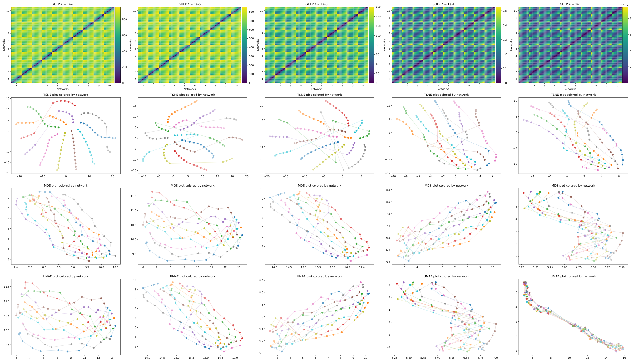
Throughout this paper, we have primarily used gulp to compare neural networks using their last hidden layer representations. Here we study how the gulp distance compares intermediate hidden layers of neural networks. Namely, we take 10 NLP BERT base models from Zhong et al. [ZGKS21] which are pretrained with different random initializations on sentences from the Multigenre Natural Language Inference (MNLI) dataset [WNB17]. Each model has 12 hidden layers and we save the representations at every hidden layer on 3,857 MNLI input train samples. In Figure 20 we plot the distance matrices for gulp at varying values of $\lambda$ between every pair of hidden layers across 10 BERT networks. We also plot the tSNE, MDS, and UMAP embeddings with each colored line representing one of the 10 BERT models. In each embedding plot, earlier layers are drawn as points with a dark hue while layers closer to the end of the network are represented by points with a faded color. As expected, for each of the BERT model the gulp distances arrange their hidden layers linearly in order from their input layer to their output layer. When $\lambda$ is small, the earlier layers of all 10 networks are grouped together while the later layers have large gulp distances between all 10 models. As $\lambda$ increases, the later layers of all 10 models also become grouped together and gulp arranges all BERT models linearly in the order of their hidden layers. Therefore, tuning the $\lambda$ parameter in gulp allows us to make distinctions between earlier and later layers of a network architecture.

B.9 Specificity versus sensitivity of gulp

Here we run three benchmark experiments of [DDS21] to compare the sensitivity and specificity of our gulp distance to cca, pwcca, cka, and procrustes.

In the first experiment, we take 10 BERT base models from Zhong et al. [ZGKS21] which are pretrained with different random initializations on sentences from the Multigenre Natural Language Inference (MNLI) dataset [WNB17]. All BERT base models have 12 hidden layers of transformer blocks with dimension 768 [DCLT18]. For each of the 10 networks, at each of the 12 layers we save the representations on 3,857 MNLI input train samples. We compute the probing accuracies of all 120 representations on the Question-answering Natural Language Inference dataset (QNLI) [WSM+18] and the Stanford Sentiment Tree Bank Task (SST-2) [SPW+13]. For a given dataset (QNLI and SST-2), we find the representation $X^{*}\in\mathbb{R}^{768\times 3857}$ which has the best probing accuracy and we compare the accuracies of all 120 representations to it. For every representation $X\in\mathbb{R}^{768\times 3857}$ , the difference in probing accuracy from the best representation $X^{*}$ is correlated with the distance between between the two representions $d(X,X^{*})$ under a given distance metric (cca, cka, procrustes, etc.). In Figure 21 we display Spearman’s $\rho$ and Kendall’s $\tau$ rank correlations of the cca, pwcca, procrustes, cka, and gulp distances against the probing accuracy differences between two representations. On the QNLI dataset we see in Figure 21 (left) that gulp with large $\lambda$ outperforms all other metrics including cka and achieves the largest rank correlations with statistically significant $p$ -values that are below 0.05. Similar results are obtained on the SST-2 dataset as seen in Figure 21 (right). This shows that the gulp distance with large $\lambda$ has better specificity (is less sensitive) to random initializations of a network as this has less of an effect on its correlation with probing accuracy compared to the other metrics.

In the second experiment, we study 50 BERT base models from McCoy et al. [MML19] which are trained on MNLI and finetuned for classification with different finetuning seeds at initialization. Similar to the experiment above, we compute 600 representations of the 50 BERT models at each of the 12 layers using 3,857 MNLI input train samples. We are interested in studying how distances between these representations correlate with their out-of-distribution (OOD) performance on a different task. Namely, as our measure of OOD performance we compute each representation’s accuracy on the “Lexical Heuristic (Non-entailment)” subset of the HANS dataset [MPL19]. As before, we choose the best representation $X^{*}$ with the lowest OOD accuracy. Then for every representation $X$ the difference in OOD accuracy from the best representation $X^{*}$ is correlated with the distance between between the two representions $d(X,X^{*})$ under a given distance metric. Spearman’s $\rho$ and Kendall’s $\tau$ rank correlations of the cca, pwcca, procrustes, cka, and gulp distances are shown in Figure 22. Note that cca, pwcca, procrustes, and gulp with small $\lambda$ have the largest correlation with OOD accuracy. Since the BERT model representations were constructed on in-distribution MNLI data, this implies that these distance metrics can detect differences between OOD accuracy of different models without access to OOD data.

Lastly, for the third experiment we study 100 BERT medium models taken from Zhong et al. [ZGKS21] which are fully-trained on the MNLI dataset with 10 pretraining seeds and further finetuned on MNLI with 10 different finetuning seeds by Ding et al. [DDS21]. Each BERT medium model has 8 hidden layers of width 512 [DCLT18]. We study the OOD accuracy of these models on the antonymy stress test and the numerical stress test defined in Naik et al. [NRS+18]. As with the previous experiments, we compute 800 representations of the 100 BERT models at each of the 8 layers using 3,857 MNLI input train samples. For every representation $X$ the difference in OOD accuracy from the best representation $X^{*}$ is correlated with the distance between between the two representions $d(X,X^{*})$ under a given distance metric. Spearman’s $\rho$ and Kendall’s $\tau$ rank correlations of the cca, pwcca, procrustes, cka, and gulp distances are shown in Figure 23. As shown in the original experiments by Ding et al. [DDS21], none of the distance metrics show a large rank correlation with the OOD accuracy for either of the stress tests and the associated $p$ -values are not significant at the 0.05 level except for gulp with $\lambda>10^{-2}$ .

In summary, these benchmark experiments show that the gulp distance exhibits specificity (is not sensitive) to random initializations of a network as shown in Figure 21 and this become particularly apparent at large $\lambda$ . Additionally, it is sensitive to the out-of-distribution accuracy of a model as supported by Figure 22 where it improves upon the performance of cca, pwcca, and procrustes.

Figure 21: Spearman’s

\rho

and Kendall’s

\tau

rank correlations and associated

p

-values for difference of probing accuracy between two representations vs. distance between two representations. Representations are constructed from 12 layers of 10 BERT base models using 3,857 MNLI input train samples. Rank correlations are computed with probing accuracy on the QNLI and SST-2 datasets (left and right).

Figure 22: Spearman’s

\rho

and Kendall’s

\tau

rank correlations and associated

p

-values for difference of OOD accuracy between two representations vs. distance between two representations. Representations are constructed from 12 layers of 50 BERT base models using 3,857 MNLI input train samples. The BERT base models are finetuned for classification and the OOD accuracy is computed on the “Lexical Heuristic (Non-entailment)” subset of the HANS dataset.

Figure 23: Spearman’s

\rho

and Kendall’s

\tau

rank correlations and associated

p

-values for difference of OOD accuracy between two representations vs. distance between two representations. Representations are constructed from 8 layers of 100 BERT medium models using 3,857 MNLI input train samples. The BERT base models are trained from a combination of 10 pretraining and 10 finetuning seeds and the OOD accuracy of each model is measured on the antonymy stress and the numerical stress tests.

B.10 gulp distances do not especially capture generalization on logistic regression

In this section, we provide Figure 24, which replicates the experiment of Figure 4, but where the downstream transfer learning task is binary logistic regression instead of ridge regression. We assign labels of $0$ and $1$ with equal probability, and compute the resultant test prediction accuracy averaged over $3000$ samples. We find (perhaps unsurprisingly) that gulp, as defined for ridge regression, does not capture downstream generalization better than baselines on logistic regression tasks. This motivates the extension of gulp to logistic regression in future work.

Figure 24: gulp does not capture generalization of the predictors output by logistic regression. We plot Spearman’s

\rho

between the differences in predictions by

\lambda

-regularized linear regression, and the different distances. Results are averaged over 10 trials.

	$\displaystyle\|\hat{d}^{2}_{\lambda,n}(\phi,\psi)-$	$\displaystyle\tilde{d}^{2}_{\lambda,n}(\phi,\psi)\|$
		$\displaystyle=\|\frac{1}{n^{2}}\sum_{i,j=1}^{n}(\hat{T}_{ij,\phi}-\hat{T}_{ij,\psi})^{2}-(T_{ij,\phi}-T_{ij,\psi})^{2}\|$
		$\displaystyle=\|\frac{1}{n^{2}}\sum_{i,j=1}^{n}(\hat{T}_{ij,\phi}-\hat{T}_{ij,\psi}-T_{ij,\phi}+T_{ij,\psi})(\hat{T}_{ij,\phi}-\hat{T}_{ij,\psi}+T_{ij,\phi}-T_{ij,\psi})\|$
		$\displaystyle\leq 4B^{2}(\\|(\hat{\Sigma}_{\phi}+\lambda I)^{-1}-(\Sigma_{\phi}+\lambda I)^{-1}\\|+\\|(\hat{\Sigma}_{\psi}+\lambda I)^{-1}-(\Sigma_{\psi}+\lambda I)^{-1}\\|)/\lambda.$

	$\displaystyle\\|((\hat{\Sigma}_{\phi}+\lambda I)^{-1}-(\Sigma_{\phi}+\lambda I)^{-1})v\\|$	$\displaystyle\leq\frac{1}{\lambda}\\|(I-(\hat{\Sigma}_{\phi}+\lambda I)(\Sigma_{\phi}+\lambda I)^{-1})v\\|$
		$\displaystyle=\frac{1}{\lambda}\\|((\hat{\Sigma}_{\phi}-\Sigma_{\phi})(\Sigma_{\phi}+\lambda I)^{-1})v\\|$
		$\displaystyle\leq\frac{1}{\lambda^{2}}\\|\hat{\Sigma}_{\phi}-\Sigma_{\phi}\\|\\|v\\|.$

gulp: a prediction-based metric between representations

Abstract

1 Introduction

Our contributions.

Related work.

Outline

2 The gulp distance

Definition 1.

Proposition 1.

Proof.

2.1 Structural properties

Lemma 1.

Theorem 1.

Proof.

Theorem 2.

Proof.

2.2 Comparison with cca, ridge-cca, cka, and procrustes

Ridge-cca.

cca.

cka.

procrustes.

3 Plug-in estimation of gulp

Theorem 3.

4 Experiments

4.1 gulp captures generalization performance by linear predictors

4.2 gulp distances cluster together networks with similar architectures

4.3 Network representations converge in gulp distance during training

4.4 Sensitivity versus specificity of gulp

5 Conclusion

Acknowledgments and Disclosure of Funding

References

Appendix A Deferred proofs

A.1 Alternate characterizations of gulp, proofs of Proposition 1 and Lemma 1

Proof of Lemma 1.

Proof of Proposition 1.

A.2 gulp is a distance, proof of Theorem 2

Lemma 2 (Characterization for when gulp is zero, for λ>0\lambda>0).

Proof of Lemma 2.

Claim 1.

Proof of Claim 1.

Lemma 3 (Characterization for when gulp is zero, for λ=0\lambda=0).

Proof.

A.3 Convergence of plug-in estimator, proof of Theorem 3

Lemma 4.

Proof.

Claim 2 (Bound on Term 1).

Proof.

Claim 3.

Proof of Claim 3.

Claim 4 (Bound on Term 2).

Proof.

Proof of Theorem 3.

A.4 Transfer learning distance under kernel ridge regression

Appendix B Supplementary experiments

B.1 Experimental Setup

Networks on MNIST

Networks on ImageNet

Networks on CIFAR

B.2 Relationship of gulp to other distances

Embeddings of ImageNet

Embeddings of MNIST

B.3 Convergence of the plug-in estimator

Runtime

B.4 gulp captures generalization performance by linear predictors

B.5 gulp distances cluster together networks with similar architectures

B.6 gulp does not strongly depend on input data distribution

B.7 Network representations converge in gulp distance during training

B.8 gulp distance at intermediate network layers

B.9 Specificity versus sensitivity of gulp

B.10 gulp distances do not especially capture generalization on logistic regression

Lemma 2 (Characterization for when gulp is zero, for $\lambda>0$ ).

Lemma 3 (Characterization for when gulp is zero, for $\lambda=0$ ).