Token-Label Alignment for Vision Transformers
Abstract
Data mixing strategies (e.g., CutMix) have shown the ability to greatly improve the performance of convolutional neural networks (CNNs). They mix two images as inputs for training and assign them with a mixed label with the same ratio. While they are shown effective for vision transformers (ViTs), we identify a token fluctuation phenomenon that has suppressed the potential of data mixing strategies. We empirically observe that the contributions of input tokens fluctuate as forward propagating, which might induce a different mixing ratio in the output tokens. The training target computed by the original data mixing strategy can thus be inaccurate, resulting in less effective training. To address this, we propose a token-label alignment (TL-Align) method to trace the correspondence between transformed tokens and the original tokens to maintain a label for each token. We reuse the computed attention at each layer for efficient token-label alignment, introducing only negligible additional training costs. Extensive experiments demonstrate that our method improves the performance of ViTs on image classification, semantic segmentation, objective detection, and transfer learning tasks. Code is available at: https://github.com/Euphoria16/TL-Align.
1 Introduction
The recent developments of vision transformers (ViTs) have revolutionized the computer vision field and set new state-of-the-arts in a variety of tasks, such as image classification dosovitskiy2020image; touvron2021training; liu2021swin; chu2021twins, object detection carion2020end; zhu2020deformable; dai2021dynamic; dai2021up, and semantic segmentation li2017not; strudel2021segmenter; zheng2021rethinking; cheng2021per. The successful structure of alternative spatial mixing and channel mixing in ViTs also motivates the arising of high-performance MLP-like deep architectures tolstikhin2021mlp; touvron2021resmlp; tang2021image; wei2022activemlp and promotes the evolution of better CNNs ding2022scaling; liu2022convnet; guo2022visual. In addition to architecture designs, an improved training strategy can also greatly boost the performance of a trained deep model jiang2021all; touvron2022deit; chen2022principle; chen2021transmix.
The training of modern deep architecture almost all adopts data mixing strategies for data augmentation walawalkar2020attentive; uddin2020saliencymix; kim2020puzzle; verma2019manifold; yun2019cutmix; zhang2018mixup, which have been proven to consistently improve the generalization performance. They randomly mix two images as well as their labels with the same mixing ratio to produce mixed data. As the most commonly used data mixing strategy, CutMix yun2019cutmix performs a copy-and-paste operation on the spatial domain to produce spatially mixed images. While data mixing strategies have been widely studied for CNNs walawalkar2020attentive; uddin2020saliencymix; kim2020puzzle, few works have explored their compatibilities with ViTs chen2021transmix. We find that self-attention in ViTs causes a fluctuation of the original spatial structure. Unlike the translation equivalence that ensures a global label consistency for CNNs, self-attention in ViTs undermines this global consistency and causes a misalignment between the token and label. This misalignment induces a different mixing ratio in the output tokens. The training targets computed by the original data mixing strategies can then be inaccurate, resulting in less effective training.

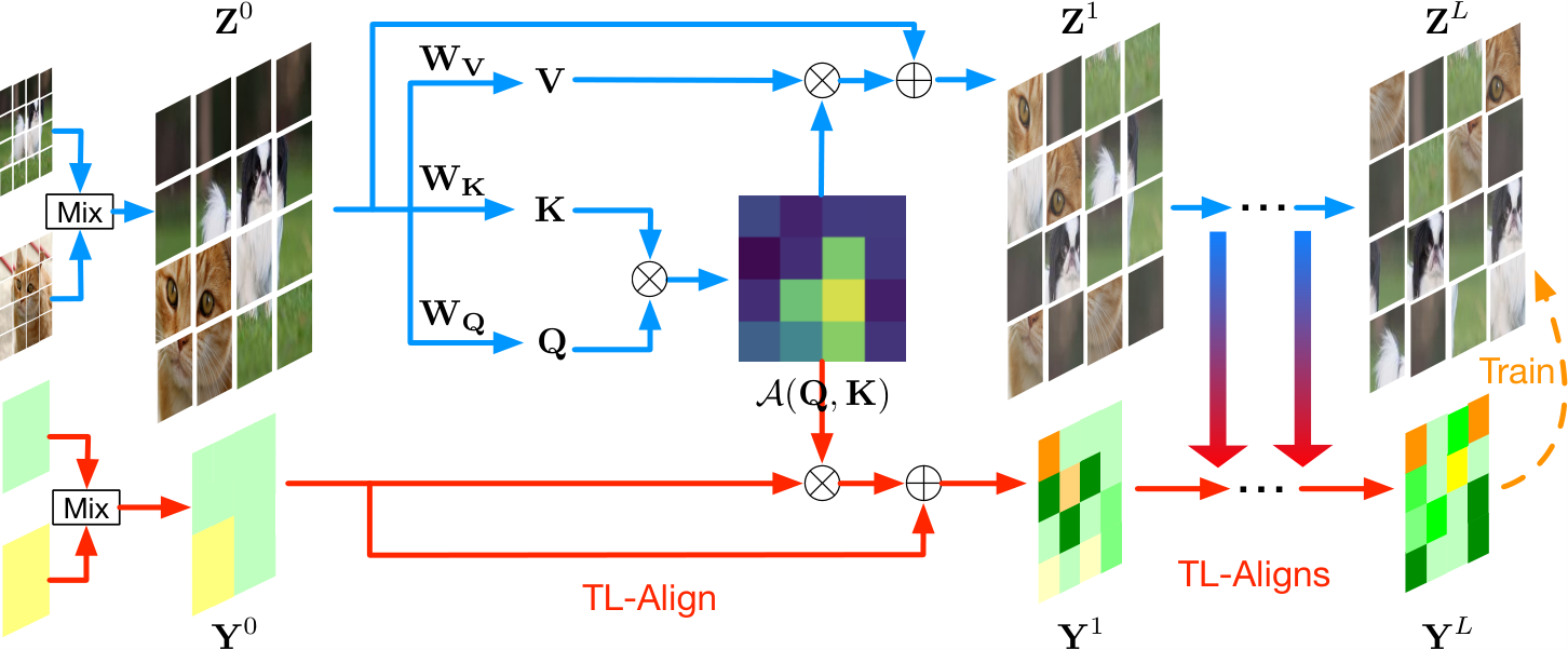
To address this, we propose a token-label alignment (TL-Align) method for ViTs to obtain a more accurate target for training. We present an overview of our method in Figure 1. We first assign a label to each input token in the mixed image according to the source of the token. We then trace the correspondence between the input tokens and the transformed tokens and align the labels accordingly. We assume that only the spatial self-attention and residual connection operation alter the presence of input tokens since channel MLP and layer normalization process each token independently. We reuse the computed attentions to linearly mix the labels of input tokens to obtain those of transformed tokens. The token-label alignment is performed iteratively to obtain a label for each output token. For class-token-based classification (e.g., ViT dosovitskiy2020image and DeiT touvron2021training), we directly use the aligned label for the output class token as the training target. For global-pooling-based classification (e.g., Swin liu2021swin), we similarly average the labels of output tokens as the training target. The proposed TL-Align is only used for training to improve performance and introduces no additional workload for inference. We apply the proposed TL-Align to various ViT variants with CutMix including plain ViTs (DeiT touvron2021training) and hierarchical ViTs (Swin liu2021swin). We observe a consistent performance boost across different models on ImageNet-1K deng2009imagenet. Specifically, our TL-Align improves DeiT-S by 0.8% using the same training recipe. We evaluate the ImageNet-pretrained models on various downstream tasks including semantic segmentation, objection detection, and transfer learning. Experimental results also verify the robustness and generalization ability of our method.
2 Related Work
Vision Transformer. Transformers have been widely used in natural language processing and achieved great success on many language tasks. Recently, Vision Transformers (ViTs) have aroused extensive interest in computer vision due to their competitive performance compared with CNNs dosovitskiy2020image; touvron2021training; liu2021swin; chu2021twins. Dosovitskiy et al. dosovitskiy2020image firstly introduced transformers into the image classification task. They split the input image into non-overlapped patches and then feed them into the transformer encoders. Liu et al. liu2021swin proposed a shifted windowing scheme to produce hierarchical feature maps suitable for dense prediction tasks. The great potential of vision transformer has motivated its adaptation to many challenging tasks including object detection dai2021dynamic; zhu2020deformable; carion2020end, segmentation cheng2021per; strudel2021segmenter, image enhancement chen2021pre; li2021efficient and video understanding liu2021video; arnab2021vivit.
Recently, some efforts have been devoted to producing better training targets to improve the performance of vision transformers jiang2021all; touvron2022deit. For example, DeiT touvron2021training introduces a knowledge distillation procedure to reduce the training cost of ViTs and achieves a better accuracy/speed trade-off. TokenLabeling jiang2021all employs a pretrained teacher annotator to predict a label for each token for dense knowledge distillation. Differently, we do not require a pretrained network to obtain the training targets. Our TL-Align maintains an aligned label for each token layer by layer and can be trained efficiently in an end-to-end manner.
Data Mixing Strategy. As an important type of data augmentation, data mixing strategies have demonstrated a consistent improvement in the generalization performance of CNNs. Zhang et al. zhang2018mixup first proposed to combine a training pair to create augmented samples for model regularization. They perform linear interpolations on both the input images and associated targets. Following MixUp, CutMix yun2019cutmix also utilizes the mixture of two input images but adopts a region copy-and-paste operation. Later methods including Puzzle Mix kim2020puzzle, SaliencyMix uddin2020saliencymix and Attentive CutMix walawalkar2020attentive leverage the salient regions for informative mixture generation. Recently, Yang et al. yang2022recursivemix proposed a RecursiveMix strategy which employs the historical input-prediction-label triplets for scale-invariant feature learning. Despite the better performance, a drawback of these methods is the heavily increased training cost due to the saliency extraction or historical information exploitation.
Most existing data mixing methods are originally designed for CNNs, and their effectiveness on ViTs has not been well explored. TransMix chen2021transmix uses the class attention map at the last layer to re-weight the mixing targets and assumes the output tokens to keep spatial correspondence with the input tokens. However, we identify a token fluctuation phenomenon for ViTs which may cause a mismatch between tokens and labels, leading to inaccurate label assignments in both the original CutMix and TransMix. To address this, we propose to align the label and token space by tracing their correspondence in a layerwise manner.
3 Proposed Approach
3.1 Preliminaries
The convolution neural network (CNN) has been the dominant architecture for computer vision in the deep learning era, greatly improving the performance of many tasks. Its monopoly has been challenged by the recent emergence of vision transformers (ViTs), which first “patchify” each image into tokens and process them with alternating self-attention (SA) and multi-layer perceptron (MLP).
In addition to architecture design, training strategy also has a large effect on the model performance, especially the data augmentation strategy. Data mixing walawalkar2020attentive; uddin2020saliencymix; kim2020puzzle; verma2019manifold; yun2019cutmix; zhang2018mixup is an important set of data augmentation for the training of both CNNs and ViTs, as it significantly improves the generalization ability of models. As the most commonly used data mixing strategy, CutMix yun2019cutmix aims to create virtual training samples from the given training samples , where denotes the input image and is the corresponding label. CutMix randomly selects a local region from one input and uses it to replace the pixels in the same region of another input to generate a new sample . Similarly, the label of is also the combination of the original labels and :
| (1) | ||||
where is a binary mask indicating the image each pixel belongs to, is an all-one matrix, and is the element-wise multiplication. reflects the mixing ratio of two labels and is the proportion of pixels cropped from in the mixed image . For a cropped region from , we compute to obtain the initial mixed target .
3.2 The Token Fluctuation Phenomenon
CutMix is originally designed for CNNs and assumes the feature extraction process does not alter the mixing ratio. However, we discover that different from CNNs, self-attention in ViTs can lead to the fluctuation of some tokens. The fluctuation further results in the mismatch between the token space and label space, which hinders the effective training of the network.
Formally, we use to denote a token of the image , i.e., is the transposed -th column vector of . We can then compute the -th transformed token after the spatial operation as , where is the -th element of the computed spatial mixing matrix .
With the assumption of the linear information integration, we define the contribution of an original token to a mixed token as where denotes the absolute value. We can then compute the presence of a token in all the mixed image tokens as:
| (2) |
For non-strided depth-wise convolution, each token is multiplied by each element in the convolutional kernel due to the translation invariance. We can thus obtain:
| (3) |
where denotes the set of positions that are not at the edge of the image, denotes the value of the -th position of the convolution kernel and is the kernel size. We can infer that , i.e., the effect of all the internal tokens does not change during the convolution process. However, for self-attention in ViTs, Eq. 3 does not hold due to the non-existence of translation invariance. The fluctuation of is further amplified by the input dependency of the spatial mixing matrix induced by self-attention. As an extreme case, we may obtain for certain tokens. The fluctuation of tokens will alter the proportion of mixing (i.e., ) and the network might even completely ignore one of the mixed images. The actual label of the processed tokens can then deviate from the mixed label computed by Eq. 1, resulting in less effective training.
3.3 Token-Label Alignment
Each token in ViTs interacts with other tokens using the self-attention mechanism. The input-dependent weights empower ViTs with more flexibility but also result in a mismatch between the processed token and the initial token. To address this, we propose a token-label alignment (TL-Align) method to trace the correspondence between the input and transformed tokens to obtain the aligned labels for the resulting representations, as illustrated in Figure 2.
Specifically, ViTs first split the mixed input after CutMix Eq. 1 to a sequence of non-overlapped patches and then flatten them to obtain the original image tokens . We then project them into a proper dimension and add positional embeddings:
| (4) |
where denotes the class token, N is the number of tokens, represents the patch projector, and is the position embeddings. Note that we adopt the process of the original transformer architecture dosovitskiy2020image as an example without loss of generality. Other models may omit the class token and use a relative positional embedding instead, which does not affect the utility of the proposed TL-Align method.
We first assign each token with a label embedding :
| (5) |
where the sum of elements in each equals 1 (i.e., ) and indicates how much the -th token belong to the -th class. We initialize the label embedding following the conventional data mixing paradigm. For example, when using CutMix to mix two images and from the -th class and the -th class with a mixing ratio of , we set and for the class token. For each patch token, we set if it comes from and if it comes from . If a patch token contains both the mixed images, we use the mixing ratio within this patch as the label. For MixUp, we can simply set all label embeddings with and .
We perform TL-Align in a layer-wise manner and compute the aligned labels based on the operation on the tokens. Formally, ViTs use self-attention to perform spatial mixing of the input tokens :
| (6) | ||||
To align the labels, we update the label embeddings using the same attention matrix :
| (7) |
ViTs usually adopt multi-head self-attention (MSA) to perform multiple self-attentions parallelly:
| (8) |
where is the number of heads and . We then adapt our label alignment to MSA by simply taking the average of all the attention matrices for alignment:
| (9) |
where is the attention matrix corresponding to the -th head .
Each transformer block processes the tokens by both spatial and channel mixing:
| (10) | ||||
where MLP and LN denote the MLP module and layer normalization ba2016layer, respectively. Our TL-Align then aligns the label embeddings in a similar manner:
| (11) | ||||
where Norm denotes the normalization operation. We implement Norm by a simple average.
Hierarchical vision transformers such as Swin liu2021swin further introduce a patch aggregation operation to merge multiple patches. They usually concatenate multiple tokens across the channels to reduce the spatial resolution. Instead of concatenation, we simply add the label embeddings of the merged tokens followed by normalization as the aligned labels. The proposed TL-Align can be generalized to different architectures composed of spatial mixing, channel mixing, point-wise transformation, residual connection, and spatial aggregation. We provide detailed illustrations of alignment with these operations in the appendix.
We synchronously align the labels with the processed tokens layer by layer and obtain the aligned tokens and labels . The final representation of the image is either the class token dosovitskiy2020image; touvron2021training or the average pooling of all the spatial tokens liu2021swin. The aligned label for the image is then or depending on the specific model. We then adopt the aligned label to train the network and can adapt to different loss functions and training schemes:
| (12) |
We do not back-propagate through the aligned label as they only serve as a more accurate target.
Our TL-Align serves as a plug-and-play module on various vision transformers while only introducing negligible training costs. We adjust the label of each token adaptively during the layer-by-layer propagation and preserve alignment between tokens and labels throughout the forward process. TL-Align is only used during training and introduces no additional computation cost when inference.
4 Experiments
In this section, we conducted extensive experiments to evaluate the proposed TL-Align method. We demonstrate the improvement of TL-Align on various vision transformers and compare it with state-of-the-art training strategies concerning accuracy, network complexity, and training speed. We examine the transferability on downstream tasks including semantic segmentation, object detection, and transfer learning. We further provide in-depth analysis to evaluate the effectiveness of TL-Align.
| Model | Image Size | Params | FLOPs | Top-1(%) | Top-5(%) |
|---|---|---|---|---|---|
| DeiT-T | 5.7M | 1.6G | 72.2 | 91.3 | |
| +TL-Align | 73.2 | 91.7 | |||
| PVT-T | 13.2M | 1.9G | 75.1 | 92.4 | |
| +TL-Align | 75.5 | 93.0 | |||
| DeiT-S | 22M | 4.6G | 79.8 | 95.0 | |
| +TL-Align | 80.6 | 95.0 | |||
| PVT-S | 24.5M | 3.8G | 79.8 | 95.0 | |
| +TL-Align | 80.4 | 95.5 | |||
| Swin-T | 29M | 4.5G | 81.2 | 95.5 | |
| +TL-Align | 81.4 | 95.7 | |||
| Swin-S | 50M | 8.8G | 83.0 | 96.3 | |
| +TL-Align | 83.4 | 96.5 | |||
| DeiT-B | 86M | 17.5G | 81.8 | 95.5 | |
| +TL-Align | 82.3 | 95.8 | |||
| Swin-B | 88M | 15.4G | 83.5 | 96.4 | |
| +TL-Align | 83.7 | 96.5 |
| Method | Params | Speed (image/s) | Acc.(%) |
|---|---|---|---|
| Vanilla | 22M | 322 | 76.4 |
| CutMix | 22M | 322 | 79.8 |
| Puzzle-Mix | 22M | 139 | 79.8 |
| SaliencyMix | 22M | 314 | 79.2 |
| Attentive-CutMix | 46M | 239 | 77.5 |
| TransMix | 22M | 322 | 80.1 |
| CutMix + TL-Align | 22M | 311 | 80.6 |
| Backbone | Params | FLOPs | mIoU | mIoU (MS) | mAcc |
|---|---|---|---|---|---|
| DeiT-S | 58M | 1032G | 43.8 | 45.1 | 55.2 |
| +TL-Align | 44.5 | 45.7 | 55.5 | ||
| Swin-T | 60M | 945G | 44.4 | 45.8 | 55.6 |
| +TL-Align | 44.7 | 46.5 | 56.4 | ||
| Swin-S | 81M | 1038G | 47.6 | 49.5 | 58.8 |
| +TL-Align | 48.0 | 49.7 | 59.5 | ||
| Swin-B | 121M | 1188G | 48.1 | 49.7 | 59.1 |
| +TL-Align | 48.3 | 50.1 | 59.7 |
4.1 ImageNet Classification
Implementation Details. We first evaluate TL-Align on ImageNet russakovsky2015imagenet for image classification. ImageNet russakovsky2015imagenet contains 1.2M training images and 50K validation images from 1K categories and is a widely-used benchmark for performance evaluation. We implement our method based on PyTorch paszke2019pytorch and the timm library rw2019timm. We conduct experiments on various transformer architectures: three variants of DeiT touvron2021training (DeiT-T, DeiT-S, and DeiT-B), two variants of PVT wang2021pyramid (PVT-T, PVT-S) and three variants of Swin Transformer liu2021swin (Swin-T, Swin-S, and Swin-B). For tiny and small models, we train from scratch for 300 epochs following the same training recipe using CutMix as DeiT touvron2021training, PVT wang2021pyramid and Swin liu2021swin. We keep all the data augmentation policies and all hyperparameter settings unchanged for fair comparisons. The only modification is that we replace the mixing targets in CutMiX with the labels obtained by our TL-Align. For base models (i.e., Deit-B and Swin-B), we finetune the official pre-trained models for 40 epochs with a constant learning rate of 1e-5 and a weight decay of 1e-8.
| o 0.8l—*3X[c]—*3X[c]—*3X[c] Backbone | Params | FLOPs | Schedule | ||||||
|---|---|---|---|---|---|---|---|---|---|
| Swin-T | 86M | 745G | 3x | 50.4 | 69.2 | 54.7 | 43.7 | 66.6 | 47.3 |
| +TL-Align | 50.5 | 69.4 | 54.9 | 43.8 | 66.6 | 47.3 | |||
| Swin-S | 107M | 838G | 3x | 51.9 | 70.7 | 56.3 | 45.0 | 68.2 | 48.8 |
| +TL-Align | 52.2 | 71.1 | 56.7 | 45.2 | 68.4 | 49.1 | |||
| Swin-B | 145M | 982G | 3x | 51.9 | 70.5 | 56.4 | 45.0 | 68.1 | 48.9 |
| +TL-Align | 52.3 | 71.2 | 56.9 | 45.3 | 68.7 | 49.1 |
| Model | Params | FLOPs | C-10 | C-100 | Flowers | Cars |
|---|---|---|---|---|---|---|
| ResNet50 | 26M | 4.1G | - | - | 96.2 | 90.0 |
| ViT-B/16 | 86M | 55.4G | 98.1 | 87.1 | 89.5 | - |
| ViT-L/16 | 307M | 190.7G | 97.9 | 86.4 | 89.7 | - |
| Deit-T | 5.7M | 1.6G | 97.6 | 85.7 | 97.1 | 90.1 |
| +TL-Align | 5.7M | 1.6G | 97.8 | 86.4 | 97.9 | 90.7 |
| Deit-S | 22M | 4.6G | 97.9 | 90.2 | 98.1 | 91.4 |
| +TL-Align | 22M | 4.6G | 98.8 | 90.4 | 98.3 | 91.8 |
| Deit-B | 86M | 17.5G | 99.1 | 90.8 | 98.4 | 92.1 |
| +TL-Align | 86M | 17.5G | 99.1 | 90.5 | 98.6 | 93.0 |
Performance on Different Architectures. As shown in Table 1, TL-Align steadily improves the performance of different vision transformer architectures. Specifically, TL-Align boosts the top-1 accuracy of DeiT-T, DeiT-S, and DeiT-B by 1.0%, 0.8%, and 0.5%, respectively, in a parameter-free manner. Moreover, our method is generalizable and can be directly applied to hierarchical vision transformers like Swin. It is worth noting that most existing methods need either architecture modifications (adding a class token in chen2021transmix) or extra computations (saliency map extraction in uddin2020saliencymix) when applied to Swin. In contrast, our TL-Align method can be used as a plug-and-play module and achieves consistent improvement on variants of Swin.
| Model | FLOPs | Params | ImageNet | Generalization | Robustness | ||||
|---|---|---|---|---|---|---|---|---|---|
| Top-1 | Top-5 | IN-V2 | IN-A | IN-C | IN-R | AutoAttack | |||
| DeiT-T | 5.7M | 1.6G | 72.2 | 91.3 | 60.4 | 7.7 | 69.1 | 34.1 | 3.9 |
| +TL-Align | 5.7M | 1.6G | 73.2 | 91.7 | 61.4 | 6.1 | 68.0 | 34.6 | 4.4 |
| DeiT-S | 22M | 4.6G | 79.8 | 95.0 | 68.5 | 18.9 | 54.7 | 42.5 | 6.9 |
| +TL-Align | 22M | 4.6G | 80.6 | 95.0 | 68.9 | 19.2 | 53.2 | 43.2 | 7.5 |
| DeiT-B | 86M | 17.5G | 81.8 | 95.5 | 70.5 | 27.9 | 48.5 | 45.3 | - |
| +TL-Align | 86M | 17.5G | 82.3 | 95.8 | 70.9 | 29.0 | 47.1 | 44.4 | - |
| MixUp | CutMix | Random | Block-wise | Top-1 (%) | +TL-Align |
|---|---|---|---|---|---|
| Top-1 (%) | |||||
| 76.4 | - | ||||
| 79.8 | 80.6 | ||||
| 79.8 | 80.2 | ||||
| 79.7 | 80.2 | ||||
| 80.0 | 80.3 |
Comparison with Other Training Strategies. We also compare our method with the state-of-the-art training strategies for data mixing on DeiT-S, including CutMix yun2019cutmix, Puzzle-Mix kim2020puzzle, SaliencyMix uddin2020saliencymix, Attentive-CutMix walawalkar2020attentive, and TransMix chen2021transmix. Specifically, we train the DeiT-S model while only disabling CutMix as the baseline method, which is denoted as Vanilla in Table 2. Moreover, since TransMix chen2021transmix reports the EMA accuracy with different hyperparameters, we reproduce it under the same training recipe touvron2021training for a fair comparison. As demonstrated in Table 2, TL-Align shows significantly better performance than the other mixup variants while maintaining the number of parameters and training speed. Puzzle-Mix obtains the same classification accuracy as CutMix but results in a much lower training speed as it relies on an extra model to get the optimal solution. SaliencyMix and Attentive-CutMix lead to performance degeneration when built upon DeiT-S backbone. Notably, our method also achieves higher top-1 accuracy than ViT-targeted TransMix. Due to the token fluctuation phenomenon, the class token attention utilization in TransMix can not reflect the actual contribution of different tokens. Differently, TL-Align obtains accurate alignment of the tokens and labels, resulting in improved performance.
4.2 Downstream Tasks
Semantic Segmentation. We evaluate our TL-Align on ADE20K dataset zhou2019semantic for semantic segmentation. ADE20K zhou2019semantic contains 20K training images and 2K validation images from 150 semantic categories. We adopt DeiT-S and three variants of Swin Transformer as backbones equipped with UpperNet for segmentation. As presented in Table 3, TL-Align improves the segmentation performance on both DeiT and Swin at different model scales.
Object Detection and Instance Segmentation. We also examine the performance of TL-Align on object detection and instance segmentation on the COCO 2017 dataset lin2014microsoft, which consists of 118K training images and 5K validation images from 80 categories. We apply our TL-Align to Swin liu2021swin due to the advantage of the hierarchical representations on object detection tasks. We adopt the Cascade Mask-RCNN cai2018cascade framework and use the training strategy of 3x schedule. As shown in Table 4, we observe consistent improvements on all variants of Swin Transformer. This demonstrates the advantages to learn token-level meaningful features suitable for dense prediction tasks.
Transfer Learning. We further evaluate the transferred classification performance of TL-Align on CIFAR-10 krizhevsky2009learning, CIFAR-100 krizhevsky2009learning, Flowers nilsback2008automated and Cars krause20133d. We use pre-trained models on ImageNet and finetune them on these datasets following existing works touvron2021training. We compare the performance with and without TL-Align on three variants of DeiT touvron2021training, as shown in Table 5. TL-Align obtains significant performance gains for all variants on the four datasets.
4.3 Performance Analysis and Visualization
Effectiveness of Token-Label Alignment. We first quantize the difference between the original targets and aligned labels and investigate its correlation with the model. Specifically, we compute the Root Mean Square Error (RMSE) between the original targets and labels obtained by our TL-Align. As shown in Figure 3, the RMSE decreases when enlarging the model size. This indicates that larger models demonstrates less token fluctuation since the self-correction ability is also enhanced as the model capacity scales up. Moreover, the RMSE for Swin Transformer tends to be lower compared with DeiT of similar model size. This is due to the local-window self-attention in Swin which preserves more local information. These observations are consistent with our experimental results: the improvements on small models and DeiT-like backbones tend to be more significant as they encounter more token fluctuation.
Visualization of the Layer-wise Mixing Ratio of Fluctuated Tokens. To investigate the effectiveness of TL-Align, we compute a similarity-based “ground-truth” mixing ratio for each layer. Specifically, we compute the similarities of tokens between the mixed and unmixed images and use them as the label of each token. We compare them with the mixing ratios produced by TL-Align, CutMix yun2019cutmix, TransMix chen2021transmix, and TokenLabeling jiang2021all. As shown in Figure 4, the similarity-based mixing ratio changes at each layer, resulting from token fluctuation. However, CutMix, TransMix, and TokenLabeling assume the output tokens keep spatial correspondence with the input tokens and compute a fixed mixing ratio. TL-Align assigns dynamic labels to tokens using layer-wise alignment, which is more accurate compared with other methods.
| Alignment | Top-1 Acc.(%) | (%) |
|---|---|---|
| None (DeiT-S baseline) | 79.8 | - |
| TL-Align-S (Layer 12) | 80.1 | +0.3 |
| TL-Align-S (Layer 2,4,6,8) | 80.2 | +0.4 |
| Normalization Disabled | 80.3 | +0.5 |
| Default (TL-Align) | 80.6 | +0.8 |

Evaluation of Robustness and Generalization. We further conduct experiments to validate the generalization and robustness of TL-Align, as shown in Table 6. We employ four corrupted and out-of-distribution datasets for robustness evaluation. ImageNet-Ahendrycks2021natural consists of naturally adversarial examples from real-world challenging scenarios. ImageNet-C hendrycks2019benchmarking is used to evaluate model robustness to diverse image corruptions. ImageNet-R hendrycks2021many contains various artistic renditions of 200 ImageNet classes. We also adopt AutoAttack croce2020reliable to evaluate the adversarial robustness on the ImageNet validation set. Due to memory limitation, we do not experiment with DeiT-B on AutoAttack. We use mean Corruption Error (mCE) for ImageNet-C and Top-1 Accuracy for others as the evaluation metric. For generalization evaluation, we adopt the ImageNet-V2 dataset recht2019imagenet which contains new test sets of ImageNet following the same labeling protocol. We see that TL-Align improves both robustness and generalization, showing the superiority of adopting TL-Align for pre-training.
Ablation Study on different Data Mixing Strategies. Due to the efficiency of the proposed layer-wise alignment, TL-Align can be directly applied to a wide range of data mixing strategies. We adopt MixUp, CutMix, a random mixing strategy and a block-wise mixing strategy to evaluate the generalizability of TL-Align. The random mixing and block-wise mixing strategies are inspired by MAE he2022masked and BEiT bao2021beit and we replace the masking operation with image mixing on patch-level and block-level (both of size 1616) respectively. The comparison results of training DeiT-S with and without our approach is demonstrated in Table 7. Specifically, TL-Align improves CutMix by 0.8%, MixUp+CutMix by 0.4%, random mixing by 0.5% and block-wise mixing by 0.3% respectively, further verifying the generalizability of the proposed TL-Align.
Ablation Study on Different Label Alignment Operations. Our TL-Align aligns the labels with tokens transformed by spatial self-attention and residual connection layer-by-layer. To investigate the effect of reusing attention maps and normalization, we conduct an ablation study regarding different alignment operations on DeiT-S. We try aligning the labels only by using the attention map of Layer 12, which is equivalent to TransMix chen2021transmix. We also test the performance of applying alignment to several middle transformer layers and disabling normalization. As presented in Table 8, incomplete alignment at a part of layers marginally boosts the performance as it cannot well handle the token fluctuation issue. Disabling normalization leads to 0.3 accuracy drop due to the inaccurate alignment at the presence of residual connections. This demonstrates the significance of the token-label alignment by attention utilization and normalization in a layer-wise manner.
Visualizations of Aligned Labels. We visualize the labels obtained by TL-Align on DeiT-S touvron2021training and Swin-S liu2021swin as shown in Figure 5. Specifically, the aligned label embedding is obtained after the final transformer block for both DeiT-S and Swin-S. The value of the label embedding represents the probability of the belonged class of the corresponding token. We use red to denote larger probabilities towards the first image and blue for the second image. We observe that the aligned labels can deviate from the original labels and result in different mixing ratios for training. Therefore, using the original ratio as the training target may produce false training signals and lead to inferior performance. We see that TL-Align can correct the labels when the images are mixed with uninformative tokens. More visualization results are included in the appendix.
5 Conclusion
In this paper, we have presented a token-label alignment method for training better vision transformers. As important subsets of data augmentation methods, data mixing strategies can generally improve the performance of both CNNs and ViTs. We identify a token fading issue for ViTs and address it by tracing the correspondence between transformed tokens and the original tokens to obtain a label for each output token to obtain more accurate training signals. Experimental results have demonstrated that our TL-Align can consistently improve the performance of various ViT models. The generalization performance of TL-Align to other architectures such as MLP-like models remains unknown and is a promising future direction to explore.
Appendix A Comparisons of Different Training Recipes
We compare different training recipes for the DeiT-S model in Table 9. The results of TransMix chen2021transmix reported in the original paper adopts an advanced training recipe with a model exponential moving average, resulting in slower training speed. Differently, we basically follow the conventional DeiT-S touvron2021training training recipe and improve its performance by 0.8%. We report the result of TransMix with the same training recipe (80.1%) in Table 2.
| Method | Training | Warmup | LR | Weight | Model | EMA | MixUp | CutMix | MixUp | Random | Top-1 |
|---|---|---|---|---|---|---|---|---|---|---|---|
| Epochs | Epochs | Decay | EMA | Decay | Switch Prob | Erasing | Acc. (%) | ||||
| DeiT-S1 touvron2021training | 300 | 5 | 0.0005 | 0.05 | - | 0.0 | 0.0 | - | 76.4 | ||
| DeiT-S2 touvron2021training | 300 | 5 | 0.0005 | 0.05 | - | 0.8 | 1.0 | 0.5 | 79.8 | ||
| DeiT-S3 touvron2021training | 310 | 20 | 0.001 | 0.03 | 0.99996 | 0.8 | 1.0 | 0.8 | 80.3 | ||
| +TransMix chen2021transmix | 310 | 20 | 0.001 | 0.03 | 0.99996 | 0.8 | 1.0 | 0.8 | 80.7 (+0.4) | ||
| DeiT-S4 touvron2021training | 300 | 5 | 0.0005 | 0.05 | - | 0.0 | 1.0 | - | 79.8 | ||
| +TransMix chen2021transmix | 300 | 5 | 0.0005 | 0.05 | - | 0.0 | 1.0 | - | 80.1 (+0.3) | ||
| +TL-Align | 300 | 5 | 0.0005 | 0.05 | - | 0.0 | 1.0 | - | 80.6 (+0.8) |
Appendix B Details of Experimental Analysis
Obtaining the “Ground-truth” Mixing Ratio.
To better demonstrate the token fluctuation phenomenon, we compute a “ground-truth” mixing ratio based on token similarity as shown in Figure 6. Formally, given two input images , and their mixed sample generated by CutMix, we feed all of them into the vision transformer obtain get the corresponding tokens , and after the transformer block . For each mixed token in , we compute its maximum cosine similarity with all tokens in and :
| (13) | |||
The contribution of input to the token is then obtained using the softmax function: . We visualize this similarity-based mixing ratio of the class token in DeiT-S in Figure 4. The token mixing ratio changes after each transformer block’s processing, demonstrating the token fluctuation problem. Moreover, TL-Align assigns a dynamic mixing ratio to tokens at different layers, which is more consistent with the “ground truth” compared with other methods. This provides an empirical analysis to explain the improvement achieved by our TL-Align.

Implementation of Different Data Mixing Strategies.
We provide implementation details of different data mixing strategies that we adopt to evaluate the effectiveness of TL-Align. Inspired by MAE he2022masked and BEiT bao2021beit, we implement a random mixing strategy and block-wise mixing strategy. The visualization of the mixed images produced by CutMix, random mixing, and block-wise mixing strategies is shown in Figure 7. Specifically, employing the block-wise strategy leads to the highest top-1 accuracy of . Our TL-Align further boosts the accuracy by , verifying its generalizability on various data mixing strategies.

Appendix C More Visualization Results
We provide more visualization results of the obtained labels by the proposed token-label alignment method in Figure 8. We visualize the input images, the mixed image, the original label embedding, and the label embedding after our TL-Align. Specifically, we visualize the aligned label embedding after the final transformer block for both DeiT-S and Swin-S. The size of the original label embedding is equivalent to the number of input tokens, i.e., for DeiT-S and for Swin-Transformer since they employ different patch sizes for patch embedding. The value of the label embedding represents the probability of which class the corresponding token belongs to, which is shown by color. Red stands for the class of the first input image while blue stands for the class of the second input image. We observe that the aligned labels can deviate from the original labels, resulting in different mixing ratios during training. Therefore, using the original mixing ratio as the training target produces false training signals and might lead to inferior performance.

Appendix D Generalizing TL-Align Beyond ViTs
ViTs can achieve better accuracy/computation trade-off than conventional CNNs, where one of the working mechanisms is the alternation between spatial mixing (e.g., SA) and channel mixing (e.g., MLP) tolstikhin2021mlp. Based on this, some works have explored different spatial mixing strategies in addition to self-attention, including spatial MLP tolstikhin2021mlp; touvron2021resmlp; tang2021image; wei2022activemlp and depth-wise convolution ding2022scaling; liu2022convnet; guo2022visual. For an image , they first perform patch-wise image tokenization to obtain a tokenized image representation , where is the number of tokens and is the number of channels. To generalize TL-Align to other architectures beyond ViTs, we first formulate modern deep vision networks into various compositions of five operations:
- •
Spatial mixing: , where .
- •
Channel mixing: , where .
- •
Point-wise transformation: , where is a point-wise operation such as bias adding and normalization.
- •
Residual connection: , where can be one or a composition of the aforementioned operations.
- •
Spatial aggregation: , where Aggre typically concatenates multiple tokens across the feature dimension.
For example, MLP-Mixer tolstikhin2021mlp adopts , where is a learnable parameter matrix. ConvNeXt liu2022convnet adopts , where is a convolutional kernel and transforms the kernel into a equivalent matrix for direct multiplication.
The proposed TL-Align can be generalized to different architectures by applying the corresponding operations on the label embeddings. We initialize the label embedding following (5). We detail the label embedding updating for different operations in Table 10. The operation denotes that we normalize each row vector so that the sum of all elements equals to 1.
| Operation | Token Processing | Label Alignment | Example |
|---|---|---|---|
| Spatial mixing | Spatial attention | ||
| Channel mixing | Channel MLP | ||
| Point-wise transformation | Layer normalization | ||
| Residual connection | Residual connection | ||
| Spatial aggregation | Patch merging |
For spatial mixing, we accordingly mix the token embeddings using the same weights as the token processing. For example, for a processed token , we similarly compute the aligned label as , assuming the label information is linearly addable. As channel mixing and point-wise transformation only reorganize information within each token, they do not alter the label embedding. For residual connection, we similarly add a residual connection to the label embedding before normalization. Spatial aggregation is similar to spatial mixing and also aggregates information among multiple tokens. Therefore, we also need to align the labels by adding their label embeddings before normalization. We leave the experiments for generalized TL-Align for future works.
References
- (1) Anurag Arnab, Mostafa Dehghani, Georg Heigold, Chen Sun, Mario Lučić, and Cordelia Schmid. Vivit: A video vision transformer. In ICCV, pages 6836–6846, 2021.
- (2) Jimmy Lei Ba, Jamie Ryan Kiros, and Geoffrey E Hinton. Layer normalization. arXiv, abs/1607.06450, 2016.
- (3) Hangbo Bao, Li Dong, and Furu Wei. Beit: Bert pre-training of image transformers. arXiv preprint arXiv:2106.08254, 2021.
- (4) Zhaowei Cai and Nuno Vasconcelos. Cascade r-cnn: Delving into high quality object detection. In CVPR, pages 6154–6162, 2018.
- (5) Nicolas Carion, Francisco Massa, Gabriel Synnaeve, Nicolas Usunier, Alexander Kirillov, and Sergey Zagoruyko. End-to-end object detection with transformers. In ECCV, pages 213–229, 2020.
- (6) Hanting Chen, Yunhe Wang, Tianyu Guo, Chang Xu, Yiping Deng, Zhenhua Liu, Siwei Ma, Chunjing Xu, Chao Xu, and Wen Gao. Pre-trained image processing transformer. In CVPR, pages 12299–12310, 2021.
- (7) Jie-Neng Chen, Shuyang Sun, Ju He, Philip Torr, Alan Yuille, and Song Bai. Transmix: Attend to mix for vision transformers. arXiv preprint arXiv:2111.09833, 2021.
- (8) Tianlong Chen, Zhenyu Zhang, Yu Cheng, Ahmed Awadallah, and Zhangyang Wang. The principle of diversity: Training stronger vision transformers calls for reducing all levels of redundancy. In CVPR, 2022.
- (9) Bowen Cheng, Alexander G Schwing, and Alexander Kirillov. Per-pixel classification is not all you need for semantic segmentation. In NeurIPS, 2021.
- (10) Xiangxiang Chu, Zhi Tian, Yuqing Wang, Bo Zhang, Haibing Ren, Xiaolin Wei, Huaxia Xia, and Chunhua Shen. Twins: Revisiting the design of spatial attention in vision transformers. In NeurIPS, 2021.
- (11) Francesco Croce and Matthias Hein. Reliable evaluation of adversarial robustness with an ensemble of diverse parameter-free attacks. In International conference on machine learning, pages 2206–2216. PMLR, 2020.
- (12) Xiyang Dai, Yinpeng Chen, Jianwei Yang, Pengchuan Zhang, Lu Yuan, and Lei Zhang. Dynamic detr: End-to-end object detection with dynamic attention. In ICCV, pages 2988–2997, 2021.
- (13) Zhigang Dai, Bolun Cai, Yugeng Lin, and Junying Chen. Up-detr: Unsupervised pre-training for object detection with transformers. In CVPR, pages 1601–1610, 2021.
- (14) Jia Deng, Wei Dong, Richard Socher, Li-Jia Li, Kai Li, and Li Fei-Fei. Imagenet: A large-scale hierarchical image database. In CVPR, pages 248–255. Ieee, 2009.
- (15) Xiaohan Ding, Xiangyu Zhang, Yizhuang Zhou, Jungong Han, Guiguang Ding, and Jian Sun. Scaling up your kernels to 31x31: Revisiting large kernel design in cnns. In CVPR, 2022.
- (16) Alexey Dosovitskiy, Lucas Beyer, Alexander Kolesnikov, Dirk Weissenborn, Xiaohua Zhai, Thomas Unterthiner, Mostafa Dehghani, Matthias Minderer, Georg Heigold, Sylvain Gelly, et al. An image is worth 16x16 words: Transformers for image recognition at scale. In ICLR, 2020.
- (17) Meng-Hao Guo, Cheng-Ze Lu, Zheng-Ning Liu, Ming-Ming Cheng, and Shi-Min Hu. Visual attention network. arXiv preprint arXiv:2202.09741, 2022.
- (18) Kaiming He, Xinlei Chen, Saining Xie, Yanghao Li, Piotr Dollár, and Ross Girshick. Masked autoencoders are scalable vision learners. In Proceedings of the IEEE/CVF Conference on Computer Vision and Pattern Recognition, pages 16000–16009, 2022.
- (19) Dan Hendrycks, Steven Basart, Norman Mu, Saurav Kadavath, Frank Wang, Evan Dorundo, Rahul Desai, Tyler Zhu, Samyak Parajuli, Mike Guo, et al. The many faces of robustness: A critical analysis of out-of-distribution generalization. In Proceedings of the IEEE/CVF International Conference on Computer Vision, pages 8340–8349, 2021.
- (20) Dan Hendrycks and Thomas Dietterich. Benchmarking neural network robustness to common corruptions and perturbations. arXiv preprint arXiv:1903.12261, 2019.
- (21) Dan Hendrycks, Kevin Zhao, Steven Basart, Jacob Steinhardt, and Dawn Song. Natural adversarial examples. In Proceedings of the IEEE/CVF Conference on Computer Vision and Pattern Recognition, pages 15262–15271, 2021.
- (22) Zi-Hang Jiang, Qibin Hou, Li Yuan, Daquan Zhou, Yujun Shi, Xiaojie Jin, Anran Wang, and Jiashi Feng. All tokens matter: Token labeling for training better vision transformers. In NeurIPS, 2021.
- (23) Jang-Hyun Kim, Wonho Choo, and Hyun Oh Song. Puzzle mix: Exploiting saliency and local statistics for optimal mixup. In ICML, pages 5275–5285, 2020.
- (24) Jonathan Krause, Michael Stark, Jia Deng, and Li Fei-Fei. 3d object representations for fine-grained categorization. In ICCVW, pages 554–561, 2013.
- (25) Alex Krizhevsky, Geoffrey Hinton, et al. Learning multiple layers of features from tiny images. 2009.
- (26) Wenbo Li, Xin Lu, Jiangbo Lu, Xiangyu Zhang, and Jiaya Jia. On efficient transformer and image pre-training for low-level vision. arXiv preprint arXiv:2112.10175, 2021.
- (27) Xiaoxiao Li, Ziwei Liu, Ping Luo, Chen Change Loy, and Xiaoou Tang. Not all pixels are equal: Difficulty-aware semantic segmentation via deep layer cascade. In CVPR, pages 3193–3202, 2017.
- (28) Tsung-Yi Lin, Michael Maire, Serge Belongie, James Hays, Pietro Perona, Deva Ramanan, Piotr Dollár, and C Lawrence Zitnick. Microsoft coco: Common objects in context. In ECCV, pages 740–755, 2014.
- (29) Ze Liu, Yutong Lin, Yue Cao, Han Hu, Yixuan Wei, Zheng Zhang, Stephen Lin, and Baining Guo. Swin transformer: Hierarchical vision transformer using shifted windows. In ICCV, 2021.
- (30) Zhuang Liu, Hanzi Mao, Chao-Yuan Wu, Christoph Feichtenhofer, Trevor Darrell, and Saining Xie. A convnet for the 2020s. arXiv preprint arXiv:2201.03545, 2022.
- (31) Ze Liu, Jia Ning, Yue Cao, Yixuan Wei, Zheng Zhang, Stephen Lin, and Han Hu. Video swin transformer. arXiv preprint arXiv:2106.13230, 2021.
- (32) Maria-Elena Nilsback and Andrew Zisserman. Automated flower classification over a large number of classes. In Indian Conference on Computer Vision, Graphics and Image Processing, 2008.
- (33) Adam Paszke, Sam Gross, Francisco Massa, Adam Lerer, James Bradbury, Gregory Chanan, Trevor Killeen, Zeming Lin, Natalia Gimelshein, Luca Antiga, et al. Pytorch: An imperative style, high-performance deep learning library. In NIPS, pages 8026–8037, 2019.
- (34) Benjamin Recht, Rebecca Roelofs, Ludwig Schmidt, and Vaishaal Shankar. Do imagenet classifiers generalize to imagenet? In International Conference on Machine Learning, pages 5389–5400. PMLR, 2019.
- (35) Olga Russakovsky, Jia Deng, Hao Su, Jonathan Krause, Sanjeev Satheesh, Sean Ma, Zhiheng Huang, Andrej Karpathy, Aditya Khosla, Michael Bernstein, et al. Imagenet large scale visual recognition challenge. IJCV, 115(3):211–252, 2015.
- (36) Robin Strudel, Ricardo Garcia, Ivan Laptev, and Cordelia Schmid. Segmenter: Transformer for semantic segmentation. In ICCV, 2021.
- (37) Yehui Tang, Kai Han, Jianyuan Guo, Chang Xu, Yanxi Li, Chao Xu, and Yunhe Wang. An image patch is a wave: Quantum inspired vision mlp. In CVPR, 2022.
- (38) Ilya O Tolstikhin, Neil Houlsby, Alexander Kolesnikov, Lucas Beyer, Xiaohua Zhai, Thomas Unterthiner, Jessica Yung, Andreas Steiner, Daniel Keysers, Jakob Uszkoreit, et al. Mlp-mixer: An all-mlp architecture for vision. NeurIPS, 34, 2021.
- (39) Hugo Touvron, Piotr Bojanowski, Mathilde Caron, Matthieu Cord, Alaaeldin El-Nouby, Edouard Grave, Gautier Izacard, Armand Joulin, Gabriel Synnaeve, Jakob Verbeek, et al. Resmlp: Feedforward networks for image classification with data-efficient training. arXiv preprint arXiv:2105.03404, 2021.
- (40) Hugo Touvron, Matthieu Cord, Matthijs Douze, Francisco Massa, Alexandre Sablayrolles, and Hervé Jégou. Training data-efficient image transformers & distillation through attention. In ICML, pages 10347–10357, 2021.
- (41) Hugo Touvron, Matthieu Cord, and Hervé Jégou. Deit iii: Revenge of the vit. arXiv preprint arXiv:2204.07118, 2022.
- (42) AFM Uddin, Mst Monira, Wheemyung Shin, TaeChoong Chung, Sung-Ho Bae, et al. Saliencymix: A saliency guided data augmentation strategy for better regularization. arXiv preprint arXiv:2006.01791, 2020.
- (43) Vikas Verma, Alex Lamb, Christopher Beckham, Amir Najafi, Ioannis Mitliagkas, David Lopez-Paz, and Yoshua Bengio. Manifold mixup: Better representations by interpolating hidden states. In ICML, pages 6438–6447, 2019.
- (44) Devesh Walawalkar, Zhiqiang Shen, Zechun Liu, and Marios Savvides. Attentive cutmix: An enhanced data augmentation approach for deep learning based image classification. arXiv preprint arXiv:2003.13048, 2020.
- (45) Wenhai Wang, Enze Xie, Xiang Li, Deng-Ping Fan, Kaitao Song, Ding Liang, Tong Lu, Ping Luo, and Ling Shao. Pyramid vision transformer: A versatile backbone for dense prediction without convolutions. In ICCV, 2021.
- (46) Guoqiang Wei, Zhizheng Zhang, Cuiling Lan, Yan Lu, and Zhibo Chen. Activemlp: An mlp-like architecture with active token mixer. arXiv preprint arXiv:2203.06108, 2022.
- (47) Ross Wightman. Pytorch image models. https://github.com/rwightman/pytorch-image-models, 2019.
- (48) Lingfeng Yang, Xiang Li, Borui Zhao, Renjie Song, and Jian Yang. Recursivemix: Mixed learning with history. arXiv preprint arXiv:2203.06844, 2022.
- (49) Sangdoo Yun, Dongyoon Han, Seong Joon Oh, Sanghyuk Chun, Junsuk Choe, and Youngjoon Yoo. Cutmix: Regularization strategy to train strong classifiers with localizable features. In ICCV, pages 6023–6032, 2019.
- (50) Hongyi Zhang, Moustapha Cisse, Yann N Dauphin, and David Lopez-Paz. mixup: Beyond empirical risk minimization. In ICLR, 2018.
- (51) Sixiao Zheng, Jiachen Lu, Hengshuang Zhao, Xiatian Zhu, Zekun Luo, Yabiao Wang, Yanwei Fu, Jianfeng Feng, Tao Xiang, Philip HS Torr, et al. Rethinking semantic segmentation from a sequence-to-sequence perspective with transformers. In CVPR, pages 6881–6890, 2021.
- (52) Bolei Zhou, Hang Zhao, Xavier Puig, Tete Xiao, Sanja Fidler, Adela Barriuso, and Antonio Torralba. Semantic understanding of scenes through the ade20k dataset. IJCV, 127:302–321, 2019.
- (53) Xizhou Zhu, Weijie Su, Lewei Lu, Bin Li, Xiaogang Wang, and Jifeng Dai. Deformable detr: Deformable transformers for end-to-end object detection. In ICLR, 2020.