Parallel efficiency of monolithic and fixed-strain solution strategies for poroelasticity problems
Abstract
Poroelasticity is an example of coupled processes which are crucial for many applications including safety assessment of radioactive waste repositories. Numerical solution of poroelasticity problems discretized with finite volume – virtual element scheme leads to systems of algebraic equations, which may be solved simultaneously or iteratively. In this work, parallel scalability of the monolithic strategy and of the fixed-strain splitting strategy is examined, which depends mostly on linear solver performance. It was expected that splitting strategy would show better scalability due to better performance of a black-box linear solver on systems with simpler structure. However, this is not always the case.
Keywords:
poroelasticity, multiphysics, splitting, linear solvers, parallel efficiency1 Poroelasticity problem
Modeling of coupled physical processes is important in many engineering applications, such as safety assessment of radioactive waste repositories. It is acknowledged that complex thermo-hydro-mechanical-chemical (THMC) processes should be taken into account in such modeling decovalex25. Software package GeRa (Geomigration of Radionuclides) gera-gornygera-site which is developed by INM RAS and Nuclear Safety Institute RAS already has some coupled modeling capabilities gera-thermalgera-ruscd2018 and is now moving toward hydromechanical processes. Poroelasticity is the simplest example of such processes.
Numerical solution of coupled problems is a computationally expensive task. Arising discrete systems require efficient solution strategies, and parallel computations are a necessity. In this work, two solution strategies are tested in their scalability when a black-box linear solver is used.
1.1 Mathematical formulation
This work is restricted to the simplest case of elastic media filled with water only. Following theory introduced by Biot biot, the following equations are considered:
| (1) |
| (2) |
Equation (1) represents water mass conservation taking into account porous medium deformation. Equation (2) represents mechanical equilibrium in porous medium in presence of water pressure and external forces. Here is water head, is the specific storage coefficient, is specific sink and source term, is the stress tensor, is the external force vector, water pressure is related to water head as ; is the Biot coefficient, which is equal to 1 in this work.
The following constitutive relationships complete the equations: Darcy law
| (3) |
and generalized Hooke’s law:
| (4) |
Here is the water flux, is the hydraulic conductivity tensor, a 33 s.p.d. matrix, is the stiffness tensor, is the strain tensor and is the displacement vector.
Water head and solid displacement are the primary variables.
The system is closed with initial and boundary conditions. The following boundary conditions are available:
- •
specified head or normal flux for flow;
- •
specified displacement , traction or roller boundary condition with zero normal displacement for mechanics.
1.2 Discretization
Subsurface flow modeling is a well-established technology in GeRa and uses the finite volume method (FVM). Choice of the discretization method for elasticity was guided by following criteria: (a) applicability on general grids, (b) ability to work with arbitrary tensor , (c) sufficient history of application in multiphysics. Criterion (a) makes use of traditional finite element method (FEM) problematic, since meshes for subsurface domains can contain cells which are general polyhedra. While FVM for geomechanics exists nordbot-mpsaterekhov-elastic and is applied in poroelastic case terekhov-poroelastic and more complex ones nordbot-mpfa-mpsa, it is still somewhat new and not so widely used option. Recent developments include FVM scheme achieving improved robustness by avoiding decoupling into subproblems and introducing stable approximation of vector fluxes terekhov-poroelastic-2022.
For discretization of elasticity equations in GeRa the virtual element method (VEM) vem was ultimately chosen. VEM, applied to elasticity equation vem-gain, can handle cells which are non-convex and degenerate, its simplest version uses only nodal unknowns and is similar to FEM with piece-wise linear functions. An important feature of VEM is existence of FVM-VEM scheme for poroelasticity with proved properties coulet-coupled. A drawback of this scheme is the use of simplest FVM option, the linear two-point flux approximation (TPFA) which is inconsistent in general case. In this work, TPFA is replaced with a multi-point flux approximation, MPFA-O scheme mpfa-o. This scheme gives reasonable solutions on a wider class of grids, capturing media anisotropy, but is not monotone which is important for more complex physical processes.
Discretization in time uses first-order backward Euler scheme, which results in a system of linear equations at each time step.
2 Solution strategies for discrete systems
The system of discrete equations has the form
| (5) |
where subscripts and denote parts related to flow and mechanics subproblems, respectively. Here and denote vectors of discrete unknowns on a given time step. The system matrix has block form with square block representing FVM discretization of equation (1), square block representing VEM discretization of equation (2) and off-diagonal blocks and representing coupling terms discretized with VEM (example of matrix is depicted at figure 1). Right-hand side terms and contain contributions from boundary conditions, source and force terms and previous time step values.

In multiphysics applications, different approaches to solution of coupled problems exist.
2.1 Monolithic strategy
An intuitive approach is the monolithic strategy, in which system (5) is solved as is and water head and displacement values are obtained simultaneously. This approach results in one linear system solution per time step and is unconditionally stable kim. However, both flow and mechanics modules should be implemented in a single simulator. Moreover, complex structure of the system matrix requires robust linear solvers with some efforts being centered around specialized physics-based preconditioners erpf and other sophisticated approaches. In case of more relevant physics like unsaturated or multiphase flow, the discrete system becomes nonlinear, and monolithic approach may lead to convergence problems of nonlinear solver, e.g. Newton method.
2.2 Fixed-strain splitting strategy
This solution method belongs to the class of iterative splitting schemes. Such strategies split flow and mechanics subproblems and solve each separately, iterating between then two until convergence. Notice that this splitting is not mere decomposition of matrix into blocks to solve the linear systems. The splitting involves two different solution procedures for both subproblems. With splitting strategy it possible to use tailored solvers and even separate dedicated simulators for each subproblem. One can also expect satisfactory performance from black-box linear solvers since subproblem matrices and have simpler structure compared to the full matrix . In case of nonlinear flow equations, nonlinearity stays in the flow subsystem, while mechanics part remains linear and still needs to compute preconditioner only once.
Different splitting approaches are distinguished by constraints and by which subproblem is solved first. In this work, the fixed-strain approach is examined. It is the simplest splitting method where the flow subproblem is solved first. At each time step a splitting loop is executed. At each iteration of the loop the flow subproblem is solved first with displacement values fixed, then the mechanics is solved with obtained water head values.
At each splitting iteration, residuals , of flow and mechanics equations are evaluated. The splitting loop is stopped when two conditions are satisfied:
and
where is the residual at first splitting iteration.
Fixed-strain splitting is only conditionally stable kim and is presented here only as an example of a splitting solution strategy.
3 Numerical experiments
3.1 Implementation details
GeRa is based on INMOST inmost-siteinmost-book, a platform for parallel computing. INMOST provides tools for mesh handling, assembly of systems via automatic differentiation as well as variety of linear solvers. Multiphysics tools of INMOST are able to switch submodels on and off in the global coupled model, which allows for easy implementation of different splitting strategies with minimal code modification.
The idea of this work is to use a black-box solver with minimal parameter tuning and compare performance of full and splitting strategies in this case. INMOST internal solver Inner_MPTILUC is used. It is a robust solver which has been successfully used in GeRa, including parallel computations in nonlinear problems with highly heterogeneous and anisotropic domains cont. The solver is based on Bi-CGSTAB with preconditioner performing second order Crout-ILU with inverse-based condition estimation and maximum product transversal reordering inmost-book. Convergence of the solver is governed by relative and absolute tolerances which are set to and , respectively. Other parameters are set to default values except drop tolerance.
3.2 Problem A: faulted reservoir
Problem A is a model problem similar to one presented in ogs. It describes coupled water flow and elastic deformation in a faulted reservoir. The domain is cube 900 m 900 m 900 m composed of three layers. One 100 m thick layer located in the center is storage aquifer, other two layers are low-permeable sedimentary fill. An almost vertical fault crosses all three layers (see figure 2). The fault is modeled as another porous medium with increased hydraulic conductivity. All three media are isotropic, their hydraulic conductivity is characterized by a single value , while stiffness tensor is completely defined by Young’s modulus and Poisson ratio . Media parameters are listed in table 1.
At the top boundary, a constant water head value m is set. At the left side of storage aquifer, a constant water head value is set. All other boundaries have zero normal flux conditions. The top boundary is free (zero traction BC), all other boundaries are sliding planes with fixed zero normal displacement. Initial water head is set constant at m.
Simulation time covers s ( years) with 4 time steps for both monolithic and fixed-strain strategies. For the linear solver, drop tolerance of 0.1 was set.

| Media | , m/s | , 1/m | , MPa | |
|---|---|---|---|---|
| Storage aquifer | 1.5 | 8.20116 | 14400 | 0.2 |
| Sedimentary fill | 2 | 8.46603 | 29400 | 0.12 |
| Fault | 1.5 | 1.92276 | 14400 | 0.2 |
A series of tests was conducted on triangular prismatic mesh of 672300 cells and 356356 nodes, which makes total number of unknowns 1741368. Computations were carried out on INM RAS cluster cluster on up to 100 computational cores.
Computed water head and displacement and stress tensor magnitudes are depicted in figure 3. Water head builds up in high-permeable aquifer and fault, resulting in stress changes which uplift surface of the domain.
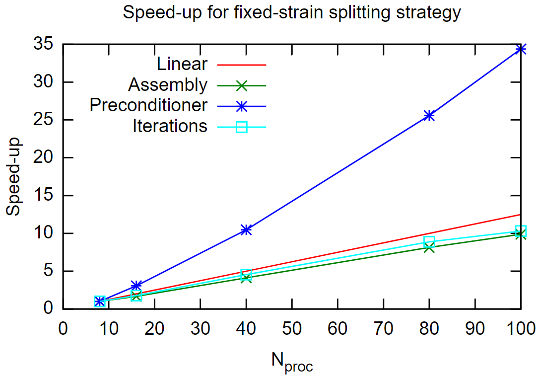
Measured computation times for monolithic and fixed-strain splitting methods are presented in tables 2 and 3. Total speed-up is presented at figure 4, while speed-ups for different computational stages for both strategies are presented in figure 5. Profiling results are presented in figure 6. Results show that fixed-strain strategy takes more time than monolithic one due to relatively large numbers (13 to 14) of splitting iterations at time steps. The fixed-strain strategy, however, scales better due to better scaling of iterations time, which is the most time-consuming part. Sublinear scaling of assembly procedure is explained by non-ideal partitioning by INMOST internal partitioner Inner_RCM, which is based on reverse Cuthill–McKee algorithm.


| , s | , s | , s | , s | #lin.it | |
|---|---|---|---|---|---|
| 8 | 2103 | 184 | 130 | 1761 | 1673 |
| 16 | 1592 | 148 | 101 | 1318 | 1637 |
| 40 | 457 | 40.3 | 16 | 379 | 2298 |
| 80 | 295 | 23.2 | 8.7 | 250 | 2522 |
| 100 | 235 | 17.9 | 5.8 | 206 | 2639 |
| , s | , s | , s | , s | #lin.it | |
|---|---|---|---|---|---|
| 8 | 7684 | 2479 | 219.5 | 4961 | 15162 |
| 16 | 4390 | 1483 | 71.5 | 2817 | 18121 |
| 40 | 1733 | 601.2 | 21.1 | 1091 | 19575 |
| 80 | 896 | 305.6 | 8.6 | 558.8 | 21099 |
| 100 | 749 | 251.7 | 6.4 | 480.8 | 21395 |



3.3 Problem B: real-life domain with synthetic elastic parameters
In this problem, a part of a real site is considered. The part is a quadrilateral cut in XY-plane from a domain with 9 geological layers and 11 different media. The media have are anisotropic with their hydraulic conductivity being a diagonal tensor with values ranging from to m/s. Specific storage coefficient varies from to m-1. Elastic parameters are not known and are set constant for all media: 10000 MPa, . One corner of the model has prescribed water head value m at 8th layer, which imitates injection in that layer. On the opposite side of the domain, constant water head value of m is set. Other boundaries are impermeable. Bottom boundary is fixed (), top boundary is free (), side boundaries have roller boundary conditions (zero normal displacement ). Simulation starts with constant initial water head value m and covers s ( 6.3 years).
Triangular prismatic mesh of 2205400 cells and 1142714 (total number of unknowns is 5461942) was constructed in the domain. Computations were performed on INM cluster using 40 – 600 cores. In order to obtain better balanced partitioning of the mesh, the ParMETIS parmetis partitioner was used, interface to which is provided by INMOST. Calculated water head and displacement distributions are depicted in figure 7. Time measurements and linear iterations count are presented in tables 4 and 5. Total speed-up is presented in figure 8 and shows superlinear scaling with monolithic strategy reaching slightly larger speed-up. In order to better understand this scaling behavior of the two strategies, speed-up for both assembly and linear solver are presented in figure 9 and profiling results are presented in figure 10. It can be seen that superlinear scaling is caused by linear solver, namely, scaling of the preconditioner. Such scaling is caused by the fact that drop tolerance, which is left at default value of , which makes MPTILUC preconditioner close enough to performing full LU decomposition of matrix diagonal sub-blocks. At the same time, assembly scales sublinearly, which is explained again by non-ideal partitioning of the mesh. Since profiling shows that assembly takes large percentage of time in the fixed-strain splitting, this strategy reaches lower overall speed-up.


| , s | , s | , s | , s | #lin.it | |
|---|---|---|---|---|---|
| 40 | 1490 | 52.0 | 688 | 731.5 | 470 |
| 120 | 490.5 | 19.5 | 58.0 | 406.7 | 680 |
| 200 | 247.5 | 11.5 | 51.1 | 180.5 | 742 |
| 280 | 157.8 | 9.4 | 16.2 | 129.5 | 779 |
| 360 | 141.0 | 7.0 | 24.6 | 107.1 | 902 |
| 440 | 100.6 | 6.1 | 10.1 | 82.4 | 821 |
| 520 | 84.7 | 5.2 | 6.3 | 71.6 | 840 |
| 600 | 81.9 | 4.7 | 5.7 | 69.9 | 993 |
| , s | , s | , s | , s | #lin.it | |
|---|---|---|---|---|---|
| 40 | 1101 | 81.3 | 475.3 | 537.4 | 728 |
| 120 | 340.3 | 31.0 | 28.9 | 278.1 | 1079 |
| 200 | 177.4 | 16.8 | 32.0 | 125.0 | 1101 |
| 280 | 114.9 | 14.8 | 8.6 | 90.5 | 1175 |
| 360 | 100.7 | 10.5 | 15.2 | 73.2 | 1290 |
| 440 | 85.8 | 8.9 | 5.5 | 69.5 | 1408 |
| 520 | 69.5 | 7.7 | 3.5 | 57.1 | 1399 |
| 600 | 64.0 | 7.1 | 3.3 | 52.4 | 1503 |


4 Conclusion
Two solution strategies for finite volume – virtual element discretizations of coupled poroelastic problems were tested in their parallel performance. Implemented using INMOST numerical platform, the model used a robust general-purpose linear solver. Calculations for two problems on meshes with millions of unknowns and up to 600 computational cores gave mixed results. Fixed-strain splitting strategy was expected to scale better due to performance of the linear solver, as separate systems for flow and mechanics have simpler structure. This, however, was not always observed. This is explained by the following reasons. First, performance of the linear solver is mostly determined by preconditioner, which exhibits superlinear scalability depending on the problem. Second, non-ideal performance of mesh partitioner results in sublinear scalability of systems assembly process, which affects splitting strategy more as assembly takes larger fraction of time in this case. Overall, there was no clear answer as to which strategy scales better. Partly this may imply that the linear solver used can successfully handle fully coupled multiphysical systems. However, with additional partitioner tuning to better balance mesh between processes, scalability of assembly may approach linear rate, resulting in better overall scalability of splitting strategy.
References
- (1) Birkholzer, J. T., Tsang, C. F., Bond, A. E., Hudson, J. A., Jing, L., Stephansson, O. (2019). 25 years of DECOVALEX-Scientific advances and lessons learned from an international research collaboration in coupled subsurface processes. International Journal of Rock Mechanics and Mining Sciences, 122, p. 103995.
- (2) Kapyrin, I. V., Ivanov, V. A., Kopytov, G. V., Utkin, S. S. (2015). Integral code GeRa for radioactive waste disposal safety validation. Gornyi Zh, (10), pp. 44-50.
- (3) GeRa website. gera.ibrae.ac.ru
- (4) Grigor’ev, F. V., Kapyrin, I. V., Vassilevski, Y. V. (2017). Modeling of thermal convection in porous media with volumetric heat source using the GeRa code. Chebyshevskii Sbornik, 18(3), pp. 235-254.
- (5) Kapyrin, I., Konshin, I., Kramarenko, V., Grigoriev, F. (2018, September). Modeling groundwater flow in unconfined conditions of variable density solutions in dual-porosity media using the GeRa code. In Russian Supercomputing Days (pp. 266-278). Springer, Cham.
- (6) Biot, M. A. (1941). General theory of three‐dimensional consolidation. Journal of applied physics, 12(2), pp. 155-164.
- (7) Keilegavlen, E., Nordbotten, J. M. (2017). Finite volume methods for elasticity with weak symmetry. International Journal for Numerical Methods in Engineering, 112(8), pp. 939-962.
- (8) Terekhov, K. M., Tchelepi, H. A. (2020). Cell-centered finite-volume method for elastic deformation of heterogeneous media with full-tensor properties. Journal of Computational and Applied Mathematics, 364, p. 112331.
- (9) Nordbotten, J. M., Keilegavlen, E. (2021). An introduction to multi-point flux (MPFA) and stress (MPSA) finite volume methods for thermo-poroelasticity. In Polyhedral Methods in Geosciences (pp. 119-158). Springer, Cham.
- (10) Terekhov, K. M. (2020). Cell-centered finite-volume method for heterogeneous anisotropic poromechanics problem. Journal of Computational and Applied Mathematics, 365, p. 112357.
- (11) Terekhov K. M., Vassilevski Y. V. (2022) Finite volume method for coupled subsurface flow problems, II: Poroelasticity. Journal of Computational Physics, 462, p. 111225.
- (12) Beirão da Veiga, L., Brezzi, F., Marini, L. D., Russo, A. (2014). The hitchhiker’s guide to the virtual element method. Mathematical models and methods in applied sciences, 24(08), 1541-1573.
- (13) Gain, A. L., Talischi, C., Paulino, G. H. (2014). On the virtual element method for three-dimensional linear elasticity problems on arbitrary polyhedral meshes. Computer Methods in Applied Mechanics and Engineering, 282, pp. 132-160.
- (14) Coulet, J., Faille, I., Girault, V., Guy, N., Nataf, F. (2020). A fully coupled scheme using virtual element method and finite volume for poroelasticity. Computational Geosciences, 24(2), pp. 381-403.
- (15) Aavatsmark, I., Barkve, T., Bøe, O., Mannseth, T. (1998). Discretization on unstructured grids for inhomogeneous, anisotropic media. Part I: Derivation of the methods. SIAM Journal on Scientific Computing, 19(5), pp. 1700-1716.
- (16) Kim, J., Tchelepi, H. A., Juanes, R. (2011). Stability and convergence of sequential methods for coupled flow and geomechanics: Fixed-stress and fixed-strain splits. Computer Methods in Applied Mechanics and Engineering, 200, pp. 1591-1606.
- (17) Frigo, M., Castelletto, N., Ferronato, M. (2022). Enhanced Relaxed Physical Factorization preconditioner for coupled poromechanics. Computers & Mathematics with Applications, 106, pp. 27-39.
- (18) INMOST website. inmost.org
- (19) Vassilevski, Y., Terekhov, K., Nikitin, K., Kapyrin, I. (2020). Parallel finite volume computation on general meshes. New York: Springer International Publishing.
- (20) Anuprienko, D., Kapyrin, I. (2021). Nonlinearity continuation method for steady-state groundwater flow modeling in variably saturated conditions. Journal of Computational and Applied Mathematics, 393, p. 113502.
- (21) Kolditz, O., Shao, H., Wang, W., Bauer, S. (2016). Thermo-hydro-mechanical chemical processes in fractured porous media: modelling and benchmarking (Vol. 25). Berlin: Springer.
- (22) INM RAS cluster. cluster2.inm.ras.ru
- (23) Karypis, G., Schloegel, K., & Kumar, V. (1997). Parmetis: Parallel graph partitioning and sparse matrix ordering library.