跳到论文正文
W Papers独立论文阅读器 arXiv:2210.06202 论文正文 计算阅读时间 · 0%
引用这篇论文根据当前论文元数据生成,正式投稿前建议核对。


License: arXiv.org perpetual non-exclusive license
arXiv:2210.06202v1 [math.NA] 09 Aug 2022

A general theoretical scheme for shape-programming of incompressible hyperelastic shells through differential growth

Zhanfeng Li Affiliation: School of Civil Engineering and Transportation, South China University of Technology, Guangzhou, China Affiliation: Zienkiewicz Centre for Computational Engineering (ZCCE), Swansea University, Swansea, United Kingdom    Jiong Wang Thanks: Corresponding author. Email: ctjwang@scut.edu.cn Tel.: +86 13926459861, Fax: +86 21-87114460. Affiliation: School of Civil Engineering and Transportation, South China University of Technology, Guangzhou, China Affiliation: State Key Laboratory of Subtropical Building Science, South China University of Technology, Guangzhou, China    Mokarram Hossain Affiliation: Zienkiewicz Centre for Computational Engineering (ZCCE), Swansea University, Swansea, United Kingdom    Chennakesava Kadapa Affiliation: School of Engineering and the Built Environment, Edinburgh Napier University, Edinburgh, United Kingdom
Abstract

In this paper, we study the problem of shape-programming of incompressible hyperelastic shells through differential growth. The aim of the current work is to determine the growth tensor (or growth functions) that can produce the deformation of a shell to the desired shape. First, a consistent finite-strain shell theory is introduced. The shell equation system is established from the 3D governing system through a series expansion and truncation approach. Based on the shell theory, the problem of shape-programming is studied under the stress-free assumption. For a special case in which the parametric coordinate curves generate a net of curvature lines on the target surface, the sufficient condition to ensure the vanishing of the stress components is analyzed, from which the explicit expression of the growth tensor can be derived. In the general case, we conduct the variable changes and derive the total growth tensor by considering a two-step deformation of the shell. With these obtained results, a general theoretical scheme for shape-programming of thin hyperelastic shells through differential growth is proposed. To demonstrate the feasibility and efficiency of the proposed scheme, several nature-inspired examples are studied. The derived growth tensors in these examples have also been implemented in the numerical simulations to verify their correctness and accuracy. The simulation results show that the target shapes of the shell samples can be recovered completely. The scheme for shape-programming proposed in the current work is helpful in designing and manufacturing intelligent soft devices.

Keywords Hyperelastic shell ⋅\cdot Differential growth ⋅\cdot Shape-programming ⋅\cdot Theoretical scheme ⋅\cdot Numerical simulations

1 Introduction

Growth of soft biological tissues and swelling (or expansion) of soft polymeric gels are commonly observed in nature (Ambrosi et al. 2011; Liu et al. 2015). Due to the inhomogeneity or incompatibility of the growth fields, soft material samples usually exhibit diverse morphological changes and surface pattern evolutions during the growing processes, which is referred to as the ‘differential growth’ and has attracted extensive research interest in recent years (Goriely and Ben Amar 2005; Li et al. 2012; Kempaiah and Nie 2014; Huang et al. 2018). To fulfill the requirements of engineering applications, it is usually desired that the configurations of soft material samples are controllable during the growing processes, such that certain kinds of functions are realized. This goal can be achieved through sophisticated composition or architectural design in the soft material samples. The technique is known as ‘shape-programming’ (Liu et al. 2016; van Manen et al. 2018), which has been utilized for manufacturing a variety of intelligent soft devices, e.g., biomimetic 4D printing of flowers (Gladman et al. 2016), pressure-actuated deforming plate (Siéfert et al. 2019), pasta with transient morphing effect (Tao et al. 2021), and polymorphic metal-elastomer composite (Hwang et al. 2022).

From the viewpoint of solid mechanics, soft materials can be treated as certain kinds of hyperelastic materials. The growth field in a soft material sample is usually modeled by incorporating a growth tensor. Due to the residual stresses triggered by the incompatibility of the growth field, as well as the external loads and boundary restrictions, the sample also undergoes elastic deformations. Thus, the total deformation gradient tensor should be decomposed into an elastic strain tensor and a growth tensor (Kondaurov and Nikitin 1987; Rodriguez et al. 1994; Ben Amar and Goriely 2005). The elastic incompressible constraint should also be adopted since the elastic deformations of soft materials are typically isochoric (Wex et al. 2015; Kadapa et al. 2021). Based on these constitutive and kinematic assumptions, the growth behaviors of soft material samples can be studied by solving the system of mechanical field equations. Because of the inherent nonlinearities in the large growth-induced deformations, mechanical instabilities can also be triggered in the soft material samples (Ben Amar and Goriely 2005; Li et al. 2011; Goriely 2017; Pezzulla et al. 2018; Xu et al. 2020).

Despite the numerous studies on the growth behaviors of soft material samples, the majority of the modeling works pay attention to the direct problem, i.e., determining the deformations of soft material samples when the growth fields are specified. However, in order to utilize the shape-programming technique for engineering applications, one needs to study the inverse problem. That is, how to determine the growth fields in the samples such that the current configurations induced by differential growth can achieve any target shapes? This inverse problem has also been studied in some previous works (Dias et al. 2011; Jones and Mahadevan 2015; Acharya 2019; Wang et al. 2019a; Nojoomi et al. 2021; Li et al. 2022; Wang et al. 2022, cf.). In these works, the initial configurations of soft material samples usually have the thin plate form. Although the shell form is more common in nature and engineering fields, it is seldom chosen as the initial configuration of the soft material samples due to the difficulties associated with modelling shell structures.

To achieve the goal of shape-programming, a prerequisite is to predict the relations between the growth fields and the morphologies of soft material samples. It is thus of significance to establish an efficient and accurate mathematical model by taking configurations of samples, material properties, boundary conditions and other factors into account. In terms of shell theories for growth deformations, the Kirchhoff shell theory has been adopted to describe mechanical behavior in growing soft membranes (Vetter et al. 2013; Rausch and Kuhl 2014), which relies on ad hoc assumptions of the stress components and deformation gradient. Another shell theory is proposed based on the non-Euclidean geometry, where the deformation of samples is determined by the intrinsic geometric properties attached to surfaces, such as the first and second fundamental forms, and the applied growth fields (Souhayl Sadik et al. 2016; Pezzulla et al. 2018). In Song and Dai 2016, a consistent finite-strain shell theory has been proposed within the framework of nonlinear elasticity, where the shell equation is derived from the 3D formulation through a series-expansion and truncation approach. To apply this theory for growth-induced deformations, Yu et al. 2022 incorporated the growth effect through the decomposition of the deformation gradient and derived the shell equation system for soft shell samples.

In this paper, we aim to propose a general theoretical scheme for shape-programming of incompressible hyperelastic shells through differential growth. Following the shell theory proposed in Yu et al. 2022, the shell equation system is established from the 3D governing system, where a series expansion and truncation approach is adopted. To fulfill the purpose of shape-programming, the shell equation system is tackled by assuming that all the stress components vanish. Under this stress-free assumption, we first consider a special case in which the parametric coordinate curves generate a net of curvature lines on the target surface. By analyzing the sufficient condition to ensure the vanishing of the stress components, the explicit expression of the growth tensor is derived (i.e., the inverse problem is solved), which depends on the intrinsic geometric properties of the target surface. In the general case that the parametric coordinate curves cannot generate a net of curvature lines on the target surface, we conduct the variable changes and derive the total growth tensor by considering a two-step deformation of the shell sample. Based on these results, a theoretical scheme for shape-programming of hyperelastic shells is formulated. The feasibility and efficiency of this scheme are demonstrated by studying several typical examples.

This paper is organized as follows. In section 2, the finite-strain shell theory for modeling the growth behaviors of thin hyperelastic shells is introduced. In section 3, the problem of shape programming is solved and the theoretical scheme is proposed. In section 4, some typical examples are studied to show the efficiency of the theoretical scheme. Finally, some conclusions are drawn. In the following notations, the Greek letters (α,β,γ​…)(\alpha,\beta,\gamma...) run from 1 to 2, and the Latin letters (i,j,k​…)(i,j,k...) run from 1 to 3. The repeated summation convention is employed and a comma preceding indices (⋅),{(\cdot)}_{,} represents the differentiation.

2 The finite-strain shell theory

In this section, we first formulate the 3D governing system for modeling the growth behavior of a thin hyperelastic shell. Then, through a series-expansion and truncation approach, the finite-strain shell equation system of growth will be established.

2.1 Kinematics and the 3D governing system

We consider a thin homogeneous hyperelastic shell locating in the three-dimensional (3D) Euclidean space R3R^{3}. Within an orthonormal frame {O;𝐞1,𝐞2,𝐞3}\{O;\mathbf{e}_{1},\mathbf{e}_{2},\mathbf{e}_{3}\}, the reference configuration of the shell occupies the region 𝒦r=𝒮r×[0,2​h]\mathcal{K}_{r}=\mathcal{S}_{r}\times[0,2h], where the thickness parameter hh is much smaller than the dimensions of the base (bottom) surface 𝒮r\mathcal{S}_{r} and its local radius of curvature. The position vector of a material point in the reference configuration 𝒦r\mathcal{K}_{r} is denoted by 𝐗=Xi​𝐞i\mathbf{X}=X^{i}\mathbf{e}_{i} (cf. Fig. 1(a)). The geometric description of a shell has been systematically reported in the literature (Ciarlet 2005; Steigmann 2012; Song and Dai 2016, cf.), which is simply introduced below.

First, a curvilinear coordinate system {θα}α=1,2\{\theta^{\alpha}\}_{\alpha=1,2} is utilized to parametrize the base surface 𝒮r\mathcal{S}_{r} of the shell in the reference configuration, which yields the parametric equation as

𝐬⁡(θα)={X1​(θα),X2​(θα),X3​(θα)},(θα)α=1,2∈Ωr.\mathbf{s}(\theta^{\alpha})=\left\{X^{1}(\theta^{\alpha}),X^{2}(\theta^{\alpha}),X^{3}(\theta^{\alpha})\right\},\quad(\theta^{\alpha})_{\alpha=1,2}\in\Omega_{r}. (1)

This parametric equation represents a continuous map from the region Ωr⊂R2\Omega_{r}\subset R^{2} to the surface 𝒮r⊂R3\mathcal{S}_{r}\subset R^{3}. At a generic point on 𝒮r\mathcal{S}_{r}, the tangent vectors along the coordinate curves are given by 𝐠α=𝐬,α=∂𝐬/∂θα\mathbf{g}_{\alpha}=\mathbf{s}_{,\alpha}=\partial\mathbf{s}/\partial\theta^{\alpha}, which span the tangent plane to the surface 𝒮r\mathcal{S}_{r} at that point. The two vectors {𝐠α}α=1,2\{\mathbf{g}_{\alpha}\}_{\alpha=1,2} are also referred to as the covariant basis of the tangent plane. Another two vectors {𝐠α}α=1,2\{\mathbf{g}^{\alpha}\}_{\alpha=1,2} on the tangent plane can be determined unambiguously through the relations 𝐠α⋅𝐠β=δαβ\mathbf{g}_{\alpha}\cdot\mathbf{g}^{\beta}=\delta_{\alpha}^{\beta}, which form the contravariant basis of the tangent plane. Then, the unit normal vector of the surface 𝒮r\mathcal{S}_{r} should be defined by 𝐧=(𝐠1∧𝐠2)/|𝐠1∧𝐠2|\mathbf{n}=(\mathbf{g}_{1}\wedge\mathbf{g}_{2})/\left|\mathbf{g}_{1}\wedge\mathbf{g}_{2}\right| (cf. Fig. 1(b)). By denoting 𝐠3=𝐠3=𝐧\mathbf{g}_{3}=\mathbf{g}^{3}=\mathbf{n}, {𝐠i}i=1,2,3\{\mathbf{g}_{i}\}_{i=1,2,3} and {𝐠i}i=1,2,3\{\mathbf{g}^{i}\}_{i=1,2,3} constitute two sets of right-handed orthogonal bases on the base surface 𝒮r\mathcal{S}_{r}. The first and second fundamental forms of the surface 𝒮r\mathcal{S}_{r} can be written into

Ir=gα​β​d​θα​d​θβ,IIr=bα​β​d​θα​d​θβ,\mathrm{I}_{r}=g_{\alpha\beta}d\theta^{\alpha}d\theta^{\beta},\ \ \ \mathrm{II}_{r}=b_{\alpha\beta}d\theta^{\alpha}d\theta^{\beta}, (2)

where gα​β=𝐠α⋅𝐠βg_{\alpha\beta}=\mathbf{g}_{\alpha}\cdot\mathbf{g}_{\beta} and bα​β=𝐬,αβ⋅𝐧b_{\alpha\beta}=\mathbf{s}_{,\alpha\beta}\cdot\mathbf{n} are the fundamental quantities. Conventionally, the fundamental quantities are also denoted by

Er=g11,Fr=g12=g21,Gr=g22,\displaystyle E_{r}=g_{11},\quad F_{r}=g_{12}=g_{21},\quad G_{r}=g_{22}, (3)
Lr=b11,Mr=b12=b21,Nr=b22.\displaystyle L_{r}=b_{11},\quad M_{r}=b_{12}=b_{21},\quad N_{r}=b_{22}.
Refer to caption
Figure 1: Position vector in the reference configuration 𝒦r\mathcal{K}_{r}: (a) reference configuration of the shell and decomposition of the position vector 𝐗\mathbf{X}; (b) the curvilinear coordinate system and the local covariant basis on the base surface 𝒮r\mathcal{S}_{r} of the shell.

As shown in Fig.1(a), the position vector 𝐗\mathbf{X} of a material point in the reference configuration 𝒦r\mathcal{K}_{r} of the shell can be decomposed into

𝐗=𝐬⁡(θα)+Z​𝐧​(θα),0≤Z≤2​h,\mathbf{X}=\mathbf{s}(\theta^{\alpha})+Z\mathbf{n}(\theta^{\alpha}),\quad 0\leq Z\leq 2h, (4)

where ZZ is the coordinate of the point along the normal direction 𝐧\mathbf{n}. Accordingly, the differential of 𝐗\mathbf{X} yields that

d𝐗=d𝐬+Zd𝐧+𝐧dZ=𝐠αdθα+Z𝐧,αdθα+𝐧dZ.d\mathbf{X}=d\mathbf{s}+Zd\mathbf{n}+\mathbf{n}dZ=\mathbf{g}_{\alpha}d\theta^{\alpha}+Z\mathbf{n}_{,\alpha}d\theta^{\alpha}+\mathbf{n}dZ. (5)

From the Weingarten equation(Chen 2017), we have

d𝐧=𝐧,αdθα=(𝐧,α⊗𝐠α)𝐠βdθβ=−𝕂d𝐬,d\mathbf{n}=\mathbf{n}_{,\alpha}d\theta^{\alpha}=\left(\mathbf{n}_{,\alpha}\otimes\mathbf{g}^{\alpha}\right)\mathbf{g}_{\beta}d\theta^{\beta}=-\mathbb{K}d\mathbf{s}, (6)

where 𝕂=−𝐧,α⊗𝐠α\mathbb{K}=-\mathbf{n}_{,\alpha}\otimes\mathbf{g}^{\alpha} is the curvature tensor. The mean and Gaussian curvatures of the surface 𝒮r\mathcal{S}_{r} are given by

H=12​tr​(𝕂),K=Det⁡(𝕂).H=\frac{1}{2}\mathrm{tr}\left(\mathbb{K}\right),\quad K=\mathrm{Det}\left(\mathbb{K}\right). (7)

By substituting (6) into (5), we obtain

d​𝐗=𝕌​d​𝐬+𝐧​d​Z=𝐠^α​d​θα+𝐧​d​Z,d\mathbf{X}=\mathbb{U}d\mathbf{s}+\mathbf{n}dZ=\hat{\mathbf{g}}_{\alpha}d\theta^{\alpha}+\mathbf{n}dZ, (8)

where 𝕌=𝐠α⊗𝐠α−Z​𝕂\mathbb{U}=\mathbf{g}_{\alpha}\otimes\mathbf{g}^{\alpha}-Z\mathbb{K} and 𝐠^α=𝕌​𝐠α\hat{\mathbf{g}}_{\alpha}=\mathbb{U}\mathbf{g}_{\alpha}. We further denote 𝐠^α=𝕌−T​𝐠α\hat{\mathbf{g}}^{\alpha}=\mathbb{U}^{-T}\mathbf{g}^{\alpha}, then {𝐠^α}α=1,2\{\hat{\mathbf{g}}_{\alpha}\}_{\alpha=1,2} and {𝐠^α}α=1,2\{\hat{\mathbf{g}}^{\alpha}\}_{\alpha=1,2} form the covariant and contravariant base vectors at an arbitrary point in the shell, which are also orthogonal to 𝐧\mathbf{n}. Notice that the thickness of the shell is much smaller than the radius of curvature of 𝒮r\mathcal{S}_{r}; thus, 𝕌\mathbb{U} should be an invertible tensor. From (8), the area element on the base surface and the volume element in the shell can be written into

d​A=|𝐠1∧𝐠2|​d​θ1​d​θ2=g11​g22−g122​d​θ1​d​θ2,\displaystyle dA=\left|\mathbf{g}_{1}\wedge\mathbf{g}_{2}\right|d\theta^{1}d\theta^{2}=\sqrt{g_{11}g_{22}-g_{12}^{2}}\ d\theta^{1}d\theta^{2}, (9)
d​V=Det⁡(𝕌)​d​A​d​Z=(1−2​H​Z+K​Z2)​d​A​d​Z.\displaystyle dV=\mathrm{Det}(\mathbb{U})dAdZ=\left(1-2HZ+KZ^{2}\right)dAdZ.

Regarding area element on the lateral surface d​ada, the local differential follows (8) that

𝐍​d​a=(𝕌​𝝉)×𝐧​d​s​d​Z,\mathbf{N}da=(\mathbb{U}\bm{\tau})\times\mathbf{n}\ dsdZ, (10)

where 𝐍\mathbf{N} is the outward normal unit vector of the lateral surface, and 𝝉\bm{\tau} is the unit tangent vector along the edge curve ∂𝒮r\partial\mathcal{S}_{r} of the base surface, and ss is the arc-length variable on the edge curve ∂𝒮r\partial\mathcal{S}_{r} of the base surface. The norm of vector (𝕌​𝝉)×𝐧(\mathbb{U}\bm{\tau})\times\mathbf{n} is denoted by gτ\sqrt{g_{\tau}} such that d​a=gτ​d​s​d​Zda=\sqrt{g_{\tau}}dsdZ.

Due to the growth effect and the external loads, the configuration of the shell will deform from 𝒦r\mathcal{K}_{r} to the current configuration 𝒦t\mathcal{K}_{t} in ℛ3\mathcal{R}^{3}. Within the orthonormal frame {O;𝐞1,𝐞2,𝐞3}\{O;\mathbf{e}_{1},\mathbf{e}_{2},\mathbf{e}_{3}\}, the position vector of a material point in 𝒦t\mathcal{K}_{t} is denoted by 𝐱⁡(θα,Z)=xi​(θα,Z)​𝐞i\mathbf{x}(\theta^{\alpha},Z)=x^{i}(\theta^{\alpha},Z)\mathbf{e}_{i}. The deformation gradient tensor 𝔽\mathbb{F} can then be calculated through

𝔽=𝐱,α⊗𝐠^α+∂𝐱∂Z⊗𝐧=(∇𝐱)𝕌−1+∂𝐱∂Z⊗𝐧,\displaystyle\mathbb{F}=\mathbf{x}_{,\alpha}\otimes\hat{\mathbf{g}}^{\alpha}+\frac{\partial\mathbf{x}}{\partial Z}\otimes\mathbf{n}=\left(\nabla\mathbf{x}\right)\mathbb{U}^{-1}+\frac{\partial\mathbf{x}}{\partial Z}\otimes\mathbf{n}, (11)

where ∇\nabla is the in-plane 2-D gradient on the base surface 𝒮r\mathcal{S}_{r} (∇𝐱=𝐱,α⊗𝐠α\nabla\mathbf{x}=\mathbf{x}_{,\alpha}\otimes\mathbf{g}^{\alpha}).

Following the basic assumption of growth mechanics (Kondaurov and Nikitin 1987; Rodriguez et al. 1994; Ben Amar and Goriely 2005; Groh 2022; Dortdivanlioglu et al. 2017; Mehta et al. 2021), the deformation gradient tensor 𝔽\mathbb{F} is decomposed into

𝔽=𝔸​𝔾,\mathbb{F}=\mathbb{A}\mathbb{G}, (12)

where 𝔸\mathbb{A} is the elastic strain tensor and 𝔾\mathbb{G} is the growth tensor. It is known that the rate of growth is relatively slow compared with the elastic response of the material, thus the distribution of the growth tensor 𝔾\mathbb{G} in the shell is assumed to be given and does not change.

As the elastic deformations of soft materials (e.g., soft biological tissues, polymeric gels) are generally isochoric, the following constraint equation should be adopted

R⁡(𝔽,𝔾)=JG​R0​(𝔸)=JG​(Det⁡(𝔸)−1)=0,R(\mathbb{F},\mathbb{G})=J_{G}R_{0}(\mathbb{A})=J_{G}\left(\operatorname{Det}(\mathbb{A})-1\right)=0, (13)

where JG=Det⁡(𝔾)J_{G}=\operatorname{Det}(\mathbb{G}). Furthermore, we suppose the material has an elastic strain-energy function

ϕ⁡(𝔽,𝔾)=JG​ϕ0​(𝔸)=JG​ϕ0​(𝔽​𝔾−1).\phi(\mathbb{F},\mathbb{G})=J_{G}\phi_{0}(\mathbb{A})=J_{G}\phi_{0}(\mathbb{FG}^{-1}). (14)

Then, the nominal stress tensor 𝕊\mathbb{S} can be calculated through the constitutive equation

𝕊=∂ϕ∂𝔽−p​∂R∂𝔽=JG​𝔾−1​(∂ϕ0​(𝔸)∂𝔸−p​∂R0​(𝔸)∂𝔸),\mathbb{S}=\frac{\partial\phi}{\partial\mathbb{F}}-p\frac{\partial R}{\partial\mathbb{F}}=J_{G}\mathbb{G}^{-1}\left(\frac{\partial\phi_{0}(\mathbb{A})}{\partial\mathbb{A}}-p\frac{\partial R_{0}(\mathbb{A})}{\partial\mathbb{A}}\right), (15)

where p⁡(θα,Z)p(\theta^{\alpha},Z) is the Lagrange multiplier associated with the constraint (13).

During the growing process, the hyperelastic shell satisfies the following mechanical equilibrium equation

Div⁡𝕊\displaystyle\operatorname{Div}\mathbb{S} =(𝕊,α)T𝐠^α+(∂𝕊∂Z)T𝐧=𝟎,in𝒮r×[0,2h].\displaystyle=\left(\mathbb{S}_{,\alpha}\right)^{T}\hat{\mathbf{g}}^{\alpha}+\left(\frac{\partial\mathbb{S}}{\partial Z}\right)^{T}\mathbf{n}=\mathbf{0},\quad\text{in}\ \ \mathcal{S}_{r}\times[0,2h]. (16)

We suppose that the bottom and top surfaces of the shell are subjected to the applied traction 𝐪±\mathbf{q}^{\pm}, which yields the boundary conditions

𝕊T𝐧|Z=0=−𝐪−,𝕊T𝐧|Z=2​h=𝐪+,on𝒮r.\mathbb{S}^{T}\mathbf{n}|_{Z=0}=-\mathbf{q}^{-},\quad\mathbb{S}^{T}\mathbf{n}|_{Z=2h}=\mathbf{q}^{+},\ \ \mathrm{on}\ \ \mathcal{S}_{r}. (17)

On the lateral surface ∂𝒮r×[0,2​h]\partial\mathcal{S}_{r}\times[0,2h] of the shell, we suppose the applied traction is 𝐪⁡(s,Z)\mathbf{q}(s,Z), where ss is the arc-length variable of boundary curve ∂𝒮r\partial\mathcal{S}_{r}. So, we also have the boundary condition

𝕊T​𝐍=𝐪⁡(s,Z)on∂𝒮r×[0,2​h].\mathbb{S}^{T}\mathbf{N}=\mathbf{q}(s,Z)\quad\mathrm{on}\quad\partial\mathcal{S}_{r}\times[0,2h]. (18)

Eqs. (13) and (16) together with the boundary conditions (17) and (18) constitute the 3D governing system of the shell model, which contains the unknowns {𝐱,p}\{\mathbf{x},p\}.

2.2 Shell equation system

Starting from the 3D governing system of the shell model, the shell equation system can be derived through a series-expansion and a truncation approach. This approach has been proposed in Dai and Song 2014; Song and Dai 2016; Wang et al. 2016 for developing the consistent finite-strain plate and shell theories without the growth effect. In Wang et al. 2018; Yu et al. 2022, the finite-strain plate and shell theories of growth have also been established through this approach. For the sake of completeness of the current paper, the key steps of this approach to derive the shell equation system are introduced below (see Yu et al. 2022 for a comprehensive introduction). It should be noted that the derived shell equation system can attain the accuracy of O⁡(h2)O(h^{2}). However, to fulfill the requirements of shape-programming in the following sections, we only need to present the shell equation to the asymptotic order of O⁡(h)O(h).

To eliminate the thickness variable ZZ from the 3D governing system, we first conduct the series expansions of the unknowns as follows

𝐱(θα,Z)=∑n=02𝐱(n)n!Zn+O(Z3),p(θα,Z)=∑n=02p(n)n!Zn+O(Z3),\displaystyle\mathbf{x}(\theta^{\alpha},Z)=\sum_{n=0}^{2}\frac{\mathbf{x}^{(n)}}{n!}Z^{n}+O\left(Z^{3}\right),\quad p(\theta^{\alpha},Z)=\sum_{n=0}^{2}\frac{p^{(n)}}{n!}Z^{n}+O\left(Z^{3}\right), (19)

where (⋅)(n)=∂n(⋅)/∂Zn|Z=0(\cdot)^{(n)}=\partial^{n}(\cdot)/\left.\partial Z^{n}\right|_{Z=0}. According to (19), the deformation gradient tensor 𝔽\mathbb{F}, the elastic strain tensor 𝔸\mathbb{A} and the nominal stress tensor 𝕊\mathbb{S} can also be expanded as

𝔽\displaystyle\mathbb{F} =𝔽(0)+Z​𝔽(1)+O⁡(Z2),\displaystyle=\mathbb{F}^{(0)}+Z\mathbb{F}^{(1)}+O(Z^{2}), (20)
𝔸\displaystyle\mathbb{A} =𝔸(0)+Z​𝔸(1)+O⁡(Z2),\displaystyle=\mathbb{A}^{(0)}+Z\mathbb{A}^{(1)}+O(Z^{2}),
𝕊\displaystyle\mathbb{S} =𝕊(0)+Z​𝕊(1)+O⁡(Z2).\displaystyle=\mathbb{S}^{(0)}+Z\mathbb{S}^{(1)}+O(Z^{2}).

Furthermore, we denote

𝔾=𝔾(0)+Z​𝔾(1)+O⁡(Z2),\displaystyle\mathbb{G}=\mathbb{G}^{(0)}+Z\mathbb{G}^{(1)}+O(Z^{2}), (21)
𝔾−1=𝔾¯(0)+Z​𝔾¯(1)+O⁡(Z2),\displaystyle\mathbb{G}^{-1}=\bar{\mathbb{G}}^{(0)}+Z\bar{\mathbb{G}}^{(1)}+O(Z^{2}),
JG​𝔾−1=𝔾^(0)+Z​𝔾^(1)+O⁡(Z2).\displaystyle J_{G}\mathbb{G}^{-1}=\hat{\mathbb{G}}^{(0)}+Z\hat{\mathbb{G}}^{(1)}+O(Z^{2}).

Once the growth tensor 𝔾\mathbb{G} is given, 𝔾¯(n)\bar{\mathbb{G}}^{(n)} and 𝔾^(n)\hat{\mathbb{G}}^{(n)} (n=0,1)(n=0,1) can be calculated directly.

By using the kinematic relations (11) and (12), the concrete expressions of 𝔽(n)\mathbb{F}^{(n)} and 𝔸(n)\mathbb{A}^{(n)} (n=0,1)(n=0,1) in terms of 𝐱(n)\mathbf{x}^{(n)} (n=0,1,2)(n=0,1,2) can be derived. Further from the constitutive equation (15), we obtain

𝕊(0)\displaystyle\mathbb{S}^{(0)} =𝔾^(0)​(𝒜(0)−p(0)​ℛ(0)),\displaystyle=\hat{\mathbb{G}}^{(0)}\left(\mathcal{A}^{(0)}-p^{(0)}\mathcal{R}^{(0)}\right), (22)
𝕊(1)\displaystyle\mathbb{S}^{(1)} =𝔾^(0)(𝒜(1):𝔸(1)−p(0)ℛ(1):𝔸(1)−p(1)ℛ(0))+𝔾^(1)(𝒜(0)−p(0)ℛ(0)),\displaystyle=\hat{\mathbb{G}}^{(0)}\left(\mathcal{A}^{(1)}:\mathbb{A}^{(1)}-p^{(0)}\mathcal{R}^{(1)}:\mathbb{A}^{(1)}-p^{(1)}\mathcal{R}^{(0)}\right)+\hat{\mathbb{G}}^{(1)}\left(\mathcal{A}^{(0)}-p^{(0)}\mathcal{R}^{(0)}\right),

where 𝒜(n)=∂n+1ϕ0/∂𝔸n+1|𝔸=𝔸(0)\mathcal{A}^{(n)}=\partial^{n+1}\phi_{0}/\partial\mathbb{A}^{n+1}|_{\mathbb{A}=\mathbb{A}^{(0)}} and ℛ(n)=∂n+1R0/∂𝔸n+1|𝔸=𝔸(0)\mathcal{R}^{(n)}=\partial^{n+1}R_{0}/\partial\mathbb{A}^{n+1}|_{\mathbb{A}=\mathbb{A}^{(0)}} (n=0,1)(n=0,1).

We substitute (19) and (20) into the constraint equation (13) and the mechanical equilibrium equation (16). The coefficients of ZnZ^{n} (n=0,1)(n=0,1) in these equations should be zero, which yield that

Det(𝔸(0))−1=0,ℛ(0):𝔸(1)=0,\displaystyle\mathrm{Det}\left(\mathbb{A}^{(0)}\right)-1=0,\quad\mathcal{R}^{(0)}:\mathbb{A}^{(1)}=0, (23)

and

∇⋅𝕊(0)+(𝕊(1))T​𝐧=𝟎,\displaystyle\nabla\cdot\mathbb{S}^{(0)}+\left(\mathbb{S}^{(1)}\right)^{T}\mathbf{n}=\mathbf{0}, (24)
∇⋅𝕊(1)+(𝕊(2))T𝐧+𝕂T𝐠α⋅𝕊(0),α=𝟎.\displaystyle\nabla\cdot\mathbb{S}^{(1)}+\left(\mathbb{S}^{(2)}\right)^{T}\mathbf{n}+\mathbb{K}^{T}\mathbf{g}^{\alpha}\cdot\mathbb{S}^{(0)}_{,\alpha}=\mathbf{0}.

Further substituting (19) and (20) into the boundary conditions (17), another two equations can be obtained

(𝕊(0))T​𝐧=−𝐪−,\displaystyle\left(\mathbb{S}^{(0)}\right)^{T}\mathbf{n}=-\mathbf{q}^{-}, (25)
(𝕊(0)+2​h​𝕊(1)+2​h2​𝕊(2))T​𝐧=𝐪+.\displaystyle\left(\mathbb{S}^{(0)}+2h\mathbb{S}^{(1)}+2h^{2}\mathbb{S}^{(2)}\right)^{T}\mathbf{n}=\mathbf{q}^{+}.

Eqs. (23)2 and (24)1 constitute a linear system for 𝐱(2)\mathbf{x}^{(2)} and p(1)p^{(1)}. By solving these two equations, we obtain (Yu et al. 2022)

𝐱(2)=𝔻−1​(p(1)​𝐲−𝐟),p(1)=𝐲⋅𝔻−1​𝐟−T𝐲⋅𝔻−1​𝐲,\mathbf{x}^{(2)}=\mathbb{D}^{-1}\left(p^{(1)}\mathbf{y}-\mathbf{f}\right),\ \quad p^{(1)}=\frac{\mathbf{y}\cdot\mathbb{D}^{-1}\mathbf{f}-T}{\mathbf{y}\cdot\mathbb{D}^{-1}\mathbf{y}}, (26)

where

(𝔻)i​j=\displaystyle(\mathbb{D})_{ij}= Det⁡(𝔾(0))​(𝒜(1)−p(0)​ℛ(1))k​i​l​j​((𝔾¯(0))T​𝐧)k​((𝔾¯(0))T​𝐧)l,\displaystyle\mathrm{Det}(\mathbb{G}^{(0)})\left(\mathcal{A}^{(1)}-p^{(0)}\mathcal{R}^{(1)}\right)_{kilj}\left(\left(\bar{\mathbb{G}}^{(0)}\right)^{T}\mathbf{n}\right)_{k}\left(\left(\bar{\mathbb{G}}^{(0)}\right)^{T}\mathbf{n}\right)_{l},
𝐲=\displaystyle\mathbf{y}= ℛ(0)T​𝔾^(0)T​𝐧,\displaystyle\mathcal{R}^{(0)^{T}}\hat{\mathbb{G}}^{(0)^{T}}\mathbf{n},
𝐟=\displaystyle\mathbf{f}= [(𝒜(1)−p(0)ℛ(1)):[𝔽(0)𝔾¯(1)+(𝐱(1)⊗∇+𝐱(0)⊗𝕂)𝔾¯(0)]]T𝔾^(0)T𝐧\displaystyle\Big[\left(\mathcal{A}^{(1)}-p^{(0)}\mathcal{R}^{(1)}\right):\left[\mathbb{F}^{(0)}\bar{\mathbb{G}}^{(1)}+\left(\mathbf{x}^{(1)}\otimes\nabla+\mathbf{x}^{(0)}\otimes\mathbb{K}\right)\bar{\mathbb{G}}^{(0)}\right]\Big]^{T}\hat{\mathbb{G}}^{(0)^{T}}\mathbf{n}
+(𝒜(0)−p(0)​ℛ(0))T​𝔾^(1)T​𝐧+∇⋅𝕊(0),\displaystyle+\left(\mathcal{A}^{(0)}-p^{(0)}\mathcal{R}^{(0)}\right)^{T}\hat{\mathbb{G}}^{(1)^{T}}\mathbf{n}+\nabla\cdot\mathbb{S}^{(0)},
T=\displaystyle T= Det(𝔾(0))ℛ(0):[(𝐱(1)⊗∇+𝐱(0)⊗∇𝕂)𝔾¯(0)+𝔽(0)𝔾¯(1)].\displaystyle\mathrm{Det}(\mathbb{G}^{(0)})\mathcal{R}^{(0)}:\left[\left(\mathbf{x}^{(1)}\otimes\nabla+\mathbf{x}^{(0)}\otimes\nabla\mathbb{K}\right)\bar{\mathbb{G}}^{(0)}+\mathbb{F}^{(0)}\bar{\mathbb{G}}^{(1)}\right].

The expressions of 𝐱(1)\mathbf{x}^{(1)} and p(0)p^{(0)} in terms of 𝐱(0)\mathbf{x}^{(0)} can be obtained by solving the equations (23)1 and (25)1. However, as these two equations are non-linear, the explicit expressions of 𝐱(1)\mathbf{x}^{(1)} and p(0)p^{(0)} can only be presented when a concrete form of the strain-energy function ϕ0​(𝔸)\phi_{0}(\mathbb{A}) is given.

To incorporate the effect of curvature of the shell, the factor Det⁡(𝕌)|Z=2​h=1−4​h​H+4​h2​K\mathrm{Det}(\mathbb{U})|_{Z=2h}=1-4hH+4h^{2}K is multiplied onto (25)2 (Song and Dai 2016). In the remainder of this paper, we assume H≤O⁡(1)H\leq O(1) and K≤O⁡(1)K\leq O(1), to ensure 1>|4​h​H|>|4​h2​K|1>|4hH|>|4h^{2}K| such that the terms consisting h2​Hh^{2}H and h2​Kh^{2}K can be dropped reasonably when the required order of equation is set as O⁡(h)O(h). By subtracting (25)1 from (25)2 and dividing it by 2​h2h, the following equation is obtained (where the terms of order higher than O⁡(h)O(h) have been dropped)

(1−4​h​H)​(𝕊(1))T​𝐧+h​(𝕊(2))T​𝐧=(1−4​h​H)​𝐪++𝐪−2​h,on​𝒮r.\left(1-4hH\right)\left(\mathbb{S}^{(1)}\right)^{T}\mathbf{n}+h\left(\mathbb{S}^{(2)}\right)^{T}\mathbf{n}=\frac{\left(1-4hH\right)\mathbf{q}^{+}+\mathbf{q}^{-}}{2h},\quad\mathrm{on}\ \mathcal{S}_{r}. (27)

By virtue of the relations given in (24), (27) can be rewritten into 2D vector shell equation

(1−4hH)∇⋅𝕊(0)+h(∇⋅𝕊(1)+𝕂T𝐠α⋅𝕊,α(0))=−(1−4​h​H)​𝐪++𝐪−2​h,on𝒮r.\left(1-4hH\right)\nabla\cdot\mathbb{S}^{(0)}+h\left(\nabla\cdot\mathbb{S}^{(1)}+\mathbb{K}^{T}\mathbf{g}^{\alpha}\cdot\mathbb{S}^{(0)}_{,\alpha}\right)=-\frac{\left(1-4hH\right)\mathbf{q}^{+}+\mathbf{q}^{-}}{2h},\quad\mathrm{on}\ \mathcal{S}_{r}. (28)

which contains the unknown 𝐱(0)​(θα)\mathbf{x}^{(0)}(\theta^{\alpha}). In fact, 𝐱(0)​(θα)\mathbf{x}^{(0)}(\theta^{\alpha}) provides the parametric equation for the base surface 𝒮\mathcal{S} in the current configuration of the shell.

To establish a complete shell equation system, the boundary conditions on the edge ∂𝒮r\partial\mathcal{S}_{r} should also be proposed. Based on the boundary condition (18) in the 3D governing system, the following edge boundary conditions can be proposed

(𝕊(0)+h​𝕊(1))T​𝐍=∫02​h𝐪⁡(s,Z)​dZ/(2​h)=𝐪¯,\displaystyle\left({\mathbb{S}^{(0)}+h\mathbb{S}^{(1)}}\right)^{T}\mathbf{N}=\int_{0}^{2h}\mathbf{q}(s,Z)dZ/(2h)=\bar{\mathbf{q}}, (29)
∫∂𝒮r∫02​h(𝕊T​𝐍)∧(𝐱⁡(s,Z)−𝐱⁡(s,h))​gτ​𝑑Z​𝑑s\displaystyle\int_{\partial\mathcal{S}_{r}}\int_{0}^{2h}\left(\mathbb{S}^{T}\mathbf{N}\right)\wedge\left(\mathbf{x}(s,Z)-\mathbf{x}(s,h)\right)\sqrt{g_{\tau}}dZds
=∫∂𝒮r∫02​h𝐪⁡(s,Z)∧(𝐱⁡(s,Z)−𝐱⁡(s,h))​gτ​dZ​ds=𝐦¯,\displaystyle=\int_{\partial\mathcal{S}_{r}}\int_{0}^{2h}\mathbf{q}(s,Z)\wedge\left(\mathbf{x}(s,Z)-\mathbf{x}(s,h)\right)\sqrt{g_{\tau}}dZds=\bar{\mathbf{m}},

where 𝐪¯\bar{\mathbf{q}} and 𝐦¯\bar{\mathbf{m}} are the average traction and the bending moment (about the middle surface Z=hZ=h) applied on the lateral surface of the shell. Eqs. (28) and (29) constitute the shell equation system.

3 Shape-programming of the thin hyperelastic shell

The shell equation system (28)-(29) can be applied to study the growth-induced deformations of the thin hyperelastic shell. For any given growth tensor 𝔾\mathbb{G} and boundary conditions, once the shell equation system is solved, the obtained solution 𝐱(0)​(θα)\mathbf{x}^{(0)}(\theta^{\alpha}) represents the base surface 𝒮\mathcal{S} of the shell in the current configuration 𝒦t\mathcal{K}_{t}.

The objective of the current work is to solve an inverse problem. That is, to ensure the shape of the base surface changes from 𝒮r\mathcal{S}_{r} to a certain target shape 𝒮\mathcal{S}, how to arrange the growth tensor (or growth functions) in the shell sample? This problem is referred to as ‘shape-programming’ of thin hyperelastic shells (Liu et al. 2016). For simplicity, we only consider the case that the surfaces of the shell are traction-free, i.e., 𝐪±=𝐪⁡(s,Z)=𝟎\mathbf{q}^{\pm}=\mathbf{q}(s,Z)=\mathbf{0} in (28) and (29).

Refer to caption
Figure 2: Illustration of the growth process and the mapping from parametric plane: (a) the variables region Ωr\Omega_{r} on the parametric plane θ1​θ2\theta^{1}\theta^{2}; (b) initial base surface 𝒮r\mathcal{S}_{r}; (c) target base surface 𝒮\mathcal{S}.

It should be noted that our goal is not to control the whole 3D configuration of the shell. As the shell equation system (28)-(29) is established on the base surface (Z=0Z=0) of the shell, we also focus on the base surface in solving the problem of shape-programming. The initial and current configurations of the base surface have the following parametric equations (as shown in Fig.2):

𝒮r:\displaystyle\mathcal{S}_{r}: 𝐬(θα)={X1(θα),X2(θα),X3(θα)},(θα)∈Ωr,\displaystyle\mathbf{s}(\theta^{\alpha})=\left\{X^{1}(\theta^{\alpha}),X^{2}(\theta^{\alpha}),X^{3}(\theta^{\alpha})\right\},\quad(\theta^{\alpha})\in\Omega_{r}, (30)

and

𝒮:\displaystyle\mathcal{S}: 𝐱(0)(θα)={x1(θα),x2(θα),x3(θα)},(θα)∈Ωr.\displaystyle\mathbf{x}^{(0)}(\theta^{\alpha})=\left\{x^{1}(\theta^{\alpha}),x^{2}(\theta^{\alpha}),x^{3}(\theta^{\alpha})\right\},\quad(\theta^{\alpha})\in\Omega_{r}. (31)

Eqs. (30) and (31) can be viewed as two continuous mappings from the 2D region Ωr\Omega_{r} to 𝒮r\mathcal{S}_{r} and 𝒮\mathcal{S}, respectively. By fixing one of the variables θ1\theta^{1} or θ2\theta^{2}, variation of the the other variable can generate the coordinate curves on the surfaces. All of these curves constitute the parametric curves net on 𝒮r\mathcal{S}_{r} and 𝒮\mathcal{S}. It has been introduced that on the initial configuration 𝒮r\mathcal{S}_{r}, the tangent vectors along the coordinate curves are 𝐬,α=𝐠α=∂𝐬/∂θα\mathbf{s}_{,\alpha}=\mathbf{g}_{\alpha}=\partial\mathbf{s}/\partial\theta^{\alpha} and unit normal vector is 𝐧=(𝐠1∧𝐠2)/|𝐠1∧𝐠2|\mathbf{n}=(\mathbf{g}_{1}\wedge\mathbf{g}_{2})/\left|\mathbf{g}_{1}\wedge\mathbf{g}_{2}\right|. Similarly, on base surface 𝒮\mathcal{S} in the current configuration, the tangent vectors along the coordinate curves are 𝐱(0),α=∂𝐱(0)/∂θα\mathbf{x}^{(0)}_{,\alpha}=\partial\mathbf{x}^{(0)}/\partial\theta^{\alpha}, and the unit normal vector is denoted by 𝐧t=(𝐱,1(0)∧𝐱,2(0))/|𝐱,1(0)∧𝐱,2(0)|\mathbf{n}_{t}=(\mathbf{x}_{,1}^{(0)}\wedge\mathbf{x}_{,2}^{(0)})/\left|\mathbf{x}_{,1}^{(0)}\wedge\mathbf{x}_{,2}^{(0)}\right| (cf. Fig. 2). If 𝒮r\mathcal{S}_{r} and 𝒮\mathcal{S} are regular surfaces, we always have 𝐠1∧𝐠2≠0\mathbf{g}_{1}\wedge\mathbf{g}_{2}\neq 0 and x,1(0)∧𝐱,2(0)≠0x_{,1}^{(0)}\wedge\mathbf{x}_{,2}^{(0)}\neq 0. Thus, the normal vector fields are well-defined on 𝒮r\mathcal{S}_{r} and 𝒮\mathcal{S}.

To facilitate the following derivations, we assume that the parametric curves net generated by {θα}\{\mathbf{\theta}^{\alpha}\} is an orthogonal net of curvature lines on 𝒮r\mathcal{S}_{r}. This assumption means that the tangent vectors 𝐠1\mathbf{g}_{1} and 𝐠2\mathbf{g}_{2} are perpendicular to each other (i.e., 𝐠1⋅𝐠2=0\mathbf{g}_{1}\cdot\mathbf{g}_{2}=0) and they direct along the two principal directions at any point on 𝒮r\mathcal{S}_{r}. It is known that on a regular surface, such an orthogonal net always exists in the neighbour region of a non-umbilic point (Chen 2017; Toponogov 2006). Due to this assumption, some geometrical quantities defined in section 2.1 can be simplified into

Fr=g12=g21=0,Mr=b12=b21=0,\displaystyle F_{r}=g_{12}=g_{21}=0,\quad M_{r}=b_{12}=b_{21}=0, (32)
𝕂=−𝐧α⊗𝐠α=κ1𝐠1⊗𝐠1+κ2𝐠2⊗𝐠2,\displaystyle\mathbb{K}=-\mathbf{n}_{\alpha}\otimes\mathbf{g}^{\alpha}=\kappa_{1}\mathbf{g}_{1}\otimes\mathbf{g}^{1}+\kappa_{2}\mathbf{g}_{2}\otimes\mathbf{g}^{2},
H=12(κ1+κ2),K=κ1κ2,\displaystyle H=\frac{1}{2}(\kappa_{1}+\kappa_{2}),\quad K=\kappa_{1}\kappa_{2},
𝕌=𝕀2−Z​𝕂=(1−κ1​Z)​𝐠1⊗𝐠1+(1−κ2​Z)​𝐠2⊗𝐠2,\displaystyle\mathbb{U}=\mathbb{I}_{2}-Z\mathbb{K}=(1-\kappa_{1}Z)\mathbf{g}_{1}\otimes\mathbf{g}^{1}+(1-\kappa_{2}Z)\mathbf{g}_{2}\otimes\mathbf{g}^{2},

where κ1\kappa_{1} and κ2\kappa_{2} are called the principal curvatures.

With the above preparations, we begin to solve the problem of shape-programming of the thin hyperelastic shell. The major task is to reveal the relations between the growth tensor (or growth functions) and the geometrical properties of the target surface 𝒮\mathcal{S}. Generally, the solution of shape-programming through differential growth may not be unique, i.e., the same target shape of the shell may be generated from different growth fields (Wang et al. 2019b). In this section, we focus on the case that the shell attains the stress-free state in the current configuration 𝒦t\mathcal{K}_{t}, i.e., all the components in 𝕊(0)\mathbb{S}^{(0)} and 𝕊(1)\mathbb{S}^{(1)} are zero. It is clear that in the stress-free condition, the shell equation system (28) and (29) is satisfied automatically.

3.1 Growth tensor in a special case

To analyze the relations between the growth tensor (or growth functions) and the geometrical properties of the target surface 𝒮\mathcal{S}, we first assume that the coordinate curves of {θα}\{\mathbf{\theta}^{\alpha}\} also generate a net of curvature lines on the base surface 𝒮\mathcal{S} in the current configuration. In this special case, the following specific form of the growth tensor will be adopted

𝔾=𝔾(0)+Z​𝔾(1),\displaystyle\mathbb{G}=\mathbb{G}^{(0)}+Z\mathbb{G}^{(1)}, (33)
𝔾(0)=λ1(0)Er​𝐠1⊗𝐠1+λ2(0)Gr​𝐠2⊗𝐠2+𝐧⊗𝐧,\displaystyle\mathbb{G}^{(0)}=\frac{\lambda_{1}^{(0)}}{\sqrt{E_{r}}}\mathbf{g}_{1}\otimes\mathbf{g}^{1}+\frac{\lambda_{2}^{(0)}}{\sqrt{G_{r}}}\mathbf{g}_{2}\otimes\mathbf{g}^{2}+\mathbf{n}\otimes\mathbf{n},
𝔾(1)=λ1(1)Er​𝐠1⊗𝐠1+λ2(1)Gr​𝐠2⊗𝐠2,\displaystyle\mathbb{G}^{(1)}=\frac{\lambda_{1}^{(1)}}{\sqrt{E_{r}}}\mathbf{g}_{1}\otimes\mathbf{g}^{1}+\frac{\lambda_{2}^{(1)}}{\sqrt{G_{r}}}\mathbf{g}_{2}\otimes\mathbf{g}^{2},

where λ1(0)\lambda_{1}^{(0)}, λ2(0)\lambda_{2}^{(0)}, λ1(1)\lambda_{1}^{(1)} and λ2(1)\lambda_{2}^{(1)} are the growth functions to be determined. By substituting (32) and (33) into the kinematic relations (11) and (12), the following expression of the elastic strain tensor 𝔸=𝔽​𝔾−1\mathbb{A}=\mathbb{F}\mathbb{G}^{-1} can be obtained

𝔸=Er(1−κ1​Z)​(λ1(0)+Z​λ1(1))𝐱,1⊗𝐠1+Gr(1−κ2​Z)​(λ2(0)+Z​λ2(1))𝐱,2⊗𝐠2+∂𝐱∂Z⊗𝐧,\displaystyle\mathbb{A}=\frac{\sqrt{E_{r}}}{(1-\kappa_{1}Z)(\lambda_{1}^{(0)}+Z\lambda_{1}^{(1)})}\mathbf{x}_{,1}\otimes\mathbf{g}^{1}+\frac{\sqrt{G_{r}}}{(1-\kappa_{2}Z)(\lambda_{2}^{(0)}+Z\lambda_{2}^{(1)})}\mathbf{x}_{,2}\otimes\mathbf{g}^{2}+\frac{\partial\mathbf{x}}{\partial Z}\otimes\mathbf{n}, (34)

The right Cauchy-Green strain tensor ℂ=𝔸T​𝔸\mathbb{C}=\mathbb{A}^{T}\mathbb{A} is then given by

ℂ=\displaystyle\mathbb{C}= 𝐱,1⋅𝐱,1(1−κ1​Z)2​(λ1(0)+Z​λ1(1))2​𝐠^1⊗𝐠^1+𝐱,2⋅𝐱,2(1−κ2​Z)2​(λ2(0)+Z​λ2(1))2​𝐠^2⊗𝐠^2\displaystyle\frac{\mathbf{x}_{,1}\cdot\mathbf{x}_{,1}}{(1-\kappa_{1}Z)^{2}(\lambda_{1}^{(0)}+Z\lambda_{1}^{(1)})^{2}}{\hat{\mathbf{g}}}^{1}\otimes{\hat{\mathbf{g}}}^{1}+\frac{\mathbf{x}_{,2}\cdot\mathbf{x}_{,2}}{(1-\kappa_{2}Z)^{2}(\lambda_{2}^{(0)}+Z\lambda_{2}^{(1)})^{2}}{\hat{\mathbf{g}}}^{2}\otimes{\hat{\mathbf{g}}}^{2} (35)
+𝐱,1⋅𝐱,2(1−κ1​Z)​(1−κ2​Z)​(λ1(0)+Z​λ1(1))​(λ2(0)+Z​λ2(1))​(𝐠^1⊗𝐠^2+𝐠^2⊗𝐠^1)\displaystyle+\frac{\mathbf{x}_{,1}\cdot\mathbf{x}_{,2}}{(1-\kappa_{1}Z)(1-\kappa_{2}Z)(\lambda_{1}^{(0)}+Z\lambda_{1}^{(1)})(\lambda_{2}^{(0)}+Z\lambda_{2}^{(1)})}\left({\hat{\mathbf{g}}}^{1}\otimes{\hat{\mathbf{g}}}^{2}+{\hat{\mathbf{g}}}^{2}\otimes{\hat{\mathbf{g}}}^{1}\right)
+𝐱,1⋅𝐱,Z(1−κ1​Z)​(λ1(0)+Z​λ1(1))​(𝐧⊗𝐠^1+𝐠^1⊗𝐧)\displaystyle+\frac{\mathbf{x}_{,1}\cdot\mathbf{x}_{,Z}}{(1-\kappa_{1}Z)(\lambda_{1}^{(0)}+Z\lambda_{1}^{(1)})}\left(\mathbf{n}\otimes{\hat{\mathbf{g}}}^{1}+{\hat{\mathbf{g}}}^{1}\otimes\mathbf{n}\right)
+𝐱,2⋅𝐱,Z(1−κ2​Z)​(λ2(0)+Z​λ2(1))(𝐧⊗𝐠^2+𝐠^2⊗𝐧)+(𝐱,Z⋅𝐱,Z)𝐧⊗𝐧,\displaystyle+\frac{\mathbf{x}_{,2}\cdot\mathbf{x}_{,Z}}{(1-\kappa_{2}Z)(\lambda_{2}^{(0)}+Z\lambda_{2}^{(1)})}\left(\mathbf{n}\otimes{\hat{\mathbf{g}}}^{2}+{\hat{\mathbf{g}}}^{2}\otimes\mathbf{n}\right)+\left(\mathbf{x}_{,Z}\cdot\mathbf{x}_{,Z}\right)\mathbf{n}\otimes\mathbf{n},

where 𝐠^1=Er​𝐠1{\hat{\mathbf{g}}}^{1}=\sqrt{E_{r}}\mathbf{g}^{1} and 𝐠^2=Gr​𝐠2{\hat{\mathbf{g}}}^{2}=\sqrt{G_{r}}\mathbf{g}^{2} are two unit vectors. By substituting (19)1 into (35) and conducting the series expansion of ℂ\mathbb{C} with respect to ZZ, we have the following coefficients of Z0Z^{0} and Z1Z^{1}

ℂ(0)=\displaystyle\mathbb{C}^{(0)}= 𝐱(0),1⋅𝐱(0),1λ1(0)2​𝐠^1⊗𝐠^1+𝐱(0),2⋅𝐱(0),2λ2(0)2​𝐠^2⊗𝐠^2+(𝐱(1)⋅𝐱(1))​𝐧⊗𝐧\displaystyle\frac{\mathbf{x}^{(0)}_{,1}\cdot\mathbf{x}^{(0)}_{,1}}{{\lambda_{1}^{(0)}}^{2}}\hat{\mathbf{g}}^{1}\otimes\hat{\mathbf{g}}^{1}+\frac{\mathbf{x}^{(0)}_{,2}\cdot\mathbf{x}^{(0)}_{,2}}{{\lambda_{2}^{(0)}}^{2}}\hat{\mathbf{g}}^{2}\otimes\hat{\mathbf{g}}^{2}+\left(\mathbf{x}^{(1)}\cdot\mathbf{x}^{(1)}\right)\mathbf{n}\otimes\mathbf{n} (36)
+𝐱(0),1⋅𝐱(1)λ1(0)​(𝐠^1⊗𝐧+𝐧⊗𝐠^1)+𝐱(0),2⋅𝐱(1)λ2(0)​(𝐠^2⊗𝐧+𝐧⊗𝐠^2),\displaystyle+\frac{\mathbf{x}^{(0)}_{,1}\cdot\mathbf{x}^{(1)}}{\lambda_{1}^{(0)}}\left(\hat{\mathbf{g}}^{1}\otimes\mathbf{n}+\mathbf{n}\otimes\hat{\mathbf{g}}^{1}\right)+\frac{\mathbf{x}^{(0)}_{,2}\cdot\mathbf{x}^{(1)}}{\lambda_{2}^{(0)}}\left(\hat{\mathbf{g}}^{2}\otimes\mathbf{n}+\mathbf{n}\otimes\hat{\mathbf{g}}^{2}\right),
ℂ(1)=\displaystyle\mathbb{C}^{(1)}= 2λ1(0)2[𝐱(0),1⋅𝐱(1),1+(κ1−λ1(1)λ1(0))𝐱(0),1⋅𝐱(0),1]𝐠^1⊗𝐠^1\displaystyle\frac{2}{{\lambda_{1}^{(0)}}^{2}}\left[\mathbf{x}^{(0)}_{,1}\cdot\mathbf{x}^{(1)}_{,1}+\left(\kappa_{1}-\frac{\lambda_{1}^{(1)}}{\lambda_{1}^{(0)}}\right)\mathbf{x}^{(0)}_{,1}\cdot\mathbf{x}^{(0)}_{,1}\right]\hat{\mathbf{g}}^{1}\otimes\hat{\mathbf{g}}^{1} (37)
+2λ2(0)2[𝐱(0),2⋅𝐱(1),2+(κ2−λ2(1)λ2(0))𝐱(0),2⋅𝐱(0),2]𝐠^2⊗𝐠^2+(2𝐱(1)⋅𝐱(2))𝐧⊗𝐧\displaystyle+\frac{2}{{\lambda_{2}^{(0)}}^{2}}\left[\mathbf{x}^{(0)}_{,2}\cdot\mathbf{x}^{(1)}_{,2}+\left(\kappa_{2}-\frac{\lambda_{2}^{(1)}}{\lambda_{2}^{(0)}}\right)\mathbf{x}^{(0)}_{,2}\cdot\mathbf{x}^{(0)}_{,2}\right]\hat{\mathbf{g}}^{2}\otimes\hat{\mathbf{g}}^{2}+\left(2\mathbf{x}^{(1)}\cdot\mathbf{x}^{(2)}\right)\mathbf{n}\otimes\mathbf{n}
+𝐱(0),2⋅𝐱(1),1+𝐱(0),1⋅𝐱(1),2λ1(0)​λ2(0)​(𝐠^1⊗𝐠^2+𝐠^2⊗𝐠^1)\displaystyle+\frac{\mathbf{x}^{(0)}_{,2}\cdot\mathbf{x}^{(1)}_{,1}+\mathbf{x}^{(0)}_{,1}\cdot\mathbf{x}^{(1)}_{,2}}{\lambda_{1}^{(0)}\lambda_{2}^{(0)}}\left(\hat{\mathbf{g}}^{1}\otimes\hat{\mathbf{g}}^{2}+\hat{\mathbf{g}}^{2}\otimes\hat{\mathbf{g}}^{1}\right)
+[𝐱(1),1⋅𝐱(1)+𝐱(0),1⋅𝐱(2)λ1(0)+𝐱(0),1⋅𝐱(1)λ1(0)​(κ1−λ1(1)λ1(0))]​(𝐠^1⊗𝐧+𝐧⊗𝐠^1)\displaystyle+\left[\frac{\mathbf{x}^{(1)}_{,1}\cdot\mathbf{x}^{(1)}+\mathbf{x}^{(0)}_{,1}\cdot\mathbf{x}^{(2)}}{\lambda_{1}^{(0)}}+\frac{\mathbf{x}^{(0)}_{,1}\cdot\mathbf{x}^{(1)}}{\lambda_{1}^{(0)}}\left(\kappa_{1}-\frac{\lambda_{1}^{(1)}}{\lambda_{1}^{(0)}}\right)\right]\left(\hat{\mathbf{g}}^{1}\otimes\mathbf{n}+\mathbf{n}\otimes\hat{\mathbf{g}}^{1}\right)
+[𝐱(1),2⋅𝐱(1)+𝐱(0),2⋅𝐱(2)λ2(0)+𝐱(0),2⋅𝐱(1)λ2(0)​(κ2−λ2(1)λ2(0))]​(𝐠^2⊗𝐧+𝐧⊗𝐠^2),\displaystyle+\left[\frac{\mathbf{x}^{(1)}_{,2}\cdot\mathbf{x}^{(1)}+\mathbf{x}^{(0)}_{,2}\cdot\mathbf{x}^{(2)}}{\lambda_{2}^{(0)}}+\frac{\mathbf{x}^{(0)}_{,2}\cdot\mathbf{x}^{(1)}}{\lambda_{2}^{(0)}}\left(\kappa_{2}-\frac{\lambda_{2}^{(1)}}{\lambda_{2}^{(0)}}\right)\right]\left(\hat{\mathbf{g}}^{2}\otimes\mathbf{n}+\mathbf{n}\otimes\hat{\mathbf{g}}^{2}\right),

For isotropic incompressible hyperelastic material, it is known that the elastic strain-energy function only depends on the two invariants I1I_{1} and I2I_{2} of ℂ\mathbb{C}, i.e., ϕ0​(𝔸)=ϕ0​(I1,I2)\phi_{0}(\mathbb{A})=\phi_{0}(I_{1},I_{2}). Based on this constitutive form of ϕ0\phi_{0}, the nominal stress tensor 𝕊\mathbb{S} given in (15) can be rewritten into

𝕊\displaystyle\mathbb{S} =JG​𝔾−1​[∂ϕ0∂I1​∂I1∂𝔸+∂ϕ0∂I2​∂I2∂𝔸−p​𝔸−1]\displaystyle=J_{G}\mathbb{G}^{-1}\left[\frac{\partial\phi_{0}}{\partial I_{1}}\frac{\partial I_{1}}{\partial\mathbb{A}}+\frac{\partial\phi_{0}}{\partial I_{2}}\frac{\partial I_{2}}{\partial\mathbb{A}}-p\mathbb{A}^{-1}\right] (38)
=JG​𝔾−1​[2​∂ϕ0∂I1​𝔸T+2​∂ϕ0∂I2​(I1​𝕀−ℂ)​𝔸T−p​𝔸−1],\displaystyle=J_{G}\mathbb{G}^{-1}\left[2\frac{\partial\phi_{0}}{\partial I_{1}}\mathbb{A}^{T}+2\frac{\partial\phi_{0}}{\partial I_{2}}\left(I_{1}\mathbb{I}-\mathbb{C}\right)\mathbb{A}^{T}-p\mathbb{A}^{-1}\right],

where the relations ∂I1/∂𝔸=2​𝔸T\partial I_{1}/\partial\mathbb{A}=2\mathbb{A}^{T} and ∂I2/∂𝔸=2​(I1​𝕀−ℂ)​𝔸T\partial I_{2}/\partial\mathbb{A}=2(I_{1}\mathbb{I}-\mathbb{C})\mathbb{A}^{T} have been used. We denote

𝔸−1=𝔸¯(0)+Z​𝔸¯(1)+O⁡(Z2),\displaystyle\mathbb{A}^{-1}=\bar{\mathbb{A}}^{(0)}+Z\bar{\mathbb{A}}^{(1)}+O(Z^{2}), (39)
ℂ=ℂ(0)+Zℂ(1)+O(Z2),I1=I1(0)+ZI1(1)+O(Z2),\displaystyle\mathbb{C}=\mathbb{C}^{(0)}+Z\mathbb{C}^{(1)}+O(Z^{2}),\quad I_{1}=I_{1}^{(0)}+ZI_{1}^{(1)}+O(Z^{2}),
∂ϕ0∂I1=d1(0)+Zd1(1)+O(Z2),∂ϕ0∂I2=d2(0)+Zd2(1)+O(Z2),\displaystyle\frac{\partial\phi_{0}}{\partial I_{1}}=d_{1}^{(0)}+Zd_{1}^{(1)}+O(Z^{2}),\quad\frac{\partial\phi_{0}}{\partial I_{2}}=d_{2}^{(0)}+Zd_{2}^{(1)}+O(Z^{2}),

Then, the following expressions of 𝕊(0)\mathbb{S}^{(0)} and 𝕊(1)\mathbb{S}^{(1)} can be derived from (38)

𝕊(0)\displaystyle\mathbb{S}^{(0)} =𝔾^(0)​{2​[d1(0)+d2(0)​(I1(0)​𝕀−ℂ(0))]​(𝔸(0))T−p(0)​𝔸¯(0)},\displaystyle=\hat{\mathbb{G}}^{(0)}\left\{2\left[d_{1}^{(0)}+d_{2}^{(0)}\left(I_{1}^{(0)}\mathbb{I}-\mathbb{C}^{(0)}\right)\right]\left(\mathbb{A}^{(0)}\right)^{T}-p^{(0)}\bar{\mathbb{A}}^{(0)}\right\}, (40)
𝕊(1)\displaystyle\mathbb{S}^{(1)} =𝔾^(0)​{2​[d1(0)+d2(0)​(I1(0)​𝕀−ℂ(0))]​(𝔸(1))T}\displaystyle=\hat{\mathbb{G}}^{(0)}\left\{2\left[d_{1}^{(0)}+d_{2}^{(0)}\left(I_{1}^{(0)}\mathbb{I}-\mathbb{C}^{(0)}\right)\right]\left(\mathbb{A}^{(1)}\right)^{T}\right\}
+𝔾^(0)​{2​[d1(1)+d2(1)​(I1(0)​𝕀−ℂ(0))+d2(0)​(I1(1)​𝕀−ℂ(1))]​(𝔸(0))T}\displaystyle+\hat{\mathbb{G}}^{(0)}\left\{2\left[d_{1}^{(1)}+d_{2}^{(1)}\left(I_{1}^{(0)}\mathbb{I}-\mathbb{C}^{(0)}\right)+d_{2}^{(0)}\left(I_{1}^{(1)}\mathbb{I}-\mathbb{C}^{(1)}\right)\right]\left(\mathbb{A}^{(0)}\right)^{T}\right\}
+𝔾^(0)​(−p(0)​𝔸¯(1)−p(1)​𝔸¯(0)).\displaystyle+\hat{\mathbb{G}}^{(0)}\left(-p^{(0)}\bar{\mathbb{A}}^{(1)}-p^{(1)}\bar{\mathbb{A}}^{(0)}\right).

To ensure 𝕊(0)\mathbb{S}^{(0)} and 𝕊(1)\mathbb{S}^{(1)} to be zero tensors, one sufficient condition is that

ℂ(0)\displaystyle\mathbb{C}^{(0)} =𝕀,ℂ(1)=𝟎,p(0)=2(d1(0)+2d2(0)),p(1)=2(d1(1)+2d2(1)).\displaystyle=\mathbb{I},\quad\mathbb{C}^{(1)}=\mathbf{0},\quad p^{(0)}=2\left(d_{1}^{(0)}+2d_{2}^{(0)}\right),\quad p^{(1)}=2\left(d_{1}^{(1)}+2d_{2}^{(1)}\right). (41)

From (41)1 and (41)2, the growth functions {λα(0)}\{\lambda_{\alpha}^{(0)}\} and {λα(1)}\{\lambda_{\alpha}^{(1)}\} can be easily determined. In fact, by substituting (36) into (41)1, we obtain

λ1(0)=E,λ2(0)=G,\lambda_{1}^{(0)}=\sqrt{E},\quad\lambda_{2}^{(0)}=\sqrt{G}, (42)

where E=𝐱(0),1⋅𝐱(0),1E=\mathbf{x}^{(0)}_{,1}\cdot\mathbf{x}^{(0)}_{,1} and G=𝐱(0),2⋅𝐱(0),2G=\mathbf{x}^{(0)}_{,2}\cdot\mathbf{x}^{(0)}_{,2} are two of the first fundamental quantities of surface 𝒮\mathcal{S}. As we assume the coordinate curves of {θα}\{\mathbf{\theta}^{\alpha}\} generate a net of curvature lines on 𝒮\mathcal{S}, another first fundamental quantity F=𝐱(0),1⋅𝐱(0),2=0F=\mathbf{x}^{(0)}_{,1}\cdot\mathbf{x}^{(0)}_{,2}=0. Further from the relation (41)1, we have

𝐱(0),1⋅𝐱(1)=0,𝐱(0),2⋅𝐱(1)=0,𝐱(1)⋅𝐱(1)=1,\displaystyle\mathbf{x}^{(0)}_{,1}\cdot\mathbf{x}^{(1)}=0,\quad\mathbf{x}^{(0)}_{,2}\cdot\mathbf{x}^{(1)}=0,\quad\mathbf{x}^{(1)}\cdot\mathbf{x}^{(1)}=1, (43)
⇒\displaystyle\Rightarrow 𝐱(1)=𝐱(0),1∧𝐱(0),2|𝐱(0),1∧𝐱(0),2|=𝐧t.\displaystyle\mathbf{x}^{(1)}=\frac{\mathbf{x}^{(0)}_{,1}\wedge\mathbf{x}^{(0)}_{,2}}{\left|\mathbf{x}^{(0)}_{,1}\wedge\mathbf{x}^{(0)}_{,2}\right|}=\mathbf{n}_{t}.

By substituting (42) and (43) into (37), then from (41)2, we obtain

λ1(1)=(κ1−LE)​E,λ2(1)=(κ2−NG)​G,\lambda_{1}^{(1)}=\left(\kappa_{1}-\frac{L}{E}\right)\sqrt{E},\quad\lambda_{2}^{(1)}=\left(\kappa_{2}-\frac{N}{G}\right)\sqrt{G}, (44)

where L=−𝐱(0),1⋅𝐧t,1L=-\mathbf{x}^{(0)}_{,1}\cdot\mathbf{n}_{t,1} and N=−𝐱(0),2⋅𝐧t,2N=-\mathbf{x}^{(0)}_{,2}\cdot\mathbf{n}_{t,2} are two of the second fundamental quantities of surface 𝒮\mathcal{S}. Another second fundamental quantity M=−𝐱(0),1⋅𝐧t,2=−𝐱(0),2⋅𝐧t,1=0M=-\mathbf{x}^{(0)}_{,1}\cdot\mathbf{n}_{t,2}=-\mathbf{x}^{(0)}_{,2}\cdot\mathbf{n}_{t,1}=0 due to the net of curvature lines on 𝒮\mathcal{S}. To ensure all the components of ℂ(1)\mathbb{C}^{(1)} to be zero, we also need to set 𝐱(2)=𝟎\mathbf{x}^{(2)}=\mathbf{0}. By substituting (42) and (44) into (33), we obtain

𝔾=\displaystyle\mathbb{G}= [1+Z⁡(κ1−LE)]​EEr​𝐠1⊗𝐠1\displaystyle\left[1+Z\left(\kappa_{1}-\frac{L}{E}\right)\right]\sqrt{\frac{E}{E_{r}}}\mathbf{g}_{1}\otimes\mathbf{g}^{1} (45)
+[1+Z(κ2−NG)]GGr𝐠2⊗𝐠2+𝐧⊗𝐧,\displaystyle+\left[1+Z\left(\kappa_{2}-\frac{N}{G}\right)\right]\sqrt{\frac{G}{G_{r}}}\mathbf{g}_{2}\otimes\mathbf{g}^{2}+\mathbf{n}\otimes\mathbf{n},

which is just the growth tensor that can result in the shape change of the base surface of the shell from 𝒮r\mathcal{S}_{r} to 𝒮t\mathcal{S}_{t} in the special case (i.e., the coordinate curves of {θα}\{\mathbf{\theta}^{\alpha}\} generate a net of curvature lines on 𝒮\mathcal{S}).

The growth functions λ1(0)\lambda_{1}^{(0)} and λ2(0)\lambda_{2}^{(0)} given in (42) have the same expressions as those obtained from the plate model (where the incompressible Neo-Hookean material is taken into account) (Wang et al. 2022). In fact, λ1(0)\lambda_{1}^{(0)} and λ2(0)\lambda_{2}^{(0)} just represent the extension or shrinkage of the material along the coordinate curves of {θα}\{\theta^{\alpha}\} on 𝒮r\mathcal{S}_{r}. The growth functions λ1(1)\lambda_{1}^{(1)} and λ2(1)\lambda_{2}^{(1)} given in (44) involve the principal curvatures κ1\kappa_{1} and κ2\kappa_{2} of 𝒮r\mathcal{S}_{r}, which are different from the results of the plate model (Wang et al. 2022). It should be noted that the growth functions given in (42) and (44) are independent of the strain-energy function ϕ0\phi_{0}, which should be valid for different kinds of hyperelastic shells. If the shell is made of incompressible Neo-Hookean material, the results (42) and (44) can be derived through another approach, which is introduced in A.

3.2 Growth tensor in general cases

The formulas (42) and (44) are derived based on the assumption that the coordinate curves of variables {θα}\{\theta^{\alpha}\} constitute an orthogonal net of curvature lines in the current configuration of the base surface 𝒮\mathcal{S}. Generally, this assumption cannot be satisfied by the parametric equation 𝐱(0)​(θα)\mathbf{x}^{(0)}(\theta^{\alpha}). To tackle the problem in general cases, some further manipulations are required.

First, to generate a net of curvature lines on the surface 𝒮\mathcal{S}, we consider the following change of variables

θ1=θ1​(η1,η2),θ2=θ2​(η1,η2),\theta^{1}=\theta^{1}\left(\eta^{1},\eta^{2}\right),\quad\theta^{2}=\theta^{2}\left(\eta^{1},\eta^{2}\right), (46)

where θ1​(η1,η2)\theta^{1}\left(\eta^{1},\eta^{2}\right) and θ2​(η1,η2)\theta^{2}\left(\eta^{1},\eta^{2}\right) are supposed to be sufficient smooth and the Jacobi determinant ∂(θ1,θ2)/∂(η1,η2)>0\partial(\theta^{1},\theta^{2})/\partial(\eta^{1},\eta^{2})>0. The transformation (46) defines a bijection between the planar parametric region Ωr\Omega_{r} in the θ1​θ2\theta^{1}\theta^{2}-plane and the planar parametric region Ωr∗\Omega_{r}^{*} in the η1​η2\eta^{1}\eta^{2}-plane (cf. Fig. 3).

Refer to caption
Figure 3: Bijection between the region Ωr\Omega_{r} and Ωr∗\Omega_{r}^{*}, and the decomposition of the growth process: (a) the original region Ωr\Omega_{r} on the parametric plane θ1​θ2\theta^{1}\theta^{2}; (b) the new region Ωr∗\Omega_{r}^{*} on the parametric plane η1​η2\eta^{1}\eta^{2}; (c) the base surface 𝒮r\mathcal{S}_{r} in the referential configuration 𝒦r\mathcal{K}_{r}; (d) the base surface 𝒮i\mathcal{S}_{i} on the intermediate configuration 𝒦i\mathcal{K}_{i}; (e) the target base surface 𝒮\mathcal{S} in the current configuration 𝒦t\mathcal{K}_{t}.

Through the change of variables, the surface 𝒮\mathcal{S} has a new parametric equation 𝐱∗​(η1,η2)=𝐱(0)​(θ1​(η1,η2),θ2​(η1,η2))\mathbf{x}^{*}(\eta^{1},\eta^{2})=\mathbf{x}^{(0)}\left(\theta^{1}\left(\eta^{1},\eta^{2}\right),\theta^{2}\left(\eta^{1},\eta^{2}\right)\right). The first-order derivatives of 𝐱∗​(η1,η2)\mathbf{x}^{*}(\eta^{1},\eta^{2}) are given by

𝐱,η1∗=𝐱,θ1∗∂θ1∂η1+𝐱,θ2∗∂θ2∂η1=A1(𝐱,θ1∗cosξ1+𝐱,θ2∗sinξ1),\displaystyle\mathbf{x}_{,\eta^{1}}^{*}=\mathbf{x}_{,\theta^{1}}^{*}\frac{\partial\theta^{1}}{\partial\eta^{1}}+\mathbf{x}_{,\theta^{2}}^{*}\frac{\partial\theta^{2}}{\partial\eta^{1}}=A_{1}\left(\mathbf{x}_{,\theta^{1}}^{*}\cos\xi_{1}+\mathbf{x}_{,\theta^{2}}^{*}\sin\xi_{1}\right), (47)
𝐱,η2∗=𝐱,θ1∗∂θ1∂η2+𝐱,θ2∗∂θ2∂η2=A2(𝐱,θ1∗cosξ2+𝐱,θ2∗sinξ2),\displaystyle\mathbf{x}_{,\eta^{2}}^{*}=\mathbf{x}_{,\theta^{1}}^{*}\frac{\partial\theta^{1}}{\partial\eta^{2}}+\mathbf{x}_{,\theta^{2}}^{*}\frac{\partial\theta^{2}}{\partial\eta^{2}}=A_{2}\left(\mathbf{x}_{,\theta^{1}}^{*}\cos\xi_{2}+\mathbf{x}_{,\theta^{2}}^{*}\sin\xi_{2}\right),

where

A1\displaystyle A_{1} =(∂θ1∂η1)2+(∂θ2∂η1)2,cosξ1=1A1∂θ1∂η1,sinξ1=1A1∂θ2∂η1,\displaystyle=\sqrt{\left(\frac{\partial\theta^{1}}{\partial\eta^{1}}\right)^{2}+\left(\frac{\partial\theta^{2}}{\partial\eta^{1}}\right)^{2}},\quad\cos\xi_{1}=\frac{1}{A_{1}}\frac{\partial\theta^{1}}{\partial\eta^{1}},\quad\sin\xi_{1}=\frac{1}{A_{1}}\frac{\partial\theta^{2}}{\partial\eta^{1}}, (48)
A2\displaystyle A_{2} =(∂θ1∂η2)2+(∂θ2∂η2)2,cosξ2=1A2∂θ1∂η2,sinξ2=1A2∂θ2∂η2.\displaystyle=\sqrt{\left(\frac{\partial\theta^{1}}{\partial\eta^{2}}\right)^{2}+\left(\frac{\partial\theta^{2}}{\partial\eta^{2}}\right)^{2}},\quad\cos\xi_{2}=\frac{1}{A_{2}}\frac{\partial\theta^{1}}{\partial\eta^{2}},\quad\sin\xi_{2}=\frac{1}{A_{2}}\frac{\partial\theta^{2}}{\partial\eta^{2}}.

To ensure that the new coordinate curves (i.e., the η1\eta^{1}- and η2\eta^{2}-curves on 𝒮\mathcal{S}) constitute an orthogonal net of curvature lines, x,η1∗\mathrm{x}_{,\eta^{1}}^{*} and x,η2∗\mathrm{x}_{,\eta^{2}}^{*} should be aligned with the principal directions at any point on 𝒮\mathcal{S}, which requires that the following equation is satisfied (Chen 2017; Toponogov 2006)

(L​F−M​E)​cos2⁡ξ+(L​G−N​E)​cos⁡ξ​sin⁡ξ+(M​G−N​F)​sin2⁡ξ=0,(LF-ME)\cos^{2}\xi+(LG-NE)\cos\xi\sin\xi+(MG-NF)\sin^{2}\xi=0, (49)

where {E,F,G}\{E,F,G\} and {L,M,N}\{L,M,N\} are the first and second fundamental quantities of the surface 𝒮\mathcal{S} calculated from the original parametric equation 𝐱(0)​(θα)\mathbf{x}^{(0)}(\theta^{\alpha}). On the other hand, as the Jacobi determinant ∂(θ1,θ2)/∂(η1,η2)>0\partial(\theta^{1},\theta^{2})/\partial(\eta^{1},\eta^{2})>0, we have the inverse Jacobi matrix

(∂η1∂θ1∂η2∂θ1∂η1∂θ2∂η2∂θ2)=(∂θ1∂η1∂θ1∂η2∂θ2∂η1∂θ2∂η2)−1.\left(\begin{array}[]{ll}\frac{\partial\eta^{1}}{\partial\theta^{1}}&\frac{\partial\eta^{2}}{\partial\theta^{1}}\\ \frac{\partial\eta^{1}}{\partial\theta^{2}}&\frac{\partial\eta^{2}}{\partial\theta^{2}}\end{array}\right)=\left(\begin{array}[]{ll}\frac{\partial\theta^{1}}{\partial\eta^{1}}&\frac{\partial\theta^{1}}{\partial\eta^{2}}\\ \frac{\partial\theta^{2}}{\partial\eta^{1}}&\frac{\partial\theta^{2}}{\partial\eta^{2}}\end{array}\right)^{-1}. (50)

By virtue of (50), the differential forms d​η1d\eta^{1} and d​η2d\eta^{2} can be written into

dη1=∂η1∂θ1dθ1+∂η1∂θ2dθ2=A1∗(sinξ2dθ1−cosξ2dθ2),\displaystyle d\eta^{1}=\frac{\partial\eta^{1}}{\partial\theta^{1}}d\theta^{1}+\frac{\partial\eta^{1}}{\partial\theta^{2}}d\theta^{2}=A_{1}^{*}\left(\sin\xi_{2}{d}\theta^{1}-\cos\xi_{2}{d}\theta^{2}\right), (51)
dη2=∂η2∂θ1dθ1+∂η2∂θ2dθ2=A2∗(cosξ1dθ2−sinξ1dθ1),\displaystyle d\eta^{2}=\frac{\partial\eta^{2}}{\partial\theta^{1}}d\theta^{1}+\frac{\partial\eta^{2}}{\partial\theta^{2}}d\theta^{2}=A_{2}^{*}\left(\cos\xi_{1}{d}\theta^{2}-\sin\xi_{1}{d}\theta^{1}\right),

where

A1∗=1A1(cosξ1sinξ2−sinξ1cosξ2),A2∗=1A2(cosξ1sinξ2−sinξ1cosξ2).A_{1}^{*}=\frac{1}{{A}_{1}\left(\cos\xi_{1}\sin\xi_{2}-\sin\xi_{1}\cos\xi_{2}\right)},\quad A_{2}^{*}=\frac{1}{{A}_{2}\left(\cos\xi_{1}\sin\xi_{2}-\sin\xi_{1}\cos\xi_{2}\right)}. (52)

To make the differential forms d​η1d\eta^{1} and d​η2d\eta^{2} given in (51) to be integrable, it necessary to derive the explicit expressions of the transformation between {θ1,θ2}\{\theta^{1},\theta^{2}\} and {η1,η2}\{\eta^{1},\eta^{2}\}. To our knowledge, there are still no universal formulas that can be used to determine the integrating factors for any differential forms (Chen 2017). In some particular situations, the integrating factors can be obtained by adopting appropriate methods. Once the integrating factors are found, the explicit expressions of η1​(θ1,θ2)\eta^{1}(\theta^{1},\theta^{2}) and η2​(θ1,θ2)\eta^{2}(\theta^{1},\theta^{2}) can be obtained by the first integrals of the differential forms (51). Accordingly, the expressions of θ1​(η1,η2)\theta^{1}(\eta^{1},\eta^{2}) and θ2​(η1,η2)\theta^{2}(\eta^{1},\eta^{2}) are also obtained.

On the parametric variable region Ωr∗\Omega_{r}^{*} in the η1​η2\eta^{1}\eta^{2}-plane, we define a new surface 𝒮i\mathcal{S}_{i} in ℛ3\mathcal{R}^{3}, which has the following parametric equation

𝒮i:𝐬⁡(ηα)={X1​(ηα),X2​(ηα),X3​(ηα)},(ηα)∈Ωr∗.\mathcal{S}_{i}:\ \mathbf{s}(\eta^{\alpha})=\left\{X^{1}(\eta^{\alpha}),X^{2}(\eta^{\alpha}),X^{3}(\eta^{\alpha})\right\},\quad(\eta^{\alpha})\in\Omega_{r}^{*}. (53)

Notice that 𝒮i\mathcal{S}_{i} and 𝒮r\mathcal{S}_{r} have the same parametric equation, but they are defined on the different parametric variable regions. In fact, 𝒮i\mathcal{S}_{i} and 𝒮r\mathcal{S}_{r} should be the different subregions contained in a larger surface. According to the assumption on the parametric equation 𝐬⁡(ηα)\mathbf{s}(\eta^{\alpha}), the coordinate curves of {ηα}\{\eta^{\alpha}\} constitute a net of curvature lines on 𝒮i\mathcal{S}_{i}. By virtue of the variable change η1​(θ1,θ2)\eta^{1}(\theta^{1},\theta^{2}) and η2​(θ1,θ2)\eta^{2}(\theta^{1},\theta^{2}), another parametric equation of surface 𝒮i\mathcal{S}_{i} can be obtained as follow

𝒮i:𝐬∗​(θα)=𝐬⁡(η1​(θ1,θ2),η2​(θ1,θ2)),(θα)∈Ωr,\mathcal{S}_{i}:\ \mathbf{s}^{*}(\theta^{\alpha})=\mathbf{s}(\eta^{1}(\theta^{1},\theta^{2}),\eta^{2}(\theta^{1},\theta^{2})),\quad(\theta^{\alpha})\in\Omega_{r}, (54)

which is defined on the parametric variable region Ωr\Omega_{r} in the θ1​θ2\theta^{1}\theta^{2}-plane. We choose 𝒮i\mathcal{S}_{i} as the shape of the base surface of the shell in an intermediate configuration 𝒦i\mathcal{K}_{i}. The position vector 𝐗∗\mathbf{X}^{*} of a material point in 𝒦i\mathcal{K}_{i} is set to be (cf. Eq. (4))

𝐗∗=\displaystyle\mathbf{X}^{*}= 𝐬∗​(θα)+Z​𝐧∗​(θα),\displaystyle\mathbf{s}^{*}(\theta^{\alpha})+Z\mathbf{n}^{*}(\theta^{\alpha}), (55)
=\displaystyle= 𝐬⁡(η1​(θα),η2​(θα))+Z​𝐧​(η1​(θα),η2​(θα)),(θα)∈Ωr, 0≤Z≤2​h.\displaystyle\mathbf{s}(\eta^{1}(\theta^{\alpha}),\eta^{2}(\theta^{\alpha}))+Z\mathbf{n}(\eta^{1}(\theta^{\alpha}),\eta^{2}(\theta^{\alpha})),\quad(\theta^{\alpha})\in\Omega_{r},\ \ 0\leq Z\leq 2h.

Based on the above results, we can write out the growth tensor that produces the shape change of the base surface of the shell from 𝒮r\mathcal{S}_{r} to 𝒮\mathcal{S}. As shown in Fig. 3, the whole deformation process is divided into two steps. In the first step, we consider the deformation of the shell from the reference configuration 𝒦r\mathcal{K}_{r} to the intermediate configuration 𝒦i\mathcal{K}_{i} (i.e., the shape change of the base surface from 𝒮r\mathcal{S}_{r} to 𝒮i\mathcal{S}_{i} ). Based on (54) and (55), it is known that the corresponding deformation gradient tensor should be given by

𝔽0=\displaystyle\mathbb{F}_{0}= (∇𝐗∗)​𝕌−1+∂𝐗∗∂Z⊗𝐧\displaystyle(\nabla\mathbf{X^{*}})\mathbb{U}^{-1}+\frac{\partial\mathbf{X^{*}}}{\partial Z}\otimes\mathbf{n} (56)
=\displaystyle= ∂η1∂θ1​𝐠1​(ηα)⊗𝐠1​(θα)+1−κ1​Z1−κ2​Z​∂η1∂θ2​𝐠1​(ηα)⊗𝐠2​(θα)\displaystyle\frac{\partial\eta^{1}}{\partial\theta^{1}}\mathbf{g}_{1}(\eta^{\alpha})\otimes\mathbf{g}^{1}(\theta^{\alpha})+\frac{1-\kappa_{1}Z}{1-\kappa_{2}Z}\frac{\partial\eta^{1}}{\partial\theta^{2}}\mathbf{g}_{1}(\eta^{\alpha})\otimes\mathbf{g}^{2}(\theta^{\alpha})
+1−κ2​Z1−κ1​Z∂η2∂θ1𝐠2(ηα)⊗𝐠1(θα)+∂η2∂θ2𝐠2(ηα)⊗𝐠2(θα)+𝐧(ηα)⊗𝐧(θα),\displaystyle+\frac{1-\kappa_{2}Z}{1-\kappa_{1}Z}\frac{\partial\eta^{2}}{\partial\theta^{1}}\mathbf{g}_{2}(\eta^{\alpha})\otimes\mathbf{g}^{1}(\theta^{\alpha})+\frac{\partial\eta^{2}}{\partial\theta^{2}}\mathbf{g}_{2}(\eta^{\alpha})\otimes\mathbf{g}^{2}(\theta^{\alpha})+\mathbf{n}(\eta^{\alpha})\otimes\mathbf{n}(\theta^{\alpha}),

In Eq. (56), the covariant base {𝐠1,𝐠2,𝐧}\{\mathbf{g}_{1},\mathbf{g}_{2},\mathbf{n}\} is evaluated at the position 𝐬⁡(ηα)\mathbf{s}(\eta^{\alpha}) on 𝒮i\mathcal{S}_{i} and the contravariant base {𝐠1,𝐠2,𝐧}\{\mathbf{g}^{1},\mathbf{g}^{2},\mathbf{n}\} is evaluated at the position 𝐬⁡(θα)\mathbf{s}(\theta^{\alpha}) on 𝒮r\mathcal{S}_{r}. In the second step, we consider the deformation of the shell from the intermediate configuration 𝒦i\mathcal{K}_{i} to the current configuration 𝒦t\mathcal{K}_{t} (i.e., the shape change of the base surface from 𝒮i\mathcal{S}_{i} to 𝒮t\mathcal{S}_{t}). As shown in Fig. 3, 𝒮i\mathcal{S}_{i} and 𝒮t\mathcal{S}_{t} possess the same parametric variable region Ωr∗\Omega_{r}^{*} in the η1​η2\eta^{1}\eta^{2}-plane. Besides that, the coordinate curves of {ηα}\{\eta^{\alpha}\} constitute the net of curvature lines on these two surfaces. Thus, the formulas (42) and (44) obtained in section 3.1 should be applicable in this case. The growth tensor that can induce the shape change from 𝒮i\mathcal{S}_{i} to 𝒮t\mathcal{S}_{t} is then given by

𝔾1=\displaystyle\mathbb{G}_{1}= [1+Z⁡(κ1∗−LE)]​EE∗​𝐠1​(ηα)⊗𝐠1​(ηα)\displaystyle\left[1+Z\left(\kappa_{1}^{*}-\frac{L}{E}\right)\right]\sqrt{\frac{E}{E^{*}}}\mathbf{g}_{1}(\eta^{\alpha})\otimes\mathbf{g}^{1}(\eta^{\alpha}) (57)
+[1+Z(κ2∗−NG)]GG∗𝐠2(ηα)⊗𝐠2(ηα)+𝐧(ηα)⊗𝐧(ηα).\displaystyle+\left[1+Z\left(\kappa_{2}^{*}-\frac{N}{G}\right)\right]\sqrt{\frac{G}{G^{*}}}\mathbf{g}_{2}(\eta^{\alpha})\otimes\mathbf{g}^{2}(\eta^{\alpha})+\mathbf{n}(\eta^{\alpha})\otimes\mathbf{n}(\eta^{\alpha}).

In Eq. (57), {E,G,L,N}\{E,G,L,N\} are the fundamental quantities of surface 𝒮\mathcal{S} calculated with the parametric equation 𝐱∗​(ηα)\mathbf{x}^{*}(\eta^{\alpha}). {E∗,G∗}\{E^{*},G^{*}\} and {κ1∗,κ2∗}\{\kappa_{1}^{*},\kappa_{2}^{*}\} are the fundamental quantities and principal curvatures, respectively, of surface 𝒮i\mathcal{S}_{i} calculated with the parametric equation 𝐬⁡(ηα)\mathbf{s}(\eta^{\alpha}). It can be directly verified that

𝔾1​𝔽0=ℚ​𝔾,\mathbb{G}_{1}\mathbb{F}_{0}=\mathbb{Q}\mathbb{G}, (58)

where ℚ\mathbb{Q} is the rotation tensor

ℚ=𝐠1​(ηα)⊗𝐠1​(θα)+𝐠2​(ηα)⊗𝐠2​(θα)+𝐧⁡(ηα)⊗𝐧⁡(θα),\mathbb{Q}=\mathbf{g}_{1}(\eta^{\alpha})\otimes\mathbf{g}^{1}(\theta^{\alpha})+\mathbf{g}_{2}(\eta^{\alpha})\otimes\mathbf{g}^{2}(\theta^{\alpha})+\mathbf{n}(\eta^{\alpha})\otimes\mathbf{n}(\theta^{\alpha}), (59)

and

𝔾=\displaystyle\mathbb{G}= [1+Z⁡(κ1∗−LE)]​EE∗​∂η1∂θ1​𝐠1​(θα)⊗𝐠1​(θα)\displaystyle\left[1+Z\left(\kappa_{1}^{*}-\frac{L}{E}\right)\right]\sqrt{\frac{E}{E^{*}}}\frac{\partial\eta^{1}}{\partial\theta^{1}}\mathbf{g}_{1}(\theta^{\alpha})\otimes\mathbf{g}^{1}(\theta^{\alpha}) (60)
+[1+Z(κ1∗−LE)]EE∗(1−κ1​Z1−κ2​Z)∂η1∂θ2𝐠1(θα)⊗𝐠2(θα)\displaystyle+\left[1+Z\left(\kappa_{1}^{*}-\frac{L}{E}\right)\right]\sqrt{\frac{E}{E^{*}}}\left(\frac{1-\kappa_{1}Z}{1-\kappa_{2}Z}\right)\frac{\partial\eta^{1}}{\partial\theta^{2}}\mathbf{g}_{1}(\theta^{\alpha})\otimes\mathbf{g}^{2}(\theta^{\alpha})
+[1+Z(κ2∗−NG)]GG∗(1−κ2​Z1−κ1​Z)∂η2∂θ1𝐠2(θα)⊗𝐠1(θα)\displaystyle+\left[1+Z\left(\kappa_{2}^{*}-\frac{N}{G}\right)\right]\sqrt{\frac{G}{G^{*}}}\left(\frac{1-\kappa_{2}Z}{1-\kappa_{1}Z}\right)\frac{\partial\eta^{2}}{\partial\theta^{1}}\mathbf{g}_{2}(\theta^{\alpha})\otimes\mathbf{g}^{1}(\theta^{\alpha})
+[1+Z(κ2∗−NG)]GG∗∂η2∂θ2𝐠2(θα)⊗𝐠2(θα)+𝐧(θα)⊗𝐧(θα).\displaystyle+\left[1+Z\left(\kappa_{2}^{*}-\frac{N}{G}\right)\right]\sqrt{\frac{G}{G^{*}}}\frac{\partial\eta^{2}}{\partial\theta^{2}}\mathbf{g}_{2}(\theta^{\alpha})\otimes\mathbf{g}^{2}(\theta^{\alpha})+\mathbf{n}(\theta^{\alpha})\otimes\mathbf{n}(\theta^{\alpha}).

Tensor 𝔾\mathbb{G} given in (60) is just the growth tensor that can result in the shape change of the base surface of the shell from 𝒮r\mathcal{S}_{r} to 𝒮\mathcal{S} in the general case, which is consistent with the growth tensor obtained in (45) for the special case.

3.3 A theoretical scheme for shape-programming

Refer to caption
Figure 4: Flowchart of the theoretical scheme for shape-programming of a thin hyperelastic shell through differential growth.

Based on the above preparations, we propose a theoretical scheme for shape-programming of a thin hyperelastic shell through differential growth. The flowchart of this scheme is shown in Fig. 4, which contains the following steps:

  • •

    With the given reference configuration 𝒦r\mathcal{K}_{r} of the shell, we need to identify the parametric equation 𝐬⁡(θα)\mathbf{s}(\theta^{\alpha}) for the initial shape of the base surface 𝒮r\mathcal{S}_{r}, which is defined on the region Ωr\Omega_{r} of the θ1​θ2\theta^{1}\theta^{2}-plane. By using 𝐬⁡(θα)\mathbf{s}(\theta^{\alpha}), the fundamental quantities {Er,Gr,Lr,Nr}\{E_{r},G_{r},L_{r},N_{r}\} and the principal curvatures {κ1,κ2}\{\kappa_{1},\kappa_{2}\} of surface 𝒮r\mathcal{S}_{r} can be calculated.

  • •

    We choose the target shape of the base surface 𝒮\mathcal{S}, which has the parametric equation 𝐱(0)​(θα)\mathbf{x}^{(0)}(\theta^{\alpha}) defined on Ωr\Omega_{r}.

  • •

    The fundamental quantities {E,F,G}\{E,F,G\} and {L,M,N}\{L,M,N\} of surface 𝒮\mathcal{S} are calculated by using the parametric equation 𝐱(0)​(θα)\mathbf{x}^{(0)}(\theta^{\alpha}). In the case F=0F=0 and M=0M=0, it is known that the parametric curves net of {θα}\{\theta^{\alpha}\} is already an orthogonal net of curvature lines (Chen 2017). Then, the growth tensor 𝔾\mathbb{G} can be obtained from Eq. (45).

  • •

    If both FF and MM are not equal to zero, we need to conduct the variable change from {θα}\{\theta^{\alpha}\} to {ηα}\{\eta^{\alpha}\}, which yields a bijection from Ωr\Omega_{r} to a new region Ωr∗\Omega_{r}^{*} in the η1​η2\eta^{1}\eta^{2}-plane. The explicit expressions of the variable change should be calculated from the differential forms given in (51), where the integrating factors A1∗A_{1}^{*} and A2∗A_{2}^{*} need to be determined in advance.

  • •

    After the variable change, the surface 𝒮\mathcal{S} has a new parametric equation 𝐱∗​(ηα)\mathbf{x}^{*}(\eta^{\alpha}) defined on Ωr∗\Omega_{r}^{*}. The coordinate curves of {ηα}\{\eta^{\alpha}\} constitute an orthogonal net of curvature lines on 𝒮\mathcal{S}.

  • •

    By virtue of the variable change, an intermediate shape of the base surface 𝒮i\mathcal{S}_{i} can be constructed, which has the parametric equation 𝐬⁡(θα)\mathbf{s}(\theta^{\alpha}) defined on Ωr\Omega_{r} and the parametric equation 𝐬∗​(ηα)\mathbf{s}^{*}(\eta^{\alpha}) defined on Ωr∗\Omega_{r}^{*}. The associated geometrical quantities of 𝒮i\mathcal{S}_{i} are also calculated.

  • •

    Based on the above results, the growth tensor 𝔾\mathbb{G} is calculated from Eq. (60), which results in the shape change of the base surface of the shell from 𝒮r\mathcal{S}_{r} to 𝒮\mathcal{S}.

  • •

    Finally, to check the correctness and accuracy of this scheme, the obtained growth tensor (or growth functions) is incorporated in a finite element analysis (we use Abaqus), and the growth-induced deformation of the shell is simulated.

4 Examples

We demonstrate the feasibility and efficiency of the analytical framework for shape-programming of thin hyperelastic shells through differential growth proposed in Section 3 using some typical examples inspired by soft biological tissues in nature.

For the purpose of illustration, the reference configuration 𝒦r\mathcal{K}_{r} of the shell is selected to be a cylindrical shell, which occupies the region [R0,R0+2​h]×[0,Θ0]×[0,l][R_{0},R_{0}+2h]\times[0,\Theta_{0}]\times[0,l] within a cylindrical coordinate system in ℛ3\mathcal{R}^{3}. The base face 𝒮r\mathcal{S}_{r} of the shell has the following parametric equation

𝐬⁡(θ1,θ2)={R0​cos⁡(θ1),R0​sin⁡(θ1),θ2},0≤θ1≤Θ0, 0≤θ2≤l,\mathbf{s}(\theta^{1},\theta^{2})=\{R_{0}\cos(\theta^{1}),R_{0}\sin(\theta^{1}),\theta^{2}\},\quad 0\leq\theta^{1}\leq\Theta_{0},\ 0\leq\theta^{2}\leq l, (61)

where θ1\theta^{1} and θ2\theta^{2} are the parametric variables. It is clear that the coordinate curves of θ1\theta^{1} and θ2\theta^{2} constitute a net of curvature lines on 𝒮r\mathcal{S}_{r}. Besides that, we denote Z=R−R0Z=R-R_{0} (R0≤R≤R0+2​hR_{0}\leq R\leq R_{0}+2h) as the thickness variable of the shell. From the parametric equation (61), we obtain the following covariant and contravariant base vectors on 𝒮r\mathcal{S}_{r}

𝐠1=R0[−sin(θ1)𝐞1+cos(θ1)𝐞2],𝐠1=𝐠1R02,\displaystyle\mathbf{g}_{1}=R_{0}\left[-\sin(\theta^{1})\mathbf{e}_{1}+\cos(\theta^{1})\mathbf{e}_{2}\right],\quad\mathbf{g}^{1}=\frac{\mathbf{g}_{1}}{R_{0}^{2}}, (62)
𝐠2=𝐠2=𝐞3,𝐠3=𝐠3=𝐧=cos(θ1)𝐞1+sin(θ1)𝐞2.\displaystyle\mathbf{g}_{2}=\mathbf{g}^{2}=\mathbf{e}_{3},\quad\mathbf{g}_{3}=\mathbf{g}^{3}=\mathbf{n}=\cos(\theta^{1})\mathbf{e}_{1}+\sin(\theta^{1})\mathbf{e}_{2}.

The geometrical quantities of surface 𝒮r\mathcal{S}_{r} are given by

Er=R02,Gr=1,Lr=−R0,\displaystyle E_{r}=R_{0}^{2},\quad G_{r}=1,\quad L_{r}=-R_{0}, (63)
Nr=0,κ1=−1/R0,κ2=0.\displaystyle N_{r}=0,\quad\kappa_{1}=-1/R_{0},\quad\kappa_{2}=0.

4.1 Example without change of variables

In the first example, the target shape of the base surface 𝒮\mathcal{S} is selected to be a surface of revolution, which has the following parametric equation

𝐱(0)​(θ1,θ2)={u⁡(θ2)​cos⁡(θ1),u⁡(θ2)​sin⁡(θ1),v⁡(θ2)},0≤θ1≤Θ0, 0≤θ2≤l,\mathbf{x}^{(0)}(\theta^{1},\theta^{2})=\{u(\theta^{2})\cos(\theta^{1}),u(\theta^{2})\sin(\theta^{1}),v(\theta^{2})\},\quad 0\leq\theta^{1}\leq\Theta_{0},\ 0\leq\theta^{2}\leq l, (64)

where u⁡(θ2)u(\theta^{2}) and v⁡(θ2)v(\theta^{2}) are arbitrarily smooth functions. Notice that both 𝒮r\mathcal{S}_{r} and 𝒮\mathcal{S} have the parametric variable region Ωr=[0,Θ0]×[0,l]\Omega_{r}=[0,\Theta_{0}]\times[0,l]. Corresponding to the parametric equation (64), the following first and second fundamental quantities of surface 𝒮\mathcal{S} are obtained

E=u2,F=0,G=u′2+v′2,\displaystyle E=u^{2},\quad F=0,\quad G=u^{\prime 2}+v^{\prime 2}, (65)
L=−u2​v′u2​(u′2+v′2),M=0,N=u⁡(v′​u′′−u′​v′′)u2​(u′2+v′2).\displaystyle L=-\frac{u^{2}v^{\prime}}{\sqrt{u^{2}\left(u^{\prime 2}+v^{\prime 2}\right)}},\quad M=0,\quad N=\frac{u\left(v^{\prime}u^{\prime\prime}-u^{\prime}v^{\prime\prime}\right)}{\sqrt{u^{2}\left(u^{\prime 2}+v^{\prime 2}\right)}}.

Since F=0F=0 and M=0M=0, it is known that the θ1\theta^{1}- and θ2\theta^{2}-coordinate curves have already constituted an orthogonal net of curvature lines on 𝒮\mathcal{S}. Therefore, the growth tensor in the shell should be set according to (45), which contains the growth functions

λ1(0)=|u|,λ2(0)=u′2+v′2,\displaystyle\lambda_{1}^{(0)}=|u|,\quad\lambda_{2}^{(0)}=\sqrt{u^{\prime 2}+v^{\prime 2}}, (66)
λ1(1)=−|u|R0+v′u′2+v′2,λ2(1)=u⁡(u′​v′′−v′​u′′)|u|​(u′2+v′2).\displaystyle\lambda_{1}^{(1)}=-\frac{|u|}{R_{0}}+\frac{v^{\prime}}{\sqrt{u^{\prime 2}+v^{\prime 2}}},\quad\lambda_{2}^{(1)}=\frac{u\left(u^{\prime}v^{\prime\prime}-v^{\prime}u^{\prime\prime}\right)}{|u|(u^{\prime 2}+v^{\prime 2})}.

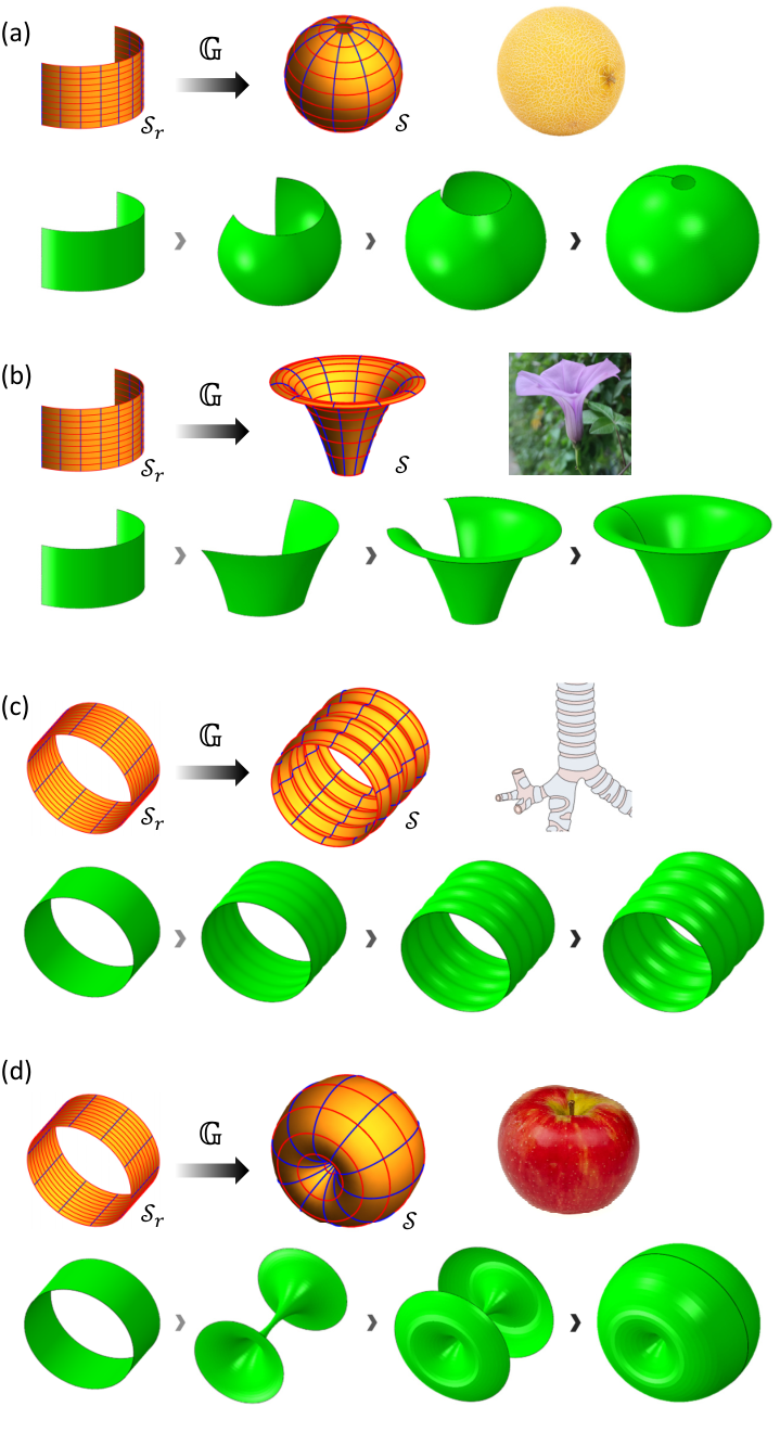
For concreteness, we consider four kinds of revolution surfaces inspired by biological tissues, i.e., the sweet melon, the morning glory, the trachea and the apple. The parametric equations and the corresponding growth functions of these surfaces are listed in (67)-(70). To verify the accuracy of the obtained growth functions, we also conduct numerical simulations by using the UMAT subroutine in ABAQUS, where the constitutive relation of a compressible neo-Hookean material is adopted. The Poisson’s ratio of the material is chosen to ν=0.4995\nu=0.4995 to capture the effect of elastic incompressibility. The growth functions λ1=λ1(0)+Z​λ1(1)\lambda_{1}=\lambda_{1}^{(0)}+Z\lambda_{1}^{(1)} and λ2=λ2(0)+Z​λ2(1)\lambda_{2}=\lambda_{2}^{(0)}+Z\lambda_{2}^{(1)} are incorporated as the state variables in UMAT, which change gradually from 11 to the target functions as those given in (67)-(70). The initial cylindrical shell has the dimensions R0=4R_{0}=4, h=0.01h=0.01 and l=4l=4. The value of Θ0\Theta_{0} is set to π\pi or 2​π2\pi depending upon the case. The whole sample is meshed into 20160 C3D8IH elements (8-node linear brick, hybrid, linear pressure, incompatible modes).

In Fig. 5, we show the numerical simulation results. It can be seen that the grown states of the shells are in good agreement with the target shapes. Thus, the correctness of the obtained growth functions can be verified. It should be pointed out here that we only try to mimic the shapes of the different biological tissues, but we do not aim to reveal the underlying mechanisms responsible for the growth of the biological tissues.
Refer to caption
Figure 5: Numerical simulation results on the growing processes of the shells with the target surfaces and growth functions listed in (67)-(70): (a) the sweet melon; (b) the morning glory; (c) the trachea; (d) the apple.
  • •

    Sweet melon (0≤θ1≤π,0≤θ2≤4):\left(0\leq\theta^{1}\leq\pi,\quad 0\leq\theta^{2}\leq 4\right):

{x(0)=4​cos⁡(2​θ1)​cos⁡(940​π​(θ2−2)),y(0)=4​sin⁡(2​θ1)​cos⁡(940​π​(θ2−2)),z(0)=−4​cos⁡(140​π​(9​θ2+2)),λ1=8cos(940π(θ2−2)),λ2=940π(Z+4).\left\{\begin{aligned} &x^{(0)}=4\cos(2{\theta^{1}})\cos\left(\frac{9}{40}\pi({\theta^{2}}-2)\right),\\ &y^{(0)}=4\sin(2{\theta^{1}})\cos\left(\frac{9}{40}\pi({\theta^{2}}-2)\right),\\ &z^{(0)}=-4\cos\left(\frac{1}{40}\pi(9{\theta^{2}}+2)\right),\\ &\lambda_{1}=8\cos\left(\frac{9}{40}\pi({\theta^{2}}-2)\right),\quad\lambda_{2}=\frac{9}{40}\pi(Z+4).\end{aligned}\right. (67)
  • •

    Morning glory (0≤θ1≤π,0≤θ2≤4)\left(0\leq\theta^{1}\leq\pi,\quad 0\leq{\theta^{2}}\leq 4\right)

{x(0)=−(1+θ2)​cos⁡(2​θ1),y(0)=−(1+θ2)​sin⁡(2​θ1),z(0)=6−18​(7−2​θ2)2,λ1=12​(θ2+1)​[4−4​(2​θ2−7)​Z(θ2+1)​4​θ2​(θ2−7)+53−Z],λ2=θ2​(θ2−7)+534−4​Z4​θ2​(θ2−7)+53.\left\{\begin{aligned} &x^{(0)}=-(1+{\theta^{2}})\cos(2\theta^{1}),\\ &y^{(0)}=-(1+{\theta^{2}})\sin(2\theta^{1}),\\ &z^{(0)}=6-\frac{1}{8}\left(7-2{\theta^{2}}\right)^{2},\\ &\lambda_{1}=\frac{1}{2}({\theta^{2}}+1)\left[4-\frac{4(2{\theta^{2}}-7)Z}{({\theta^{2}}+1)\sqrt{4{\theta^{2}}\left({\theta^{2}}-7\right)+53}}-Z\right],\\ &\lambda_{2}=\sqrt{{\theta^{2}}({\theta^{2}}-7)+\frac{53}{4}}-\frac{4Z}{4{\theta^{2}}\left({\theta^{2}}-7\right)+53}.\end{aligned}\right. (68)
  • •

    Trachea (0≤θ1≤2π,0≤θ2≤4)\left(0\leq\theta^{1}\leq 2\pi,\quad 0\leq{\theta^{2}}\leq 4\right)

{x(0)=15cosθ1[20+sin(2πθ2)],y(0)=15sinθ1[20+sin(2πθ2)],z(0)=2​(2+θ2),λ1=−120​(Z−4)​sin⁡(2​π​θ2)+4+Z⁡(5​2π2​cos⁡(4​π​θ2)+π2+50−1),λ2=15​2​π2​cos⁡(4​π​θ2)+π2+50+20​π2​Z​sin⁡(2​π​θ2)π2​cos⁡(4​π​θ2)+π2+50.\left\{\begin{aligned} &x^{(0)}=\frac{1}{5}\cos\theta^{1}\left[20+\sin(2\pi{\theta^{2}})\right],\\ &y^{(0)}=\frac{1}{5}\sin\theta^{1}\left[20+\sin(2\pi{\theta^{2}})\right],\\ &z^{(0)}=2(2+{\theta^{2}}),\\ &\lambda_{1}=-\frac{1}{20}(Z-4)\sin(2\pi{\theta^{2}})+4+Z\left(\frac{5\sqrt{2}}{\sqrt{\pi^{2}\cos(4\pi{\theta^{2}})+\pi^{2}+50}}-1\right),\\ &\lambda_{2}=\frac{1}{5}\sqrt{2}\sqrt{\pi^{2}\cos(4\pi{\theta^{2}})+\pi^{2}+50}+\frac{20\pi^{2}Z\sin(2\pi{\theta^{2}})}{\pi^{2}\cos(4\pi{\theta^{2}})+\pi^{2}+50}.\end{aligned}\right. (69)
  • •

    Apple (0≤θ1≤2π,0≤θ2≤4)\left(0\leq\theta^{1}\leq 2\pi,\quad 0\leq{\theta^{2}}\leq 4\right)

{x(0)=8cosθ1cos2(π​θ24),y(0)=8sinθ1cos2(π​θ24),z(0)=−6​sin⁡(π​θ22),λ1=−3​2​Z​cos⁡(π​θ22)5​cos⁡(π​θ2)+13−2​(Z−4)​cos2⁡(π​θ24),λ2=π⁡[5​cos⁡(π​θ2)+132−6​Z5​cos⁡(π​θ2)+13].\left\{\begin{aligned} &x^{(0)}=8\cos\theta^{1}\cos^{2}\left(\frac{\pi{\theta^{2}}}{4}\right),\\ &y^{(0)}=8\sin\theta^{1}\cos^{2}\left(\frac{\pi{\theta^{2}}}{4}\right),\\ &z^{(0)}=-6\sin\left(\frac{\pi{\theta^{2}}}{2}\right),\\ &\lambda_{1}=\frac{-3\sqrt{2}Z\cos\left(\frac{\pi{\theta^{2}}}{2}\right)}{\sqrt{5\cos(\pi{\theta^{2}})+13}}-2(Z-4)\cos^{2}\left(\frac{\pi{\theta^{2}}}{4}\right),\\ &\lambda_{2}=\pi\left[\frac{\sqrt{5\cos(\pi{\theta^{2}})+13}}{\sqrt{2}}-\frac{6Z}{5\cos(\pi{\theta^{2}})+13}\right].\end{aligned}\right. (70)

4.2 Example with change of variables

To further demonstrate the efficiency of the proposed theoretical scheme, we study two more examples, in which the target shapes are chosen to be the Cereus Forbesii Spiralis and the tendril of pumpkin.

Refer to caption
Figure 6: Change of variables between {θ1,θ2}\{\theta^{1},\theta^{2}\} and {η1,η2}\{\eta^{1},\eta^{2}\}, and the decomposition of the growth process for generating Cereus Forbesii Spiralis: (a) the original region Ωr\Omega_{r} on the parametric plane θ1​θ2\theta^{1}\theta^{2}; (b) the new region Ωr∗\Omega_{r}^{*} on the parametric plane η1​η2\eta^{1}\eta^{2}; (c) the base surface 𝒮r\mathcal{S}_{r} in the referential configuration 𝒦r\mathcal{K}_{r}, the base surface 𝒮i\mathcal{S}_{i} in the intermediate configuration 𝒦i\mathcal{K}_{i}, and the target base surface 𝒮\mathcal{S} in the current configuration 𝒦t\mathcal{K}_{t}; (d) the simulated growing process for generating the Cereus Forbesii Spiralis configuration of the shell.

For the case of Cereus Forbesii Spiralis, the parametric equation of the target surface 𝒮\mathcal{S} is

𝐱(0)​(θ1,θ2)={2​θ1π​sin⁡(π​θ2),2​θ1π​cos⁡(π​θ2),θ2},\mathbf{x}^{(0)}(\theta^{1},\theta^{2})=\left\{\frac{2\theta^{1}}{\pi}\sin(\pi{\theta^{2}}),\frac{2\theta^{1}}{\pi}\cos(\pi{\theta^{2}}),\theta^{2}\right\}, (71)

where the region of the parametric variable is chosen to be Ωr=[0,π]×[0,4]\Omega_{r}=[0,\pi]\times[0,4]. Corresponding to this parametric equation, one can obtain the first and second fundamental quantities as follows

E=4/π2,F=0,G=1+4θ12,\displaystyle E=4/\pi^{2},\quad F=0,\quad G=1+4{\theta^{1}}^{2}, (72)
L=0,M=2/1+4​θ12,N=0.\displaystyle L=0,\quad M=2/\sqrt{1+4{\theta^{1}}^{2}},\quad N=0.

As the quantity M≠0M\neq 0, we need to conduct the change of variables from (θ1,θ2)\left(\theta^{1},\theta^{2}\right) to (η1,η2)\left(\eta^{1},\eta^{2}\right). According to the procedure of variable change introduced in section 3.2, we have

η1​(θ1,θ2)=arcsinh​(2​θ1)π+θ2,η2​(θ1,θ2)=−arcsinh​(2​θ1)π+θ2.\eta^{1}\left(\theta^{1},{\theta^{2}}\right)=\frac{\text{arcsinh}(2\theta^{1})}{\pi}+{\theta^{2}},\quad\eta^{2}\left(\theta^{1},{\theta^{2}}\right)=-\frac{\text{arcsinh}(2\theta^{1})}{\pi}+{\theta^{2}}. (73)

After the variable transformation, the original region Ωr\Omega_{r} in the θ1​θ2\theta^{1}\theta^{2}- plane is mapped into a new region Ωr∗\Omega_{r}^{*} in the η1​η2\eta^{1}\eta^{2}-plane, which is shown in Fig. 6(b). On the region Ωr∗\Omega_{r}^{*}, a new surface 𝒮i\mathcal{S}_{i} is defined as follows

𝒮i:𝐬∗={R0cosη1,R0sinη1,η2},ηα∈Ωr∗.\mathcal{S}_{i}:\mathbf{s}^{*}=\{R_{0}\cos\eta^{1},R_{0}\sin\eta^{1},\eta^{2}\},\quad\eta^{\alpha}\in\Omega_{r}^{*}. (74)

Notice that the cylindrical shell 𝒮r\mathcal{S}_{r} defined by (61) and surface 𝒮i\mathcal{S}_{i} defined by (74) have the same parametric equation, but their parametric variable regions are different. As shown in Fig.(6)c, both 𝒮r\mathcal{S}_{r} and 𝒮i\mathcal{S}_{i} can be viewed as a subregion cutting from a large cylindrical surface with radius R0=4R_{0}=4. Also, the coordinate curves of {ηα}\{\eta^{\alpha}\} (i.e., the blue and red curves in Fig.6) constitute the orthogonal nets of curvature lines on both 𝒮i\mathcal{S}_{i} and 𝒮\mathcal{S}. By choosing 𝒮i\mathcal{S}_{i} as the base surface, we define an intermediate configuration 𝒦i\mathcal{K}_{i} according to (55), then the whole growth process can be divided into two steps: 𝒦r→𝒦i\mathcal{K}_{r}\rightarrow\mathcal{K}_{i} and from 𝒦i→𝒦t\mathcal{K}_{i}\rightarrow\mathcal{K}_{t}. For the first step, according to (56) the deformation gradient 𝔽0\mathbb{F}_{0} is given by

𝔽0=\displaystyle\mathbb{F}_{0}= 2π​1+4​θ12​𝐠1​(ηα)⊗𝐠1​(θα)+(1+Z/R0)​𝐠1​(ηα)⊗𝐠2​(θα)\displaystyle\frac{2}{\pi\sqrt{1+4{\theta^{1}}^{2}}}\mathbf{g}_{1}(\eta^{\alpha})\otimes\mathbf{g}^{1}(\theta^{\alpha})+(1+Z/R_{0})\mathbf{g}_{1}(\eta^{\alpha})\otimes\mathbf{g}^{2}(\theta^{\alpha}) (75)
−2π⁡(Z/R0+1)​1+4​θ12𝐠2(ηα)⊗𝐠1(θα)+𝐠2(ηα)⊗𝐠2(θα)+𝐧(ηα)⊗𝐧(θα).\displaystyle-\frac{2}{\pi\left(Z/R_{0}+1\right)\sqrt{1+4{\theta^{1}}^{2}}}\mathbf{g}_{2}(\eta^{\alpha})\otimes\mathbf{g}^{1}(\theta^{\alpha})+\mathbf{g}_{2}(\eta^{\alpha})\otimes\mathbf{g}^{2}(\theta^{\alpha})+\mathbf{n}(\eta^{\alpha})\otimes\mathbf{n}(\theta^{\alpha}).

For the second step, the growth tensor 𝔾1\mathbb{G}_{1} on domain (η1,η2)\left(\eta^{1},\eta^{2}\right) is obtained according to (57)

𝔾1=\displaystyle\mathbb{G}_{1}= 𝐠1(ηα)⊗𝐠1(ηα)[18cosh⁡(π⁡(η1−η2))+1\displaystyle\mathbf{g}_{1}(\eta^{\alpha})\otimes\mathbf{g}^{1}(\eta^{\alpha})\Bigg[\frac{1}{8}\sqrt{\cosh(\pi(\eta^{1}-\eta^{2}))+1} (76)
−Z⁡(16​π​cosh4⁡(12​π​(η1−η2))+cosh2⁡(π⁡(η1−η2))+2​cosh⁡(π⁡(η1−η2))+1)32​(cosh⁡(π⁡(η1−η2))+1)3/2]\displaystyle-\frac{Z\left(16\pi\sqrt{\cosh^{4}\left(\frac{1}{2}\pi(\eta^{1}-\eta^{2})\right)}+\cosh^{2}(\pi(\eta^{1}-\eta^{2}))+2\cosh(\pi(\eta^{1}-\eta^{2}))+1\right)}{32(\cosh(\pi(\eta^{1}-\eta^{2}))+1)^{3/2}}\Bigg]
+𝐠2(ηα)⊗𝐠2(ηα)[12cosh⁡(π⁡(η1−η2))+1+2​π​Z​cosh4⁡(12​π​(η1−η2))(cosh⁡(π⁡(η1−η2))+1)3/2]\displaystyle+\mathbf{g}_{2}(\eta^{\alpha})\otimes\mathbf{g}^{2}(\eta^{\alpha})\Big[\frac{1}{2}\sqrt{\cosh(\pi(\eta^{1}-\eta^{2}))+1}+\frac{2\pi Z\sqrt{\cosh^{4}\left(\frac{1}{2}\pi(\eta^{1}-\eta^{2})\right)}}{(\cosh(\pi(\eta^{1}-\eta^{2}))+1)^{3/2}}\Big]
+𝐧(ηα)⊗𝐧(ηα).\displaystyle+\mathbf{n}(\eta^{\alpha})\otimes\mathbf{n}(\eta^{\alpha}).

Then the tensor 𝔾\mathbb{G} generating the shape change from 𝒮r\mathcal{S}_{r} to 𝒮\mathcal{S} can be obtained according to (60). To verify the correctness of these growth functions, we simulate the growth process of Cereus Forbesii Spiralis in ABAQUS. The setting of the numerical simulations is the same as that introduced in the previous example. The numerical results of this case are shown in Fig. (6)d, which shows that the final shape of the shell can fit the target shape quite well.

For the case of pumpkin tendril, the parametric equation of the target surface 𝒮\mathcal{S} is

𝐱(0)​(θ1,θ2)={(cos⁡θ1+2)​cos⁡(π​θ22),(cos⁡θ1+2)​sin⁡(π​θ22),sin⁡θ1+θ2},\mathbf{x}^{(0)}(\theta^{1},\theta^{2})=\left\{(\cos\theta^{1}+2)\cos\left(\frac{\pi{\theta^{2}}}{2}\right),(\cos\theta^{1}+2)\sin\left(\frac{\pi{\theta^{2}}}{2}\right),\sin\theta^{1}+{\theta^{2}}\right\}, (77)

where the region on the parametric plane is chosen to be Ωr=[0,2​π]×[0,8]\Omega_{r}=[0,2\pi]\times[0,8]. Corresponding to this parametric equation, one can obtain the first and second fundamental quantities as follow

E=1,F=cosθ1,G=18(π2(8cos(θ1)+cos(2θ1))+9π2+8),\displaystyle E=1,\quad F=\cos\theta^{1},\quad G=\frac{1}{8}\left(\pi^{2}(8\cos({\theta^{1}})+\cos(2{\theta^{1}}))+9\pi^{2}+8\right), (78)
L=2​π​(cos⁡(θ1)+2)8​π2​cos⁡(θ1)+(π2−4)​cos⁡(2​θ1)+9​π2+4,\displaystyle L=\frac{\sqrt{2}\pi(\cos({\theta^{1}})+2)}{\sqrt{8\pi^{2}\cos({\theta^{1}})+\left(\pi^{2}-4\right)\cos(2{\theta^{1}})+9\pi^{2}+4}},
M=−2​π​sin2⁡(θ1)8​π2​cos⁡(θ1)+(π2−4)​cos⁡(2​θ1)+9​π2+4,\displaystyle M=-\frac{\sqrt{2}\pi\sin^{2}({\theta^{1}})}{\sqrt{8\pi^{2}\cos({\theta^{1}})+\left(\pi^{2}-4\right)\cos(2{\theta^{1}})+9\pi^{2}+4}},
N=π3​cos⁡(θ1)​(cos⁡(θ1)+2)22​2​8​π2​cos⁡(θ1)+(π2−4)​cos⁡(2​θ1)+9​π2+4.\displaystyle N=\frac{\pi^{3}\cos({\theta^{1}})(\cos({\theta^{1}})+2)^{2}}{2\sqrt{2}\sqrt{8\pi^{2}\cos({\theta^{1}})+\left(\pi^{2}-4\right)\cos(2{\theta^{1}})+9\pi^{2}+4}}.

Note that the quantities F≠0F\neq 0 and M≠0M\neq 0, thus the change of variables from (θ1,θ2)\left(\theta^{1},\theta^{2}\right) to (η1,η2)\left(\eta^{1},\eta^{2}\right) is required. As shown in Fig.7(b), the original region Ωr\Omega_{r} is mapped into a new region Ωr∗\Omega_{r}^{*} through the change of variables. Following the same parametric equation, these two regions define surfaces 𝒮r\mathcal{S}_{r} and 𝒮i\mathcal{S}_{i} respectively, where 𝒮r\mathcal{S}_{r} is a cylinder with radius R0=4R_{0}=4 and length l=8l=8, while 𝒮i\mathcal{S}_{i} is an irregular shaped subregion cut from a cylinder with radius R0=4R_{0}=4 as follow

𝒮i:𝐬∗={R0cosη1,R0sinη1,η2},ηα∈Ωr∗.\mathcal{S}_{i}:\mathbf{s}^{*}=\{R_{0}\cos\eta^{1},R_{0}\sin\eta^{1},\eta^{2}\},\quad\eta^{\alpha}\in\Omega_{r}^{*}. (79)

Also, the coordinate curves {ηα}\{\eta^{\alpha}\}(i.e., the blue and red curves in Fig.7) constitute an orthogonal curvature net on both 𝒮i\mathcal{S}_{i} and 𝒮\mathcal{S}. By choosing 𝒮i\mathcal{S}_{i} as the base surface, we define an intermediate configuration 𝒦i\mathcal{K}_{i}. The whole shape morphing process can be divided into two steps: from 𝒦r\mathcal{K}_{r} to 𝒦i\mathcal{K}_{i} described by 𝔽0\mathbb{F}_{0}, and the from 𝒦i\mathcal{K}_{i} to 𝒦t\mathcal{K}_{t} induced by 𝔾1\mathbb{G}_{1}. However, the analytical explicit expressions for integrating factors and (η1,η2)\left(\eta^{1},\eta^{2}\right) are difficult to obtain. Therefore the tensor 𝔽0\mathbb{F}_{0} and 𝔾1\mathbb{G}_{1} are calculated numerically in this case, and then the growth values are passed to the relating integration points on meshes in ABAQUS. According to the numerical results of this case shown in Fig.(7)(d), the final shapes fit the target shapes quite well.

Refer to caption
Figure 7: Change of variables between {θ1,θ2}\{\theta^{1},\theta^{2}\} and {η1,η2}\{\eta^{1},\eta^{2}\}, and the decomposition of the growth process for generating tendril of pumpkin: (a) the original region Ωr\Omega_{r} in the parametric plane θ1​θ2\theta^{1}\theta^{2}; (b) the new region Ωr∗\Omega_{r}^{*} in the parametric plane η1​η2\eta^{1}\eta^{2}; (c) the base surface 𝒮r\mathcal{S}_{r} in the referential configuration 𝒦r\mathcal{K}_{r}, the base surface 𝒮i\mathcal{S}_{i} on the intermediate configuration 𝒦i\mathcal{K}_{i}, and the target base surface 𝒮\mathcal{S} in the current configuration 𝒦t\mathcal{K}_{t}; (d) the simulated growing process for generating the tendril of pumpkin configuration of the shell.

5 Conclusions

The large deformations of thin hyperelastic shells induced by differential growth were investigated in this paper. To fulfill the goal of shape-programming of thin hyperelastic shells, the following tasks have been accomplished: (i) a consistent finite-strain shell equation system for modeling the growth-induced deformations of incompressible hyperelastic shells was formulated; (ii) the problem of shape-programming was solved analytically under the stress-free condition, from which the explicit expressions of the growth functions in terms of the geometrical quantities (i.e., the first and second fundamental forms) of the target surfaces were derived; (iii) a general theoretical scheme for shape-programming of thin hyperelastic shells through differential growth was proposed; (iv) to verify the correctness and efficiency of the scheme, some typical examples were studied, where the configurations of some biological tissues were simulated with the obtained growth functions.

Since the formulas derived in the current work have relatively simple forms and are valid for general incompressible hyperelastic material, the presented theoretical scheme for shape-programming would have wide potential applications for design and manufacturing of intelligent soft devices. Furthermore, the analytical results can also shed light on understanding the mechanical behaviors of some soft biological tissues in nature during the growth process. It should be noted that the current work still has some shortcomings that need to be tackled in future. One shortcoming is that the explicit expressions of growth tensor is derived based on the stress-free assumption, therefore, they are not valid for shell samples subjected to external loads or boundary restrictions. Additionally, the theoretical scheme is not applicable to complex 3D surfaces without explicit parametric equations. In that case, an efficient numerical scheme for shape-programming of complicated surfaces needs to be proposed.

Supplementary material

Movie 1: Growth process of shape-programming cases. Video of the growing processes of the six illustrative examples introduced in Fig. 5, 6 and 7 of the main text, which is available at https://github.com/Jeff97/growth-deformation-of-shell

Declaration of competing interest

The authors declare that they have no known competing financial interests or personal relationships that could have appeared to influence the work reported in this paper.

Acknowledgments

This work is supported by the National Natural Science Foundation of China (Project No.: 11872184). Z.L. is supported by the China Scholarship Council (CSC) Grant #202106150121. M.H. and Z. L. are indebted to the funding through an Engineering and Physical Sciences Research Council (EPSRC) Impact Acceleration Award (EP/R511614/1).

Appendix A Some results for incompressible Neo-Hookean material

To obtain some concrete results on the unknowns (𝐱(n)\mathbf{x}^{(n)} and p(n)p^{(n)}), we further assume that the shell is made of neo-Hookean material with the following elastic strain-energy function

ϕ⁡(𝔽,𝔾)=JG​ϕ0​(𝔸)=JG​C0​[tr⁡(𝔸​𝔸T)−3],\phi(\mathbb{F},\mathbb{G})=J_{G}\phi_{0}(\mathbb{A})=J_{G}C_{0}\left[\mathrm{tr}(\mathbb{A}\mathbb{A}^{T})-3\right], (A.1)

where C0C_{0} is a material constant. From the elastic strain-energy function ϕ⁡(𝔽,𝔾)\phi(\mathbb{F},\mathbb{G}), the nominal stress tensor 𝕊\mathbb{S} is given by

𝕊=JG​𝔾−1​(2​C0​𝔸T−p⁡(R,Z)​𝔸−1).\mathbb{S}=J_{G}\mathbb{G}^{-1}\left(2C_{0}\mathbb{A}^{T}-p(R,Z)\mathbb{A}^{-1}\right). (A.2)

For simplicity, we assume the shell is under traction-free condition. By taking series expansion on Z=0Z=0 and through some truncation manipulation, a closed linear system for {𝐱(1),𝐱(2),p(0),p(1)}\{\mathbf{x}^{(1)},\mathbf{x}^{(2)},p^{(0)},p^{(1)}\} is formulated by (23) and (24)1, combining with the boundary conditions (25)1. Then the following expressions of {𝐱(1),𝐱(2),p(0),p(1)}\{\mathbf{x}^{(1)},\mathbf{x}^{(2)},p^{(0)},p^{(1)}\} in terms of 𝐱(0)\mathbf{x}^{(0)} are solved

𝐱(1)=Λ​𝐱NΔ,p(0)=2​C0​Λ2Δ,\mathbf{x}^{(1)}=\Lambda\frac{\mathbf{x}_{N}}{\Delta},\quad p^{(0)}=2C_{0}\frac{\Lambda^{2}}{\Delta}, (A.3)
𝐱(2)=\displaystyle\mathbf{x}^{(2)}= 1Δ5/2​𝐱N​(Λ2​t9+Δ2Λ2​t8−Δ3/2​t1)−1Λ2​𝐚\displaystyle\frac{1}{{{\Delta^{5/2}}}}{\mathbf{x}_{N}}\left({{\Lambda^{2}}{t_{9}}+\frac{{{\Delta^{2}}}}{{{\Lambda^{2}}}}{t_{8}}-{\Delta^{3/2}}{t_{1}}}\right)-\frac{1}{{{\Lambda^{2}}}}{\mathbf{a}} (A.4)
+1Δ3​Λ3[𝐱(0),1(Λ4t5−Δ3λ2(0)t7)+𝐱(0),2(Λ4t4−Δ3λ1(0)t6)],\displaystyle+\frac{1}{{{\Delta^{3}}{\Lambda^{3}}}}\left[{{\mathbf{x}^{(0)}_{,1}}\left({{\Lambda^{4}}{t_{5}}-{\Delta^{3}}\lambda_{2}^{(0)}{t_{7}}}\right)+{\mathbf{x}^{(0)}_{,2}}\left({{\Lambda^{4}}{t_{4}}-{\Delta^{3}}\lambda_{1}^{(0)}{t_{6}}}\right)}\right],
p(1)=\displaystyle p^{(1)}= 2​C0​(1Λ​Δ​t8−2​ΛΔ​t1+Λ3Δ5/2​t9),\displaystyle 2C_{0}\left({\frac{1}{{\Lambda\sqrt{\Delta}}}{t_{8}}-\frac{{2\Lambda}}{\Delta}{t_{1}}+\frac{{{\Lambda^{3}}}}{{{\Delta^{5/2}}}}{t_{9}}}\right),

where

Λ=λ1(0)λ2(0),𝐱N=𝐱(0),1×𝐱(0),2,Δ=𝐱N⋅𝐱N,\displaystyle\Lambda=\lambda_{1}^{(0)}\lambda_{2}^{(0)},\quad\mathbf{x}_{N}=\mathbf{x}^{(0)}_{,1}\times\mathbf{x}^{(0)}_{,2},\quad\Delta=\mathbf{x}_{N}\cdot\mathbf{x}_{N},
Bα​β=𝐠α⋅𝐠β,α,𝐚=(λ1(0)2𝐱(0),2,2+λ2(0)2𝐱(0),1,1),\displaystyle B_{\alpha\beta}=\mathbf{g}_{\alpha}\cdot\mathbf{g}_{\beta,\alpha},\quad\mathbf{a}=\left({\lambda_{1}^{(0)}}^{2}\mathbf{x}^{(0)}_{,2,2}+{\lambda_{2}^{(0)}}^{2}\mathbf{x}^{(0)}_{,1,1}\right),
t1=(κ1+κ2)​Λ−λ1(1)​λ2(0)−λ1(0)​λ2(1),\displaystyle{\displaystyle t_{1}}=\left({{\kappa_{1}}+{\kappa_{2}}}\right)\Lambda-\lambda_{1}^{(1)}\lambda_{2}^{(0)}-\lambda_{1}^{(0)}\lambda_{2}^{(1)},
t2=(B11+B21)Λ,t3=(B12+B22)Λ,\displaystyle{\displaystyle t_{2}}=\left({{B_{11}}+{B_{21}}}\right)\Lambda,\quad{t_{3}}=\left({{B_{12}}+{B_{22}}}\right)\Lambda,
t4=Λ(Δ,1F−Δ,2E)+Δ[E(2Λ,2+t3)−F(2Λ,1+t2)],\displaystyle{\displaystyle t_{4}}=\Lambda\left({{\Delta_{,1}}F-{\Delta_{,2}}E}\right)+\Delta\left[{E\left({2{\Lambda_{,2}}+{t_{3}}}\right)-F\left({2{\Lambda_{,1}}+{t_{2}}}\right)}\right],
t5=Λ(Δ,2F−Δ,1G)+Δ[G(2Λ,1+t2)−F(2Λ,2+t3)],\displaystyle{\displaystyle t_{5}}=\Lambda\left({{\Delta_{,2}}F-{\Delta_{,1}}G}\right)+\Delta\left[{G\left({2{\Lambda_{,1}}+{t_{2}}}\right)-F\left({2{\Lambda_{,2}}+{t_{3}}}\right)}\right],
t6=λ1,2(0)Λ+λ1(0)(t3−λ2,2(0)λ1(0)),t7=λ2,1(0)Λ+λ2(0)(t2−λ1,1(0)λ2(0)),\displaystyle{\displaystyle t_{6}}=\lambda_{1,2}^{(0)}\Lambda+\lambda_{1}^{(0)}\left({{t_{3}}-\lambda_{2,2}^{(0)}\lambda_{1}^{(0)}}\right),\quad{t_{7}}=\lambda_{2,1}^{(0)}\Lambda+\lambda_{2}^{(0)}\left({{t_{2}}-\lambda_{1,1}^{(0)}\lambda_{2}^{(0)}}\right),
t8=(λ1(0)2N+λ2(0)2L),t9=(EN−2FM+GL).\displaystyle{\displaystyle t_{8}}=\left(\lambda_{1}^{{(0)}^{2}}N+\lambda_{2}^{{(0)}^{2}}L\right),\quad{t_{9}}=\left({EN-2FM+GL}\right).

The expressions of 𝕊(0)\mathbb{S}^{(0)} in terms of 𝐱(0)\mathbf{x}^{(0)} are obtained by substituting 𝐱(1)\mathbf{x}^{(1)} and p(0)p^{(0)} into (22)1

𝕊(0)=\displaystyle\mathbb{S}^{(0)}= 2C0𝐠1⊗[Λ3Δ2(F𝐱(0),2−G𝐱(0),1)+λ2(0)λ1(0)𝐱(0),1]\displaystyle 2C_{0}\mathbf{g}_{1}\otimes\left[\frac{\Lambda^{3}}{\Delta^{2}}(F\mathbf{x}^{(0)}_{,2}-G\mathbf{x}^{(0)}_{,1})+\frac{\lambda_{2}^{(0)}}{\lambda_{1}^{(0)}}\mathbf{x}^{(0)}_{,1}\right] (A.5)
+2C0𝐠2⊗[−Λ3Δ2(F𝐱(0),1−E𝐱(0),2)+λ1(0)λ2(0)𝐱(0),2].\displaystyle+2C_{0}\mathbf{g}_{2}\otimes\left[-\frac{\Lambda^{3}}{\Delta^{2}}(F\mathbf{x}^{(0)}_{,1}-E\mathbf{x}^{(0)}_{,2})+\frac{\lambda_{1}^{(0)}}{\lambda_{2}^{(0)}}\mathbf{x}^{(0)}_{,2}\right].

Accordingly, expression of 𝕊(1)\mathbb{S}^{(1)} is also obtained, where 𝐱(2)\mathbf{x}^{(2)} and p(1)p^{(1)} are kept for brevity

𝕊(1)=\displaystyle\mathbb{S}^{(1)}= 2C0𝐠1⊗[(−λ1(1)​λ2(0)+λ1(0)​λ2(1)+Λ​κ1)λ1(0)2𝐱(0),1−Λ2Δ𝐱(0),2×𝐱(2)\displaystyle 2C_{0}\mathbf{g}_{1}\otimes\Bigg[\frac{{\left({-\lambda_{1}^{(1)}\lambda_{2}^{(0)}+\lambda_{1}^{(0)}\lambda_{2}^{(1)}+\Lambda{\kappa_{1}}}\right)}}{\lambda_{1}^{(0)^{2}}}{\mathbf{x}^{(0)}_{,1}}-\frac{{{\Lambda^{2}}}}{\Delta}{\mathbf{x}^{(0)}_{,2}}\times{\mathbf{x}^{(2)}} (A.6)
+Λ4Δ5/2(N𝐱(0),1−M𝐱(0),2)+λ2(0)(ΔΛ,1−ΛΔ,1)Δ2​λ1(0)𝐱N\displaystyle+\frac{{{\Lambda^{4}}}}{{{\Delta^{5/2}}}}\left({N{\mathbf{x}^{(0)}_{,1}}-M{\mathbf{x}^{(0)}_{,2}}}\right)+\frac{{\lambda_{2}^{(0)}\left({\Delta{\Lambda_{,1}}-\Lambda{\Delta_{,1}}}\right)}}{{{\Delta^{2}}\lambda_{1}^{(0)}}}{\mathbf{x}_{N}}
−Λ⁡(κ2​Λ2+p(1)​Δ/(2​C0))Δ2(G𝐱(0),1−F𝐱(0),2)+λ2(0)2Δ𝐱N,1]\displaystyle-\frac{{\Lambda\left({{\kappa_{2}}{\Lambda^{2}}+{p^{(1)}}\Delta/(2{C_{0}})}\right)}}{{{\Delta^{2}}}}\left({G{\mathbf{x}^{(0)}_{,1}}-F{\mathbf{x}^{(0)}_{,2}}}\right)+\frac{\lambda_{2}^{(0)^{2}}}{\Delta}\mathbf{x}_{N,1}\Bigg]
+2C0𝐠2⊗[(λ1(1)​λ2(0)−λ1(0)​λ2(1)+Λ​κ2)λ2(0)2𝐱(0),2+Λ2Δ𝐱(0),1×𝐱(2)\displaystyle+2C_{0}\mathbf{g}_{2}\otimes\Bigg[\frac{{\left({\lambda_{1}^{(1)}\lambda_{2}^{(0)}-\lambda_{1}^{(0)}\lambda_{2}^{(1)}+\Lambda{\kappa_{2}}}\right)}}{{\lambda_{2}^{{{(0)}^{2}}}}}{\mathbf{x}^{(0)}_{,2}}+\frac{{{\Lambda^{2}}}}{\Delta}{\mathbf{x}^{(0)}_{,1}}\times{\mathbf{x}^{(2)}}
−Λ4Q5/2(M𝐱(0),1−L𝐱(0),2)+λ1(0)(ΔΛ,2−ΛΔ,2)Δ2​λ2(0)𝐱N\displaystyle-\frac{{{\Lambda^{4}}}}{{{Q^{5/2}}}}\left({M{\mathbf{x}^{(0)}_{,1}}-L{\mathbf{x}^{(0)}_{,2}}}\right)+\frac{{\lambda_{1}^{(0)}\left({\Delta{\Lambda_{,2}}-\Lambda{\Delta_{,2}}}\right)}}{{{\Delta^{2}}\lambda_{2}^{(0)}}}{\mathbf{x}_{N}}
+Λ⁡(κ1​Λ2+p(1)​Δ/(2​C0))Δ2(F𝐱(0),1−E𝐱(0),2)+λ1(0)2Δ𝐱N,2]\displaystyle+\frac{{\Lambda\left({{\kappa_{1}}{\Lambda^{2}}+{p^{(1)}}\Delta/(2{C_{0}})}\right)}}{{{\Delta^{2}}}}\left({F{\mathbf{x}^{(0)}_{,1}}-E{\mathbf{x}^{(0)}_{,2}}}\right)+\frac{{\lambda_{1}^{{{(0)}^{2}}}}}{\Delta}{\mathbf{x}_{N,2}}\Bigg]
+2C0𝐧⊗[(−Λ​t1Δ−p(1)/(2C0))𝐱N+Λ𝐱(2)\displaystyle+2C_{0}\mathbf{n}\otimes\Bigg[\left({-\frac{{\Lambda{t_{1}}}}{\Delta}-{p^{(1)}}/(2{C_{0}})}\right){\mathbf{x}_{N}}+\Lambda\mathbf{x}^{(2)}
+Λ2Δ3[(ΔΛ,1−ΛΔ,1)(G𝐱(0),1−F𝐱(0),2)−(ΔΛ,2−ΛΔ,2)(F𝐱(0),1−E𝐱(0),2)]\displaystyle+\frac{{{\Lambda^{2}}}}{{{\Delta^{3}}}}\left[{\left({\Delta{\Lambda_{,1}}-\Lambda{\Delta_{,1}}}\right)\left({G{\mathbf{x}^{(0)}_{,1}}-F{\mathbf{x}^{(0)}_{,2}}}\right)-\left({\Delta{\Lambda_{,2}}-\Lambda{\Delta_{,2}}}\right)\left({F{\mathbf{x}^{(0)}_{,1}}-E{\mathbf{x}^{(0)}_{,2}}}\right)}\right]
+Λ3Δ2(𝐱N,2×𝐱(0),1−𝐱N,1×𝐱(0),2)].\displaystyle+\frac{{{\Lambda^{3}}}}{{{\Delta^{2}}}}\left({{\mathbf{x}_{N,2}}\times{\mathbf{x}^{(0)}_{,1}}-{\mathbf{x}_{N,1}}\times{\mathbf{x}^{(0)}_{,2}}}\right)\Bigg].

Note that 𝕊(1)\mathbb{S}^{(1)} is also in terms of 𝐱(0)\mathbf{x}^{(0)} with the use of (A.4).

In order to fulfil the goal of shape-programming, growth functions {λ1(0),λ1(1),λ2(0),λ2(1)}\{\lambda_{1}^{(0)},\lambda_{1}^{(1)},\lambda_{2}^{(0)},\lambda_{2}^{(1)}\} of an arbitrary target shape 𝐱(0)\mathbf{x}^{(0)} need to be determined from shell equation system. Generally, the growth functions of a certain target shape may not be unique. To facilitate derivation, we assume all the components 𝕊(0)\mathbb{S}^{(0)} and 𝕊(1)\mathbb{S}^{(1)} in current configuration 𝒦t\mathcal{K}_{t} are zero. It is clear that, under the stress-free assumption, shell equation (28) and boundary conditions (29) are satisfied automatically.

First, all components of 𝕊(0)\mathbb{S}^{(0)} in (A.5) are set to be zero

{Λ3Δ2(F𝐱(0),2−G𝐱(0),1)+λ2(0)λ1(0)𝐱(0),1=𝟎,−Λ3Δ2(F𝐱(0),1−E𝐱(0),2)+λ1(0)λ2(0)𝐱(0),2=𝟎.\left\{\begin{aligned} &\frac{\Lambda^{3}}{\Delta^{2}}(F\mathbf{x}^{(0)}_{,2}-G\mathbf{x}^{(0)}_{,1})+\frac{\lambda_{2}^{(0)}}{\lambda_{1}^{(0)}}\mathbf{x}^{(0)}_{,1}=\mathbf{0},\\ -&\frac{\Lambda^{3}}{\Delta^{2}}(F\mathbf{x}^{(0)}_{,1}-E\mathbf{x}^{(0)}_{,2})+\frac{\lambda_{1}^{(0)}}{\lambda_{2}^{(0)}}\mathbf{x}^{(0)}_{,2}=\mathbf{0}.\\ \end{aligned}\right. (A.7)

For simplicity, we assume F=0F=0 in the current configuration, which means the moving frame {𝐱,1(0),𝐱,2(0),𝐱N}\{\mathbf{x}^{(0)}_{,1},\mathbf{x}^{(0)}_{,2},\mathbf{x}_{N}\} are perpendicular to each other. Then the equations (A.7) are simplified as

{(−GΛ3E2​G2+λ2(0)λ1(0))𝐱(0),1=𝟎,(−EΛ3E2​G2+λ1(0)λ2(0))𝐱(0),2=𝟎,\left\{\begin{aligned} &\left(-G\frac{\Lambda^{3}}{E^{2}G^{2}}+\frac{\lambda_{2}^{(0)}}{\lambda_{1}^{(0)}}\right)\mathbf{x}^{(0)}_{,1}=\mathbf{0},\\ &\left(-E\frac{\Lambda^{3}}{E^{2}G^{2}}+\frac{\lambda_{1}^{(0)}}{\lambda_{2}^{(0)}}\right)\mathbf{x}^{(0)}_{,2}=\mathbf{0},\\ \end{aligned}\right. (A.8)

where the relation Δ=E​G\Delta=EG is used. Subsequently, growth functions λ1(0)\lambda_{1}^{(0)} and λ2(0)\lambda_{2}^{(0)} are solved

λ1(0)=E,λ2(0)=G,\lambda_{1}^{(0)}=\sqrt{E},\quad\lambda_{2}^{(0)}=\sqrt{G}, (A.9)

where growth functions λ1(0)\lambda_{1}^{(0)} and λ2(0)\lambda_{2}^{(0)} just represent extension or shrinkage along the coordinate curves {θα}\{\theta^{\alpha}\} on 𝒮r\mathcal{S}_{r}.

Second, we consider all components of 𝕊(1)\mathbb{S}^{(1)} in (A.6) are zero

{(−λ1(1)​λ2(0)+λ1(0)​λ2(1)+Λ​κ1)λ1(0)2𝐱(0),1−Λ2Δ𝐱(0),2×𝐱(2)+Λ4Δ5/2(N𝐱(0),1−M𝐱(0),2)+λ2(0)(ΔΛ,1−ΛΔ,1)Δ2​λ1(0)𝐱N−Λ⁡(κ2​Λ2+p(1)​Δ/(2​C0))Δ2G𝐱(0),1+λ2(0)2Δ𝐱N,1=𝟎,(λ1(1)​λ2(0)−λ1(0)​λ2(1)+Λ​κ2)λ2(0)2𝐱(0),2+Λ2Δ𝐱(0),1×𝐱(2)−Λ4Q5/2(M𝐱(0),1−L𝐱(0),2)+λ1(0)(ΔΛ,2−ΛΔ,2)Δ2​λ2(0)𝐱N−Λ⁡(κ1​Λ2+p(1)​Δ/(2​C0))Δ2E𝐱(0),2+λ1(0)2Δ𝐱N,2=𝟎,(−Λ​t1Δ−p(1)/(2​C0))​𝐱N+Λ​𝐱(2)+Λ2Δ3[(ΔΛ,1−ΛΔ,1)G𝐱(0),1+(ΔΛ,2−ΛΔ,2)E𝐱(0),2]+Λ3Δ2(𝐱N,2×𝐱(0),1−𝐱N,1×𝐱(0),2)=𝟎.\left\{\begin{aligned} &\frac{{\left({-\lambda_{1}^{(1)}\lambda_{2}^{(0)}+\lambda_{1}^{(0)}\lambda_{2}^{(1)}+\Lambda{\kappa_{1}}}\right)}}{\lambda_{1}^{(0)^{2}}}{\mathbf{x}^{(0)}_{,1}}-\frac{{{\Lambda^{2}}}}{\Delta}{\mathbf{x}^{(0)}_{,2}}\times{\mathbf{x}^{(2)}}\\ &+\frac{{{\Lambda^{4}}}}{{{\Delta^{5/2}}}}\left({N{\mathbf{x}^{(0)}_{,1}}-M{\mathbf{x}^{(0)}_{,2}}}\right)+\frac{{\lambda_{2}^{(0)}\left({\Delta{\Lambda_{,1}}-\Lambda{\Delta_{,1}}}\right)}}{{{\Delta^{2}}\lambda_{1}^{(0)}}}{\mathbf{x}_{N}}\\ &-\frac{{\Lambda\left({{\kappa_{2}}{\Lambda^{2}}+{p^{(1)}}\Delta/(2{C_{0}})}\right)}}{{{\Delta^{2}}}}G{\mathbf{x}^{(0)}_{,1}}+\frac{\lambda_{2}^{(0)^{2}}}{\Delta}\mathbf{x}_{N,1}=\mathbf{0},\\ &\frac{{\left({\lambda_{1}^{(1)}\lambda_{2}^{(0)}-\lambda_{1}^{(0)}\lambda_{2}^{(1)}+\Lambda{\kappa_{2}}}\right)}}{{\lambda_{2}^{{{(0)}^{2}}}}}{\mathbf{x}^{(0)}_{,2}}+\frac{{{\Lambda^{2}}}}{\Delta}{\mathbf{x}^{(0)}_{,1}}\times{\mathbf{x}^{(2)}}\\ &-\frac{{{\Lambda^{4}}}}{{{Q^{5/2}}}}\left({M{\mathbf{x}^{(0)}_{,1}}-L{\mathbf{x}^{(0)}_{,2}}}\right)+\frac{{\lambda_{1}^{(0)}\left({\Delta{\Lambda_{,2}}-\Lambda{\Delta_{,2}}}\right)}}{{{\Delta^{2}}\lambda_{2}^{(0)}}}{\mathbf{x}_{N}}\\ &-\frac{{\Lambda\left({{\kappa_{1}}{\Lambda^{2}}+{p^{(1)}}\Delta/(2{C_{0}})}\right)}}{{{\Delta^{2}}}}E{\mathbf{x}^{(0)}_{,2}}+\frac{{\lambda_{1}^{{{(0)}^{2}}}}}{\Delta}{\mathbf{x}_{N,2}}=\mathbf{0},\\ &\left({-\frac{{\Lambda{t_{1}}}}{\Delta}-{p^{(1)}}/(2{C_{0}})}\right){\mathbf{x}_{N}}+\Lambda\mathbf{x}^{(2)}\\ &+\frac{{{\Lambda^{2}}}}{{{\Delta^{3}}}}\left[{\left({\Delta{\Lambda_{,1}}-\Lambda{\Delta_{,1}}}\right)G{\mathbf{x}^{(0)}_{,1}}+\left({\Delta{\Lambda_{,2}}-\Lambda{\Delta_{,2}}}\right)E{\mathbf{x}^{(0)}_{,2}}}\right]\\ &+\frac{{{\Lambda^{3}}}}{{{\Delta^{2}}}}\left({{\mathbf{x}_{N,2}}\times{\mathbf{x}^{(0)}_{,1}}-{\mathbf{x}_{N,1}}\times{\mathbf{x}^{(0)}_{,2}}}\right)=\mathbf{0}.\\ \end{aligned}\right. (A.10)

With the use of (A.9) and Δ=E​G\Delta=EG, (A.10)3 is automatically satisfied and (A.10)1 and (A.10)2 have the following form

{−(EN+G(2L−E(2κ1+κ2)+2Eλ1(1))+EGλ2(1))𝐱(0),1=ME𝐱(0),2,−(2EN+G(L−E(κ1+2κ2)+Eλ1(1))+2EGλ2(1))𝐱(0),2=ME𝐱(0),1.\left\{\begin{aligned} &-\left({EN+G\left({2L-E\left({2\kappa_{1}+\kappa_{2}}\right)+2\sqrt{E}\lambda_{1}^{(1)}}\right)+E\sqrt{G}\lambda_{2}^{(1)}}\right)\mathbf{x}^{(0)}_{,1}=ME{\mathbf{x}^{(0)}_{,2}},\\ &-\left({2EN+G\left({L-E\left({\kappa_{1}+2\kappa_{2}}\right)+\sqrt{E}\lambda_{1}^{(1)}}\right)+2E\sqrt{G}\lambda_{2}^{(1)}}\right){\mathbf{x}^{(0)}_{,2}}=ME{\mathbf{x}^{(0)}_{,1}}.\\ \end{aligned}\right. (A.11)

To ensure the holds of Eqs. (A.11), we need to set M=0M=0, which together with F=0F=0 assume that the coordinate curves {θα}\{\theta^{\alpha}\} formulate the orthogonal net of curvature lines on the target surface 𝒮t\mathcal{S}_{t}. Subsequently, the growth functions λ1(1)\lambda_{1}^{(1)} and λ2(1)\lambda_{2}^{(1)} are solved

λ1(1)=(κ1−LE)​E,λ2(1)=(κ2−NG)​G.\lambda_{1}^{(1)}=\left(\kappa_{1}-\frac{L}{E}\right)\sqrt{E},\quad\lambda_{2}^{(1)}=\left(\kappa_{2}-\frac{N}{G}\right)\sqrt{G}. (A.12)

It can be seen that the growth functions (A.9) and (A.12) are coincident with the results obtained in Section 3.1. Compared with the plate sample in Wang et al. 2022, a distinct feature of the current growth functions is that, the effects of curvature κ1\kappa_{1} and κ2\kappa_{2} are taken into account. By solving the problem of shape-programming of the Neo-Hookean shell, the relations between growth functions and geometric properties of the base surface 𝒮\mathcal{S} are also revealed.

References

  • Ambrosi et al. [2011] D Ambrosi, G. A. Ateshian, E. M. Arruda, S. C. Cowin, J Dumais, A Goriely, G. A. Holzapfel, J. D. Humphrey, R Kemkemer, and E Kuhl. Perspectives on biological growth and remodeling. Journal of the Mechanics and Physics of Solids, 59(4):863–883, 2011.
  • Liu et al. [2015] Z. S. Liu, W. Toh, and T. Y. Ng. Advances in mechanics of soft materials: a review of large deformation behavior of hydrogels. International Journal of Applied Mechanics, 07(05):1530001, 2015.
  • Goriely and Ben Amar [2005] Alain Goriely and Martine Ben Amar. Differential growth and instability in elastic shells. Physical Review Letters, 94(19):198103, 2005. doi:10.1103/PhysRevLett.94.198103.
  • Li et al. [2012] Bo Li, Yan-Ping Cao, Xi-Qiao Feng, and Huajian Gao. Mechanics of morphological instabilities and surface wrinkling in soft materials: a review. Soft matter, 8(21):5728, 2012. doi:10.1039/c2sm00011c.
  • Kempaiah and Nie [2014] Ravindra Kempaiah and Zhihong Nie. From nature to synthetic systems: shape transformation in soft materials. Journal of Materials Chemistry B, 2:2357–2368, 2014.
  • Huang et al. [2018] Changjin Huang, Zilu Wang, David Quinn, Subra Suresh, and K. Jimmy Hsia. Differential growth and shape formation in plant organs. Proceedings of the National Academy of Sciences of the United States of America, 115(49):12359–12364, 2018. doi:10.1073/pnas.1811296115.
  • Liu et al. [2016] Y. Liu, J. Genzer, and M. D. Dickey. “2d or not 2d”: shape-programming polymer sheets. Progress in Polymer Science, 52:79–106, 2016.
  • van Manen et al. [2018] Teunis van Manen, Shahram Janbaz, and Amir A. Zadpoor. Programming the shape-shifting of flat soft matter. Materials Today, 21(2):144–163, 2018. ISSN 13697021. doi:10.1016/j.mattod.2017.08.026.
  • Gladman et al. [2016] A. Sydney Gladman, Elisabetta A. Matsumoto, Ralph G. Nuzzo, L. Mahadevan, and Jennifer A. Lewis. Biomimetic 4d printing. Nature materials, 15(4):413–418, 2016. ISSN 1476-1122. doi:10.1038/nmat4544.
  • Siéfert et al. [2019] Emmanuel Siéfert, Etienne Reyssat, José Bico, and Benoît Roman. Bio-inspired pneumatic shape-morphing elastomers. Nature materials, 18(1):24–28, 2019. ISSN 1476-1122.
  • Tao et al. [2021] Ye Tao, Yi-Chin Lee, Haolin Liu, Xiaoxiao Zhang, Jianxun Cui, Catherine Mondoa, Mahnoush Babaei, Jasio Santillan, Guanyun Wang, Danli Luo, Di Liu, Humphrey Yang, Youngwook Do, Lingyun Sun, Wen Wang, Teng Zhang, and Lining Yao. Morphing pasta and beyond. Science advances, 7(19), 2021. doi:10.1126/sciadv.abf4098.
  • Hwang et al. [2022] Dohgyu Hwang, Edward J. Barron, A. B. M. Tahidul Haque, and Michael D. Bartlett. Shape morphing mechanical metamaterials through reversible plasticity. Science robotics, 7(63):eabg2171, 2022. doi:10.1126/scirobotics.abg2171.
  • Kondaurov and Nikitin [1987] V.I. Kondaurov and L.V. Nikitin. Finite strains of viscoelastic muscle tissue. Journal of Applied Mathematics and Mechanics, 51(3):346–353, 1987.
  • Rodriguez et al. [1994] Edward K. Rodriguez, Anne Hoger, and Andrew D. McCulloch. Stress-dependent finite growth in soft elastic tissues. Journal of Biomechanics, 27(4):455–467, 1994. ISSN 0021-9290. doi:10.1016/0021-9290(94)90021-3.
  • Ben Amar and Goriely [2005] Martine Ben Amar and Alain Goriely. Growth and instability in elastic tissues. Journal of the Mechanics and Physics of Solids, 53(10):2284–2319, 2005. ISSN 00225096. doi:10.1016/j.jmps.2005.04.008.
  • Wex et al. [2015] Cora Wex, Susann Arndt, Anke Stoll, Christiane Bruns, and Yuliya Kupriyanova. Isotropic incompressible hyperelastic models for modelling the mechanical behaviour of biological tissues: a review. Biomedizinische Technik. Biomedical engineering, 60(6):577–592, 2015. doi:10.1515/bmt-2014-0146.
  • Kadapa et al. [2021] Chennakesava Kadapa, Zhanfeng Li, Mokarram Hossain, and Jiong Wang. On the advantages of mixed formulation and higher-order elements for computational morphoelasticity. Journal of the Mechanics and Physics of Solids, 148:104289, 2021. doi:10.1016/j.jmps.2020.104289.
  • Li et al. [2011] Bo Li, Yan-Ping Cao, Xi-Qiao Feng, and Huajian Gao. Surface wrinkling of mucosa induced by volumetric growth: Theory, simulation and experiment. Journal of the Mechanics and Physics of Solids, 59(4):758–774, 2011. ISSN 00225096. doi:10.1016/j.jmps.2011.01.010.
  • Goriely [2017] A. Goriely. The Mathematics and Mechanics of Biological Growth. Springer, New York, NY, 2017.
  • Pezzulla et al. [2018] Matteo Pezzulla, Norbert Stoop, Mark P. Steranka, Abdikhalaq J. Bade, and Douglas P. Holmes. Curvature-induced instabilities of shells. Physical review letters, 120(4):048002, 2018. doi:10.1103/PhysRevLett.120.048002.
  • Xu et al. [2020] Fan Xu, Chenbo Fu, and Yifan Yang. Water affects morphogenesis of growing aquatic plant leaves. Physical review letters, 124(3):038003, 2020. doi:10.1103/PhysRevLett.124.038003.
  • Dias et al. [2011] M.A. Dias, J.A. Hanna, and C.D. Santangelo. Programmed buckling by controlled lateral swelling in a thin elastic sheet. Physical Review E, 84:036603, 2011.
  • Jones and Mahadevan [2015] G. W. Jones and L. Mahadevan. Optimal control of plates using incompatible strains. Nonlinearity, 28(9):3153–3174, 2015.
  • Acharya [2019] Amit Acharya. A design principle for actuation of nematic glass sheets. Journal of Elasticity, 136:237–249, 2019.
  • Wang et al. [2019a] Jiong Wang, Qiongyu Wang, Hui-Hui Dai, Ping Du, and Danxian Chen. Shape-programming of hyperelastic plates through differential growth: an analytical approach. Soft Matter, 15(11):2391–2399, 2019a.
  • Nojoomi et al. [2021] A. Nojoomi, J. Jeon, and K. Yum. 2d material programming for 3d shaping. Nature Communications, 12:603, 2021.
  • Li et al. [2022] Zhanfeng Li, Qiongyu Wang, Ping Du, Chennakesava Kadapa, Mokarram Hossain, and Jiong Wang. Analytical study on growth-induced axisymmetric deformations and shape-control of circular hyperelastic plates. International Journal of Engineering Science, 170(31):103594, 2022. ISSN 00207225. doi:10.1016/j.ijengsci.2021.103594.
  • Wang et al. [2022] Jiong Wang, Zhanfeng Li, and Zili Jin. A theoretical scheme for shape-programming of thin hyperelastic plates through differential growth. Mathematics and Mechanics of Solids, page 108128652210896, 2022. ISSN 1081-2865. doi:10.1177/10812865221089694.
  • Vetter et al. [2013] Roman Vetter, Norbert Stoop, Thomas Jenni, Falk K. Wittel, and Hans J. Herrmann. Subdivision shell elements with anisotropic growth. International Journal for Numerical Methods in Engineering, 95(9):791–810, 2013. ISSN 00295981. doi:10.1002/nme.4536.
  • Rausch and Kuhl [2014] Manuel K. Rausch and Ellen Kuhl. On the mechanics of growing thin biological membranes. Journal of the Mechanics and Physics of Solids, 63:128–140, 2014. ISSN 00225096. doi:10.1016/j.jmps.2013.09.015.
  • Souhayl Sadik et al. [2016] Souhayl Sadik, Arzhang Angoshtari, Alain Goriely, and Arash Yavari. A geometric theory of nonlinear morphoelastic shells. Journal of Nonlinear Science, 26(4):929–978, 2016. ISSN 1432-1467. doi:10.1007/s00332-016-9294-9.
  • Song and Dai [2016] Zilong Song and Hui-Hui Dai. On a consistent finite-strain shell theory based on 3-d nonlinear elasticity. International Journal of Solids and Structures, 97-98:137–149, 2016. ISSN 00207683. doi:10.1016/j.ijsolstr.2016.07.034.
  • Yu et al. [2022] Xiang Yu, Xiang Zhong, and Xiaoyi Chen. On an asymptotic shell model for growth-induced finite deformations. unpublished results, 2022.
  • Ciarlet [2005] Philippe G. Ciarlet. An introduction to differential geometry with applications to elasticity. Journal of Elasticity, 78(1):1–215, 2005. ISSN 1573-2681. doi:10.1007/s10659-005-4738-8.
  • Steigmann [2012] David J. Steigmann. Extension of koiter’s linear shell theory to materials exhibiting arbitrary symmetry. International Journal of Engineering Science, 51:216–232, 2012. ISSN 00207225. doi:10.1016/j.ijengsci.2011.09.012.
  • Chen [2017] W. H. Chen. Differential geometry (2nd Edition). Peking University Press, 2017.
  • Groh [2022] Rainer M.J. Groh. A morphoelastic stability framework for post-critical pattern formation in growing thin biomaterials. Computer Methods in Applied Mechanics and Engineering, 394:114839, 2022. ISSN 0045-7825. doi:https://doi.org/10.1016/j.cma.2022.114839.
  • Dortdivanlioglu et al. [2017] Berkin Dortdivanlioglu, Ali Javili, and Christian Linder. Computational aspects of morphological instabilities using isogeometric analysis. Computer Methods in Applied Mechanics and Engineering, 316:261–279, 2017. ISSN 0045-7825. doi:https://doi.org/10.1016/j.cma.2016.06.028.
  • Mehta et al. [2021] Sumit Mehta, Gangadharan Raju, and Prashant Saxena. Growth induced instabilities in a circular hyperelastic plate. International Journal of Solids and Structures, 226-227:111026, 2021. ISSN 0020-7683. doi:https://doi.org/10.1016/j.ijsolstr.2021.03.013.
  • Dai and Song [2014] Hui-Hui Dai and Zilong Song. On a consistent finite-strain plate theory based on three-dimensional energy principle. Proceedings of the Royal Society A: Mathematical, Physical and Engineering Sciences, 470:20140494, 2014.
  • Wang et al. [2016] Jiong Wang, Zilong Song, and Hui-Hui Dai. On a consistent finite-strain plate theory for incompressible hyperelastic materials. International Journal of Solids and Structures, 78-79:101–109, 2016. ISSN 00207683.
  • Wang et al. [2018] Jiong Wang, David Steigmann, Fan-Fan Wang, and Hui-Hui Dai. On a consistent finite-strain plate theory of growth. Journal of the Mechanics and Physics of Solids, 111:184–214, 2018. ISSN 00225096.
  • Toponogov [2006] V. A. Toponogov. Differential geometry of curves and surfaces. Birkhäuser Boston, 2006.
  • Wang et al. [2019b] Jiong Wang, Qiongyu Wang, Hui-Hui Dai, Ping Du, and Danxian Chen. Shape-programming of hyperelastic plates through differential growth: an analytical approach. Soft matter, 15(11):2391–2399, 2019b. doi:10.1039/c9sm00160c.