On the Importance of Gradient Norm in PAC-Bayesian Bounds

Itai Gat Affiliation: Technion Yossi Adi Affiliation: FAIR Team, Meta AI Research Affiliation: The Hebrew University of Jerusalem Alexander Schwing Affiliation: University of Illinois at Urbana-Champaign Tamir Hazan Affiliation: Technion

Abstract

Generalization bounds which assess the difference between the true risk and the empirical risk have been studied extensively. However, to obtain bounds, current techniques use strict assumptions such as a uniformly bounded or a Lipschitz loss function. To avoid these assumptions, in this paper, we follow an alternative approach: we relax uniform bounds assumptions by using on-average bounded loss and on-average bounded gradient norm assumptions. Following this relaxation, we propose a new generalization bound that exploits the contractivity of the log-Sobolev inequalities. These inequalities add an additional loss-gradient norm term to the generalization bound, which is intuitively a surrogate of the model complexity. We apply the proposed bound on Bayesian deep nets and empirically analyze the effect of this new loss-gradient norm term on different neural architectures.

1 Introduction

Deep neural networks are ubiquitous across disciplines and often achieve state-of-the-art results. Despite the fact that deep nets are able to encode highly complex input-output relations, in practice, they do not tend to overfit (Zhang et al. 2016). This tendency to not overfit has been investigated in numerous works on generalization bounds. Indeed, many generalization bounds apply to composite functions specified by deep nets. However, most of these results assume that the loss function satisfies various assumptions, such as uniformly bounded (Alquier et al. 2016), Lipschitz (Alquier et al. 2019), sub-Gaussian (Bégin et al. 2016; Alquier and Guedj 2018), sub-gamma (Germain et al. 2016), or self-bounding (Haddouche et al. 2021). Unfortunately, these assumptions exclude many state-of-the-art deep nets, whose properties cannot be statistically determined per data distribution.

In this work, we take a different route and use the deep net gradient-norm as a measure for PAC-Bayesian generalization. For this purpose, we treat the loss function as a random function that is generated by a high-dimensional probability space, which is governed by the generating process of the training data. This view allows us to introduce new tools from high-dimensional probability theory that relate measure concentration to expansion of the loss function, as determined by its gradient-norm (van Handel 2016).

We begin by adjusting a theorem (Herbst theorem) to estimate the measure concentration via the entropy of the loss function (Lemma 3.1). We then derive a term for the entropy tailored to the multiclass classification setting (discrete labels which condition Gaussian data), (Lemma 3.2). Finally we bound the entropy using a log-Sobolev inequality (Lemma 3.3).

Importantly, these steps result in a PAC-Bayesian bound which depends on the norm of the gradient of the loss. Intuitively this norm measures the complexity of the loss function, i.e., the model. Different from prior work, the bound hence depends on the structure of the employed model and its gradient norm. This result admits a bound for multi-class classification with linear models and Lipschitz loss (Theorem 3.4), extending a result of Alquier et al. 2016, and multi-class classification with deep nets when the loss function and its gradient are on-average bounded (Theorem 3.5 and Theorem 3.6). The assumptions for the derived bound (Theorem 3.5 and Theorem 3.6) are closer to present-day deep net practice emphasizing the importance of the gradients in learning: in addition to the critical importance of controlling the loss gradient to better optimize a deep net, the gradient-norm also controls the generalization of the loss function (as measured by the deep net).

Our contributions: (1) We present a new PAC-Bayesian generalization bound that depends on the gradient-norm of the loss function. Consequently, we replace the uniform bound assumptions with an on-average bounded loss and an on-average bounded gradient norm. This answers an open problem raised by Bartlett et al. 2017a (cf. Sec. 4) in the PAC-Bayesian setting. This result is presented in Theorem 3.5. (2) We extend the PAC-Bayesian bounds of Alquier et al. 2016 for the hinge-loss to any linear model with a Lipschitz loss function. This result appears in Theorem 3.4. (3) We empirically demonstrate that our bounds produce tighter generalization performance than the baseline methods. This helps to bridge the gap between theory and practice towards tighter bounds that have more realistic assumptions that match modern deep nets.

2 Background

Generalization bounds provide statistical guarantees on learning algorithms. They assess how the learned parameters $w$ of a model perform on test data given the model’s result on the training data $S=\{(x_{1},y_{1}),\ldots,(x_{m},y_{m})\}$ , where $x_{i}$ is the data instance and $y_{i}$ is the corresponding label. The performance of the parametric model is measured by a loss function $\ell(w,x,y)$ . The risk $L_{D}(w)=\E_{(x,y)\sim D}\ell(w,x,y)$ of this model is its average loss, when the data instance and its label are sampled from the true but unknown distribution $D$ . The empirical risk is the average training set loss $L_{S}(w)=\frac{1}{m}\sum_{i=1}^{m}\ell(w,x_{i},y_{i})$ .

2.1 PAC-Bayesian bounds

PAC-Bayesian theory bounds the expected risk $\E_{w\sim q}L_{D}(w)$ of a model when its parameters are averaged over the learned posterior distribution $q$ . The posterior distribution is learned from the training data $S$ . In our work, we start from the following PAC-Bayesian bound:

Theorem 2.1 (Alquier et al. 2016).

Let $KL(q||p)=\int q(w)\log(q(w)/p(w))dw$ be the KL-divergence between two probability density functions $p,q$ . For any $\lambda>0$ , for any $\delta\in(0,1)$ and for any prior distribution $p$ , with probability at least $1-\delta$ over the draw of the training set $S$ , the following holds simultaneously for any posterior distribution $q$ :

\E_{w\sim q}[L_{D}(w)]\leq\E_{w\sim q}[L_{S}(w)]+\frac{1}{\lambda}[C(\lambda,p)+KL(q||p)+\log(1/\delta)],

(1)

where $C(\lambda,p)\triangleq\log\Big(\E_{w\sim p,S\sim D^{m}}[e^{\lambda(L_{D}(w)-L_{S}(w))}]\Big).$

Unfortunately, the complexity term $C(\lambda,p)$ of this bound is challenging to compute exactly in general: it requires to integrate (and maximize if the log-sum-exp trick is used) over large parameter and data spaces. Using different assumptions, e.g., learning with sub-Gaussian or sub-gamma loss functions, learning with specific losses, etc., it is possible to analytically bound the complexity term $C(\lambda,p)$ as we briefly illustrate next.

We say that a loss function $\ell$ is sub-Gaussian with variance $\nu^{2}$ if it can be described by a sub-Gaussian random variable, i.e., if its log-moment generating function is upper bounded by $\nu^{2}/2$ :

\displaystyle\log\Big(\E_{(x,y)\sim D}[e^{\lambda(L_{D}(w)-\ell(w,x,y))}]\Big)\leq\frac{\lambda^{2}\nu^{2}}{2}.

(2)

Alquier et al. 2016 use Hoeffding’s lemma to show that a uniformly bounded loss function, namely $0\leq\ell(w,x,y)\leq B$ is a sub-Gaussian loss function with variance $B^{2}$ and hence derive from Theorem 2.1 and Equation (2) a PAC-Bayesian bound for bounded loss functions.

2.2 Measure concentration in high-dimension

However, the Hoeffding lemma, which asserts the sub-Gaussian property to a bounded loss function, treats the value of the loss as a real-valued random variable $\ell(w,x,y)$ while entirely ignoring the high-dimensional probability space $(x,y)$ that generates this random value. Said differently: any properties of a function $F$ transforming the data $(x,y)$ are ignored, and all functions $F$ are treated identically. This is sub-optimal. In the following, we describe an entropy method that utilizes the measure concentration phenomena that exist in the high-dimensional random space of $(x,y)$ , cf. Chapter 3 of van Handel 2016. The entropy of a non-negative random variable $F$ is

\displaystyle\ent[F]\triangleq\E[F\log F]-\E[F]\log\E[F].

(3)

The Herbst theorem connects $\ent[F]$ to measure concentration by providing a bound on the log-moment generating function, as summarized next.

Theorem 2.2 (Herbst).

Suppose that for all $\lambda>0$ the following bound for the entropy holds:

\displaystyle\ent[e^{\lambda F}]\leq\frac{\lambda^{2}\sigma^{2}}{2}\E[e^{\lambda F}].

(4)

Then the scaled log-moment generating function which we also refer to as $\psi(\lambda)/\lambda$ is bounded as follows:

\displaystyle\frac{\psi(\lambda)}{\lambda}\triangleq\frac{1}{\lambda}\log\Big(\E[e^{\lambda F}]\Big)\leq\E[F]+\frac{\lambda\sigma^{2}}{2}.

(5)

Proof.

First we note that due to the fundamental theorem of calculus

\displaystyle\frac{\psi(\lambda)}{\lambda}=\frac{\psi(0)}{0}+\int_{0}^{\lambda}\left(\frac{\psi(\alpha)}{\alpha}\right)^{\prime}d\alpha.

(6)

Using l’Hopital rule, we verify that $\lim_{\alpha\rightarrow 0}\frac{\psi(\alpha)}{\alpha}=\E[F]$ , which yields the first term of the bound. The following identity

\displaystyle\left(\frac{\psi(\alpha)}{\alpha}\right)^{\prime}=\frac{\ent[e^{\alpha F}]}{\alpha^{2}\E[e^{\alpha F}]},

(7)

which is obtained from the definition of $\psi(\alpha)/\alpha$ and where $(\cdot)^{\prime}$ refers to the derivative w.r.t. $\alpha$ , derives the theorem after plugging Equation (7) into Equation (6) and using Equation (4) to bound the integral. ∎

Importantly, note that this is a step forward. Different from classical PAC-Bayesian bounds discussed in Section 2.1, which use the fact that a uniformly bounded loss function is sub-Gaussian, the Herbst theorem asserts that any random variable that satisfies Equation (4) is $\sigma^{2}$ sub-Gaussian.

To take advantage of this step, in this work, we benefit from the (modified) log-Sobolev inequality (LSI) for Gaussian random variables, which bounds the entropy.

Theorem 2.3 (Gaussian log-Sobolev inequality (LSI), Gross 1975).

Let $Z_{1},...,Z_{d}$ be independent Gaussian random variables, i.e., $Z_{i}\sim{\cal N}(\mu_{i},\sigma_{i}^{2})$ . We then have

\ent_{\cal N}[e^{f(Z_{1},...,Z_{d})}]\leq\frac{1}{2}\E_{\cal N}[\|\sigma\cdot\nabla_{Z}f(Z_{1},...,Z_{d})\|^{2}e^{f(Z_{1},...,Z_{d})}],

(8)

where $\sigma\cdot\nabla_{Z}f(Z_{1},...,Z_{d})$ is an element-wise multiplication.

Proof.

See supplementary material, Appendix A. ∎

One can apply the LSI to the Herbst theorem to attain measure concentration bounds for high-dimensional Lipschitz functions: a differentiable function $f(z_{1},...,z_{d})$ is said to be $g$ -Lipschitz if $|f(z_{1},...,z_{d})-f(z^{\prime}_{1},...,z^{\prime}_{d})|\leq g\|z-z^{\prime}\|$ , or equivalently, if $\|\nabla f(z_{1},...,z_{d})\|\leq g$ for any $z_{1},...,z_{d}$ . The LSI for $g$ -Lipschitz functions with $s\triangleq\sum_{i=1}^{d}\sigma_{i}^{2}$ variance reduces to the bound $\ent[e^{\lambda f(z_{1},...,z_{d})}]\leq\frac{\lambda^{2}g^{2}s}{2}\E[e^{\lambda f(z_{1},...,z_{d})}]$ , which in turn provides a bound on the log-moment generating function of $f(z_{1},...,z_{d})$ using Theorem 2.2.

3 PAC-Bayesian bounds with log-Sobolev inequalities

Different from prior work, we suggest to measure the generalization of neural nets by taking into account the expected gradient-norm of the loss function with respect to the data generation process.

For this we note that classical PAC-Bayesian generalization bounds depend on measure concentration, as described in Theorem 2.1 and Equation (2.1). However, the sub-Gaussian assumption used in classical PAC-Bayesian generalization bounds seamlessly bypasses the measure concentration phenomena. This is too restrictive and enforces all loss functions, and consequently all neural nets, to have the same measure concentration phenomena.

Instead, we first use the Herbst theorem to estimate the measure concentration by taking into account the entropy. In a second step we use Log-Sobolev inequalities (LSI) to bound the entropy, which allows us to consider the high-dimensional probability space $(x,y)\sim\D$ that controls the measure concentration of the loss function $\ell(w,x,y)$ . This differs from the use of a crude worst-case bound on the loss function (e.g., $\ell(w,x,y)\leq B$ for any $w,x,y$ ) in classical PAC-Bayesian generalization bounds, which entirely ignores the neural net that generates the loss function.

1) Herbst theorem to estimate measure concentration: As just discussed, we first adjust the Herbst theorem to our setting:

Lemma 3.1 (Herbst).

For any $\lambda>0$ we have

\displaystyle\log\left(\E_{S\sim\D^{m}}\big[e^{\lambda(L_{D}(w)-L_{S}(w))}\big]\right)=\lambda\int_{0}^{\frac{\lambda}{m}}\frac{\ent_{\D}[e^{-\alpha\ell(w,x,y)}]}{\alpha^{2}\E_{\D}[e^{-\alpha\ell(w,x,y)}]}d\alpha.

(9)

Proof.

First, we use the statistical independence of the training samples to decompose the moment generating function

\displaystyle M\left(\lambda\right)\triangleq E_{(x,y)\sim\D}[e^{\lambda(-\ell(w,x,y))}]

(10)

as follows:

$\displaystyle\E_{S\sim\D^{m}}\big[e^{\lambda(L_{D}(w)-L_{S}(w))}\big]$	$\displaystyle=$	$\displaystyle e^{\lambda L_{D}(w)}\E_{S\sim\D^{m}}[e^{\lambda\frac{1}{m}\sum_{i=1}^{m}(-\ell(w,x_{i},y_{i}))}]$	(11)
	$\displaystyle=$	$\displaystyle e^{\lambda L_{D}(w)}\prod_{i=1}^{m}\E_{(x_{i},y_{i})\sim\D}[e^{\frac{\lambda}{m}(-\ell(w,x_{i},y_{i}))}]$	(12)
	$\displaystyle=$	$\displaystyle e^{\lambda L_{D}(w)}M\left(\frac{\lambda}{m}\right)^{m}.$	(13)

We apply the differential representation of Theorem 2.2 with $\psi(\lambda)=\log M\left(\lambda\right)$ and obtain:

\displaystyle\frac{\psi(\lambda)}{\lambda}=\int_{0}^{\lambda}\left(\frac{\psi(\alpha)}{\alpha}\right)^{\prime}d\alpha+\frac{\psi(0)}{0}=\int_{0}^{\lambda}\frac{\ent_{\D}[e^{-\alpha\ell(w,x,y)}]}{\alpha^{2}\E_{\D}[e^{-\alpha\ell(w,x,y)}]}d\alpha-\E_{(x,y)\sim\D}[\ell(w,x,y)].

(14)

Since $M\left(\lambda/m\right)=e^{\psi(\lambda/m)}$ and $\E_{(x,y)\sim\D}[\ell(w,x,y)]=L_{D}(w)$ , we obtain from Equation (14) the identity

M\left(\frac{\lambda}{m}\right)^{m}=e^{\lambda\int_{0}^{\frac{\lambda}{m}}\frac{\ent_{\D}[e^{-\alpha\ell(w,x,y)}]}{\alpha^{2}\E_{\D}[e^{-\alpha\ell(w,x,y)}]}d\alpha-\lambda L_{D}(w)},

(15)

which completes the proof when being combined with Equation (13). ∎

2) Entropy bound: In the second step we now aim to bound the entropy $\ent_{\D}[e^{-\alpha\ell(w,x,y)}]$ .

Since we focus on the classification setting, the label $y$ is discrete. We further assume that for any (discrete) label $y$ its corresponding data $x=(x_{1},...,x_{d})$ is generated from a $d$ -dimensional Gaussian distribution that consists of $d$ i.i.d. Gaussian random variables $x_{i}\sim{\cal N}(\mu_{y,i},\sigma_{y,i}^{2})$ . We denote this Gaussian distribution by $x\sim{\cal N}(\mu_{y},\sigma_{y}^{2})$ and abbreviate it by $x\sim{\cal N}_{y}$ . The data generation distribution of $x$ is the Gaussian mixture model $\D=\sum_{y}\D_{y}\cdot{\cal N}_{y}$ , where $\D_{y}$ is the marginal distributions of $\D$ w.r.t $y$ .

We begin by decomposing the entropy of the (exponent) of the loss function according to the labels:

Lemma 3.2.

Let $\D=\sum_{y}D_{y}\cdot{\cal N}_{y}$ be a mixture model, whose label marginal probabilities are $D_{y}$ and set $f_{w}(x,y)=e^{-\alpha\ell(w,x,y)}$ . One can show that

\displaystyle\ent_{\D}[f_{w}]=\sum_{y}D_{y}\ent_{\N_{y}}[f_{w}]+\ent_{\D_{y}}[\E_{x\sim\N_{y}}[f_{w}]].

(16)

Proof.

From the definition of the entropy of a function $\ell(w,x,y)$ with respect to its measure $(x,y)\sim\D$ we have

\displaystyle\ent_{\D}[f]\triangleq\E_{\D}f_{w}(x,y)\log f_{w}(x,y)-\left(\E_{\D}[f_{w}(x,y)]\right)\log\left(\E_{\D}[f_{w}(x,y)]\right).

(17)

The result is attained by adding and subtracting the quantity $\E_{y\sim\D}\left(\E_{x\sim{\cal N}_{y}}[f_{w}(x,y)]\right)\log\left(\E_{x\sim{\cal N}_{y}}[f_{w}(x,y)]\right)$ . The result then follows from the definitions of entropies of the mixed components, while setting $g(y)=\E_{x\sim{\cal N}_{y}}[f_{w}(x,y)]$ . Specifically we have

	$\displaystyle\ent_{\N_{y}}[f_{w}]$	$\displaystyle\triangleq$	$\displaystyle\E_{\N_{y}}[f_{w}(x,y)\log f_{w}(x,y)]-\left(\E_{\N_{y}}[f_{w}(x,y)]\right)\log\left(\E_{\N_{y}}[f_{w}(x,y)]\right),$		(18)
	$\displaystyle\ent_{\D_{y}}[g]$	$\displaystyle\triangleq$	$\displaystyle\sum_{y}D_{y}g(y)\log(g(y))-\left(\sum_{y}D_{y}g(y)\right)\log\left(\sum_{y}D_{y}g(y)\right).$		(19)

∎

It is important to note that the number of components in the mixture model is not limited. Such a Gaussian mixture model can approximate any smooth density (Titterington et al. 1985; Scott 1992; Goodfellow et al. 2016).

Next, we use the LSI to bound the loss function entropy using its expected gradient-norm with respect to the data generation process.

Lemma 3.3.

Assume that the loss per label is balanced, namely $\E_{x\sim\N_{y}}[e^{-\alpha\ell(w,x,y)}]=c$ for every $w$ and $y$ , then under the conditions of Lemma 3.2.

\displaystyle\log\left(\E_{S\sim\D^{m}}\big[e^{\lambda(L_{D}(w)-L_{S}(w))}\big]\right)\leq\frac{1}{2}\lambda\E_{\D}\big[\|\sigma_{y}\cdot\nabla_{x}\ell(w,x,y)\|^{2}\int_{0}^{\frac{\lambda}{m}}\frac{e^{-\alpha\ell(w,x,y)}}{\E_{\D}[e^{-\alpha\ell(w,x,y)}]}d\alpha\big].

(20)

Proof.

Lemma 3.2 asserts that $\ent_{\D}[e^{-\alpha\ell(w,x,y)}]$ is composed of the entropies $\ent_{\N_{y}}[e^{-\alpha\ell(w,x,y)}]$ and $\ent_{\D_{y}}[\E_{x\sim\N_{y}}[e^{-\alpha\ell(w,x,y)}]]$ . The assumption $\E_{x\sim\N_{y}}[e^{-\alpha\ell(w,x,y)}]=c$ implies the identity $\ent_{\D_{y}}[\E_{x\sim\N_{y}}[e^{-\alpha\ell(w,x,y)}]]=\ent_{\D_{y}}[c]=0$ . Thus $\ent_{\D}[e^{-\alpha\ell(w,x,y)}]=\sum_{y}D_{y}\ent_{\N_{y}}[e^{-\alpha\ell(w,x,y)}]$ . We use Theorem 2.3 to bound

\displaystyle\ent_{\N_{y}}[e^{-\alpha\ell(w,x,y)}]\leq\frac{1}{2}\alpha^{2}\E_{\D}\big[\|\sigma_{y}\cdot\nabla_{x}\ell(w,x,y)\|^{2}e^{-\alpha\ell(w,x,y)}\big].

(21)

Combination with Lemma 3.1 concludes the proof. ∎

Note, the per-label loss balance originates from bounding the term $\ent_{\D_{y}}[\E_{x\sim\N_{y}}[f_{w}]]$ in Lemma 3.2. If the loss is per-label balanced, the entropy equals zero. In fact, the per-label balance can be relaxed by assuming that the loss is per-label bounded within an amplitude (Sec. 3.16 in van Handel 2016).

Notably, the above lemma is more theoretical than practical: to estimate it in practice, one needs to avoid integrating over $\alpha$ . Nevertheless, it serves as an essential generalization of the Herbst theorem and the LSI that is useful to derive PAC-Bayesian bounds for various settings. We look at these different settings next.

3.1 Linear models

In the following we consider differentiable and Lipschitz loss functions¹¹ 1 It is enough to assume that the loss function is continuous and almost everywhere differentiable with respect to $x$ . over linear models in a multi-class setting of the form $\ell(w,x,y)\triangleq\hat{\ell}(Wx,y)$ . Included in these assumptions are the popular NLL loss $-\log p(y|x,w)=-(Wx)_{y}+\log(\sum_{\hat{y}}e^{(Wx)_{\hat{y}}})$ that is used in logistic regression and the multi-class hinge loss $\max_{\hat{y}}\{(Wx)_{\hat{y}}-(Wx)_{y}+1[y\neq\hat{y}]\}$ that is used in support vector machines.

Theorem 3.4.

Let $\ell(w,x,y)\triangleq\hat{\ell}(Wx,y)$ be a differentiable loss function over $x=(x_{1},...,x_{d})$ and $k$ classes $y\in\{1,...,k\}$ , with Lipschitz constant $g$ , i.e., $\|\nabla_{t}\hat{\ell}(t,y)\|\leq g$ . Consider a Gaussian prior distribution $p\sim N(0,\sigma_{p}^{2})$ . Under the conditions of Lemma 3.3, for any $0<\lambda\leq\sqrt{\frac{m}{16}}/g\sigma_{p}\sigma_{y}$ and $\delta\in(0,1)$ , with probability at least $1-\delta$ over the draw of the training set $S$ , we have

\displaystyle\E_{w\sim q}[L_{D}(w)]\leq\E_{w\sim q}[L_{S}(w)]+\frac{kd\log(\sqrt{4/3})+KL(q||p)+\log(1/\delta)}{\lambda}.

(22)

Proof.

This bound is derived by applying Lemma 3.3. We begin by realizing the gradient of $\hat{\ell}(Wx,y)$ with respect to $x$ . Using the chain rule, $\nabla_{x}\hat{\ell}(Wx,y)=W^{\top}\nabla_{Wx}\hat{\ell}(Wx,y)$ . Hence, we obtain for the gradient norm $\|\nabla_{x}\hat{\ell}(Wx,y)\|^{2}\leq\|\nabla_{Wx}\hat{\ell}(Wx,y)\|^{2}\cdot\sum_{y=1}^{k}\sum_{j=1}^{d}w_{y,j}^{2}\leq g^{2}\sum_{y=1}^{k}\sum_{j=1}^{d}w_{y,j}^{2}$ . Plugging this result into Lemma 3.3, we obtain the following bound:

\displaystyle\E_{\D}\Big[\|\sigma_{y}\nabla\ell(w,x,y)\|^{2}\int_{0}^{\frac{\lambda}{m}}\frac{e^{-\alpha\ell(w,x,y)}}{M(\alpha)}d\alpha\Big]\leq\sigma_{y}^{2}g^{2}\sum_{y=1}^{k}\sum_{j=1}^{d}w_{y,j}^{2}\int_{0}^{\frac{\lambda}{m}}\frac{\E_{\D}\big[e^{-\alpha\ell(w,x,y)}\big]}{M(\alpha)}d\alpha.

Since $M(\alpha)\triangleq\E_{\D}\big[e^{-\alpha\ell(w,x,y)}\big]$ , the ratio in the integral equals one and the integral $\int_{0}^{\frac{\lambda}{m}}d\alpha=\frac{\lambda}{m}$ . Finally, whenever $\lambda g\sigma_{p}\sigma_{y}\leq\sqrt{m/4}$ we follow the Gaussian integral and derive the bound

\displaystyle\log\Big(\E_{w\sim p}e^{\frac{\sigma_{y}^{2}\lambda^{2}g^{2}}{2m}\sum_{y,j}w_{y,j}^{2}}\Big)\leq kd\cdot\log\Big(\sqrt{\frac{m}{m-m/4}}\Big)=kd\cdot\log(\sqrt{4/3}).

(23)

Finally, we obtain Equation (22) by plugging the above into Theorem 2.1. We provide a detailed proof in Appendix B. ∎

Notice, in the linear case, the gradients of the model are a function of $W$ . Thus they are not uniformly bounded for every $W$ . Since we assume the loss to be Lipschitz, we can bound $C(\lambda,p)$ , and by further assuming bounded $\lambda$ , and Gaussian $W$ , we obtain $kd\cdot\log(4/3)$ .

Theorem 3.4 provides a PAC-Bayesian bound for classification using the NLL loss. This extends the result of Alquier et al. 2016 for binary hinge-loss to the multi-class hinge loss (cf. (Alquier et al. 2016), Sec. 6).

While the above result can be applied to deep nets, obtaining a value for the bound requires to compute the Lipschitz constant, which is an NP-hard problem even for two-layer neural nets (Virmaux and Scaman 2018). Moreover, common Lipschitz constant approximation algorithms tend to overestimate the constant and are exponential in the network’s depth (Virmaux and Scaman 2018; Combettes and Pesquet 2019).

3.2 Non-linear models

Sadly, the bound proposed in the previous sub-section cannot be applied to non-linear loss functions since their gradient-norm is not bounded, as evident by the exploding gradients property in deep nets. To mitigate this, we suggest utilizing on-average bounded losses and gradients. Formally, one can show the following:

Theorem 3.5.

Consider smooth loss functions that are on-average bounded, i.e., for every $w$ the following holds: $\E_{\D}\ell(w,x,y)\leq b$ and $\E_{\D}\big[\|\nabla_{x}\ell(w,x,y)\|^{2}\big]\leq g$ . Under the conditions of Lemma 3.3 for any $0<\lambda\leq m$ and $\delta\in(0,1)$ , with probability at least $1-\delta$ over the draw of the training set $S$ , we obtain

\displaystyle\E_{w\sim q}[L_{D}(w)]\leq\E_{w\sim q}[L_{S}(w)]+\frac{\frac{\lambda^{2}e^{b}g\sigma_{y}^{2}}{2m}+KL(q||p)+\log(1/\delta)]}{\lambda}.

(24)

Proof.

This bound is derived by applying Lemma 3.3 and bounding $\int_{0}^{1}\frac{e^{-\alpha\ell(w,x,y)}}{M(\alpha)}d\alpha\leq e^{b}$ . We derive this bound in three steps: First, from $\ell(w,x,y)\geq 0$ we obtain $e^{-\alpha\ell(x,x,y)}\leq 1$ . Then, we lower bound $M(\alpha)\geq M(1)$ for any $0\leq\alpha\leq\lambda/m$ . Also, since $\ell(w,x,y)\geq 0$ the function $e^{-\alpha\ell(w,x,y)}$ is monotone in $\alpha$ within the unit interval and $M(\alpha)\geq M(1)$ for any $\alpha\leq 1$ . Lastly, the assumption $\E_{\D}[-\ell(w,x,y)]\geq-b$ and the monotonicity of the exponential function result in the lower bound $e^{\E_{\D}[-\ell(w,x,y)]}\geq e^{-b}.$

From convexity of the exponential function we have $\E_{\D}e^{-\ell(w,x,y)}\geq e^{\E_{\D}[-\ell(w,x,y)]}$ . Combining these bounds and replacing $\E_{\D}\big[\|\sigma_{y}\nabla\ell(w,x,y)\|^{2}\big]$ with $g\sigma_{y}^{2}$ , we obtain the upper bound

\displaystyle C(\lambda,p)\leq\frac{\lambda^{2}e^{b}g\sigma_{y}^{2}}{2m}.

(25)

Finally, we obtain Equation (24) by plugging Equation (25) into Theorem 2.1. We provide a detailed proof in Appendix B. ∎

In contrast to prior work that assumes the loss function to be uniformly bounded, i.e., $\ell(w,x,y)\leq B$ for every $w,x,y$ (Alquier et al. 2016), in Theorem 3.5, we assume an on average bounded loss and an on average bounded gradient norm, i.e., $\E_{\D}\ell(w,x,y)\leq b$ and $\E_{\D}\big[\|\nabla\ell(w,x,y)\|^{2}\big]\leq g$ for all $w$ .

The above bound corresponds to an open problem raised by Bartlett et al. 2017a, wondering about the existence of generalization bounds that assume on-average bounds on the loss and/or the gradient norm. Nevertheless, this bound is more theoretical than practical, as it enforces global on-average bounds $b\geq\E_{\D}\ell(w,x,y)$ and $g\geq\E_{\D}\big[\|\nabla\ell(w,x,y)\|^{2}\big]$ .

For a more practical perspective, in the following, we consider the on-average loss and gradient norm to be functions of the model parameters.

Theorem 3.6.

Consider smooth loss functions and the conditions of Lemma 3.3. For any $0<\lambda\leq m$ we obtain

\displaystyle C(\lambda,p)\leq\log\left(\E_{w\sim p}\left[\exp\left(\frac{\lambda^{2}e^{\E_{\D}\ell(w,x,y)}\E_{\D}\left[\|\nabla\ell(w,x,y)\|^{2}\right]\sigma_{y}^{2}}{2m}\right)\right]\right).

(26)

The proof on this Theorem follows the proof of Theorem 3.5. However, in this case, we cannot remove the expectation over the prior distribution since we assume the bound over the loss and gradients to depend on $w$ .

The above derivation upper bounds the complexity term $C(\lambda,p)$ by the expected gradient-norm of the loss function, i.e., the flow of its gradients through the model’s architecture. We show empirically that the rate of the bound $\lambda$ can be as high as $m$ , dependent on the gradient-norm. This is a favorable property since the convergence of the bound scales as $1/\lambda$ . Therefore, one would like to avoid exploding gradient-norms, which effectively harm the true risk bound. While one may achieve a fast rate bound by forcing the gradient-norm to vanish rapidly, practical experience shows that vanishing gradients prevent the deep net from fitting the model to the training data when minimizing the empirical risk. In our experimental evaluation, we demonstrate the influence of the expected gradient-norm on the bound of the true risk.

4 Experiments

In this section, we evaluate our PAC-Bayesian bounds experimentally, both for linear and non-linear models. We begin by verifying our assumptions, comparing the proposed bound to prior work, and estimating its predictive generalization capabilities. Next, we study the behavior of the complexity term $C(\lambda,p)$ for different architectures, both for linear models and deep nets. We conclude the section with an evaluation of the effectiveness of the proposed bound at predicting generalization performance and analyzing its different components during optimization. All reported results were averaged over three runs using different seeds. Complete experimental setup can be found in Appendix C.

Verifying assumptions: In Lemma 3.3 we assume that the loss per label is balanced. To verify that this assumption holds, we use ten different architectures (ResNet18, PreActResnet18, GoogLeNet, VGG11, VGG13, VGG16, VGG19, DenseNet121, MobileNet, EfficientNetB0) on CIFAR10 and CIFAR100 (Krizhevsky 2009; Simonyan and Zisserman 2014; Szegedy et al. 2015; He et al. 2016; Huang et al. 2017; Howard et al. 2017; Tan and Le 2019). The maximum standard deviation across the labels is 0.022, while the mean value is 4.605. Hence, it is evident that this assumption holds in practice. In Theorem 3.6 we assume that the loss is unbounded but it is on-average bounded by a function depending on $w$ , i.e., $\E_{\D}\ell(w,x,y)\leq b(w)$ . The results to verify this for MNIST (LeCun et al. 1998) and CIFAR10 are provided in Fig. 1(a) and Fig. 1(b). We observed that until $\sigma_{p}^{2}=0.1$ , the loss is on-average bounded by $\sim 2$ . Moreover, for $\sigma_{p}^{2}\leq 0.01$ , the on-average loss bound is about $1$ and its effect on the complexity term $C(\lambda,p)$ is minor. This validates empirically our assumptions that the on-average bounds $\E_{\D}\ell(w,x,y)$ are small although $\max_{w,x,y}\ell(w,x,y)$ is much larger (see Tab. 1 for its impact on the generalization).

Complexity of neural nets: We now turn to estimate our bounds over $C(\lambda,p)$ , both for linear and non-linear models. Recall that $\lambda$ determines the rate of the generalization bound, and one would like to set $0<\lambda\leq m$ as large as possible while $C(p,\lambda)$ to be as small as possible. As the bound on $C(\lambda,p)$ is controlled by the expected gradient-norm $\E_{\D}\big[\|\nabla_{x}\ell(w,x,y)\|^{2}\big]$ , we present in Fig. 1(c) and Fig. 1(d) the expected squared gradient-norm as a function of different variance levels for the prior distribution $p$ over the model parameters, again using both MNIST and CIFAR10 data.

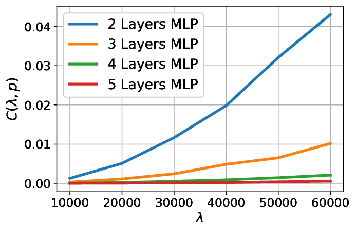
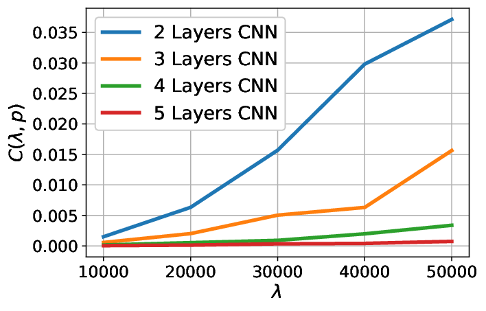
We note that the linear model has the largest expected gradient-norm. Further, note that the deeper the network, the smaller its gradient-norm. As a result, deeper nets can use larger values of $\lambda$ for the generalization bound. Thus, we present our complexity bound as a function of $\lambda$ in Fig. 2(a) and Fig. 2(b). Note, the complexity term $C(\lambda,p)$ reaches its minimum around $\lambda=m$ . Fig. 2(c) studies the effect of a network’s depth on the complexity term. We observe that, as expected based on the earlier plots, deeper networks have a lower complexity term. We attribute this phenomenon to vanishing gradients which create a contractivity property that stabilizes the loss function, i.e., reduces its variability. However, this comes at the expense of expressivity of the deep net, since deep nets with vanishing gradients cannot fit the training data in the learning phase.

Table 1: Comparison of the full PAC-Bayesian generalization bound versus Alquier et al. 2016, Germain et al. 2016, and Dziugaite and Roy 2017. For MNIST we use a three layer fully connected model, while for CIFAR-10 we use a CNN with three convolutional layers. In all settings we used

\lambda=m

and

\sigma_{p}^{2}=0.01

Dataset	Alquier	Germain	Dziugaite	Ours
MNIST	3.36 $\pm$ 5e-4	1.86 $\pm$ 4e-3	0.41 $\pm$ 3e-4	0.04 $\pm$ 5E-4
CIFAR-10	4.81 $\pm$ 1e-2	8.37 $\pm$ 9e-2	-	0.05 $\pm$ 4E-3

Comparison to prior PAC-Bayesian bounds: We compare the proposed bound to Alquier et al. 2016 (bounded version), Germain et al. 2016, and Dziugaite and Roy 2017 on both MNIST and CIFAR. Unlike our bound which assumes the expected loss to be bounded, both Alquier et al. 2016 and Germain et al. 2016 assume the loss to be uniformly bounded by a constant $B$ . Hence, for a fair comparison we estimated $B$ to be the maximum and average loss over the training set and use it to bound the maximum and expected loss respectively. Results are summarized in Tab. 1. Notice, our bound produces tighter generalization bounds compared to the baselines methods for both datasets.

5 Related work

Generalization bounds for deep nets were explored in various settings. VC-theory provides both upper bounds and lower bounds to the network’s VC-dimension, which are linear in the number of network parameters (Bartlett et al. 2017b; Bartlett et al. 2019). While VC theory asserts that such a model should overfit as it can learn any random labeling (e.g., (Zhang et al. 2016)), surprisingly, deep nets generally do not overfit.

Rademacher complexity allows to apply data-dependent bounds to deep nets (Bartlett and Mendelson 2002; Neyshabur et al. 2015; Bartlett et al. 2017a; Golowich et al. 2017; Neyshabur et al. 2018). These bounds rely on the loss and the Lipschitz constant of the network and consequently depend on a product of norms of weight matrices, which scales exponentially in the network depth. Wei and Ma 2019 developed a bound over the gradient-norm of training examples. In contrast, our bound depends on average quantities of the gradient-norm. Thus we answer an open question of Bartlett et al. 2017a about the existence of bounds that depend on average loss and average gradient-norm, albeit in a PAC-Bayesian setting. PAC-Bayesian bounds that use Rademacher complexity have also been studied (Kakade et al. 2009; Yang et al. 2019).

Stability bounds may be applied to unbounded loss functions and in particular to the negative log-likelihood (NLL) loss (Bousquet and Elisseeff 2002; Rakhlin et al. 2005; Shalev-Shwartz et al. 2009; Hardt et al. 2015; Zhang et al. 2016). However, stability bounds for convex loss functions, e.g., for logistic regression, do not apply to deep nets since they require the NLL loss to be a convex function of the parameters. Alternatively, Hardt et al. 2015 and Kuzborskij and Lampert 2017 estimate the stability of stochastic gradient descent dynamics, which strongly relies on early stopping. This approach results in weaker bounds for the non-convex setting. Stability PAC-Bayesian bounds for bounded and Lipschitz loss functions were developed by London 2017. Li et al. 2019 utilized the log-Sobolev inequality to bound the KL divergence under the PAC-Bayesian setting while assuming a bounded loss function. In contrast, we assume an unbounded loss function and a Gaussian prior distribution over the model weights. The latter allows us to compute the KL divergence. Holland 2019 studies PAC-Bayesian learning guarantees for heavy-tailed losses. Haddouche et al. 2021 relax the boundness assumption by modifying the range of the loss to depend on each predictor. Differently, through the log-Sobolev inequality, our bound relies on the expected gradient-norm of the loss function, which may be unbounded as well.

PAC-Bayesian bounds were recently applied to deep nets (McAllester 2013; Dziugaite and Roy 2017; Neyshabur et al. 2017; Pérez-Ortiz et al. 2021). In contrast to our work, those related works all consider bounded loss functions. An excellent survey on PAC-Bayesian bounds was provided by Germain et al. 2016. Alquier et al. 2016 introduced PAC-Bayesian bounds for linear classifiers trained with a hinge-loss by explicitly bounding its moment generating function. Dziugaite et al. 2021 investigate the role of data in learning a PAC-Bayesian prior. Closely, Foong et al. 2021 study the tightness of PAC-Bayesian bounds for small datasets. Alquier et al. 2012 provide an analysis for PAC-Bayesian bounds with Lipschitz functions. Our work differs as we derive PAC-Bayesian bounds for non-Lipschitz functions. Work by Germain et al. 2016 is closer to our setting and considers PAC-Bayesian bounds for linear models and quadratic loss functions. In contrast, our work considers the multi-class setting and non-linear models. PAC-Bayesian bounds for the NLL loss in the online setting were put forward too (Takimoto and Warmuth 2000; Banerjee 2006; Bartlett et al. 2013; Grünwald and Mehta 2017). The online setting does not consider the whole sample space and therefore is simpler to analyze in the Bayesian setting. Recently, a PAC-Bayesian generalization bound for meta-learning was proposed (Rothfuss et al. 2020; Amit and Meir 2018; Farid and Majumdar 2021; Ding et al. 2021). In contrast to our work, Amit and Meir 2018 and Farid and Majumdar 2021 focus on bounded loss functions while Rothfuss et al. 2020 assume the loss function to be sub-gamma.

PAC-Bayesian bounds for the NLL loss function are intimately related to learning Bayesian inference Germain et al. 2016. Recently, many works applied various posteriors in Bayesian deep nets. Gal and Ghahramani 2015; Gal 2016 introduce a Bayesian inference approximation using Monte Carlo (MC) dropout, which approximates a Gaussian posterior using Bernoulli dropout. Srivastava et al. 2014; Kingma et al. 2015 introduced Gaussian dropout, which effectively created a Gaussian posterior that couples the mean and the variance of the learned parameters and explored the relevant log-uniform priors. Blundell et al. 2015; Louizos and Welling 2016 suggest taking a complete Bayesian perspective and learning the mean and the variance of each parameter separately.

Stochastic gradient Langevin dynamics (SGLD) bounds (Pensia et al. 2018; Mou et al. 2018; Negrea et al. 2019; Haghifam et al. 2020) suggest bounding the generalization gap by investigating the dynamics of the parameters through Langevin dynamics and Fokker-Planck equations. Broadly, the Fokker-Planck equation defines a Markov process, and these works measure the KL-divergence between a prior and posterior distribution of this process in the parameter space using gradient norms of the parameters. Differently, our work utilizes the Herbst theorem to measure the KL-divergence (in the form of functional entropy) between prior and posterior in the input space. This distinction leads to a computation of the gradients with respect to different quantities, i.e., parameters vs. input data

6 Discussion and future work

In this study, we present new PAC-Bayesian generalization bounds that depend on the gradient-norm of the loss function. We explore their properties in our experimental validation in various deep learning settings, reinforcing the importance of gradients in contemporary deep nets. Our framework allows for new PAC-Bayesian bounds that assume on-average bounded loss and an on-average bounded gradient norm assumptions. These findings answer an open problem raised by Bartlett et al. 2017a under the PAC-Bayesian setting. Moreover, we extend the current generalization bounds proposed for the hinge-loss to any linear model with a Lipschitz loss function. Finally, we empirically show that our bounds produce tighter generalization performance than the baseline methods. These results are another step towards bridging the gap between theory and practice while having more realistic assumptions for modern deep nets.

Our framework can be extended in different directions. Log-Sobolev inequalities (LSIs) are intimately related to hypercontractivity. Our generalization bounds also imply that deep nets hyper-contracts their input and therefore generalize. While the relation between generalization and hypercontractivity is under explored, with the small-ball theorem as a notable exception (Lecué and Mendelson 2017; Mendelson 2014), we believe it is a fundamental concept in contemporary deep nets that require further research. Additionally, our framework focuses on bounding the complexity term. It is interesting future work to also consider the KL term.

We assume that the labels are balanced with respect to the loss, or equivalently, the influence of all labels is equal. The theory of influence of discrete functions is well-developed and very relevant to LSIs, hypercontractivity, and measure concentration, and further investigation on its relation to generalization is desired (O’Donnell 2014).

References

Zhang et al. [2016] Chiyuan Zhang, Samy Bengio, Moritz Hardt, Benjamin Recht, and Oriol Vinyals. Understanding deep learning requires rethinking generalization. arXiv preprint arXiv:1611.03530, 2016.
Alquier et al. [2016] Pierre Alquier, James Ridgway, and Nicolas Chopin. On the properties of variational approximations of gibbs posteriors. JMLR, 2016.
Alquier et al. [2019] Pierre Alquier, Vincent Cottet, and Guillaume Lecué. Estimation bounds and sharp oracle inequalities of regularized procedures with lipschitz loss functions. The Annals of Statistics, 2019.
Bégin et al. [2016] Luc Bégin, Pascal Germain, François Laviolette, and Jean-Francis Roy. Pac-bayesian bounds based on the rényi divergence. In Artificial Intelligence and Statistics. PMLR, 2016.
Alquier and Guedj [2018] Pierre Alquier and Benjamin Guedj. Simpler pac-bayesian bounds for hostile data. Machine Learning, 2018.
Germain et al. [2016] Pascal Germain, Francis Bach, Alexandre Lacoste, and Simon Lacoste-Julien. Pac-bayesian theory meets bayesian inference. In NeurIPS, 2016.
Haddouche et al. [2021] Maxime Haddouche, Benjamin Guedj, Omar Rivasplata, and John Shawe-Taylor. Pac-bayes unleashed: generalisation bounds with unbounded losses. Entropy, 2021.
van Handel [2016] Ramon van Handel. Probability in high dimension, December 2016.
Bartlett et al. [2017a] Peter L Bartlett, Dylan J Foster, and Matus J Telgarsky. Spectrally-normalized margin bounds for neural networks. In NeurIPS, 2017a.
Gross [1975] Leonard Gross. Logarithmic sobolev inequalities. American Journal of Mathematics, 1975.
Titterington et al. [1985] D.M. Titterington, P.S.D.M. Titterington, S.A.F. M, A.F.M. Smith, U.E. Makov, and John Wiley & Sons. Statistical Analysis of Finite Mixture Distributions. Wiley, 1985.
Scott [1992] David W Scott. Multivariate density estimation: theory, practice, and visualization. John Wiley & Sons, 1992.
Goodfellow et al. [2016] Ian Goodfellow, Yoshua Bengio, and Aaron Courville. Deep learning. MIT press, 2016.
Virmaux and Scaman [2018] Aladin Virmaux and Kevin Scaman. Lipschitz regularity of deep neural networks: analysis and efficient estimation. In NeurIPS, 2018.
Combettes and Pesquet [2019] Patrick L Combettes and Jean-Christophe Pesquet. Lipschitz certificates for neural network structures driven by averaged activation operators. arXiv preprint arXiv:1903.01014, 2019.
Krizhevsky [2009] Alex Krizhevsky. Learning multiple layers of features from tiny images. Technical report, 2009.
Simonyan and Zisserman [2014] Karen Simonyan and Andrew Zisserman. Very deep convolutional networks for large-scale image recognition. arXiv preprint arXiv:1409.1556, 2014.
Szegedy et al. [2015] Christian Szegedy, Wei Liu, Yangqing Jia, Pierre Sermanet, Scott Reed, Dragomir Anguelov, Dumitru Erhan, Vincent Vanhoucke, and Andrew Rabinovich. Going deeper with convolutions. In CVPR, 2015.
He et al. [2016] Kaiming He, Xiangyu Zhang, Shaoqing Ren, and Jian Sun. Deep residual learning for image recognition. In CVPR, 2016.
Huang et al. [2017] Gao Huang, Zhuang Liu, Laurens Van Der Maaten, and Kilian Q Weinberger. Densely connected convolutional networks. In CVPR, 2017.
Howard et al. [2017] Andrew G Howard, Menglong Zhu, Bo Chen, Dmitry Kalenichenko, Weijun Wang, Tobias Weyand, Marco Andreetto, and Hartwig Adam. Mobilenets: Efficient convolutional neural networks for mobile vision applications. arXiv preprint arXiv:1704.04861, 2017.
Tan and Le [2019] Mingxing Tan and Quoc Le. Efficientnet: Rethinking model scaling for convolutional neural networks. In ICML, 2019.
LeCun et al. [1998] Yann LeCun, Léon Bottou, Yoshua Bengio, and Patrick Haffner. Gradient-based learning applied to document recognition. 1998.
Dziugaite and Roy [2017] Gintare Karolina Dziugaite and Daniel M Roy. Computing nonvacuous generalization bounds for deep (stochastic) neural networks with many more parameters than training data. arXiv preprint arXiv:1703.11008, 2017.
Bartlett et al. [2017b] Peter L Bartlett, Nick Harvey, Chris Liaw, and Abbas Mehrabian. Nearly-tight vc-dimension and pseudodimension bounds for piecewise linear neural networks. arXiv preprint arXiv:1703.02930, 2017b.
Bartlett et al. [2019] Peter L. Bartlett, Nick Harvey, Christopher Liaw, and Abbas Mehrabian. Nearly-tight vc-dimension and pseudodimension bounds for piecewise linear neural networks. JMLR, 2019.
Bartlett and Mendelson [2002] Peter L Bartlett and Shahar Mendelson. Rademacher and gaussian complexities: Risk bounds and structural results. JMLR, 2002.
Neyshabur et al. [2015] Behnam Neyshabur, Ryota Tomioka, and Nathan Srebro. Norm-based capacity control in neural networks. In Conference on Learning Theory, pages 1376–1401, 2015.
Golowich et al. [2017] Noah Golowich, Alexander Rakhlin, and Ohad Shamir. Size-independent sample complexity of neural networks. arXiv preprint arXiv:1712.06541, 2017.
Neyshabur et al. [2018] Behnam Neyshabur, Zhiyuan Li, Srinadh Bhojanapalli, Yann LeCun, and Nathan Srebro. Towards understanding the role of over-parametrization in generalization of neural networks. arXiv preprint arXiv:1805.12076, 2018.
Wei and Ma [2019] Colin Wei and Tengyu Ma. Data-dependent sample complexity of deep neural networks via lipschitz augmentation. In NeurIPS, 2019.
Kakade et al. [2009] Sham M Kakade, Karthik Sridharan, and Ambuj Tewari. On the complexity of linear prediction: Risk bounds, margin bounds, and regularization. In NeurIPS, 2009.
Yang et al. [2019] Jun Yang, Shengyang Sun, and Daniel M Roy. Fast-rate pac-bayes generalization bounds via shifted rademacher processes. In NeurIPS, 2019.
Bousquet and Elisseeff [2002] Olivier Bousquet and André Elisseeff. Stability and generalization. JMLR, 2002.
Rakhlin et al. [2005] Alexander Rakhlin, Sayan Mukherjee, and Tomaso Poggio. Stability results in learning theory. Analysis and Applications, 2005.
Shalev-Shwartz et al. [2009] Shai Shalev-Shwartz, Ohad Shamir, Nathan Srebro, and Karthik Sridharan. Stochastic convex optimization. In COLT, 2009.
Hardt et al. [2015] Moritz Hardt, Benjamin Recht, and Yoram Singer. Train faster, generalize better: Stability of stochastic gradient descent. arXiv preprint arXiv:1509.01240, 2015.
Kuzborskij and Lampert [2017] Ilja Kuzborskij and Christoph H Lampert. Data-dependent stability of stochastic gradient descent. arXiv preprint arXiv:1703.01678, 2017.
London [2017] Ben London. A pac-bayesian analysis of randomized learning with application to stochastic gradient descent. In NeurIPS, 2017.
Li et al. [2019] Jian Li, Xuanyuan Luo, and Mingda Qiao. On generalization error bounds of noisy gradient methods for non-convex learning. arXiv preprint arXiv:1902.00621, 2019.
Holland [2019] Matthew Holland. Pac-bayes under potentially heavy tails. NeurIPS, 2019.
McAllester [2013] David McAllester. A pac-bayesian tutorial with a dropout bound. arXiv preprint arXiv:1307.2118, 2013.
Neyshabur et al. [2017] Behnam Neyshabur, Srinadh Bhojanapalli, David McAllester, and Nathan Srebro. A pac-bayesian approach to spectrally-normalized margin bounds for neural networks. arXiv preprint arXiv:1707.09564, 2017.
Pérez-Ortiz et al. [2021] Marıa Pérez-Ortiz, Omar Rivasplata, John Shawe-Taylor, and Csaba Szepesvári. Tighter risk certificates for neural networks. JMLR, 2021.
Dziugaite et al. [2021] Gintare Karolina Dziugaite, Kyle Hsu, Waseem Gharbieh, Gabriel Arpino, and Daniel M Roy. On the role of data in pac-bayes bounds. AISTATS, 2021.
Foong et al. [2021] Andrew YK Foong, Wessel P Bruinsma, David R Burt, and Richard E Turner. How tight can pac-bayes be in the small data regime? In NeurIPS, 2021.
Alquier et al. [2012] Pierre Alquier, Olivier Wintenberger, et al. Model selection for weakly dependent time series forecasting. Bernoulli, 2012.
Takimoto and Warmuth [2000] Eiji Takimoto and Manfred K Warmuth. The last-step minimax algorithm. In International Conference on Algorithmic Learning Theory, pages 279–290. Springer, 2000.
Banerjee [2006] Arindam Banerjee. On bayesian bounds. In ICML, 2006.
Bartlett et al. [2013] Peter Bartlett, Peter Grunwald, Peter Harremoës, Fares Hedayati, and Wojciech Kotlowski. Horizon-independent optimal prediction with log-loss in exponential families. arXiv preprint arXiv:1305.4324, 2013.
Grünwald and Mehta [2017] Peter D Grünwald and Nishant A Mehta. A tight excess risk bound via a unified pac-bayesian-rademacher-shtarkov-mdl complexity. arXiv preprint arXiv:1710.07732, 2017.
Rothfuss et al. [2020] Jonas Rothfuss, Vincent Fortuin, and Andreas Krause. Pacoh: Bayes-optimal meta-learning with pac-guarantees. arXiv preprint arXiv:2002.05551, 2020.
Amit and Meir [2018] Ron Amit and Ron Meir. Meta-learning by adjusting priors based on extended pac-bayes theory. ICML, 2018.
Farid and Majumdar [2021] Alec Farid and Anirudha Majumdar. Generalization bounds for meta-learning via pac-bayes and uniform stability. In NeurIPS, 2021.
Ding et al. [2021] Nan Ding, Xi Chen, Tomer Levinboim, Sebastian Goodman, and Radu Soricut. Bridging the gap between practice and pac-bayes theory in few-shot meta-learning. In NeurIPS, 2021.
Gal and Ghahramani [2015] Yarin Gal and Zoubin Ghahramani. Dropout as a bayesian approximation: Representing model uncertainty in deep learning. arXiv preprint arXiv:1506.02142, 2015.
Gal [2016] Yarin Gal. Uncertainty in deep learning. PhD thesis, PhD thesis, University of Cambridge, 2016.
Srivastava et al. [2014] Nitish Srivastava, Geoffrey Hinton, Alex Krizhevsky, Ilya Sutskever, and Ruslan Salakhutdinov. Dropout: A simple way to prevent neural networks from overfitting. JMLR, 2014.
Kingma et al. [2015] Durk P Kingma, Tim Salimans, and Max Welling. Variational dropout and the local reparameterization trick. In NeurIPS, 2015.
Blundell et al. [2015] Charles Blundell, Julien Cornebise, Koray Kavukcuoglu, and Daan Wierstra. Weight uncertainty in neural networks. arXiv preprint arXiv:1505.05424, 2015.
Louizos and Welling [2016] Christos Louizos and Max Welling. Structured and efficient variational deep learning with matrix gaussian posteriors. In ICLR, 2016.
Pensia et al. [2018] Ankit Pensia, Varun Jog, and Po-Ling Loh. Generalization error bounds for noisy, iterative algorithms. In ISIT, 2018.
Mou et al. [2018] Wenlong Mou, Liwei Wang, Xiyu Zhai, and Kai Zheng. Generalization bounds of sgld for non-convex learning: Two theoretical viewpoints. In Conference on Learning Theory, 2018.
Negrea et al. [2019] Jeffrey Negrea, Mahdi Haghifam, Gintare Karolina Dziugaite, Ashish Khisti, and Daniel M Roy. Information-theoretic generalization bounds for sgld via data-dependent estimates. NeurIPS, 2019.
Haghifam et al. [2020] Mahdi Haghifam, Jeffrey Negrea, Ashish Khisti, Daniel M Roy, and Gintare Karolina Dziugaite. Sharpened generalization bounds based on conditional mutual information and an application to noisy, iterative algorithms. NeurIPS, 2020.
Lecué and Mendelson [2017] Guillaume Lecué and Shahar Mendelson. Regularization and the small-ball method ii: complexity dependent error rates. The Journal of Machine Learning Research, 2017.
Mendelson [2014] Shahar Mendelson. Learning without concentration. In Conference on Learning Theory, 2014.
O’Donnell [2014] Ryan O’Donnell. Analysis of boolean functions. Cambridge University Press, 2014.
Boucheron et al. [2013] Stéphane Boucheron, Gábor Lugosi, and Pascal Massart. Concentration Inequalities: A Nonasymptotic Theory of Independence. OUP, 2013.
Zhang et al. [2019] Hongyi Zhang, Yann N Dauphin, and Tengyu Ma. Fixup initialization: Residual learning without normalization. arXiv preprint arXiv:1901.09321, 2019.
Santurkar et al. [2018] Shibani Santurkar, Dimitris Tsipras, Andrew Ilyas, and Aleksander Madry. How does batch normalization help optimization? In NeurIPS, 2018.

Checklist

1.
For all authors…
1. (a)
  
  Do the main claims made in the abstract and introduction accurately reflect the paper’s contributions and scope? [Yes]
2. (b)
  
  Did you describe the limitations of your work? [Yes]
3. (c)
  
  Did you discuss any potential negative societal impacts of your work? [N/A]
4. (d)
  
  Have you read the ethics review guidelines and ensured that your paper conforms to them? [Yes]
2.
If you are including theoretical results…
1. (a)
  
  Did you state the full set of assumptions of all theoretical results? [Yes]
2. (b)
  
  Did you include complete proofs of all theoretical results? [Yes]
3.
If you ran experiments…
1. (a)
  
  Did you include the code, data, and instructions needed to reproduce the main experimental results (either in the supplemental material or as a URL)? [Yes]
2. (b)
  
  Did you specify all the training details (e.g., data splits, hyperparameters, how they were chosen)? [Yes]
3. (c)
  
  Did you report error bars (e.g., with respect to the random seed after running experiments multiple times)? [Yes]
4. (d)
  
  Did you include the total amount of compute and the type of resources used (e.g., type of GPUs, internal cluster, or cloud provider)? [Yes]
4.
If you are using existing assets (e.g., code, data, models) or curating/releasing new assets…
1. (a)
  
  If your work uses existing assets, did you cite the creators? [Yes]
2. (b)
  
  Did you mention the license of the assets? [N/A]
3. (c)
  
  Did you include any new assets either in the supplemental material or as a URL? [N/A]
4. (d)
  
  Did you discuss whether and how consent was obtained from people whose data you’re using/curating? [N/A]
5. (e)
  
  Did you discuss whether the data you are using/curating contains personally identifiable information or offensive content? [N/A]
5.
If you used crowdsourcing or conducted research with human subjects…
1. (a)
  
  Did you include the full text of instructions given to participants and screenshots, if applicable? [N/A]
2. (b)
  
  Did you describe any potential participant risks, with links to Institutional Review Board (IRB) approvals, if applicable? [N/A]
3. (c)
  
  Did you include the estimated hourly wage paid to participants and the total amount spent on participant compensation? [N/A]

Appendix A Log-Sobolev inequalities

For completeness we derive Theorem 2.3. We begin with proving the LSI for a Rademacher random variable, i.e., a discrete random variable that takes the values $\{-1,+1\}$ with equal probability.

Theorem A.1 (LSI for Rademacher distribution, Gross 1975).

let $Z$ be Rademacher random variable that take values in $\{-1,+1\}$ with probability of $\frac{1}{2}$ . Set the discrete gradient of a function $f:\{-1,+1\}\rightarrow\R$ to be

\displaystyle\nabla f(z)\triangleq\frac{f(z)-f(-z)}{2}.

(27)

Then the following LSI holds:

\displaystyle\ent\left[e^{f(Z)}\right]\leq 2\E_{Z\sim\{-1,+1\}}\left[\left(\nabla e^{f(Z)/2}\right)^{2}\right]=\frac{1}{2}\E_{Z\sim\{-1,+1\}}\left[\left(\nabla f(Z)\right)^{2}e^{f(Z)}\right].

(28)

Proof.

The quantities that constitute the LSI for Rademacher random variables take the form:

	$\displaystyle\ent\left[e^{f(Z)}\right]$	$\displaystyle=$	$\displaystyle\frac{e^{f(1)}f(1)+e^{f(-1)}f(-1)}{2}-\frac{e^{f(1)}+e^{f(-1)}}{2}\log\left(\frac{e^{f(1)}+e^{f(-1)}}{2}\right)$
	$\displaystyle\E_{Z\sim\{-1,+1\}}\left[\left(\nabla e^{f(Z)/2}\right)^{2}\right]$	$\displaystyle=$	$\displaystyle\left(\frac{e^{f(1)/2}-e^{f(-1)/2}}{2}\right)^{2}.$		(29)

Setting $a=f(1)$ and $b=f(-1)$ the log-Sobolev inequality implies that:

\displaystyle\frac{1}{2}(a^{2}\log a^{2}+b^{2}\log b^{2})-\frac{a^{2}+b^{2}}{2}\log\frac{a^{2}+b^{2}}{2}\leq\frac{1}{2}(b-a)^{2}.

(30)

In the following, we assume without loss of generality that $a\leq b$ . Let’s also define

\displaystyle g(r)\triangleq\frac{1}{2}(a^{2}\log a^{2}+r^{2}\log r^{2})-\frac{a^{2}+r^{2}}{2}\log\frac{a^{2}+r^{2}}{2}-\frac{1}{2}(r-a)^{2}.

(31)

Given this notation, proving the LSI for Rademancher random variables amounts to proving that $g(b)\leq 0$ . To prove the inequality $g(b)\leq 0$ we follow these steps:

1.

$g^{\prime}(a)=0$ ,
2.

for any $a<r\leq b$ holds $g^{\prime}(r)\leq 0$ .

First, we have:

	$\displaystyle g^{\prime}(r)$	$\displaystyle=$	$\displaystyle r\log r^{2}+r-r\left(\log\left(\frac{a^{2}+r^{2}}{2}\right)+1\right)-(r-a)$		(32)
		$\displaystyle=$	$\displaystyle r\log r^{2}-r\log\left(\frac{a^{2}+r^{2}}{2}\right)-(r-a).$		(33)

One can easily verify that $g^{\prime}(a)=0$ . To prove that $g^{\prime}(r)\leq 0$ we show that $g^{\prime\prime}(r)\leq 0$ for any $a<r\leq b$ , thus guaranteeing that $g^{\prime}(r)$ is non-positive.

	$\displaystyle g^{\prime\prime}(r)$	$\displaystyle=$	$\displaystyle\log r^{2}+2-\log\left(\frac{a^{2}+r^{2}}{2}\right)-\frac{2r^{2}}{a^{2}+r^{2}}-1$		(34)
		$\displaystyle=$	$\displaystyle\log\left(\frac{2r^{2}}{a^{2}+r^{2}}\right)-\frac{2r^{2}}{a^{2}+r^{2}}+1.$		(35)

Using the fact that $1+\log\alpha-\alpha\leq 0$ for any $\alpha$ we are able to verify that $g^{\prime\prime}(r)\leq 0$ . ∎

The LSI for Rademacher complexity extends to Gaussian distributions using the central limit theorem, which asserts that an average of i.i.d. Rademacher random variables converges to Gaussian distribution. This extension relies on tensorization of the functional entropy, which effortlessly scales to high-dimensional settings.

Theorem A.2 (Tensorization of Rademacher random variables, Gross 1975, Boucheron et al. 2013).

Let $Z_{1},...,Z_{d}$ be i.i.d. Rademacher random variables and let

$\displaystyle\ent_{i}[f(z_{1},...,z_{d})]$	$\displaystyle\triangleq$	$\displaystyle\ent[f(z_{1},...,z_{i-1},Z_{i},z_{i+1},...,z_{d})]$	(36)
	$\displaystyle\triangleq$	$\displaystyle\E_{Z_{i}}[f(z_{1},...,z_{i-1},Z_{i},z_{i+1},...,z_{d})\log(f(z_{1},...,z_{i-1},Z_{i},z_{i+1},...,z_{d}))]$	(37)
		$\displaystyle-\left(\E_{Z_{i}}[f(z_{1},...,z_{i-1},Z_{i},z_{i+1},...,z_{d})]\right)\log\left(\E_{Z_{i}}[f(z_{1},...,z_{i-1},Z_{i},z_{i+1},...,z_{d})]\right).$	(37)

Tensorization of independent random variables $Z_{1},...,Z_{d}$ implies the bound:

\ent[f(Z_{1},...,Z_{d})]\leq\E_{Z_{1},...,Z_{d}}[\sum_{i=1}^{d}\ent_{i}[f(Z_{1},...,Z_{d})]].

(38)

Proof.

We denote the $d$ -th tuple by $z=(z_{1},...,z_{d})$ and set $z_{[d]\setminus i}=(z_{1},...,z_{i-1},z_{i+1},...,z_{d})$ . Following the definitions:

	$\displaystyle\ent[f(Z_{1},...,Z_{d})]$	$\displaystyle=$	$\displaystyle 2^{-d}\sum_{z}f(z)\log f(z)-\left(2^{-d}\sum_{z}f(z)\right)\log\left(2^{-d}\sum_{z}f(z)\right),$		(39)
	$\displaystyle\ent_{i}[f(z_{1},...,z_{d})]$	$\displaystyle=$	$\displaystyle 2^{-1}\sum_{z_{i}}f(z)\log(f(z))-\left(2^{-1}\sum_{z_{i}}f(z)\right)\log\left(2^{-1}\sum_{z_{i}}f(z)\right).$		(40)

We assume without loss of generality²² 2 Since $\ent(cf)=c\ent(f)$ , for any $c>0$ , then $\ent[cf]\leq\E[\sum_{i=1}^{d}\ent_{i}[cf]]$ if and only if $\ent[f]\leq\E[\sum_{i=1}^{d}\ent_{i}[f]]$ . that $\sum_{z}2^{-d}f(z)=1$ and set $q(z)\triangleq 2^{-d}f(z)$ . Since $f(z)\geq 0$ , then $q(z)$ is a distribution and its entropy is $H(q)=-\sum_{z}q(z)\log q(z)$ . Then:

\displaystyle\ent[f(Z_{1},...,Z_{d})]

\displaystyle=

\displaystyle d-H(q).

(42)

We denote the marginal distribution by $q(z_{[d]\setminus i})=\sum_{z_{i}}q(z_{[d]\setminus i},z_{i})$ . Then

	$\displaystyle\ent_{i}[f(z_{1},...,z_{d})]$	$\displaystyle=$	$\displaystyle\sum_{z_{i}}q(z_{[d]\setminus i},z_{i})\log(q(z_{[d]\setminus i},z_{i}))-q(z_{[d]\setminus i})\log(q(z_{[d]\setminus i})),$		(43)
	$\displaystyle\E_{Z_{1},...,Z_{d}}[\ent_{i}[f(z_{1},...,z_{d})]]$	$\displaystyle=$	$\displaystyle-H(q)+H(q_{[d]\setminus i})+1,$		(44)

where $q_{[d]\setminus i}$ is the distribution of $q(z_{[d]\setminus i})$ . With these equalities in mind,

\displaystyle\ent[f(Z_{1},...,Z_{d})]\leq\E_{Z_{1},...,Z_{d}}\left[\sum_{i=1}^{d}\ent_{i}[f(z_{1},...,z_{d})]\right]\Longleftrightarrow H(q)\leq\frac{1}{d-1}\sum_{i=1}^{d}H(q_{[d]\setminus i})\;\;\;\mbox{(Han's inequality)}.

(45)

The right hand side of the above equation is know as Han’s inequality.

∎

We use tensorization and the central limit theorem to extend the LSI of Rademacher random variables to derive the LSI for Gaussian random variables.

Theorem A.3 (Gaussian log-Sobolev inequality (LSI), Gross 1975).

Let $Z$ be a Gaussian random variables $Z\sim{\cal N}(0,1)$ . Then

\ent[e^{f(Z)}]\leq\frac{1}{2}\E[f^{\prime}(Z)^{2}e^{f(Z)}].

(46)

Proof.

In the following we denote by $Z_{1},...,Z_{d}$ Rademacher random variables. We set $f_{d}(Z_{1},...,Z_{d})=f\left(\frac{\sum_{i=1}^{d}Z_{i}}{\sqrt{d}}\right)$ . Using tensorization and the LSI for Rademacher random variables:

$\displaystyle\ent[f_{d}(Z_{1},...,Z_{d})]$	$\displaystyle\leq$	$\displaystyle\E_{Z_{1},...,Z_{d}}[\sum_{i=1}^{d}\ent_{i}[f_{d}(Z_{1},...,Z_{d})]]$	(47)
	$\displaystyle\hskip-113.81102pt\leq$	$\displaystyle\hskip-56.9055pt\frac{1}{2}\E_{Z_{1},...,Z_{d}}\left[\sum_{i=1}^{d}\E_{Z_{i}\sim\{-1,+1\}}\left[\left(\frac{f\left(\frac{\sum_{j=1}^{d}Z_{j}}{\sqrt{d}}\right)-f\left(\frac{\sum_{j\neq i}^{d}Z_{j}}{\sqrt{d}}-\frac{Z_{i}}{\sqrt{d}}\right)}{2}\right)^{2}e^{f\left(\frac{\sum_{i=1}^{d}Z_{i}}{\sqrt{d}}\right)}\right]\right]$	(48)
	$\displaystyle\hskip-113.81102pt=$	$\displaystyle\hskip-56.9055pt\frac{1}{2}\E_{Z_{1},...,Z_{d}}\left[\frac{1}{d}\sum_{i=1}^{d}\E_{Z_{i}\sim\{-1,+1\}}\left[\left(\frac{f\left(\frac{\sum_{j=1}^{d}Z_{j}}{\sqrt{d}}\right)-f\left(\frac{\sum_{j\neq i}^{d}Z_{j}}{\sqrt{d}}-\frac{Z_{i}}{\sqrt{d}}\right)}{\frac{2}{\sqrt{d}}}\right)^{2}e^{f\left(\frac{\sum_{i=1}^{d}Z_{i}}{\sqrt{d}}\right)}\right]\right].$	(49)

The theorem follows using the central limit theorem as $\lim_{d\rightarrow\infty}\frac{\sum_{i=1}^{d}Z_{i}}{\sqrt{d}}=Z$ , when $Z\sim{\cal N}(0,1)$ and

	$\displaystyle f(Z)$	$\displaystyle=$	$\displaystyle\lim_{d\rightarrow\infty}f_{d}(Z_{1},...,Z_{d}),$		(50)
	$\displaystyle f^{\prime}(Z)$	$\displaystyle=$	$\displaystyle\lim_{d\rightarrow\infty}\frac{f\left(\frac{\sum_{j=1}^{d}Z_{j}}{\sqrt{d}}\right)-f\left(\frac{\sum_{j\neq i}^{d}Z_{j}}{\sqrt{d}}-\frac{Z_{i}}{\sqrt{d}}\right)}{\frac{2}{\sqrt{d}}}.$		(51)

∎

The above provides a LSI for the standard Gaussian distribution. While we can use the same technique to prove a LSI for $Z\sim{\cal N}(\mu,\sigma^{2})$ , we separate these two theorems for clarity and turn to prove the general case as a corollary.

Theorem A.4 (Gaussian log-Sobolev inequality (LSI), Gross 1975).

Let $Z\sim{\cal N}(\mu,\sigma^{2})$ be a Gaussian random variable with mean $\mu$ and variance $\sigma^{2}$ . Then

\ent[e^{f(Z)}]\leq\frac{1}{2}\sigma^{2}\E[f^{\prime}(Z)^{2}e^{f(Z)}].

(52)

Proof.

The proof follows via a simple change of variable. Let $\hat{Z}\sim{\cal N}(0,1)$ , then $\mu+\sigma\hat{Z}\sim{\cal N}(\mu,\sigma^{2})$ . We set $g(\hat{Z})\triangleq f(\mu+\sigma Z)$ . We use the LSI for the standard Gaussian: $\ent[e^{g(\hat{Z})}]\leq\frac{1}{2}\E[g^{\prime}(\hat{Z})^{2}e^{g(\hat{Z})}]$ and note that $g^{\prime}(\hat{z})=\sigma f^{\prime}(z)$ . ∎

Theorem 2.3 for multivariate Gaussians holds when applying tensorization for each Gaussian independently.

Appendix B Proofs

Theorem B.1.

\displaystyle\E_{w\sim q}[L_{D}(w)]\leq\E_{w\sim q}[L_{S}(w)]+\frac{kd\log(\sqrt{4/3})+KL(q||p)+\log(1/\delta)}{\lambda}.

(53)

Proof.

	$\displaystyle\E_{\D}\Big[\\|\sigma_{y}\nabla\ell(w,x,y)\\|^{2}\int_{0}^{\frac{\lambda}{m}}\frac{e^{-\alpha\ell(w,x,y)}}{M(\alpha)}d\alpha\Big]$	$\displaystyle\leq$	$\displaystyle\sigma_{y}^{2}g^{2}\sum_{y=1}^{k}\sum_{j=1}^{d}w_{y,j}^{2}\cdot\E_{\D}\Big[\int_{0}^{\frac{\lambda}{m}}\frac{e^{-\alpha\ell(w,x,y)}}{M(\alpha)}d\alpha\Big]$
		$\displaystyle=$	$\displaystyle\sigma_{y}^{2}g^{2}\sum_{y=1}^{k}\sum_{j=1}^{d}w_{y,j}^{2}\int_{0}^{\frac{\lambda}{m}}\frac{\E_{\D}\big[e^{-\alpha\ell(w,x,y)}\big]}{M(\alpha)}d\alpha.$

\displaystyle C(\lambda,p)

\displaystyle\leq

\displaystyle\log\Big(\E_{w\sim p}e^{\frac{\sigma_{y}^{2}\lambda^{2}g^{2}}{2m}\sum_{y,j}w_{y,j}^{2}}\Big).

(54)

Finally, whenever $\lambda g\sigma_{p}\sigma_{y}\leq\sqrt{m/4}$ we follow the Gaussian integral and derive the bound

	$\displaystyle\log\Big(\E_{w\sim p}e^{\frac{\sigma_{y}^{2}\lambda^{2}g^{2}}{2m}\sum_{y,j}w_{y,j}^{2}}\Big)$	$\displaystyle=$	$\displaystyle\log\Big(\sqrt{\frac{m}{m-4\sigma_{y}^{2}\lambda^{2}g^{2}\sigma_{p}^{2}}}\Big)^{kd}$		(55)
		$\displaystyle\leq$	$\displaystyle kd\cdot\log\Big(\sqrt{\frac{m}{m-m/4}}\Big)=kd\cdot\log(\sqrt{4/3}).$		(56)

Finally, we obtain Equation (53) by plugging the above into Theorem 2.1. ∎

Theorem B.2.

\displaystyle\E_{w\sim q}[L_{D}(w)]\leq\E_{w\sim q}[L_{S}(w)]+\frac{\frac{\lambda^{2}e^{b}g\sigma_{y}^{2}}{2m}+KL(q||p)+\log(1/\delta)]}{\lambda}.

(57)

Proof.

\displaystyle e^{-\alpha\ell(x,x,y)}\leq 1.

(58)

Then, we lower bound $M(\alpha)\geq M(1)$ for any $0\leq\alpha\leq\lambda/m$ : we note that $0<\lambda\leq m$ , therefore we consider $0\leq\alpha\leq 1$ . Also, since $\ell(w,x,y)\geq 0$ the function $e^{-\alpha\ell(w,x,y)}$ is monotone in $\alpha$ within the unit interval, i.e., for $0\leq\alpha_{1}\leq\alpha_{2}\leq 1$ there holds

\displaystyle e^{-\alpha_{1}\ell(w,x,y)}\geq e^{-\alpha_{2}\ell(w,x,y)}

(59)

and consequently $M(\alpha)\geq M(1)$ for any $\alpha\leq 1$ . Lastly, the assumption $\E_{\D}[-\ell(w,x,y)]\geq-b$ and the monotonicity of the exponential function result in the lower bound

\displaystyle e^{\E_{\D}[-\ell(w,x,y)]}\geq e^{-b}.

(60)

From convexity of the exponential function, $M(1)=\E_{\D}e^{-\ell(w,x,y)}\geq e^{\E_{\D}[-\ell(w,x,y)]}$ , and the lower bound $M(1)\geq e^{-b}$ follows.

Combining these bounds we derive the upper bound

\displaystyle\int_{0}^{1}\frac{e^{-\alpha\ell(w,x,y)}}{M(\alpha)}d\alpha\leq\int_{0}^{1}\frac{1}{e^{-b}}d\alpha=e^{b},

(61)

and the result follows.

Next, by replacing $\E_{\D}\big[\|\sigma_{y}\nabla\ell(w,x,y)\|^{2}\big]$ with $g\sigma_{y}^{2}$ , we obtain

	$\displaystyle C(\lambda,p)\leq$	$\displaystyle\log\E_{w\sim p}e^{\frac{1}{2}\lambda\E_{\D}\big[\\|\sigma_{y}\nabla\ell(w,x,y)\\|^{2}\int_{0}^{\frac{\lambda}{m}}\frac{e^{-\alpha\ell(w,x,y)}}{M(\alpha)}d\alpha\big]}$		(62)
	$\displaystyle\leq$	$\displaystyle\log\E_{w\sim p}e^{\frac{\lambda^{2}e^{b}g\sigma_{y}^{2}}{2m}}=\frac{\lambda^{2}e^{b}g\sigma_{y}^{2}}{2m}.$		(62)

Finally, we obtain Equation (57) by plugging Equation (62) into Theorem 2.1. ∎

Appendix C Additional results

C.1 Connection between generalization and bound

To further demonstrate the use of the bound, we performed a new experiment. We study the effect of important components in ResNet using our bound. For this, we train four variations of the ResNet18 model: 1) a standard model (ResNet); 2) a model without skip connections (ResNetNoSkip); 3) a model without batch normalization layers (ResNetNoBN); and 4) a model without both skip connections and batch normalization layers (ResNetNoSkipNoBN). We optimize all models on the CIFAR10 data:

Model	Test loss	Train loss	Bound on $C(\sqrt{m},p)$
ResNet	0.722 $\pm$ 0.01	0.541 $\pm$ 0.06	0.185 $\pm$ 0.006
ResNetNoSkip	0.631 $\pm$ 0.02	0.478 $\pm$ 0.05	0.179 $\pm$ 0.009
ResNetNoBN	0.603 $\pm$ 0.05	0.564 $\pm$ 0.08	0.172 $\pm$ 0.007
ResNetNoSkipNoBN	2.302 $\pm$ 0.01	2.31 $\pm$ 0.02	0.01 $\pm$ 0.0004

We observe that ResNet and ResNetNoSkip achieve comparable performance in all metrics. Additionally, removing the batch normalization layers and including the skip connections achieves comparable performance to ResNet and ResNetNoSkip. Similar to Zhang et al. 2019, this finding suggests that even without batch normalization, models can converge using precise initialization. Interestingly, by removing batch normalization and skip connection layers, the model gets to a rate of $\lambda=m$ and achieves a good generalization bound. However, this comes at the expense of poor model fitting to the train set due to gradient vanishing. These results are consistent with prior findings in which batch normalization improves optimization [Santurkar et al. 2018]. To conclude, we were able to obtain a tight upper bound of the generalization gap with our proposed bound. However, it is important to note that when using any generalization bound, one should care about the training loss as well as the complexity term.

C.2 Gradient statistics

We further study the gradient norm statistics, we report the max and mean values of the gradient norm (not squared) using the same networks described in Section. 4 in the main paper:

# layers	MNIST (mean)	MNIST (max)	CIFAR (mean)	CIFAR (max)
1	0.00224	0.00267	0.0258	0.0314
2	0.00088	0.0012	0.011	0.015
3	0.00036	0.00056	0.0049	0.008

We observe that the maximum value of the gradient norm is not higher than twice the mean value.

Appendix D Experimental setup

For all MNIST experiments we use MLPs of depth $d\in\{1,\dots,5\}$ . For CIFAR10 experiments we use CNNs of depth $d\in\{2,\dots,5\}$ . For the CNN models, $d$ denotes the number of convolutional layers. We also added a max-pooling layer after each convolutional layer. We included two additional fully connected layers in all CNN models to fix the target output dimension. In all models, we use the ReLU activation function. We optimize the negative log-likelihood (NLL) loss function using stochastic gradient descent (SGD) with a learning rate of 0.01 and a momentum value of 0.9 in all settings for 50 epochs. We use mini-batches of size 128 and did not use any learning rate scheduler. To span the possible weights, we sampled from a normal prior distribution with different variances. For a fair comparison, we set the layers’ width to reach roughly the same number of parameters in each model (except for the linear case). All reported results use $\delta=0.01$ .