OPERA: Omni-Supervised Representation Learning with Hierarchical Supervisions
Abstract
The pretrain-finetune paradigm in modern computer vision facilitates the success of self-supervised learning, which achieves better transferability than supervised learning. However, with the availability of massive labeled data, a natural question emerges: how to train a better model with both self and full supervision signals? In this paper, we propose Omni-suPErvised Representation leArning with hierarchical supervisions (OPERA) as a solution. We provide a unified perspective of supervisions from labeled and unlabeled data and propose a unified framework of fully supervised and self-supervised learning. We extract a set of hierarchical proxy representations for each image and impose self and full supervisions on the corresponding proxy representations. Extensive experiments on both convolutional neural networks and vision transformers demonstrate the superiority of OPERA in image classification, segmentation, and object detection. Code is available at: https://github.com/wangck20/OPERA.
1 Introduction
Learning good representations is a significant yet challenging task in deep learning chen2021exploring; zheng2021deepr; he2020momentum. Researchers have developed various ways to adapt to different supervisions, such as fully supervised oh2018modeling; kim2020proxy; wang2016joint; verma2019manifold, self-supervised wang2015unsupervised; ye2020probabilistic; grill2020bootstrap; chen2020simple, and semi-supervised learning xu2021end; zhang2021flexmatch; wang2022np. They serve as fundamental procedures in various tasks including image classification deng2019arcface; zhang2018mixup; yun2019cutmix, semantic segmentation grill2020bootstrap; strudel2021segmenter, and object detection he2017mask; yang2019reppoints; carion2020end.

Fully supervised learning (FSL) has always been the default choice for representation learning, which learns from discriminating samples with different ground-truth labels. However, this dominance begins to fade with the rise of the pretrain-finetune paradigm in modern computer vision. Under such a paradigm, researchers usually pretrain a network on a large dataset first and then transfer it to downstream tasks he2021masked; chu2021twins; he2020momentum; chen2021exploring. This advocates transferability more than discriminativeness of the learned representations. This preference nurtures the recent success of self-supervised learning (SSL) methods with contrastive objective he2020momentum; xie2021detco; grill2020bootstrap; chen2020simple; wang2022contrastive. They require two views (augmentations) of the same image to be consistent and distinct from other images in the representation space. This instance-level supervision is said to obtain more general and thus transferable representations ericsson2021well; islam2021broad. The ability to learn without human-annotated labels also greatly popularizes self-supervised contrastive learning. Despite its advantages, we want to explore whether combining self-supervised signals11 1 We mainly focus on self-supervised contrastive learning. In the rest of the paper, we use self-supervised learning to refer to self-supervised contrastive learning unless otherwise specified for simplicity. with fully supervised signals further improves the transferability, given the already availability of massive annotated labels russakovsky2015imagenet; lin2014microsoft; abu2016youtube; caesar2020nuscenes.

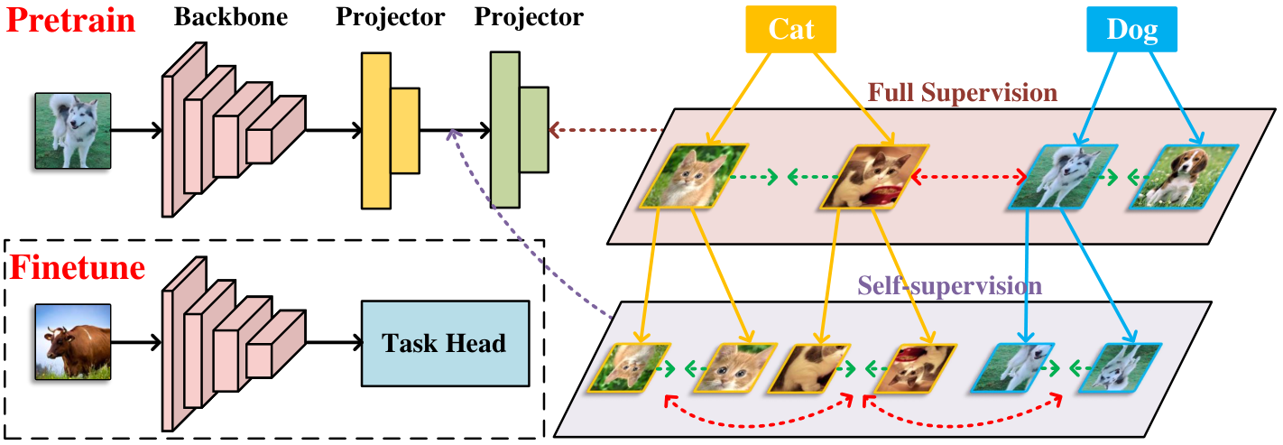
We find that a simple combination of the self and full supervisions results in contradictory training signals. To address this, in this paper, we provide Omni-suPErvised Representation leArning with hierarchical supervisions (OPERA) as a solution, as demonstrated in Figure 2. We unify full and self supervisions in a similarity learning framework where they differ only by the definition of positive and negative pairs. Instead of directly imposing supervisions on the representations, we extract a hierarchy of proxy representations to receive the corresponding supervision signals. Extensive experiments are conducted with both convolutional neural networks he2016deep and vision transformers dosovitskiy2020image as the backbone model. We pretrain the models using OPERA on ImageNet-1K russakovsky2015imagenet and then transfer them to various downstream tasks to evaluate the transferability. We report image classification accuracy with both linear probe and end-to-end finetuning on ImageNet-1K. We also conduct experiments when transferring the pretrained model to other classification tasks, semantic segmentation, and object detection. Experimental results demonstrate consistent improvements over FSL and SSL on all the downstream tasks, as shown in Figure 1. Additionally, we show that OPERA outperforms the counterpart methods even with fewer pretraining epochs (e.g., fewer than 150 epochs), demonstrating good data efficiency.
2 Related Work
Fully Supervised Representation Learning. Fully supervised representation learning (FSL) utilizes the ground-truth labels of data to learn a discriminative representation space. The general objective is to maximize the discrepancies of representations from different categories and minimize those from the same class. The softmax loss is widely used for FSL he2016deep; liu2021swin; deng2019arcface; wang2018cosface, and various loss functions are further developed in deep metric learning kim2020proxy; wang2019multi; hu2014discriminative; movshovitz2017no; teh2020proxynca++.
As fully supervised objectives entail strong constraints, the learned representations are usually more suitable for the specialized classification task and thus lag behind on transferability zhao2020makes; ericsson2021well; islam2021broad. To alleviate this, many works devise various data augmentation methods to expand the training distribution zhang2018mixup; kim2020puzzle; chen2022transmix; venkataramanan2022alignmixup. Recent works also explore adding more layers after the representation to avoid direct supervision vo2019generalization; wang2022revisiting. Differently, we focus on effectively combining self and full supervisions to improve transferability.
Self-supervised Representation Learning. Self-supervised representation learning (SSL) attracts increasing attention in recent years due to its ability to learn meaningful representation without human-annotated labels. The main idea is to train the model to perform a carefully designed label-free pretext task. Early self-supervised learning methods devised various pretext tasks including image restoration vincent2008extracting; zhang2016colorful; pathak2016context, prediction of image rotation gidaris2018unsupervised, and solving jigsaw puzzles noroozi2016unsupervised. They achieve fair performance but still cannot equal fully supervised learning until the arise of self-supervised contrastive learning he2020momentum; chen2020simple; grill2020bootstrap. The pretext task of contrastive learning is instance discrimination, i.e., to identify different views (augmentations) of the same image from those of other images. Contrastive learning methods chen2021exploring; xie2021detco; wang2022cp2; xie2020pointcontrast; liu2020self; chen2021multisiam; hou2021pri3d; liang2021exploring demonstrate even better transferability than fully supervised learning, resulting from their focus on lower-level and thus more general features zhao2020makes; ericsson2021well; islam2021broad. Very recently, masked image modeling (MIM) he2021masked; zhou2021ibot; xie2022simmim emerges as a strong competitor to contrastive learning, which trains the model to correctly predict the masked parts of the input image. In this paper, we mainly focus on contrastive learning in self-supervised learning. Our framework can be extended to other pretext tasks by inserting a new task space in the hierarchy.
Omni-supervised Representation Learning: It is worth mentioning that some existing studies have attempted to combine FSL and SSL radosavovic2018data; nayman2022diverse; wei2022can. Radosavovic et el. radosavovic2018data first trained an FSL model and then performed knowledge distillation on unlabeled data. Wei et el. wei2022can adopted an SSL pretrained model to generate instance labels and compute an overall similarity to train a new model. Nayman et el. nayman2022diverse proposed to finetune an SSL pretrained model using ground-truth labels in a controlled manner to enhance its transferability. Nevertheless, they do not consider the hierarchical relations between the self and full supervision. Also, they perform SSL and FSL sequentially in separate stages. Differently, OPERA unifies them in a universal perspective and imposes the supervisions on different levels of the representations. Our framework can be trained in an end-to-end manner efficiently with fewer epochs.
3 Proposed Approach
In this section, we first present a unified perspective of self-supervised learning (SSL) and fully supervised learning (FSL) under a similarity learning framework. We then propose OPERA to impose hierarchical supervisions on the corresponding hierarchical representations for better transferability. Lastly, we elaborate on the instantiation of the proposed OPERA framework.
3.1 Unified Framework of Similarity Learning
Given an image space , deep representation learning trains a deep neural network as the map to their representation space . Fully supervised learning and self-supervised learning are two mainstream representation learning approaches in modern deep learning. FSL utilizes the human-annotated labels as explicit supervision to train a discriminative classifier. Differently, SSL trains models without ground-truth labels. The widely used contrastive learning (e.g., MoCo-v3 chen2021empirical) obtains meaningful representations by maximizing the similarity between random augmentations of the same image.
Generally, FSL and SSL differ in both the supervision form and optimization objective. To integrate them, we first provide a unified similarity learning framework to include both training objectives:
| (1) | ||||
where and denote the coefficients of positive and negative pairs, and are the labels of the samples, and defines the pairwise similarity between and . is an indicator function which outputs 1 if and 0 otherwise. is the label space, and can be the same as , a transformation of , or a learnable class prototype space. For example, to obtain the softmax objective widely employed in FSL he2016deep; touvron2021training, we can set:
| (2) |
where , and is the row vector in the classifier matrix . For the InfoNCE loss used in contrastive learning van2018representation; he2020momentum; khosla2020supervised, we set:
| (3) | |||
where is the temperature hyper-parameter. See Section A.1 for more details.
Under the unified training objective (1), the main difference between FSL and SSL lies in the definition of the label space and . For the labels in FSL, only if they are from the same ground-truth category. For the labels in SSL, only if they are the augmented views of the same image.
3.2 Hierarchical Supervisions on Hierarchical Representations
With the same formulation of the training objective, a naive way to combine the two training signals is to simply add them:
| (4) | ||||
For and from the same class, i.e., and , the training loss is:
| (5) |
This indicates the two training signals are contradictory and may neutralize each other. This is particularly harmful if we adopt similar loss functions for fully supervised and self-supervised learning, i.e., , and thus .
Existing methods nayman2022diverse; wei2022can; wang2022revisiting address this by subsequently imposing the two training signals. They tend to first obtain a self-supervised pretrained model and then use the full supervision to tune it. Differently, we propose a more efficient way to adaptively balance the two weights so that we can simultaneously employ them:
| (6) |
where and are modulation factors that can be dependent on and for more flexibility. However, it remains challenging to design the specific formulation of and .
Considering that the two label spaces are entangled and demonstrate a hierarchical structure:
| (7) |
i.e., the two augmented views of the same image must share the same category label, we transform the image representation into proxy representations in an instance space and a class space to construct a hierarchical structure. Formally, we apply two transformations sequentially:
| (8) |
where and denote the mapping functions. We extract the class representations following the instance representations since full supervision encodes higher-level features than self-supervision.
We then impose the self and full supervision on the instance space and class space, respectively, to formulate the overall training objective for the proposed OPERA:
| (9) | ||||
We will show in the next subsection that this objective naturally implies (6), which implicitly and adaptively balances self and full supervisions in the representation space.
3.3 Omni-supervised Representation Learning
To effectively combine the self and full supervision to learn representations, OPERA further extracts a set of proxy representations hierarchically to receive the corresponding training signal, as illustrated in Figure 3. Despite its simplicity and efficiency, it is not clear how it achieves balances between the two supervision signals and how it resolves the contradiction demonstrated in (5).
To thoroughly understand the effect of (9) on the image representations, we project it back on the representation space and obtain an equivalent training objective in .
Proposition 1.
Assume using linear projection as the transformation between representation spaces. and , where and are learnable parameters. Optimizing (9) is equivalent to optimizing the following objective on the original representation space :
| (10) | ||||
where and are scalars related to the transformation parameters.
We give detailed proof in Section A.2.
Remark.
Proposition 1 only considers the case without activation functions. We conjecture that the mappings and only influence the form of without altering the final conclusion.
Proposition 1 induces two corollaries as proved in Section A.3 and Section A.4.
Corollary 1.
The loss weight on a pair of samples satisfies:
| (11) | ||||
Corollary 2.
We resolve the contradictory in (5) by adaptively adjusting the loss weight by
| (12) |
Corollary 1 ensures that the learned representations are consistent with how humans perceive the similarities of images, i.e., the similarities between different images of the same class should be larger than those between images of different classes but smaller than those between the views of the same images. Corollary 2 demonstrates the ability of OPERA to adaptively balance the training signals of self and full supervisions.
OPERA can be trained in an end-to-end manner using both self and full supervisions. We extract proxy representations in hierarchical spaces to receive the corresponding training signals. For inference, we discard the proxy representations and directly add the task head on the image representation space .
3.4 Instantiation of OPERA
We present the instantiation of the proposed omni-supervised representation learning with hierarchical supervisions. In the pretraining procedure, we extract hierarchical proxy representations for each image in our model, denoted as . We conduct self-supervised learning with the instance-level label on the instance-level representation and the class-level label is imposed on . The overall objective of our framework follows (9) and OPERA can be optimized in an end-to-end manner. During finetuning, the downstream task head is directly applied to the learned representations . The transfer learning includes image classification and other dense prediction tasks such as semantic segmentation.
In this paper, we apply OPERA to MoCo-v3 chen2021empirical by instantiating as the output of the online predictor and the target predictor denoted as and , respectively. Additionally, is the widely-used InfoNCE loss van2018representation. Furthermore, we employ an extra MLP block that explicitly connects to the online predictor to obtain and fix the output dimension to the class number of the pretrained dataset (e.g., 1,000 for ImageNet). We then introduce full supervision on with the Softmax loss. The overall objective based on MoCo-v3 is as follows:
| (13) | ||||
where denotes the th component of . In addition, we also adopt the stop-gradient operation and the momentum update to the target network following he2020momentum. Therefore, the proposed OPERA framework preserves the instance-level information in MoCo-v3 to prevent damaging the transferability of the model. Furthermore, OPERA involves class-level knowledge with the class-level full supervision, which further boosts the performance of the learned representations.
4 Experiments
In this section, we conducted extensive experiments to evaluate the performance of our OPERA framework. We pretrained the network using OPERA on the ImageNet-1K russakovsky2015imagenet (IN) dataset and then evaluated its performance on different tasks. We provide in-depth ablation studies to analyze the effectiveness of OPERA. All experiments were conducted with PyTorch paszke2019pytorch using RTX 3090 GPUs.
4.1 Experimental Setup
Datasets. We pretrain our model on the training set of ImageNet-1K russakovsky2015imagenet containing 1,200,000 samples of 1,000 categories. We evaluate the linear probe and end-to-end finetuning performance on the validation set consisting of 50,000 images. For transferring to other classification tasks, we use CIFAR-10 krizhevsky2009learning, CIFAR-100 krizhevsky2009learning, Oxford Flowers-102 nilsback2008automated, and Oxford-IIIT-Pets parkhi2012cats. For other downstream tasks, we use ADE20K zhou2019semantic for semantic segmentation and COCO lin2014microsoft for object detection and instance segmentation.
Implementation Details.We mainly applied our OPERA to MoCo-v3 chen2021empirical. We added an extra MLP block after the predictor of the online network, which is composed of two fully-connected layers with a batch normalization layer and a ReLU layer. The hidden dimension of the MLP block was set to while the output dimension was . We trained ResNet50 he2016deep (R50) and ViTs touvron2021training; dosovitskiy2020image (ViT-S and ViT-B) as our backbone with a batch size of , , and . We adopted LARS you2017large as the optimizer for R50 and AdamW loshchilov2018decoupled for ViT. We set the other settings the same as the original MoCo-v3 for fair comparisons. In the following experiments, denotes our reproduced results with the same settings and BS denotes the batch size. P.T and F.T denote the pretraining and finetuning epochs, respectively. The bold number highlights the improvement of OPERA compared with the associated method, and the red number indicates the best performance.
| Method | BS | P.T. | F.T. | Backbone | Top-1 Acc | Top-5 Acc |
|---|---|---|---|---|---|---|
| MoCo-v1 | 256 | 200 | 100 | R50 | 60.6 | - |
| MoCo-v2 | 256 | 200 | 100 | R50 | 67.5 | - |
| MoCo-v2 | 256 | 800 | 100 | R50 | 71.1 | - |
| SimCLR | 4096 | 100 | 1000 | R50 | 69.3 | 89.0 |
| SimSiam | 256 | 800 | 100 | R50 | 71.3 | - |
| BYOL | 4096 | 1000 | 80 | R50 | 74.3 | 91.6 |
| MoCo-v3 | 1024 | 300 | 90 | R50 | 70.5 | 90.0 |
| OPERA | 1024 | 150 | 90 | R50 | 73.7 | 91.2 |
| OPERA | 1024 | 300 | 90 | R50 | 74.8 | 91.9 |
| MoCo-v3 | 1024 | 300 | 90 | ViT-S | 71.2 | 90.3 |
| OPERA | 1024 | 150 | 90 | ViT-S | 72.7 | 90.7 |
| OPERA | 1024 | 300 | 90 | ViT-S | 73.7 | 91.3 |
| Method | BS | P.T. | F.T. | Backbone | Top-1 Acc | Top-5 Acc |
|---|---|---|---|---|---|---|
| Supervised | 1024 | - | 300 | ViT-S | 79.8 | 95.0 |
| Supervised | 1024 | - | 300 | ViT-B | 81.8 | 95.6 |
| DINO | 1024 | 300 | 300 | ViT-B | 82.8 | 96.3 |
| MoCo-v3 | 1024 | 300 | 100 | ViT-S | 78.8 | 94.6 |
| OPERA | 1024 | 150 | 100 | ViT-S | 79.1 | 94.7 |
| OPERA | 1024 | 300 | 100 | ViT-S | 80.0 | 95.1 |
| MoCo-v3 | 1024 | 300 | 150 | ViT-S | 79.1 | 94.6 |
| OPERA | 1024 | 150 | 150 | ViT-S | 79.9 | 95.1 |
| OPERA | 1024 | 300 | 150 | ViT-S | 80.4 | 95.3 |
| MoCo-v3 | 1024 | 300 | 200 | ViT-S | 80.0 | 95.2 |
| OPERA | 1024 | 300 | 200 | ViT-S | 80.8 | 95.5 |
| MoCo-v3 | 1024 | 300 | 150 | ViT-B | 82.1 | 95.9 |
| OPERA | 1024 | 150 | 150 | ViT-B | 82.4 | 96.0 |
| OPERA | 1024 | 300 | 150 | ViT-B | 82.6 | 96.2 |
| MoCo-v3 | 2048 | 300 | 150 | ViT-B | 82.7 | 96.3 |
| OPERA | 2048 | 150 | 150 | ViT-B | 82.8 | 96.3 |
| OPERA | 2048 | 300 | 150 | ViT-B | 83.1 | 96.4 |
| MoCo-v3 | 4096 | 300 | 150 | ViT-B | 83.0 | 96.3 |
| OPERA | 4096 | 150 | 150 | ViT-B | 83.2 | 96.4 |
| OPERA | 4096 | 300 | 150 | ViT-B | 83.5 | 96.5 |
4.2 Main Results
Linear Probe Evaluation on ImageNet. We evaluated OPERA using the linear probe protocol, where we trained a classifier on top of the frozen representation. We used the SGD 1985A optimizer and fixed the batch size to 1024. We set the learning rate to 0.1 for R50 he2016deep and 3.0 for ViT-S touvron2021training. The weight decay was 0 and the momentum of the optimizer was 0.9 for both architectures. We also compared OPERA with existing SSL methods including MoCo-v1 he2020momentum, MoCo-v2 chen2020improved, SimCLR chen2020simple, SimSiam chen2021exploring, and BYOL grill2020bootstrap, as shown in Table 1. We achieved and top-1 accuracy using R50 and ViT-S, respectively. Additionally, OPERA pretrained with epochs surpasses the performance of the MoCo-v3 baseline as well. This demonstrates the discriminative ability of the learned representations using OPERA.
| Method | P.T. | F.T. | Backbone | C-10 | C-100 | Flowers-102 | Pets |
|---|---|---|---|---|---|---|---|
| Supervised | 300 | 100 | R50 | 97.6 | 85.5 | 95.6 | 92.2 |
| MoCo-v3 | 300 | 100 | R50 | 97.8 | 86.0 | 93.7 | 90.0 |
| OPERA | 150 | 100 | R50 | 97.9 | 86.3 | 93.9 | 91.1 |
| OPERA | 300 | 100 | R50 | 98.2 | 86.8 | 95.6 | 92.7 |
| Supervised | 300 | 100 | ViT-S | 98.4 | 86.9 | 95.4 | 93.0 |
| MoCo-v3 | 300 | 100 | ViT-S | 97.9 | 86.6 | 90.3 | 90.1 |
| OPERA | 150 | 100 | ViT-S | 98.4 | 88.5 | 94.6 | 91.9 |
| OPERA | 300 | 100 | ViT-S | 98.6 | 89.0 | 95.5 | 93.3 |
End-to-end Finetuning on Imagenet. Having pretrained, we finetuned the backbone on the training set of ImageNet. We used AdamW loshchilov2018decoupled with an initial learning rate of 5e-4 and a weight decay of 0.05 and employed the cosine annealing loshchilov2016sgdr learning schedule. We provide the results in Table 2 with diverse batch sizes, pretraining epochs, and end-to-end finetuning epochs. We see that OPERA consistently achieves better performance under the same setting compared with the MoCo-v3 baseline and DINO caron2021emerging.
Transfer to Other Classification Tasks. We transferred the pretrained network to other classification tasks including CIFAR-10, CIFAR-100, Oxford Flowers-102, and Oxford-IIIT-Pets. We fixed the finetuning epochs to 100 following chen2021empirical and reported the top-1 accuracy in Table 3. We observe that OPERA obtains better results on four datasets with both R50 and ViT-S. Though MoCo-v3 does not show consistent improvement compared to supervised training, our OPERA demonstrates clear superiority. The results show that OPERA learns generic representations which can widely transfer to smaller classification datasets.
Transfer to Semantic Segmentation. We also transferred the OPERA-pretrained network to semantic segmentation on ADE20K, which aims at classifying each pixel of an image. We adopted MMSegmentaion mmseg2020 to conduct the experiments under the same setting. Specifically, we equipped R50 with FCN shelhamer2017fully and ViTs with UPerNet xiao2018unified. We applied SGD 1985A with a learning rate of 0.01, a momentum of 0.9, and a weight decay of 5e-4. We used a learning schedule of 160k and provided the experimental results in Table 4. We observe consistent improvements over both supervised learning and MoCo-v3 with both R50 and ViTs. Particularly, MoCo-v3 performs worse than the supervised model with ViT-S (-0.6 mIoU) while OPERA still outperforms supervised learning with a large margin (+0.9 mIoU).
| Method | P.T. | Backbone | BS | mIoU | mAcc | aAcc |
|---|---|---|---|---|---|---|
| Supervised | 300 | R50 | 1024 | 36.1 | 45.4 | 77.5 |
| MoCo-v3 | 300 | R50 | 1024 | 37.0 | 47.0 | 77.6 |
| OPERA | 150 | R50 | 1024 | 37.7 | 47.9 | 77.7 |
| OPERA | 300 | R50 | 1024 | 37.9 | 48.1 | 77.9 |
| OPERA | 150 | R50 | 4096 | 38.1 | 47.9 | 78.0 |
| OPERA | 300 | R50 | 4096 | 38.4 | 48.5 | 78.1 |
| Supervised | 300 | ViT-S | 1024 | 42.9 | 53.9 | 80.3 |
| MoCo-v3 | 300 | ViT-S | 1024 | 42.3 | 53.5 | 80.6 |
| OPERA | 150 | ViT-S | 1024 | 43.4 | 54.2 | 80.8 |
| OPERA | 300 | ViT-S | 1024 | 43.6 | 54.4 | 80.9 |
| OPERA | 150 | ViT-S | 4096 | 43.5 | 54.3 | 80.8 |
| OPERA | 300 | ViT-S | 4096 | 43.8 | 54.6 | 80.9 |
| Supervised | 300 | ViT-B | 1024 | 45.4 | 56.5 | 81.4 |
| MoCo-v3 | 300 | ViT-B | 1024 | 44.4 | 55.1 | 81.5 |
| OPERA | 150 | ViT-B | 1024 | 44.8 | 55.7 | 81.8 |
| OPERA | 300 | ViT-B | 1024 | 45.2 | 55.9 | 81.9 |
| MoCo-v3 | 300 | ViT-B | 2048 | 45.2 | 55.5 | 81.9 |
| OPERA | 150 | ViT-B | 2048 | 45.6 | 56.4 | 82.0 |
| OPERA | 300 | ViT-B | 2048 | 45.9 | 56.7 | 82.0 |
| MoCo-v3 | 300 | ViT-B | 4096 | 46.1 | 56.7 | 82.1 |
| OPERA | 150 | ViT-B | 4096 | 46.4 | 56.9 | 82.1 |
| OPERA | 300 | ViT-B | 4096 | 46.6 | 57.2 | 82.1 |
Transfer to Object Detection and Instance Segmentation. We further evaluated the transferability of OPERA to object detection and instance segmentation on COCO. We performed finetuning and evaluation on COCOtrain2017 and COCOval2017, respectively, using the MMDetection mmdetection codebase. We adopted Mask R-CNN he2017mask with R50-FPN as the detection model. We used SGD 1985A with a learning rate of 0.02, a momentum of 0.9, and a weight decay of 1e-4. We reported the performance using the 1 schedule (12 epochs) and 2 schedule (24 epochs) in Table 5 and Table 6, respectively. We observe that both OPERA and MoCo-v3 demonstrate remarkable advantages compared with random initialization and supervised learning on both object detection and instance segmentation. OPERA further improves MoCo-v3 by a relatively large margin on both training schedules, indicating the generalization ability on detection and instance segmentation datasets.
4.3 Ablation Study
To further understand the proposed OPERA, we conducted various ablation studies to evaluate its effectiveness. We mainly focus on end-to-end finetuning on ImageNet for representation discriminativeness and semantic segmentation on ADE20K for representation transferability evaluation on ViT-S. We fixed the number of finetuning epochs to 100 for ImageNet and used a learning schedule of 160k based on UPerNet xiao2018unified on ADE20K.
Arrangements of Supervisions. As discussed in the paper, the arrangements of supervisions are significant to the quality of the representation. We thus conducted experiments with different arrangements of supervisions to analyze their effects, as illustrated in Figure 4. We maintained the basic structure of contrastive learning and impose the fully-supervised training signal on three different positions. Note that Figure 4 only shows the online network of the framework. Specifically, arrangement A obtains the class-level representation from the backbone and directly imposes the fully-supervised learning signal. Differently, arrangement B simultaneously extracts the class-level representation and the instance-level representation with an MLP structure from the projector. Arrangement C denotes the proposed OPERA framework in our main experiments. The experimental results are shown in the right of Figure 4. We observe that arrangement A achieves the highest classification performance on ImageNet. This is because the full supervision is directly imposed on the backbone feature, which extracts more class-level information during pretraining. However, both arrangements A and B perform much worse on the downstream semantic segmentation task. They ignore the underlying hierarchy of the supervisions and do not apply the stronger supervision (full supervision) after the weaker supervision (self-supervision). The learned representation tends to abandon more instance-level information but obtain more task-specific knowledge, which is not beneficial to the transfer learning tasks. Instead, our OPERA (arrangement C) achieves a better balance of class-level and instance-level information learning.
| Method | P.T. | BS | ||||||
| Rand. Init. | - | 1024 | 31.0 | 49.5 | 33.2 | 28.5 | 46.8 | 30.4 |
| Supervised | 300 | 1024 | 38.2 | 58.8 | 41.4 | 34.7 | 55.7 | 37.2 |
| MoCo-v3 | 300 | 1024 | 38.9 | 58.8 | 42.4 | 35.2 | 56.0 | 37.7 |
| OPERA | 150 | 1024 | 38.9 | 58.9 | 42.1 | 35.3 | 55.8 | 37.8 |
| OPERA | 300 | 1024 | 39.2 | 59.2 | 42.6 | 35.9 | 56.2 | 38.1 |
| OPERA | 150 | 4096 | 39.1 | 59.1 | 42.7 | 35.6 | 56.2 | 38.0 |
| OPERA | 300 | 4096 | 39.3 | 59.3 | 42.9 | 36.0 | 56.4 | 38.1 |
| Method | P.T. | BS | ||||||
| Rand. Init. | - | 1024 | 36.7 | 56.7 | 40.0 | 33.7 | 53.8 | 35.9 |
| Supervised | 300 | 1024 | 39.2 | 59.6 | 42.8 | 35.4 | 56.4 | 37.9 |
| MoCo-v3 | 300 | 1024 | 40.3 | 60.0 | 44.3 | 36.5 | 57.4 | 39.0 |
| OPERA | 150 | 1024 | 40.5 | 60.0 | 44.6 | 36.4 | 57.3 | 39.0 |
| OPERA | 300 | 1024 | 41.2 | 60.7 | 45.0 | 36.9 | 57.7 | 39.5 |
| OPERA | 150 | 4096 | 41.2 | 60.9 | 45.1 | 37.0 | 58.0 | 39.6 |
| OPERA | 300 | 4096 | 41.5 | 61.2 | 45.5 | 37.3 | 58.2 | 39.9 |

Pretraining Epochs. We conducted experiments with different pretraining epochs on ImageNet and provided corresponding results in Figure 8. We observe that both tasks perform better with longer pretraining epochs. Particularly, the performance on semantic segmentation is more sensitive to the number of pretraining epochs compared with ImageNet finetuning, indicating that it takes longer for learning instance-level knowledge. Note that the finetuning accuracy reaches with only 50 pretraining epochs, which demonstrates the efficiency of OPERA.
Layer Numbers of MLP. We evaluated OPERA with different numbers of fully-connected layers in the final MLP block, as illustrated in Figure 8. We observe that the classification performance generally decreases with more layers deployed. This demonstrates that the class-level supervision is weakened after the MLP block so that the model extracts less class-level information with more layers. For semantic segmentation, the mIoU improves (+0.5) when the layer number increases from 1 to 2, indicating that weaker class-level supervision boosts the transferability of the representation. Still, the performance drops with more layers due to the less effect of the class-level supervision.
| Method | P.T. | Backbone. | Top-1 Acc | mIoU |
|---|---|---|---|---|
| Supervised | 100 | ViT-S | 78.7 | 41.5 |
| Supervised (MLP) | 100 | ViT-S | 78.4 | 41.9 |
| OPERA | 100 | ViT-S | 78.8 | 42.4 |
Embedding Dimensions. The embedding dimension in our framework measures the output size of the online network projector. We tested the performance using a dimension of 128, 256, 512, 1024, 2048, and 4096 for the embedding and provide the results in Figure 8. We observe that the ImageNet accuracy gradually increases before the embedding dimension reaches 512. In addition, the model achieves the best segmentation performance when the dimension is 256. This indicates that larger dimensions do not necessarily enhance the results because of the information redundancy. Therefore, we adopted the embedding dimension of 256 in the main experiments for the best trade-off between model performances and training efficiency.
Hidden Dimensions of MLP. The hidden dimension of MLP corresponds to the output size of the first linear layer. We fixed the other settings and used a dimension of 128, 256, 512, 1024, 2048, and 4096 for comparison, as shown in Figure 8. We see that enlarging the hidden dimension would not necessarily benefit two tasks, indicating that OPERA is not sensitive to the hidden dimensions of MLP. Therefore, we employ a dimension of 256 for the main experiments.
Transferability for Supervised Learning. As illustrated in the previous study wang2022revisiting, adding an MLP block before the classifier of the supervised backbone boosts the transferability of supervised pretraining. Therefore, we conducted experiments to compare the performance between the supervised pretraining with an MLP projector and our OPERA framework, as shown in Table 7. We observe that adding the MLP block enhances the transferability for supervised learning while reducing the discriminativenes of the representation. Nevertheless, OPERA constantly surpasses the discriminativeness and transferability compared with the supervised pretraining with the MLP block, which demonstrates the superiority of the proposed framework.
5 Conclusion
In this paper, we have presented an omni-supervised representation learning with hierarchical supervisions (OPERA) framework to effectively combine fully-supervised and self-supervised contrastive learning. We provide a unified perspective of both supervisions and impose the corresponding supervisions on the hierarchical proxy representations in an end-to-end manner. We have conducted extensive experiments on classification and other downstream tasks including semantic segmentation and object detection to evaluate the effectiveness of our framework. The experimental results have demonstrated the superior classification and transferability of OPERA over both fully supervised learning and self-supervised contrastive learning. In the future, we will seek to integrate other self-supervised signals such as masked image modeling to further improve the performance.
Appendix A Proofs
A.1 Proof of the Unified Framework
Proof.
The Softmax loss is formulated as follows:
| (14) |
where . We compute the gradient of towards as follows (we omit the summation term for simplicity):
| (15) |
Next, we provide the gradient of towards for Eq. 1:
| (16) |
Therefore, when we set:
| (17) |
the optimization of Eq. 1 is the same as the Softmax loss. Thus, we can obtain the softmax objective widely employed in fully supervised learning.
We refer to Wang et. al. wang2019multi for more details.
A.2 Proof of Proposition 1
Proof.
Without loss of generality, we consider the overall supervision on a pair of samples in Eq. 9 as follows:
| (18) |
We then compute the gradient of towards as follows:
| (19) |
where . For simplicity and clarity, we define . Under such circumstances, Eq. 19 can be formulated as follows:
| (20) |
The concrete form of Eq. 20 is determined by the label connection between and . Specifically, when , denoting that and shares the same self-supervised and fully supervised label, Eq. 20 degenerates to:
| (21) |
Similarly, when , Eq. 20 degenerates to:
| (22) |
And when , Eq. 20 degenerates to:
| (23) |
Next, we consider that is fixed during optimization (e.g., a prototype) and provide the differential of based on Eq. 22:
| (24) |
where and . Therefore, we formulate the above equation considering all the possible relations between the label of and as follows:
| (25) |
For Eq. 10, we similarly consider a pair of samples and we can obtain the gradient of towards as follows:
| (26) |
The differential of during optimization for Eq. 10 is proportional to to :
| (27) |
Therefore, the optimization towards of Eq. 10 is equal to Eq. 9. In addition, this conclusion is also applicable to the summation form of Eq. 10 and Eq. 9, which means that Eq. 10 is an equivalent form of Eq. 9. ∎
A.3 Proof of Corollary 1
A.4 Proof of Corollary 2
Proof.
The direction and intensity of optimization is determined by the values of and . For example, when , the model increases the similarity between and during optimization. Consequently, OPERA adaptively adjusts the loss weight between each pair of samples to resolve the contradiction in Eq. 5.
Appendix B Implementation Details
We provide more implementation details of our experiments on linear evaluation, end-to-end finetuning, semantic segmentation, and object detection.
B.1 Linear Evaluation and End-to-End Finetuning
We evaluated our method on linear evaluation and end-to-end finetuning on the ImageNet russakovsky2015imagenet dataset. For linear evaluation, we used the SGD optimizer and fixed the batch size to 1024. We set the learning rate to 0.1 for R50 he2016deep and 3.0 for DeiT-S touvron2021training. The weight decay was 0 and the momentum of the optimizer was 0.9 for both architectures. Additionally, we conducted end-to-end finetuning with DeiTs and respectively set the batch size to 1024, 2048, and 4096. We used the AdamW loshchilov2018decoupled optimizer with an initial learning rate of 5e-4 and a weight decay of 0.05. We employed the cosine annealing loshchilov2016sgdr learning schedule during training.
B.2 Semantic Segmentation
We transferred the pretrained models to the semantic segmentation task with R50 and DeiTs on the ADE20K zhou2019semantic dataset. For R50, we used FCN shelhamer2017fully as the basic segmentation head. We applied the SGD 1985A optimizer with a learning rate of 0.01, a momentum of 0.9, and a weight decay of 5e-4. For DeiTs, we adopted the UperNet xiao2018unified as the basic decoder and FCN shelhamer2017fully as the auxiliary head. The optimizer, the momentum, and the weight decay are the same as R50. In addition, we trained the models for 160k for both architectures.
B.3 Object Detection
We conducted experiments on object detection and instance segmentation with R50 on the COCO lin2014microsoft dataset. We employed Mask R-CNN he2017mask with R50-FPN as the backbone. We used the SGD 1985A optimizer with a learning rate of 0.02, a momentum of 0.9, and a weight decay of 1e-4 for both 1 and 2 schedules.
| Method | Type | Pretraining | Backbone | Top-1 Acc |
| BEiT | Masked Image Modeling | 800 | ViT-B | 83.2 |
| MSN | Masked Image Modeling | 600 | ViT-B | 83.4 |
| MAE | Masked Image Modeling | 1600 | ViT-B | 83.6 |
| iBOT | Masked Image Modeling | 1600 | ViT-B | 83.8 |
| SimMIM | Masked Image Modeling | 800 | ViT-B | 83.8 |
| DINO | Contrastive Learning | 300 | ViT-B | 82.8 |
| MoCo-v3 | Contrastive Learning | 300 | ViT-B | 83.0 |
| OPERA | Contrastive Learning | 300 | ViT-B | 83.5 |
Appendix C Generalizing to MIM Methods
The recent emergence of a new type of self-supervised learning method, masked image modeling (MIM), has demonstrated promising results on vision transformers. MIM masks part of the input images and aims to reconstruct the masked parts of the image. It extracts the representations based on the masked images and uses reconstruction as the objective to learn meaningful representations. For example, MAE he2021masked adopts an encoder to extract the representations of unmasked tokens and a decoder to reconstruct the whole image with the representations. MIM-based methods typically outperform existing self-supervised contrastive learning methods by a large margin he2021masked on ViTs as shown in Table 8. We show several MIM-based methods including BEiT bao2021beit, MSN assran2022masked, MAE he2021masked, iBOT zhou2021ibot, and SimMIM xie2022simmim. We see that MIM-based methods tend to pretrain the models for more epochs and obtain better performances than contrastive learning methods. Though OPERA fails to achieve better performance than all MIM-based methods, the gap is further reduced with fewer training epochs required. Particularly, our OPERA framework achieves top-1 accuracy and is comparable with MIM-based methods (even higher than BEiT bao2021beit and MSN assran2022masked), which demonstrates the effectiveness of the proposed method.
As an interesting future work, OPERA can be easily extended to MIM by inserting a new task space in our hierarchy. As MIM aims to reconstruct a specific view of an instance, we deem that it learns more low-level features than self-supervised contrastive learning (instance-level). Therefore, we expect to insert the task space of MIM below the self-supervised contrastive learning space:
| (35) |
The overall objective of OPERA is then:
| (36) |
where is the MIM learning objective. We leave the experiments with Eq. 36 as future works.
References
- (1) Sami Abu-El-Haija, Nisarg Kothari, Joonseok Lee, Paul Natsev, George Toderici, Balakrishnan Varadarajan, and Sudheendra Vijayanarasimhan. Youtube-8m: A large-scale video classification benchmark. arXiv, abs/1609.08675, 2016.
- (2) Mahmoud Assran, Mathilde Caron, Ishan Misra, Piotr Bojanowski, Florian Bordes, Pascal Vincent, Armand Joulin, Michael Rabbat, and Nicolas Ballas. Masked siamese networks for label-efficient learning. arXiv, abs/2204.07141, 2022.
- (3) Hangbo Bao, Li Dong, Songhao Piao, and Furu Wei. Beit: Bert pre-training of image transformers. In ICLR, 2021.
- (4) Holger Caesar, Varun Bankiti, Alex H Lang, Sourabh Vora, Venice Erin Liong, Qiang Xu, Anush Krishnan, Yu Pan, Giancarlo Baldan, and Oscar Beijbom. nuscenes: A multimodal dataset for autonomous driving. In CVPR, pages 11621–11631, 2020.
- (5) Nicolas Carion, Francisco Massa, Gabriel Synnaeve, Nicolas Usunier, Alexander Kirillov, and Sergey Zagoruyko. End-to-end object detection with transformers. In ECCV, pages 213–229, 2020.
- (6) Mathilde Caron, Hugo Touvron, Ishan Misra, Hervé Jégou, Julien Mairal, Piotr Bojanowski, and Armand Joulin. Emerging properties in self-supervised vision transformers. In CVPR, pages 9650–9660, 2021.
- (7) Jie-Neng Chen, Shuyang Sun, Ju He, Philip HS Torr, Alan Yuille, and Song Bai. Transmix: Attend to mix for vision transformers. In CVPR, pages 12135–12144, 2022.
- (8) Kai Chen, Lanqing Hong, Hang Xu, Zhenguo Li, and Dit-Yan Yeung. Multisiam: Self-supervised multi-instance siamese representation learning for autonomous driving. In ICCV, pages 7546–7554, 2021.
- (9) Kai Chen, Jiaqi Wang, Jiangmiao Pang, Yuhang Cao, Yu Xiong, Xiaoxiao Li, Shuyang Sun, Wansen Feng, Ziwei Liu, Jiarui Xu, Zheng Zhang, Dazhi Cheng, Chenchen Zhu, Tianheng Cheng, Qijie Zhao, Buyu Li, Xin Lu, Rui Zhu, Yue Wu, Jifeng Dai, Jingdong Wang, Jianping Shi, Wanli Ouyang, Chen Change Loy, and Dahua Lin. MMDetection: Open mmlab detection toolbox and benchmark. arXiv, abs/1906.07155, 2019.
- (10) Ting Chen, Simon Kornblith, Mohammad Norouzi, and Geoffrey Hinton. A simple framework for contrastive learning of visual representations. In ICML, pages 1597–1607, 2020.
- (11) Xinlei Chen, Haoqi Fan, Ross Girshick, and Kaiming He. Improved baselines with momentum contrastive learning. arXiv, abs/2003.04297, 2020.
- (12) Xinlei Chen and Kaiming He. Exploring simple siamese representation learning. In CVPR, pages 15750–15758, 2021.
- (13) Xinlei Chen, Saining Xie, and Kaiming He. An empirical study of training self-supervised vision transformers. In CVPR, pages 9640–9649, 2021.
- (14) Xiangxiang Chu, Zhi Tian, Yuqing Wang, Bo Zhang, Haibing Ren, Xiaolin Wei, Huaxia Xia, and Chunhua Shen. Twins: Revisiting the design of spatial attention in vision transformers, 2021.
- (15) MMSegmentation Contributors. MMSegmentation: Openmmlab semantic segmentation toolbox and benchmark, 2020.
- (16) Jiankang Deng, Jia Guo, Niannan Xue, and Stefanos Zafeiriou. Arcface: Additive angular margin loss for deep face recognition. In CVPR, pages 4690–4699, 2019.
- (17) Alexey Dosovitskiy, Lucas Beyer, Alexander Kolesnikov, Dirk Weissenborn, Xiaohua Zhai, Thomas Unterthiner, Mostafa Dehghani, Matthias Minderer, Georg Heigold, Sylvain Gelly, et al. An image is worth 16x16 words: Transformers for image recognition at scale. In ICLR, 2020.
- (18) Linus Ericsson, Henry Gouk, and Timothy M Hospedales. How well do self-supervised models transfer? In CVPR, pages 5414–5423, 2021.
- (19) Spyros Gidaris, Praveer Singh, and Nikos Komodakis. Unsupervised representation learning by predicting image rotations. In ICLR, 2018.
- (20) Jean-Bastien Grill, Florian Strub, Florent Altché, Corentin Tallec, Pierre Richemond, Elena Buchatskaya, Carl Doersch, Bernardo Avila Pires, Zhaohan Guo, Mohammad Gheshlaghi Azar, et al. Bootstrap your own latent-a new approach to self-supervised learning. In NeurIPS, pages 21271–21284, 2020.
- (21) Kaiming He, Xinlei Chen, Saining Xie, Yanghao Li, Piotr Dollár, and Ross Girshick. Masked autoencoders are scalable vision learners. arXiv, abs/2111.06377, 2021.
- (22) Kaiming He, Haoqi Fan, Yuxin Wu, Saining Xie, and Ross Girshick. Momentum contrast for unsupervised visual representation learning. In CVPR, pages 9729–9738, 2020.
- (23) Kaiming He, Georgia Gkioxari, Piotr Dollár, and Ross Girshick. Mask r-cnn. In CVPR, pages 2961–2969, 2017.
- (24) Kaiming He, Xiangyu Zhang, Shaoqing Ren, and Jian Sun. Deep residual learning for image recognition. In CVPR, pages 770–778, 2016.
- (25) Ji Hou, Saining Xie, Benjamin Graham, Angela Dai, and Matthias Nießner. Pri3d: Can 3d priors help 2d representation learning? In ICCV, pages 5693–5702, 2021.
- (26) Junlin Hu, Jiwen Lu, and Yap-Peng Tan. Discriminative deep metric learning for face verification in the wild. In CVPR, pages 1875–1882, 2014.
- (27) Ashraful Islam, Chun-Fu Richard Chen, Rameswar Panda, Leonid Karlinsky, Richard Radke, and Rogerio Feris. A broad study on the transferability of visual representations with contrastive learning. In ICCV, pages 8845–8855, 2021.
- (28) Prannay Khosla, Piotr Teterwak, Chen Wang, Aaron Sarna, Yonglong Tian, Phillip Isola, Aaron Maschinot, Ce Liu, and Dilip Krishnan. Supervised contrastive learning. NeurIPS, pages 18661–18673, 2020.
- (29) Jang-Hyun Kim, Wonho Choo, and Hyun Oh Song. Puzzle mix: Exploiting saliency and local statistics for optimal mixup. In ICML, pages 5275–5285, 2020.
- (30) Sungyeon Kim, Dongwon Kim, Minsu Cho, and Suha Kwak. Proxy anchor loss for deep metric learning. In CVPR, pages 3238–3247, 2020.
- (31) Alex Krizhevsky, Geoffrey Hinton, et al. Learning multiple layers of features from tiny images. 2009.
- (32) Hanxue Liang, Chenhan Jiang, Dapeng Feng, Xin Chen, Hang Xu, Xiaodan Liang, Wei Zhang, Zhenguo Li, and Luc Van Gool. Exploring geometry-aware contrast and clustering harmonization for self-supervised 3d object detection. In ICCV, pages 3293–3302, 2021.
- (33) Tsung-Yi Lin, Michael Maire, Serge Belongie, James Hays, Pietro Perona, Deva Ramanan, Piotr Dollár, and C Lawrence Zitnick. Microsoft coco: Common objects in context. In ECCV, pages 740–755, 2014.
- (34) Songtao Liu, Zeming Li, and Jian Sun. Self-emd: Self-supervised object detection without imagenet. arXiv, abs/2011.13677, 2020.
- (35) Ze Liu, Yutong Lin, Yue Cao, Han Hu, Yixuan Wei, Zheng Zhang, Stephen Lin, and Baining Guo. Swin transformer: Hierarchical vision transformer using shifted windows. In ICCV, pages 10012–10022, 2021.
- (36) Ilya Loshchilov and Frank Hutter. Sgdr: Stochastic gradient descent with warm restarts. arXiv, abs/1608.03983, 2016.
- (37) Ilya Loshchilov and Frank Hutter. Decoupled weight decay regularization. In ICLR, 2018.
- (38) Yair Movshovitz-Attias, Alexander Toshev, Thomas K. Leung, Sergey Ioffe, and Saurabh Singh. No fuss distance metric learning using proxies. In ICCV, pages 360–368, 2017.
- (39) Niv Nayman, Avram Golbert, Asaf Noy, Tan Ping, and Lihi Zelnik-Manor. Diverse imagenet models transfer better. arXiv, abs/2204.09134, 2022.
- (40) Maria-Elena Nilsback and Andrew Zisserman. Automated flower classification over a large number of classes. In Indian Conference on Computer Vision, Graphics and Image Processing, 2008.
- (41) Mehdi Noroozi and Paolo Favaro. Unsupervised learning of visual representations by solving jigsaw puzzles. In ECCV, pages 69–84, 2016.
- (42) Seong Joon Oh, Kevin P Murphy, Jiyan Pan, Joseph Roth, Florian Schroff, and Andrew C Gallagher. Modeling uncertainty with hedged instance embeddings. In ICLR, 2018.
- (43) Omkar M Parkhi, Andrea Vedaldi, Andrew Zisserman, and CV Jawahar. Cats and dogs. In CVPR, 2012.
- (44) Adam Paszke, Sam Gross, Francisco Massa, Adam Lerer, James Bradbury, Gregory Chanan, Trevor Killeen, Zeming Lin, Natalia Gimelshein, Luca Antiga, et al. Pytorch: An imperative style, high-performance deep learning library. In NeurIPS, pages 8026–8037, 2019.
- (45) Deepak Pathak, Philipp Krahenbuhl, Jeff Donahue, Trevor Darrell, and Alexei A Efros. Context encoders: Feature learning by inpainting. In CVPR, pages 2536–2544, 2016.
- (46) Ilija Radosavovic, Piotr Dollár, Ross Girshick, Georgia Gkioxari, and Kaiming He. Data distillation: Towards omni-supervised learning. In CVPR, pages 4119–4128, 2018.
- (47) H. Robbins and S. Monro. A Stochastic Approximation Method. Herbert Robbins Selected Papers, 1985.
- (48) Olga Russakovsky, Jia Deng, Hao Su, Jonathan Krause, Sanjeev Satheesh, Sean Ma, Zhiheng Huang, Andrej Karpathy, Aditya Khosla, Michael Bernstein, et al. Imagenet large scale visual recognition challenge. IJCV, 115(3):211–252, 2015.
- (49) Evan Shelhamer, Jonathan Long, and Trevor Darrell. Fully convolutional networks for semantic segmentation. TPAMI, 2017.
- (50) Robin Strudel, Ricardo Garcia, Ivan Laptev, and Cordelia Schmid. Segmenter: Transformer for semantic segmentation. In ICCV, pages 7262–7272, 2021.
- (51) Eu Wern Teh, Terrance DeVries, and Graham W Taylor. Proxynca++: Revisiting and revitalizing proxy neighborhood component analysis. In ECCV, 2020.
- (52) Hugo Touvron, Matthieu Cord, Matthijs Douze, Francisco Massa, Alexandre Sablayrolles, and Hervé Jégou. Training data-efficient image transformers & distillation through attention. In ICML, pages 10347–10357, 2021.
- (53) Aaron Van den Oord, Yazhe Li, and Oriol Vinyals. Representation learning with contrastive predictive coding. arXiv, abs/1807.03748, 2018.
- (54) Shashanka Venkataramanan, Ewa Kijak, Laurent Amsaleg, and Yannis Avrithis. Alignmixup: Improving representations by interpolating aligned features. In CVPR, pages 19174–19183, 2022.
- (55) Vikas Verma, Alex Lamb, Christopher Beckham, Amir Najafi, Ioannis Mitliagkas, David Lopez-Paz, and Yoshua Bengio. Manifold mixup: Better representations by interpolating hidden states. In ICLR, pages 6438–6447, 2019.
- (56) Pascal Vincent, Hugo Larochelle, Yoshua Bengio, and Pierre Antoine Manzagol. Extracting and composing robust features with denoising autoencoders. In ICML, pages 1096–1103, 2008.
- (57) Nam Vo and James Hays. Generalization in metric learning: Should the embedding layer be embedding layer? In WACV, pages 589–598, 2019.
- (58) Feng Wang, Huiyu Wang, Chen Wei, Alan Yuille, and Wei Shen. Cp2: Copy-paste contrastive pretraining for semantic segmentation. arXiv, abs/2203.11709, 2022.
- (59) Faqiang Wang, Wangmeng Zuo, Liang Lin, David Zhang, and Lei Zhang. Joint learning of single-image and cross-image representations for person re-identification. In CVPR, pages 1288–1296, 2016.
- (60) Hao Wang, Yitong Wang, Zheng Zhou, Xing Ji, Dihong Gong, Jingchao Zhou, Zhifeng Li, and Wei Liu. Cosface: Large margin cosine loss for deep face recognition. In CVPR, pages 5265–5274, 2018.
- (61) Jianfeng Wang, Thomas Lukasiewicz, Daniela Massiceti, Xiaolin Hu, Vladimir Pavlovic, and Alexandros Neophytou. Np-match: When neural processes meet semi-supervised learning. In ICML, pages 22919–22934, 2022.
- (62) Xiaolong Wang and Abhinav Gupta. Unsupervised learning of visual representations using videos. In ICCV, pages 2794–2802, 2015.
- (63) Xun Wang, Xintong Han, Weilin Huang, Dengke Dong, and Matthew R Scott. Multi-similarity loss with general pair weighting for deep metric learning. In CVPR, pages 5022–5030, 2019.
- (64) Xiao Wang and Guo-Jun Qi. Contrastive learning with stronger augmentations. TPAMI, 2022.
- (65) Yizhou Wang, Shixiang Tang, Feng Zhu, Lei Bai, Rui Zhao, Donglian Qi, and Wanli Ouyang. Revisiting the transferability of supervised pretraining: an mlp perspective. In CVPR, pages 9183–9193, 2022.
- (66) Longhui Wei, Lingxi Xie, Jianzhong He, Xiaopeng Zhang, and Qi Tian. Can semantic labels assist self-supervised visual representation learning? In AAAI, volume 36, pages 2642–2650, 2022.
- (67) Tete Xiao, Yingcheng Liu, Bolei Zhou, Yuning Jiang, and Jian Sun. Unified perceptual parsing for scene understanding. In ECCV, 2018.
- (68) Enze Xie, Jian Ding, Wenhai Wang, Xiaohang Zhan, Hang Xu, Peize Sun, Zhenguo Li, and Ping Luo. Detco: Unsupervised contrastive learning for object detection. In ICCV, pages 8392–8401, 2021.
- (69) Saining Xie, Jiatao Gu, Demi Guo, Charles R Qi, Leonidas Guibas, and Or Litany. Pointcontrast: Unsupervised pre-training for 3d point cloud understanding. In ECCV, pages 574–591, 2020.
- (70) Zhenda Xie, Zheng Zhang, Yue Cao, Yutong Lin, Jianmin Bao, Zhuliang Yao, Qi Dai, and Han Hu. Simmim: A simple framework for masked image modeling. In CVPR, pages 9653–9663, 2022.
- (71) Mengde Xu, Zheng Zhang, Han Hu, Jianfeng Wang, Lijuan Wang, Fangyun Wei, Xiang Bai, and Zicheng Liu. End-to-end semi-supervised object detection with soft teacher. In ICCV, pages 3060–3069, 2021.
- (72) Ze Yang, Shaohui Liu, Han Hu, Liwei Wang, and Stephen Lin. Reppoints: Point set representation for object detection. In ICCV, pages 9657–9666, 2019.
- (73) Mang Ye and Jianbing Shen. Probabilistic structural latent representation for unsupervised embedding. In CVPR, pages 5457–5466, 2020.
- (74) Yang You, Igor Gitman, and Boris Ginsburg. Large batch training of convolutional networks. arXiv, abs/1708.03888, 2017.
- (75) Sangdoo Yun, Dongyoon Han, Seong Joon Oh, Sanghyuk Chun, Junsuk Choe, and Youngjoon Yoo. Cutmix: Regularization strategy to train strong classifiers with localizable features. In ICCV, pages 6023–6032, 2019.
- (76) Bowen Zhang, Yidong Wang, Wenxin Hou, Hao Wu, Jindong Wang, Manabu Okumura, and Takahiro Shinozaki. Flexmatch: Boosting semi-supervised learning with curriculum pseudo labeling. NeurIPS, 34, 2021.
- (77) Hongyi Zhang, Moustapha Cisse, Yann N Dauphin, and David Lopez-Paz. mixup: Beyond empirical risk minimization. In ICLR, 2018.
- (78) Richard Zhang, Phillip Isola, and Alexei A Efros. Colorful image colorization. In ECCV, pages 649–666, 2016.
- (79) Nanxuan Zhao, Zhirong Wu, Rynson WH Lau, and Stephen Lin. What makes instance discrimination good for transfer learning? arXiv, abs/2006.06606, 2020.
- (80) Wenzhao Zheng, Borui Zhang, Jiwen Lu, and Jie Zhou. Deep relational metric learning. In CVPR, pages 12065–12074, 2021.
- (81) Bolei Zhou, Hang Zhao, Xavier Puig, Tete Xiao, Sanja Fidler, Adela Barriuso, and Antonio Torralba. Semantic understanding of scenes through the ade20k dataset. IJCV, 127:302–321, 2019.
- (82) Jinghao Zhou, Chen Wei, Huiyu Wang, Wei Shen, Cihang Xie, Alan Yuille, and Tao Kong. ibot: Image bert pre-training with online tokenizer. arXiv, abs/2111.07832, 2021.