Experiment Design for Identification of Marine Models^footnoteinfo

For a predictor model on regression form

the IV estimate is defined as the solution to the optimization problem

where the cost function is

Here $\bm{Z}(k)\in\mathbb{R}^{n_{\theta}\times n_{x}}$ is called the instrument matrix and plays an important role for the accuracy of the resulting models. Ideally, the instrument matrix should be correlated with the system states but uncorrelated with the disturbances. The consistency of an IV estimator was shown in [17] for second-order modulus models, $i.e.$, models with signed-square regressors, such as $x\mathinner{\!\left\lvert x\right\rvert}$. This model class is often used for describing motion of marine vessels. Consequently, the IV estimator will be employed in this work as well.

The possibility of obtaining consistency by using an IV estimator for dealing with these challenges was explored in [17]. In general, the accuracy of an IV estimator is highly dependent on the choice of instruments and a common way of obtaining instruments in practice is by simulation of a nominal model with crude parameter values. In this case, the instrument matrix can be formed as a noise-free version of the regression matrix, see for example [23]. However, in [17] it was noted that this was not sufficient and the additional step of forcing the instrument matrix to have zero mean was proposed as a remedy. This turned out to be an efficient way of asymptotically eliminating the influence of certain disturbances on the parameter estimates. When data is collected from different sub-experiments, there are multiple ways in which the instrument mean can be subtracted. One way is to subtract it from one batch of data at a time

Another alternative is to subtract the mean of the complete dataset at once

It turns out that the latter option often gives a reduced variance for the estimated parameters and that better results can be obtained if this is taken into consideration already during the experiment design. The motivation for this is illustrated by the following simple example.

Compensating for a batchwise subtraction of the mean in the experiment design would be straightforward since the relevant signal levels associated with each experiment primitive can be found during the initial experiments where $\bar{\bm{\Gamma}}_{1},\ldots,\bar{\bm{\Gamma}}_{Q}$ are estimated. However, if the mean is subtracted for the complete experiment at once, the usefulness of each sub-experiment can only be assessed in combination with the other sub-experiments. Compensating for a complete subtraction of the mean in the experiment design is therefore a bit more challenging. If the mean is subtracted as in (18), it is the case that

where

Similar to how $\bar{\bm{\Gamma}}_{q}$ was estimated for each experiment primitive earlier, $\bar{\bm{X}}_{q}$, $\bar{\bm{Y}}_{q}$ and

can be estimated for each experiment primitive based on initial experiments or a nominal model. Consequently, the optimization problem

can be considered as an alternative to (15), where the fact that the first-order moment of the instrument matrix will be removed during the parameter estimation is acknowledged in the experiment design. This optimization problem is non-convex. However, no initial guess for the optimal input signal is required unlike many other non-convex problem formulations used for experiment design. Instead, only a guess for how long the candidate signals should be applied with respect to each other is needed. This is a significantly milder requirement and based on experimental work, it seems to be sufficient to assume that all candidate signals are used equally much.

In order to illustrate the potential of the proposed method, simulation experiments were performed. These were carried out using a maneuvering model of a marine surface vessel given by

Here, $u(k)$, $v(k)$ and $r(k)$ constitute surge, sway and yaw rate, respectively, and $\bm{\tau}(k)=[\tau_{1}(k),\ \tau_{2}(k),\ \tau_{3}(k)]^{T}$ are input forces and moments caused by the ship’s actuators. The subscripted $r$ signifies relative velocity such that $u_{r}(k)=u(k)-u_{c}(k)$ and $v_{r}(k)=v(k)-v_{c}(k)$, where $u_{c}(k)$ and $v_{c}(k)$ are velocity components of an ocean current. The velocity of the ocean current as well as the uncertainty associated with the measurement of the system states, $\bm{e}(k)$, were treated as disturbance signals. Note that quadratic damping was only considered in surge, where the vessel was assumed to reach the highest speeds. Except for this, the model is in agreement with the well-adopted framework found in [8] and the definition of a second-order modulus model in [17]. The parameter values, $\mathcal{X}_{u}=-0.06$, $\mathcal{X}_{u|u|}=-0.01$, $\mathcal{X}_{vr}=0.08$, $\mathcal{X}_{\tau}=1.4\cdot 10^{-5}$, $\mathcal{Y}_{v}=-0.1$, $\mathcal{Y}_{ur}=-0.006$, $\mathcal{Y}_{\tau}=1.4\cdot 10^{-5}$, $\mathcal{N}_{r}=-0.35$, $\mathcal{N}_{uv}=-0.03$, $\mathcal{N}_{\tau}=3\cdot 10^{-4}$, were chosen based on earlier work with the small-scale ship presented in Section 4.3, with a sampling rate of $f_{s}=8$ Hz.

Data was generated based on 11 different excitation signals and the system states resulting from applying them in undisturbed simulations, $i.e.$, the expected experiment primitives, are given below.

1. ($\bm{\tau}_{1}$)

   Decelerating motion:
   $u(k)\mathrel{\mathop{\mathchar 58\relax}}1\to 0$, $v(k)=0$, $r(k)=0$.

2. ($\bm{\tau}_{2}$)

   Accelerating motion:
   $u(k)\mathrel{\mathop{\mathchar 58\relax}}0\to 1$, $v(k)=0$, $r(k)=0$.

3. ($\bm{\tau}_{3}$)

   Slow/flat zig-zag motion
   $u(k)\approx 0.35$, $v(k)\in[-0.1,0.1]$, $r(k)\in[-0.2,0.2]$.

4. ($\bm{\tau}_{4}$)

   Moderate/flat zig-zag motion:
   $u(k)\approx 0.8$, $v(k)\in[-0.1,0.1]$, $r(k)\in[-0.2,0.2]$.

5. ($\bm{\tau}_{5}$)

   Fast/flat zig-zag motion:
   $u(k)\approx 1.15$, $v(k)\in[-0.1,0.1]$, $r(k)\in[-0.2,0.2]$.

6. ($\bm{\tau}_{6}$)

   Slow/steep zig-zag motion:
   $u(k)\!\approx\!0.35$, $v(k)\!\in\![-0.15,0.15]$, $r(k)\!\in\![-0.35,0.35]$.

7. ($\bm{\tau}_{7}$)

   Moderate/steep zig-zag motion:
   $u(k)\!\approx\!0.7$, $v(k)\in[-0.15,0.15]$, $r(k)\in[-0.35,0.35]$.

8. ($\bm{\tau}_{8}$)

   Fast/steep zig-zag motion:
   $u(k)\approx 1$, $v(k)\in[-0.15,0.15]$, $r(k)\in[-0.35,0.35]$.

9. ($\bm{\tau}_{9}$)

   Slow (inward-bound) spiral motion:
   $u(k)\approx 0.4$, $v(k)\approx 0.05$, $r(k)\mathrel{\mathop{\mathchar 58\relax}}0\to-0.6$.

10. ($\bm{\tau}_{10}$)

    Moderate (inward-bound) spiral motion:
    $u(k)\approx 0.75$, $v(k)\approx 0.125$, $r(k)\mathrel{\mathop{\mathchar 58\relax}}0\to-0.6$.

11. ($\bm{\tau}_{11}$)

    Fast (inward-bound) spiral motion:
    $u(k)\approx 1$, $v(k)\approx 0.2$, $r(k)\mathrel{\mathop{\mathchar 58\relax}}0\to-0.6$.

Here, all values for $u(k)$ and $v(k)$ are given in m/s and the values for $r(k)$ in rad/s. Each of the input signals were applied for about 40 s (300 samples) and the matrices in (26)-(28) were estimated. The problem (29) was solved in MATLAB using the function fmincon and the interior-point algorithm, which resulted in an optimized design where $\bm{\tau_{1}}(k)$ is used for $16~\%$ of the total experiment time, $\bm{\tau_{2}}(k)$ for $4~\%$, $\bm{\tau_{5}}(k)$ for $9~\%$, $\bm{\tau_{6}}(k)$ for $42~\%$, $\bm{\tau_{8}}(k)$ for $4~\%$ and $\bm{\tau_{11}}(k)$ for $25~\%$. It can be noted that the most used experiment primitive in the optimized design is the slow and steep zig-zag motion associated with $\bm{\tau_{6}}(k)$. This is a bit surprising, considering that the signal magnitudes are strictly higher when input signals $\bm{\tau_{7}}(k)$ or $\bm{\tau_{8}}(k)$ are applied.

The predictor model

with

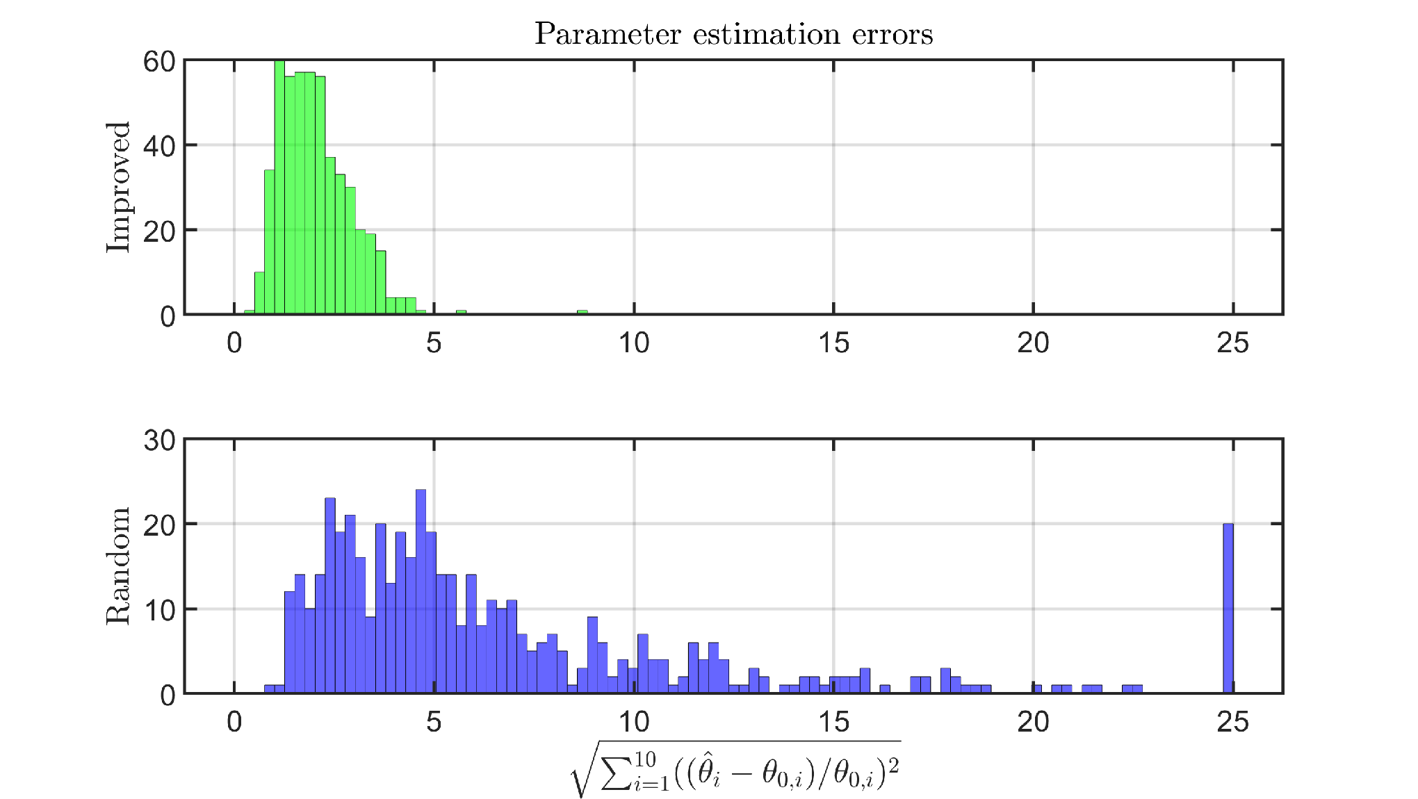
was used, which is able to describe the data-generating system in undisturbed conditions. As discussed earlier, the instruments were generated by simulating the output of this model with crude parameter values $\bm{\theta}^{\prime}$ ($\theta^{\prime}_{1}=\theta^{\prime}_{5}=-0.08$, $\theta^{\prime}_{4}=\theta_{7}=10^{-5}$, $\theta^{\prime}_{8}=-0.4$, $\theta^{\prime}_{10}=3.5\cdot 10^{-4}$ and $\theta^{\prime}_{2}=\theta^{\prime}_{3}=\theta^{\prime}_{6}=\theta^{\prime}_{9}=0$). As discussed before, the accuracy of an IV estimator is highly dependent on the instruments and a too imprecise nominal model can make the estimator diverge. Despite neglecting all nonlinear effects, the nominal model above was sufficiently accurate to yield a reliable estimator. Further, an optimized input sequence of 125 s (1000 samples) was formed, which respected the found ratios and new data was collected where $u_{c}(k)\sim\mathcal{N}(0,0.025)$, $v_{c}(k)\sim\mathcal{N}(0,0.025)$ and $e_{i}(k)\sim\mathcal{N}(0,0.025)$ for $i=1,2,3$. The models obtained from 500 Monte Carlo simulations using this optimized design were compared with models obtained using a random design. The random design was formed by arbitrarily choosing 1 out of the 11 input signals for each of 5 equally long segments (200 samples each). Which input signals that were used and in what order, was varied over the Monte Carlo simulations. For each Monte Carlo iteration, parameter estimation errors were computed and ideally, histograms showing these individually would be provided. Instead, due to limited space, a normalized root-mean-squared error (RMSE) for each estimated parameter was computed and the norm of all these is shown in Figure 1. By visual inspection it can be seen that the random design often gives higher estimation errors and that the improved design is a more robust choice in this regard. The improved design gives an error that is smaller than 5 in more than 99 % of the cases, whereas the random design only does so in 49 % of the cases.

The accuracies of the estimated models were also evaluated by cross-validation (CV) between simulated model output and the output of the true system. In the validation dataset, an input signal that was different from all the experiment primitives was used. The RMSE metric was used in this case as well and in Figure 2, the errors for each DOF is shown and in Figure 3, the norm of these is shown. It can be seen that the simulated model output is more often in agreement with the system output when the optimized experiment design is used. Similar to when parameter errors were considered, it can in Figure 3 be noted that the norm of the simulation errors is smaller than 0.15 in 99 % of the cases when the optimized design is used but only in 69 % of the cases when the random design is used. Similar observations can be made for each individual DOF in Figure 2.

Experimental data was also collected using a small-scale surface ship, which is about 1 meter long, 0.3 meter wide and weighs roughly 14 kg. This ship is actuated by two azimuth thrusters mounted in the aft and a tunnel thruster located in the bow. Further, the ship is equipped with an inertial measurement unit (IMU) for orientation, a GNSS receiver for positioning, as well as rotational-speed sensors for the thrusters. The surge and sway speeds were estimated using Euler’s explicit method with the position and orientation measurements. In order to make the analysis simple, the tunnel thruster was not used during the experiments and the input forces and moments, $\tau_{1}(k)$, $\tau_{2}(k)$ and $\tau_{3}(k)$, were generated solely based on the two azimuth thrusters. A simple static model for describing forces and moments obtained from azimuth thrusters is

where $l_{x,i}$ and $l_{y,i}$ define the (known) mounting position of azimuth thruster $i$ in $x$ and $y$-direction, respectively. The control signals, $n_{1}(k)$, $n_{2}(k)$, $\alpha_{1}(k)$ and $\alpha_{2}(k)$, were based on this model chosen to yield experiment primitives in agreement with the simulation experiments shown above. Moreover, the model structure was the same as in the simulation experiments and the instruments were again generated by use of a nominal model. This time, the crude parameter values used for the nominal model were obtained by the least-squares estimate, $i.e.$, by letting $\bm{Z}(k)=\bm{\Phi}(k)$.

The collected data was divided into 55 parts (75 samples each), 5 for each of the 11 experiment primitives. Using these shorter datasets for estimating (26)-(28) and solving (29), gave an optimized design where $\bm{\tau_{1}}(k)$ is used for $20~\%$ of the total experiment time, $\bm{\tau_{6}}(k)$ for $49~\%$, $\bm{\tau_{9}}(k)$ for $13~\%$ and $\bm{\tau_{11}}(k)$ for $18~\%$. This optimized design was then approximated with a design where $\bm{\tau_{6}}(k)$ is used for half of the total time and $\bm{\tau_{1}}(k)$, $\bm{\tau_{9}}(k)$ and $\bm{\tau_{11}}(k)$ are used for one sixth of the time each. In this way, multiple different datasets could be formed from the collected data where the optimized ratios were fulfilled. The fact that multiple different realizations of the optimal experiment could be formed made it easier to discuss the results and to make statistical conclusions, something that is otherwise only possible in simulation experiments where more data is available.

The optimized datasets were formed by picking 3 sub-experiments where $\bm{\tau_{6}}(k)$ is used and 1 sub-experiment where $\bm{\tau_{1}}(k)$, $\bm{\tau_{9}}(k)$ and $\bm{\tau_{11}}(k)$ are used each, $i.e.$, 6 shorter sub-experiments were used in total. This way of forming the experiment was compared to a random design, where 6 sub-experiments were selected randomly. Similarly to the simulation experiments, the accuracies of the estimated models were evaluated by CV between simulated model output and estimates obtained from the measured signals. For both the optimized design and the random design, the set of sub-experiments was varied 500 times and the results are given in Figures 4 and 5. It can be seen that the simulated model output is more often in agreement with the measured system output when the optimized experiment design is used. Here, it is most notable because the error following the random design takes on degenerate values in about 20 % of the cases.

The validation data was made up by all the 55 sub-experiments, which means that the validation data was not completely independent of the estimation data ($6/55\approx 11~\%$ overlap). This small overlap was deemed justifiable because the alternative would be a folded type of CV, where the sub-experiments currently used for estimation were kept out and not included in the validation set. Since there were only 5 sub-experiments of each type available, this would mean that some maneuvers occasionally were not present at all in the validation data and would therefore possibly result in a misleading evaluation.

There was also data available from a full-scale ship. This ship is roughly 30 meters long and has an actuator setup with two azimuth thrusters mounted along the centerline, one at the front and one in the rear. This configurations makes it possible to excite the ship in sway without having a forward speed. The full-scale ship is equipped with a GNSS receiver with two antennas, which provides estimates of both its position and yaw angle. Unlike the small model ship discussed before, all signals were sampled at the lower rate of $f_{s}=1$ Hz. Notably, the data from the full-scale ship was not collected for the sake of this work in particular and consequently the data does not include the previously discussed experiment primitives. Instead, the following motion types were identified.

1. ($\bm{\tau}_{12}$)

   Surge accelerations/decelerations:
   $u(k)\in[0,3.5]$, $v(k)=0$, $r(k)=0$.

2. ($\bm{\tau}_{13}$)

   Sway accelerations/decelerations:
   $u(k)=0$, $v(k)\in[-1,1]$, $r(k)=0$.

3. ($\bm{\tau}_{14}$)

   Slow sway motion:
   $u(k)=0$, $\mathinner{\!\left\lvert v(k)\right\rvert}\in[0.5,0.8]$, $r(k)=0$.

4. ($\bm{\tau}_{15}$)

   Moderate sway motion:
   $u(k)=0$, $\mathinner{\!\left\lvert v(k)\right\rvert}\approx 0.9$, $r(k)=0$.

5. ($\bm{\tau}_{16}$)

   Fast sway motion:
   $u(k)=0$, $\mathinner{\!\left\lvert v(k)\right\rvert}\in[1.1,1.2]$, $r(k)=0$.

6. ($\bm{\tau}_{17}$)

   Slow/high frequent ($T\approx 30$) zig-zag motion:
   $u(k)\approx 3$, $v(k)\in[-0.5,0.5]$, $r(k)=\in[-0.03,0.03]$.

7. ($\bm{\tau}_{18}$)

   Fast/high frequent ($T\approx 30$) zig-zag motion:
   $u(k)\approx 4$, $v(k)\in[-0.5,0.5]$, $r(k)=\in[-0.03,0.03]$.

8. ($\bm{\tau}_{19}$)

   Slow/low frequent ($T\approx 100$) zig-zag motion:
   $u(k)\approx 3$, $v(k)\in[-0.5,0.5]$, $r(k)=\in[-0.03,0.03]$.

9. ($\bm{\tau}_{20}$)

   Fast/low frequent ($T\approx 100$) zig-zag motion:
   $u(k)\approx 4$, $v(k)\in[-0.5,0.5]$, $r(k)=\in[-0.03,0.03]$.

As before, all values for $u(k)$ and $v(k)$ are given in m/s and the values for $r(k)$ in rad/s. Moreover, $T$ is the period time of the zig-zag motion in seconds. The simple model structure (30) turned out to be sufficient for describing the collected data and was therefore used here as well and the instrument matrix was generated in the same way as for the small-scale ship. Further, the data was divided into different parts for the different maneuvers. This time, 4 sub-experiments of each type were formed, each corresponding to 100 seconds of maneuvering ($i.e.$, 100 samples). Estimating (26)-(28) and solving (29) gave an optimized design where $\bm{\tau_{13}}(k)$ is used for $4~\%$ of the total experiment time, $\bm{\tau_{14}}(k)$ for $2~\%$, $\bm{\tau_{16}}(k)$ for $30~\%$, $\bm{\tau_{18}}(k)$ for $22~\%$, $\bm{\tau_{19}}(k)$ for $11~\%$ and $\bm{\tau_{20}}(k)$ for $31~\%$.

Analogously to before, the optimal design was approximated with a design where $\bm{\tau_{16}}(k)$ and $\bm{\tau_{20}}(k)$ are used for one third each while $\bm{\tau_{18}}(k)$ and $\bm{\tau_{19}}(k)$ are used for one sixth each. In this case, realizations of an optimal experiment can be formed by picking 2 of the sub-experiments where $\bm{\tau_{16}}(k)$ is used, 1 where $\bm{\tau_{18}}(k)$ is used, 1 where $\bm{\tau_{19}}(k)$ is used and 2 where $\bm{\tau_{20}}(k)$ is used. Furthermore, the optimized experiment design was compared with a random design, where 6 sub-experiments were selected randomly and the accuracies of the estimated models were evaluated by CV between simulated model output and estimates obtained from the measured signals. For both the optimized design and the random design, the set of sub-experiments was varied 500 times and the results are given in Figures 6 and 7. Here it is actually the case that the most accurate models are obtained with the random design. The worst-case errors following the random design are, however, also higher and sometimes take on degenerate values. In this sense, the optimized design is a more solid choice.

It can be remarked that the data from the full-scale ship was collected on two separate occasions with quite different weather conditions. Parts of the data was collected during a day with wind speeds of less than 3 m/s, $i.e.$ light breeze by the definition in [8], whereas the other parts were collected during a day where the wind speed was about 10 m/s, which corresponds to fresh breeze by the same set of definitions. Further, $\bm{\tau_{16}}(k)$-$\bm{\tau_{18}}(k)$ were only applied during the windy day and consequently, the data associated with those experiment primitives is more noisy in comparison to the other data. Due to the way that the realizations of the optimal design are formed, by concatenation of sub-experiments where both $\bm{\tau_{16}}(k)$ and $\bm{\tau_{18}}(k)$ are used, they are bound to always include at least $50~\%$ of data from the windy day. The realizations of the random design are, however, occasionally made up exclusively of data from the calmer day, which partly explains why the most accurate models are obtained with the random design.

References

- [1] Martin A. Abkowitz. Lectures on ship hydrodynamics – steering and manoeuvrability. Technical Report HY-5, Hydro- and Aerodynamics Laboratory, Lyngby, Denmark, 1964.
- [2] Kristoffer Bergman. Exploiting Direct Optimal Control for Motion Planning in Unstructured Environments. PhD thesis, Linköpings universitet, Linköping, Sweden, 2021.
- [3] Mogens Blanke and Morten Knudsen. Optimized experiment design for marine systems identification. In Proceedings of the 14th IFAC World Congress, pages 8249–8254, Beijing, China, 1999.
- [4] Mogens Blanke and Morten Knudsen. Efficient parameterization for grey-box model identification of complex physical systems. In 14th IFAC Symposium on System Identification (SYSID), pages 338–343, Newcastle, Australia, 2006.
- [5] Alexander De Cock, Michel Gevers, and Johan Schoukens. D-optimal input design for nonlinear FIR-type systems: A dispersion-based approach. Automatica, 73:88–100, 2016.
- [6] K. K. Fedyaevsky and G. V. Sobolev. Control and stability in ship design. State Union Ship-building House, St. Petersburg, Russia, 1964.
- [7] Marco Forgione, Xavier Bombois, Paul M. J. Van den Hof, and Håkan Hjalmarsson. Experiment design for parameter estimation in nonlinear systems based on multilevel excitation. In European Control Conference (ECC), pages 25–30, 2014.
- [8] Thor I. Fossen. Handbook of marine craft hydrodynamics and motion control. John Wiley & Sons, Chichester, U.K., 2011.
- [9] László Gerencsér, Håkan Hjalmarsson, and Jonas Mårtensson. Identification of arx systems with non-stationary inputs—asymptotic analysis with application to adaptive input design. Automatica, 45(3):623–633, 2009.
- [10] Michel Gevers, Xavier Bombois, Roland Hildebrand, and Gabriel Solari. Optimal experiment design for open and closed-loop system identification. Communications in Information and Systems, 11(3):197–224, 2011.
- [11] Graham C. Goodwin and Robert L. Payne. Dynamic system identification: experiment design and data analysis. Mathematics in science and engineering, 136, 1977.
- [12] R. Bhushan Gopaluni, Thomas B. Schön, and Adrian G. Wills. Input design for nonlinear stochastic dynamic systems–a particle filter approach. In Proceedings of the 18th IFAC World Congress, pages 13191–13196, Milano, Italy, 2011.
- [13] Håkan Hjalmarsson and Jonas Mårtensson. Optimal input design for identification of non-linear systems: Learning from the linear case. In American Control Conference (ACC), pages 1572–1576, 2007.
- [14] Sven Lack, Erik Rentzow, and Torsten Jeinsch. Experimental parameter identification for an open-frame ROV: Comparison of towing tank tests and open water self-propelled tests. IFAC-PapersOnLine, 52(21):271–276, 2019.
- [15] Christian A. Larsson, Håkan Hjalmarsson, and Cristian R. Rojas. On optimal input design for nonlinear FIR-type systems. In 9th IEEE Conference on Decision and Control (CDC), pages 7220–7225, Atlanta, GA, USA, 2010.
- [16] Lennart Ljung. System identification: theory for the user (2nd edition). Prentice Hall, Upper Saddle River, N. J., 1999.
- [17] Fredrik Ljungberg and Martin Enqvist. Consistent estimators for nonlinear vessel models. arXiv:2204.04973, 2022.
- [18] Kaushik Mahata, Johan Schoukens, and Alexander De Cock. Information matrix and D-optimal design with Gaussian inputs for Wiener model identification. Automatica, 69:65–77, 2016.
- [19] Raman Mehra. Optimal input signals for parameter estimation in dynamic systems–survey and new results. IEEE Transactions on Automatic Control, 19(6):753–768, 1974.
- [20] Nicolas Minorsky. Directional stability of automatically steered bodies. Journal of the American Society for Naval Engineers, 34(2):280–309, 1922.
- [21] Nowrouz Mohammad Nouri, Mehrdad Valadi, and Jafar Asgharian. Optimal input design for hydrodynamic derivatives estimation of nonlinear dynamic model of AUV. Nonlinear Dynamics, 92(2):139–151, 2018.
- [22] Mihail Pivtoraiko, Ross A. Knepper, and Alonzo Kelly. Differentially constrained mobile robot motion planning in state lattices. Journal of Field Robotics, 26(3):308–333, mar 2009.
- [23] Stéphane Thil, Marion Gilson, and Hugues Garnier. On instrumental variable-based methods for errors-in-variables model identification. In Proceedings of the 17th IFAC World Congress, pages 426–431, Seoul, Korea, 2008.
- [24] Jack Umenberger and Thomas B. Schön. Nonlinear input design as optimal control of a Hamiltonian system. IEEE Control Systems Letters, 4(1):85–90, 2019.
- [25] Patricio E. Valenzuela, Johan Dahlin, Cristian R. Rojas, and Thomas B. Schön. On robust input design for nonlinear dynamical models. Automatica, 77:268–278, 2017.
- [26] Patricio E. Valenzuela, Cristian R. Rojas, and Håkan Hjalmarsson. A graph theoretical approach to input design for identification of nonlinear dynamical models. Automatica, 51:233–242, 2015.
- [27] Tyrone L. Vincent, Carlo Novara, Kenneth Hsu, and Kameshwar Poolla. Input design for structured nonlinear system identification. Automatica, 46(6):990–998, 2010.
- [28] Zihao Wang, C. Guedes Soares, and Zaojian Zou. Optimal design of excitation signal for identification of nonlinear ship manoeuvring model. Ocean Engineering, 196:106778, 2020.
- [29] Erik Wernholt and Johan Löfberg. Experiment design for identification of nonlinear gray-box models with application to industrial robots. In 46th IEEE Conference on Decision and Control (CDC), pages 5110–5116, New Orleans, LA, USA, 2007.
- [30] Erik Wernholt and Stig Moberg. Nonlinear gray-box identification using local models applied to industrial robots. Automatica, 47(4):650–660, 2011.
- [31] Hyeon Kyu Yoon and Key Pyo Rhee. Identification of hydrodynamic coefficients in ship maneuvering equations of motion by estimation-before-modeling technique. Ocean Engineering, 30(18):2379–2404, 2003.