Arrasy Rahman, Ignacio Carlucho, Niklas Höpner and Stefano V. Albrecht
A General Learning Framework for Open Ad Hoc Teamwork Using Graph-based Policy Learning
Abstract
Open ad hoc teamwork is the problem of training a single agent to efficiently collaborate with an unknown group of teammates whose composition may change over time. A variable team composition creates challenges for the agent, such as the requirement to adapt to new team dynamics and dealing with changing state vector sizes. These challenges are aggravated in real-world applications in which the controlled agent only has a partial view of the environment. In this work, we develop a class of solutions for open ad hoc teamwork under full and partial observability. We start by developing a solution for the fully observable case that leverages graph neural network architectures to obtain an optimal policy based on reinforcement learning. We then extend this solution to partially observable scenarios by proposing different methodologies that maintain belief estimates over the latent environment states and team composition. These belief estimates are combined with our solution for the fully observable case to compute an agent’s optimal policy under partial observability in open ad hoc teamwork. Empirical results demonstrate that our solution can learn efficient policies in open ad hoc teamwork in fully and partially observable cases. Further analysis demonstrates that our methods’ success is a result of effectively learning the effects of teammates’ actions while also inferring the inherent state of the environment under partial observability.11 1 We provide an implementation of the algorithms and the environments in https://github.com/uoe-agents/PO-GPL
keywords
ad hoc teamwork, reinforcement learning, partial observability, graph neural networks, particle filter1 Introduction
Current research in multi-agent systems has demonstrated how teams of agents can be co-trained to learn policies to solve a number of problems, such as smart grid management (Roesch et al. 2020), navigating human-shared environments (Boldrer et al. 2022), multi-robot warehouse management (Krnjaic et al. 2023), and real-time strategy games (Zhou et al. 2021). In many real-world applications, a controlled agent may be required to collaborate in diverse teams without the possibility of previous joint training. This problem is commonly referred to as ad hoc teamwork (Stone et al. 2010). The objective of ad hoc teamwork is to train a single agent, which we refer to as the learner, that can successfully collaborate “on the fly” with a group of teammates with unknown policies. Previous research on ad hoc teamwork has focused on the application of agent modelling (Barrett et al. 2012; Albrecht and Stone 2018) or communication techniques (Mirsky et al. 2020; Mirsky et al. 2022). However, most prior ad hoc teamwork approaches are based on assumptions which may not hold in real-world applications.
One of these assumptions is that the number of other agents in the team is fixed. Real-world scenarios, such as autonomous driving and robotics rescue tasks, may require the learner to interact with a changing number of agents between timesteps. In open ad hoc teamwork, teammates may enter or leave the environment without prior notification. We refer to the variable team size nature as open teams or environmental openness (Eck et al. 2020). The open nature of the team presents a set of additional challenges to the learner, which increases the difficulty of the ad hoc teamwork task. We call the problem of designing an ad hoc teamwork learner in open teams the open ad hoc teamwork problem.
There are two main challenges in solving open ad hoc teamwork. The first challenge that needs to be addressed is the change in the size of the observation vector resulting from teammates entering or leaving the environment, which prevents many function approximation models that assume fixed input sizes from being directly applicable to estimating the learner’s optimal policy. Second, the unknown team composition resulting from teammates joining or leaving the environment requires the learner to rapidly adapt its policy to effectively collaborate with its teammates. For instance, the learner may need to adopt different roles when dealing with teams that consist of distinct collections of teammate behavioural policies (Mirsky et al. 2022).
Another commonly violated assumption in real-world ad hoc teamwork problems is related to state information availability. In many problems, agents only have access to observations containing partial information of the state. The learner then has to infer the latent environment state based only on a sequence of partial observations. The combination of partial observability and open ad hoc teamwork provides new challenges to the learner, which now has to model the effects of environment openness while also inferring the latent state of the environment. Since the actions taken by other agents can affect the learner’s returns, the learner also needs to maintain a model of all existing teammates’ actions, even for unobserved teammates. Previous works have addressed the ad hoc teamwork problem under partial observability (Gu et al. 2021; Ribeiro et al. 2022), but have not considered team openness.
In this work, we investigate approaches for solving the challenges introduced by open ad hoc teamwork under full and partial observability. First, we present different algorithms that solve the fully observable open ad hoc teamwork problem. Our algorithms are based on three main components that a learner requires for effective ad hoc collaboration with teams of variable sizes. These three components are respectively used for teammate type inference, action prediction, and joint action value modelling. The output of these three components can be combined together to estimate a learner’s optimal policy for open ad hoc teamwork. To deal with environment openness, we implement these components as GNN (GNN) architectures, which have been demonstrated as effective function approximation models for input data with variable sizes (Jiang et al. 2019; Huang et al. 2020). We call our proposed learning framework GPL (GPL) and we demonstrate GPL’s ability to train a learner’s optimal policy in fully observable open ad hoc teamwork problems.
Our results show that a GPL-based learner achieves significantly higher returns in open ad hoc teamwork than learners that use value-based reinforcement learning and multi-agent reinforcement learning algorithms for training. Furthermore, a GPL-based learner also achieves significantly higher performance compared to baseline methods when evaluated under an open process it has not experienced during training. Our experiments demonstrate that GPL’s significantly higher performance results from its usage of GNNs and joint action value modelling, which enables GPL to learn the effects of other teammates’ actions towards the learner. Through additional experiments we empirically demonstrate that learning the effects of teammates’ actions via the joint action value model enables a learner to acquire useful behaviour from teammates.
We then address the open ad hoc teamwork problem under partial observability by extending GPL with belief inference methods that estimate the latent environment state. We evaluate different belief inference methods which allow the learner to maintain representations of important latent variables for decision making, such as the environment state, teammates’ existence, as well as teammates’ joint actions. The belief inference methods proposed in this work are inspired by latent variable inference methods such as SMC (SMC) methods (Doucet et al. 2001), autoencoders (Rumelhart et al. 1985), and variational autoencoders (Kingma and Welling 2013). We enable the proposed belief inference methods to handle data resulting from variable team sizes by using GNN-based models and graph generation techniques. Additionally, our extension to partial observability utilises the representations from the belief inference model as inputs to the different modules in GPL to estimate the learner’s optimal policy.
We evaluate the performance of the different proposed belief inference models when combined with GPL to solve partially observable open ad hoc teamwork problems. Additionally, we compare the combination of GPL with the proposed belief inference models against different single-agent RL baselines Schulman et al. 2017; Igl et al. 2018. Our results show that autoencoder-based belief inference models achieve significantly higher returns than the other proposed methods and baselines in the different evaluated environments. Further investigation into the information encoded by the belief inference models demonstrates that using autoencoder-based architectures yields representations that more accurately encode the latent environment state and teammates’ joint actions. This improved representational quality enables the learner to achieve higher returns when using the resulting representations for decision-making under partial observability. We also investigate the proposed belief inference models’ ability to encode the existence of teammates not perceived in the partial observation. Our results demonstrate that SMC-based methods are significantly more effective at encoding unobserved teammates’ existence. However, these methods do not translate to higher returns during decision-making, since SMC-based representations are unable to accurately represent the latent environment state and teammates’ joint actions. On the other hand, our generalisation results show that autoencoder-based architectures are able to generalise better to different numbers of teammates, as well as to previously unseen teammates during training.
The remainder of this paper introduces our proposed methods and details our experiments in open ad hoc teamwork. In Section 2 we discuss related works, followed by Section 3 which formalises the learning problem in open ad hoc teamwork. Section 4 introduces GPL as a method for solving the open ad hoc teamwork problem under full observability. We then describe our fully observable open ad hoc teamwork experiments and analyse the results from GPL in Section 5. Section 6 then presents different methodologies to solve the open ad hoc teamwork problem under partial observability, which is followed by the description of our experiments under this setting alongside the analysis of its associated results in Section 7. Finally, we summarise our findings in this work and provide pointers to potential future work in Section 8.22 2 Parts of this work have previously been published by Rahman et al. 2021. This new version includes a new formal model for open ad hoc teamwork under partial observability alongside new algorithms and experimental results that are specifically designed to deal with partial observability.
2 Related Work
Ad Hoc Teamwork. Ad hoc teamwork is the problem of training a single agent to perform optimally in a team of unknown teammates (Stone et al. 2010). Three main assumptions characterise ad hoc teamwork (Mirsky et al. 2022). First is the lack of prior coordination between agents. This means that the learner should be able to cooperate with the team on-the-fly, without the opportunity to rely on previously agreed collaboration strategies. The second assumption is the fact that the learner has no control over its teammates. Lastly, teammates are assumed to be collaborative. That is, all agents in the team have a common goal and are able to take actions that will benefit the team. However, teammates might have additional objectives, that may vary per teammate, and even have different rewards. Early works in ad hoc teamwork operated under the assumption that the teammate’s behaviour was known to the learner (Stone and Kraus 2010; Agmon and Stone 2012). Other approaches have relaxed this restrictive assumption from these early works and assumed teammate behaviour to be unknown during the interaction. These approaches (Albrecht and Stone 2017; Barrett et al. 2017) proposed methods that infer teammates’ policy based on their displayed behaviour and utilise it for decision making. Such methods typically utilise the concept of types, which encapsulates the important information determining an agent’s behaviour. In type-based methods, each teammate’s behaviour is assigned a particular hypothesised type (Albrecht et al. 2016). Then during the interaction, new unseen teammates are assigned one of the previously hypothesised types (Ravula et al. 2019; Mirsky et al. 2020). One issue with these methods is that during training they require diverse teammates, to allow the ad hoc agent to learn policies that are useful for collaborating with novel partners. Current research has thus focused on how to generate diverse teammates for ad hoc teamwork training (Rahman et al. 2023b; Rahman et al. 2023a). Another avenue of research within ad hoc teamwork focuses on how communication can be leveraged inside the team to improve the overall performance (Barrett et al. 2014; Macke et al. 2021). However, all these prior works assume that the teams are closed, meaning that the number of teammates and their types are fixed during episodes. A very limited number of works consider the case of open ad hoc teamwork, which poses an even more difficult problem (Chandrasekaran et al. 2016).
Recent works have addressed the ad hoc teamwork problem under partial observability. Gu et al. 2021 presented ODITS, a reinforcement learning-based approach, which utilises an information-based regulariser to estimate proxy representations based solely on the learner’s observations. Recently, Ribeiro et al. 2022 presented a Bayesian prediction algorithm for addressing partial observability in ad hoc teamwork. However, these works only considered closed teams. Unlike previous works, our proposal is the first to address the open ad hoc teamwork problem under partial observability.
Zero-Shot Coordination. A related problem to ad hoc teamwork is that of zero-shot coordination (ZSC) (Hu et al. 2020). In ZSC agents are paired together and need to coordinate on-the-fly. However, in ZSC reward functions are assumed to be the same across the different agents, while our definition of ad hoc teamwork assumes that the learner has no specific knowledge about the rewards of other agents (Mirsky et al. 2022). Initial works in ZSC proposed an updated version of self-play, called other-play, that aims to break symmetries in MDPs to improve coordination. Other works have focused on how to generate teammates that have diverse policies (Lupu et al. 2021; Rahman et al. 2023b).
Belief States. Many approaches to find optimal policies for a POMDP are based on computing a probability distribution, or a belief state, regarding the actual state of the learner (Izadi and Precup 2005; Albrecht and Ramamoorthy 2016; Albrecht and Ramamoorthy 2017). Other works have also suggested the use of RNN to deal with the uncertainty in the observations (Wierstra et al. 2007; Hausknecht and Stone 2015). However, these models are incapable of modelling the learner’s uncertainty of the latent state due to only modelling the latent state as a single representation. A different approach was taken by Coquelin et al. 2009, which proposed the use of a particle filter (or sequential Monte-Carlo) (Arulampalam et al. 2002) for estimating the belief state in POMDP. More recently, Le et al. 2018 solved issues of belief update using variational autoencoders trained by optimising ELBO (ELBO). These improvements were later leveraged for estimating belief states in single agent POMDP (Igl et al. 2018; Singh et al. 2021).
Interactive POMDPs (I-POMDPs). Interactive POMDPs are an extension of POMDPs to the multi-agent domain (Doshi and Gmytrasiewicz 2011). It achieves this by including agent models in the state space. As such, I-POMDPs are related to SBG (Albrecht et al. 2016), however, I-POMDPs have mostly focused on the nested belief which makes their solutions complex. Chandrasekaran et al. 2016 leveraged instead I-POMPD-Lite (Hoang and Low 2013), a simplified version of I-POMDPs that assumes the behaviour of other agents follows a nested MDP, for solving the planning problem in open multi-agent systems. Our problem formulation is instead based on SBG, which utilises the joint action to model the effects of teammates in the observations of the agent (Albrecht et al. 2016).
Graph Neural Networks (GNNs). GNNs are a newly proposed type of neural network that can work with graph-structured data (Wu et al. 2019). GNN have been used for solving a diverse domain of problems, such as chemical reaction prediction (Do et al. 2019), generative models (Grover et al. 2019) or traffic prediction (Zheng et al. 2020). In multi-agent settings, GNN have been used for modelling other agents’ behaviour (Tacchetti et al. 2018), although only in closed environments. In MARL (MARL), GNN (Boehmer et al. 2020; Naderializadeh et al. 2020) have been used to factorise value functions (Guestrin et al. 2002a) as CG. Deep CG have also been used in ad hoc teamwork (Rahman et al. 2021), although under full observability.
Multi-agent Reinforcement Learning (MARL). MARL explores the application of reinforcement learning to jointly train a collection of agents, whose goal is to maximise their individual returns in each other’s presence (Albrecht et al. 2023). Previous MARL approaches have focused on ideas such as counterfactual credit assignment (Foerster et al. 2018), joint action value factorisation (Sunehag et al. 2017; Rashid et al. 2018; Boehmer et al. 2020), and learning communication protocols between agents (Foerster et al. 2016; Jiang et al. 2019). MARL differs from ad hoc teamwork in two aspects. First, MARL approaches assume control over a set of agents during training and execution, whereas ad hoc teamwork only assumes control over the learner. Second, MARL assumes that an agent will only interact with other agents encountered during joint training, while ad hoc teamwork methods neither assumes knowledge nor control over the teammates that are encountered during evaluation. As a result of these differences, MARL has previously been demonstrated to yield poor performances when dealing with teammate policies not encountered during training (Vezhnevets et al. 2020; Hu et al. 2020), which we also show in our experiments.
3 Problem Formulation
A formal model for ad hoc teamwork must achieve two requirements. First, the model must formalise the interaction between agents and the effects these interactions have towards the information perceived by the learner. Second, these models must represent the absence of knowledge regarding teammates’ decision-making process.
The SBG (SBG) model (Albrecht et al. 2016) fulfils the aforementioned requirements by combining the Stochastic Game (Shapley 1953) and Bayesian Game model (Harsanyi 1967). Using the formalism defined in Stochastic Games, SBG formally models the effects of the agents’ joint actions on the learner’s observed states and rewards. At the same time, SBG adopts the concept of types from Bayesian Games to encapsulate the set of unknown information regarding teammates’ decision making process.
While SBG adequately formalise ad hoc teamwork where team sizes are fixed, they are insufficient for open ad hoc teamwork due to their inability to formalise the changing number of teammates. To address the limitations of the SBG model as a formal definition of open ad hoc teamwork, we introduce the OSBG (OSBG) model. OSBG extends the SBG model to open environments by adding components that formalise the changing number of teammates. Additionally, we present an extension of OSBG, that formalises the ad hoc teamwork problem under partial observability, the PO-OSBG (PO-OSBG) model. We introduce the OSBG model in Section 3.1, and in Section 3.2 we specify the learner’s learning objective when solving an open ad hoc teamwork problem under the proposed OSBG. We then introduce the PO-OSBG extension in Section 3.3, and present the learning objectives when solving open ad hoc teamwork problems under partial observability in Section 3.4.
3.1 Open Stochastic Bayesian Games (OSBG)
In this section, we define the OSBG (OSBG) model, which is an extension of SBG that formalises the open ad hoc teamwork problem.33 3 This model definition appeared originally in Rahman et al. 2021. We define OSBG as follows:
Definition 1.
An OSBG, is a 7-tuple containing the following components:
- •
The finite state space.
- •
The finite set of possible actions for each agent44 4 is assumed to be shared between agents for simplicity. This can be extended to cases where agents’ action spaces are different by assuming that is the union of all agents’ individual action spaces..
- •
The finite set of types that can be assumed by teammates.
- •
The finite set of possible agents, .
- •
The discount rate.
Before defining the remaining components of an OSBG, we first introduce notations regarding the agent type assignment and action selection under a variable number of agents. Note that a valid action selection and type assignment only allows an agent to be associated with a single type and action. Assuming , , and denote the power set of set , action selected by agent , and type assigned to agent , respectively, we define notations for valid agent type and action assignments as follows:
- •
denotes the joint agent-action space, which is the set of all possible joint action selections under a variable number of agents. The predicates that define the membership of to ensure that each agent can only select a single action in a valid joint action selection. Its elements, , are referred as joint agent-actions.
- •
is the joint agent-type space, which denotes the set of all possible assignments of types under a variable number of agents. Similar to , the predicates in the membership conditions of ensures that each agent can only be assigned a single type. Its elements, , are then referred to as the joint agent-type. Each type in the joint agent-type represents a set of information or action selection mechanisms underlying a different existing agent’s behaviour. Note that during action selection, teammates’ types are unknown to the learner, since we do not assume knowledge over teammates’ types in ad hoc teamwork.
With the defined notation of and and with denoting the set of all probability distributions over a random variable , the remaining components of an OSBG are defined as follows:
- •
, which is the reward function that determines the rewards received by the learner, given the actions of all agents in the environment.
- •
, which is the transition function which determines the next state and joint agent-types encountered by the learner, given the current state, joint agent-types and joint agent-actions.
The interaction between a learner and its teammates in an OSBG starts from an initial state, . To model changing numbers of agents in the open environment, different subsets of agents are sampled from to model the set of existing agents in the environment at each timestep. At the beginning of the episode, the initial set of teammates, is sampled and assigned the joint agent-type . The initial state (), set of teammates (), and joint agent-type (), are sampled from the initial distribution . As an example, if the task would be to play a game of football then each type will correspond to a different policy that controls a teammate to play a specific position (e.g winger, defender, or striker) with different skill levels.
At each timestep, the interaction between the learner and its teammates undergoes two distinct processes. First, teammates select their respective actions according to the observed state of the environment at time . Each teammate selects its action based on its current policy, , conditioned on the state, the existing set of agents, and its assigned type. In the football example, each teammate will select their action based on their own sequence of observations. Meanwhile, the learner chooses its actions based on its sequence of previously observed states and executed actions, , without knowing teammates’ types or actions, which formalises the lack of knowledge regarding teammates’ decision-making process assumed by ad hoc teamwork problems. Unlike its teammates, the learner chooses its actions based on because it has no knowledge of its teammates’ types and must infer it through their observed behaviour throughout the interaction.
The second step occurs as a result of the execution of joint actions chosen by agents at the first step. Following the execution of the agents’ joint action, the learner receives a scalar reward, , which is determined by the reward function . The environment state, the set of existing teammates, and the joint agent-type all change following the transition function defined by . Aside from determining the next state observed by the learner, the transition function also models the way teammates may enter or leave the environment. This is done by determining the set of teammates encountered by the learner at the next timestep and alongside their respective types.
3.2 Learning Objective Under Full Observability
Solving an OSBG requires the learner, denoted by , to find an optimal policy, , which selects the optimal action based on the learner’s previously experienced environment states, observed teammates, and executed actions, . We define the optimal policy as follows:
Definition 2.
Let the joint actions and the joint policy of teammates at time be denoted by and , respectively. Given , and the learner’s previous experience, , we define the action-value of a policy , as:
| (1) |
A learner’s policy, , is then optimal if:
| (2) |
for all possible , , and . Given , a learner’s optimal policy is to greedily choose actions with the highest state-action value. Note that to remove any ambiguity in the text we use the bar notation to denote the action-value of the learner.
3.3 Partially Observable Open Stochastic Bayesian Games (PO-OSBG)
In this section, we define the PO-OSBG model, which is an extension of OSBG to problems with partial observability. PO-OSBG extends OSBG by introducing components which model the observations received by the learner during interaction with its teammates. We define the PO-OSBG model as follows:
Definition 3.
A PO-OSBG is an 9-tuple, consisting of the following components . In a PO-OSBG, , , and are defined exactly as their respective counterparts in an OSBG. The remaining components of a PO-OSBG which model the information received by the learner under partial observability are defined as follows:
- •
: The learner’s set of possible finite observations.
- •
), which is the observation function that determines the distribution of observations received by the learner given the current state of the environment and the learner’s set of teammates.
In a PO-OSBG, the interaction between a learner and its teammates is similar to their interactions in OSBGs. The main difference is that the learner will not perceive the subsequent state information after all agents execute their respective actions. Instead, at each timestep the learner receives an observation sampled from the distribution outputted by the observation function , which is determined by the state and set of teammates that exist in the environment at . This absence of state information forces the learner to choose actions based only on the sequence of observations and its actions until the present time, . On the other hand, teammates receive their own observations of the environment according to their own observation function. We assume that teammates’ observation functions are part of their type, and as a consequence unknown to the learner. This means that the PO-OSBG formulation defines the observation function only for the learner. The main reason behind this design is because many scenarios have learners that have different perception capabilities than its teammates. For instance, robots created from different factories may be equipped with different sets of sensors. Since teammates’ observation functions are unknown and important for their decision making process, the unknown observation function of teammates are instead encapsulated as part of their types under the PO-OSBG model.
3.4 Learning Objective Under Partial Observability
Solving a PO-OSBG amounts to finding an optimal policy for action selection based on the sequence of the learner’s previous observations and executed actions, . We define the optimal policy as follows:
Definition 4.
Let the unknown joint actions and the joint policy of teammates at time be denoted by and , respectively. Given , and , the action-value of a policy , is defined as:
| (3) |
A learner’s policy, , is then optimal if:
| (4) |
for all possible , , and . The learner’s optimal policy is to then greedily choose actions with the highest state-action value for any given experienced by the learner.
4 Open Ad Hoc Teamwork in Fully Observable Environments
We present here a general learning framework designed to achieve optimal decision-making in open ad hoc teamwork. We first provide a general overview regarding the role of the three main components that constitute our proposed method GPL (GPL). We then describe details of the models designed for each component, starting with the type inference component in Section 4.2, the joint action value modelling component in Section 4.3, and the agent modelling component in Section 4.4. Finally, Section 4.5 details the learner’s action selection process. and Section 4.6 outlines the learning objective for training GPL’s neural network-based components.
4.1 Overview
Our GPL (GPL) framework is based around three main components: a type inference model, a joint action value model, and an agent model, whose role in decision making is explained in the following sections. These components are trained to estimate the learner’s optimal policy using the experience collected by the learner while interacting with its teammates. The main components and interactions between them are illustrated in Figure 1.
The type inference model is needed to infer teammates’ unknown types in open ad hoc teamwork. Knowing teammates’ types is crucial for decision-making since it gives information regarding teammates’ selected actions, which can have a strong impact on the returns achieved by the learner. In the absence of knowledge regarding teammates’ inherent types, the type inference model infers each teammate’s type based solely on the sequence of past state features observed by the learner.
A joint action value model predicts the learner’s returns following existing agents’ joint actions. Modelling the joint action value is crucial to solving open ad hoc teamwork for two reasons. First, the agents’ joint actions influence the learner’s current and future rewards, following the reward and transition function definition in OSBGs. Second, the joint action value estimation provides better credit assignment than value-based RL methods that directly model the learner’s action-value function, such as Q-Learning (Watkins and Dayan 1992). Joint action value estimation prevents the agent from assigning too much credit to its action when it has minimal impact on the observed rewards, which has been demonstrated to be crucial for credit assignment in previous works related to MARL (Lowe et al. 2017; Foerster et al. 2018). In this work, we extend its applicability to ad hoc teamwork by incorporating a joint action value model as part of GPL. Section 5.3 shows that the joint action model contributes towards improved credit assignment, which enables the learner to identify and learn useful behaviour from well-performing teammates.
Given the joint agent-action , the joint-action value of a learner’s policy, , is defined as follows:
| (5) |
In contrast to Equation (1), this joint-action value denotes the learner’s expected returns after joint agent-action is executed after a history of previously observed states and actions , assuming other agents follow , while the learner follows . This value is directly influenced by the set of existing teammates and their respective types, which determines the joint action selected by the joint teammate policy . GPL accounts for the influence of existing teammate types to by incorporating the inferred teammate types when estimating this value.
It is not possible to use Equation (5) directly to decide the learner’s optimal action. Using the joint action value model to decide the learner’s optimal action requires knowledge about actions that will be selected by teammates, a fact that is unknown to the learner when deciding its own actions. Nonetheless, we can still use the joint action value estimate for decision-making by exploiting the following equation:
| (6) |
which expresses the learner’s action value function in terms of . Equation (6) dictates that the learner’s action value is the expected value of under the distribution of teammates’ actions. In problems with discrete possible actions, may therefore be computed by evaluating for all possible joint actions and computing their weighted average according to teammates’ joint action probability.
Equation (6), highlights the importance of the agent model, which is the third component of GPL. The agent model’s role is to estimate teammates’ joint action likelihood . Estimating the likelihood gives the learner predictions regarding which actions will be selected by the teammates, which enables the learner to use its joint action value model to compute . Note that the learner’s prediction regarding teammates’ actions is based on the environment state and the teammates’ inferred types. The use of state and inferred teammate types for action prediction follows from OSBG’s formulation of teammate’s decision-making process as outlined in Section 1. Definition 4.4 further details a model which predicts teammates’ actions based on the state and inferred teammates’ types.
In the following subsections, we will describe the models implemented for each of the aforementioned components. We start by describing the type inference model in Section 4.2, followed by a description of the joint action value model in Section 4.3, and of the agent model in Section 4.4. We then explain how the output of these models are combined for action selection in Section 4.5. Section 4.6 concludes our method description by outlining the learning objective for training the defined models based on the learner’s experience interacting with teammates. Additionally, we present in Algorithm 1 a simplified pseudocode of GPL. A more detailed pseudocode can be found in Appendix A.
4.2 Type Inference
There are three challenges in designing type inference models for open ad hoc teamwork. First, the model must accurately predict the teammates’ types, even when interacting with previously unseen teammates. Second, the model must learn without ground truth knowledge regarding the current types of other members of the team. Third, the model should be able to handle inputs of different sizes, since the number of agents can vary between timesteps. In many real-world applications of ad hoc teamwork, the first two challenges result from the absence of any type-related information pertaining to teammates. For instance, obtaining ground truth types and knowledge of the wide-ranging type space of human agents can be difficult in applications of ad hoc teamwork to human-robot interaction. The third challenge is directly related to the problem of openness in ad hoc teamwork.
We address the aforementioned challenges by representing teammate types as continuous vectors. To compute such vectors we utilise RNN, which are trained to produce similar type vectors for teammates that have similar behaviour to each other. The RNN infers the current teammates’ type based on the input vector and the RNN hidden states. In this way, the current inferred type not only depends on the current observed state but on the sequence of observed behaviour for each teammate. As a result, the type inference model can be trained without ground truth teammate types while also generalising well against unseen teammates if the learner has previously interacted with teammates displaying similar behaviour.
The type inference model is implemented as a LSTM (LSTM) network (Hochreiter and Schmidhuber 1997) with parameters are denoted by . Assuming that and are the hidden and cell states of the LSTM at timestep , the LSTM updates the type vectors following this expression:
| (7) |
where is an input batch that contains information about the current state of the system. This LSTM-based type update is illustrated on the left side of Figure 1.
After the update process, additional steps are required to ensure only type vectors of existing agents are used in GPL’s optimal action value estimation. Between subsequent timesteps, the type inference model removes the type vectors of teammates that are no longer in the environment due to environment openness. At the same time, type vectors of newly-arrived teammates are added. More details on how state information is preprocessed and post-processed are given in Appendix C.1.
The parameters of the type inference network are optimised by back-propagating the losses from the agent model and the joint action value network. In practice, we utilise two separate networks, one that feeds the Joint Action Value model and one that feeds the Agent Model. This is done to avoid the losses from each model interfering during training. More details on how these losses are computed are given in Section 4.6 and in Appendix C.1.
4.3 Joint Action Value Model
A joint action value model for open ad hoc teamwork must address three challenges. First, the model must be capable of handling inputs of variable sizes resulting from environment openness. Second, it must facilitate efficient computation of the learner’s action value function based on Equation (6). Third, the model must also estimate the effects of teammates’ actions towards the learner’s returns.
One way to fulfil the aforementioned requirements is to represent the joint action value model as a fully connected CG (CG) (Guestrin et al. 2002b). CGs facilitate the factorisation of joint action value functions into singular and pairwise utility terms, which we demonstrate in Section 4.5 to have enabled a more efficient action value computation process. Implementation of CG models can also be based on GNNs (Boehmer et al. 2020), which are designed to handle inputs of variable sizes. Finally, CG’s joint action value factorisation also enables modelling the effects of teammates’ individual and pairwise actions on the learner’s returns, as demonstrated in Section 5.
Given a history of past states and actions from the learner, , and a set of existing agents , a fully connected CG factorises the learner’s joint action value into the sum of singular utility terms, , and pairwise utility terms, . The joint action value factorisation for a fully connected CG follows this Equation:
| (8) |
In terms of the contributions towards the learner’s returns, can be viewed as the contribution of agent ’s action , while is the contribution of agents and jointly choosing and respectively.
To enable generalisation across different input , and are implemented as multilayer perceptrons (MLPs) parameterised by and respectively. For two reasons, both models that compute the singular and pairwise utilities receive input solely consisting of agents’ type representations outputted by the type inference network instead of . First, the output of the type inference network contains information regarding the unknown teammate types, Second, it also contains important information on since is used as input for the type inference model. This way of calculating the joint action depends heavily on the type inference network. So if the type inference is unable to adequately classify the teammates’ types, we expect the joint value to produce poor estimates. This could be the case in teams that have very rapid changes in composition. However, our results have shown that the type network is able to produce good estimates, at least for the evaluated environments.
We define the types as and , where is the type vector associated to the learner and is the type vector of agent . These type vectors are provided as input to and , which allows the estimation of agents’ individual and pairwise action contributions towards the learner’s returns. Given the types vectors as input, outputs a vector with a length of that estimates for each possible actions of following:
| (9) |
Instead of outputting the pairwise utility for the possible pairwise actions of agent and , outputs an matrix () given its type vector inputs. computes its output matrix solely based on the type vectors, following the same reasoning as . Assuming a low-rank factorisation of the pairwise utility terms, the output of is used to compute with the following equation:
| (10) |
We expect that this way of computing the joint-action value will work well on small teams, and this is confirmed by our results in Section 5. In fact, previous work from Zhou et al. 2019 demonstrated that low-rank factorisation enables scalable pairwise utility computation even under thousands of possible pairwise actions. However, evaluating on teams of such dimensions is out of the scope of this work.
Finally, note that we use the same parameters for and to model each teammate or pair of teammates, to encourage knowledge reuse for utility term computation. We show the importance of knowledge reuse via parameter sharing to GPL’s performance in Section 5.3.
4.4 Agent Modelling
Due to the openness related to ad hoc teamwork, the agent model has to efficiently predict the joint action probability distribution, , of a variable number of teammates. In order to deal with this issue, we implement the agent model as a GNN, and utilise as input the inferred types from the type inference model. This GNN-based agent model facilitates an efficient computation of the learner’s optimal action value estimate, as we will see in Section 4.5.
While the agent model assumes that the teammates choose their actions independently, it models the potential effect that teammates have on each other by using the Relational Forward Model (RFM) architecture (Tacchetti et al. 2019). As in other GNN models, RFM contains message passing operations, which enables improved reasoning regarding the relations between nodes in a graph. Furthermore, RFM has been demonstrated to be accurate in predicting the likelihood of agents’ next actions (Tacchetti et al. 2019).
The RFM-based agent model only receives agents’ types as input. The type of all existing agents, , is then treated as node input to compute a fixed-length embedding, , for each agent , as:
| (11) |
This embedding is used together with the actions taken by agent to obtain a likelihood estimate:
| (12) |
Each individual estimate is then combined for each agent to obtain the likelihood of taking action at state :
| (13) |
As we will see in the following section, the obtained likelihood and the joint action value modelling can be utilised for computing the optimal policy for the learner. It is important to note that, while teammates can leave and enter the environment at any time, the observed teammates have fixed policies. Types can indeed change as agents leave and enter the environment, but when an agent enters the environment its type remains the same. Having teammates that change their behaviour over time (i.e. during an episode), might require more complex agent modelling techniques (Albrecht and Stone 2018; Xie et al. 2021). However, we do not make any further assumptions regarding how other agents choose their actions.
4.5 Action Selection
Computing the exact value of Equation (6) for action selection can be challenging in many practical applications. For instance, a team of agents which may choose from possible actions requires the evaluation of joint-action terms. This exponential increase in the number of terms makes the evaluation of Equation (6) unfeasible for large teams.
A way to reduce the computational complexity of evaluating Equation (6) is to factorise and into simpler terms. For example, we can use Equation (8) and Equation (13) to define an action-value function that is factorised into smaller terms. Substituting the joint-action value and agent models from Equation (8) and Equation (13) into Equation (6) results in an action value function with the following expression:
| (14) | ||||
Unlike Equation (6), Equation (14) is defined in terms of singular and pairwise action terms. This limits the number of computed terms to only increase quadratically as the team size increases. Furthermore, the computation of the singular and pairwise terms in Equation (14) can be efficiently done in parallel with existing GNN libraries (Wang et al. 2019).
4.6 Learning Objective
Optimising GPL’s models requires interaction experiences that are collected by the learner. We assume that the learner collects these experiences according to an -greedy action selection policy with its action value computation method as described in Section 4.5. Given a batch of interaction experiences , the agent modelling network is trained to estimate through supervised learning by minimising the negative log likelihood loss defined below:
| (15) | ||||
Also, the collected data set is used to update GPL’s joint-action value network using value-based reinforcement learning. Unlike standard value-based deep reinforcement learning approaches (Mnih et al. 2015), we use the joint action value as the predicted value. The loss function for the joint action value network is defined as:
| (16) |
with being a target value which depends on the algorithm being used. We train GPL with Q-Learning (GPL-Q) (Watkins and Dayan 1992) and Soft-Policy Iteration (GPL-SPI) (Haarnoja et al. 2018), which produces a greedy and stochastic policy, respectively. The target value computations of GPL-Q and GPL-SPI are defined as the following:
| (17) | ||||
| (18) |
GPL-SPI’s target values in Equation (18) assume that the learner’s policy selects actions using the following expression:
| (19) |
with being the temperature parameter.
Finally, the optimisation of the type inference model is carried out with the losses defined in Eq. (15) and (16). These losses are back-propagated through the type inference network. This allows us to train the type inference network without knowledge of other agents’ types. More details about the inputs and outputs of the type inference are given in the Appendix C.1.
One important aspect of the training is how the data is collected to obtain the buffer . In practice the learner could collect all the data in an experience replay buffer, and then sample transitions to optimise the model (Mnih et al. 2015). However, we utilise a synchronous data collection mechanism, based on the asynchronous Q-learning (Mnih et al. 2016). Instead of using an experience replay buffer, these types of methods collect data from several environments in parallel. The data collected this way is decorrelated, and avoids having to use a large experience replay buffer.
5 Fully Observable Open Ad Hoc Teamwork Experiments
This section describes our experiments, which demonstrates how the methods introduced in Section 4 can solve the open ad hoc teamwork problem under full observability. We start this section by describing the open environments utilised in our experiments (Section 5.1.1), as well as the different baseline algorithms (Section 5.1.4). We then present a performance comparison between different versions of GPL and the proposed baselines when solving open ad hoc teamwork problems. Finally, we provide a comprehensive analysis of the joint action-value function of GPL, and discuss why this is the main reason why GPL outperforms the proposed baselines.
5.1 Experimental Setup
This section outlines the setup of our open ad hoc teamwork experiments. Section 5.1.1 provides an overview of the environments utilised in our experiments. We then describe how we induce openness in Section 5.1.2. Section 5.1.3 provides a description of the different teammates’ types utilised for our simulations. Finally, we give an overview of the different evaluated algorithms in Section 5.1.4.
5.1.1 Environments
Assuming that the environment’s state is always fully observed, we describe three environments for our open ad hoc teamwork experiments:


Level-Based Foraging (LBF). LBF is an environment where the learner must retrieve objects that are positioned across an grid world. The learner, its teammates, and all objects are each assigned a number as their respective level. All agents are then equipped with actions that enable movement along the four cardinal directions and the retrieval of objects positioned in neighbouring grids. An object is retrieved only if the levels of neighbouring agents which chose the retrieve action has a sum that is not less than the object’s own level. After the learner collects an object, the object’s level is given to the learner as a reward.
Wolfpack. In Wolfpack, a learner must collaborate with its teammates to hunt a moving prey inside a grid world. All agents, including the prey, have actions that enable movement across the four cardinal directions. A prey is captured if at least two hunters position themselves adjacent to the prey’s current position on the grid. Given a set of hunters positioned next to a captured prey, the learner is given a reward of if it is a member of . Conversely, the learner is given a penalty of if it is next to a prey without any teammates positioned adjacently to the said prey.
FortAttack. FortAttack is an environment where the learner is part of a defending team that must defend a fort from advancing attackers. The state space in this environment is continuous and consists of an arena of size in which agents can move around. Apart from having actions that enable movement across the four cardinal directions, every agent is equipped with discrete actions that allow them to rotate and shoot opposing team members that venture inside their shooting cones. The episode ends if an attacker reaches the fort, the learner is shot by an attacker, or the attacker fails to reach the fort after a number of 100 timesteps which for each case the learner is given a reward of , , and respectively. Additionally, the learner is given for successfully shooting an attacker.
5.1.2 Environment Openness
In the environments defined in Section 5.1.1, we define an upper limit to the number of agents in the environment. This upper limit differs during the training and evaluation stages, which allows us to measure the out-of-distribution generalisation capabilities of the proposed method when dealing with open processes that have never been experienced before. In LBF and Wolfpack, the number of agents is limited to three agents during training and five agents during evaluation. On the other hand, there are at most six agents during training and agents during evaluation for FortAttack.
Environment openness is induced differently for the three environments used in our experiments. In LBF and Wolfpack, a teammate only exists in the environment for a certain number of timesteps. If a teammate has existed for longer than its allocated lifetime, it is immediately removed from the environment. A removed teammate is allocated a waiting period, which is the duration before it is pushed into a reentry queue. Given a non-empty reentry queue, agents in the queue re-enter the environment if the number of agents does not exceed the aforementioned upper limit. It is important to note that the reentry queue is randomised, thus inducing an aleatory team composition during learning. For Wolfpack, teammates’ lifetime is sampled uniformly between and timesteps while the waiting period is sampled uniformly between and timesteps. By contrast, in LBF teammates’ lifetime is sampled uniformly between to timesteps while the waiting period is sampled uniformly between 10 and 20 timesteps.
Unlike LBF and Wolfpack, the changing number of agents in FortAttack is a direct consequence of existing agents’ actions. An agent is only removed from the environment if it is shot by a member of the opposing team. After being shot, a shot agent’s distance with the shooter determines the waiting time before it can re-enter the environment. An agent is out for 80 timesteps when its distance to the shooter is the closest possible distance between agents. For other distance values, we use a linear interpolation such that shot agents will have less waiting time the larger their distances are with the shooter. Finally, at the beginning of the interaction, the number of agents are initialised according to the previously mentioned maximum number of agents, which are divided equally between the attacking and defending team.
5.1.3 Teammate Types
We create different teammate types to interact with the learner during our open ad hoc teamwork experiments. For all environments, the policies followed by each teammate type are designed by implementing different behavioural heuristics or using MARL-based methods. Policies from different teammate types are designed to require different policies for effective collaboration55 5 Further details about teammate types utilised for training are available in Rahman et al. 2021.. Finally, during interaction, we randomly choose a type from the set of implemented types and assign it to teammates whenever they re-enter the environment.
5.1.4 Evaluated Algorithms
The algorithms that we evaluate in the open ad hoc teamwork experiments can be divided into three categories. Algorithms in the first category implement variations of our proposed GPL method. The second category is a set of single-agent value-based RL algorithms that act as ablations of GPL. The third category is a set of MARL-based learners. Note that some single-agent and MARL baselines are unable to deal with the changing input size, since they use neural network architectures that receive a fixed-length input. Therefore, we impose a limit on the maximum number of agents allowed in the environment, which allows us to produce fixed-length input vectors for these methods by using placeholder values for features associated to non-existent agents. An overview of the presented algorithms and baselines can be seen in Table 1.
| Models | GNN | Agent Model | Joint Action-Value |
| QL | |||
| QL-AM | ✓ | ||
| GNN | ✓ | ||
| GNN-AM | ✓ | ✓ | |
| GPL-Q | ✓ | ✓ | ✓ |
| GPL-SPI | ✓ | ✓ | ✓ |
Graph-based Policy Learning.66 6 These methods appeared originally in Rahman et al. 2021. We define and evaluate two algorithms based on the GPL method defined in Section 4. The first algorithm called GPL-Q has its joint action value model trained with Q-learning (Watkins and Dayan 1992). The second algorithm called GPL-SPI trains the joint action value model with Soft-Policy Iteration (Haarnoja et al. 2018) instead. Aside from this subtle difference in the joint action value model training method, both algorithms use the methods described in Section 4.5 and 4.6 for action selection and learning.
Single-agent RL baselines. In alignment with GPL-Q, the single-agent RL baselines are trained using Q-Learning (Watkins and Dayan 1992). These baseline algorithms differ from GPL-Q in terms of the method and model architectures used for action value estimation. At the same time, the single-agent RL baselines also vary in terms of their usage of agent and joint action-value models. While the main characteristics of these baselines are summarised in Table 1, details of these baselines alongside the insights obtained by comparing them against GPL-Q and GPL-SPI are provided below:
- •
QL. QL estimates the learner’s action value by directly passing the representations produced by the type inference model into a multilayer perceptron. Comparisons against QL uncover the effects of not using any GNNs in the learner’s model architecture. This comparison also provides insights into direct action value estimation as opposed to using the action value estimation method introduced in Section 4.
- •
GNN. The GNN baseline is similar to QL except in its usage of a GNN that uses multi-head attention (Jiang et al. 2019) for computing the learner’s action value. Comparing QL’s performance against GNN enables us to identify the gains resulting from using GNNs for action value estimation. At the same time, a comparison between GNN and GPL-Q’s performance enables us to discover the gains from computing the action value following the method described in Section 4.
- •
QL-AM. Unlike QL, QL-AM has an additional agent model that predicts teammates’ actions given the type vectors from the type inference model. For each teammate, their predicted action probabilities derived from the agent model are appended to their type vectors. The collection of concatenated vectors for every teammate are given as input to the multilayer perceptron to compute the action value of the learner. Comparing QL-AM and QL’s performance helps us understand the gains achieved by using an agent model. At the same time, comparing QL-AM and GPL-Q’s performance provides insights on the advantages of using predicted action probabilities through Equation (14) as opposed to using it as input for direct action value estimation.
- •
GNN-AM. GNN-AM is QL-AM with GNN’s multi-head attention-based action value estimation model. The performance comparison between GPL-Q and GNN-AM helps discover the gains resulting from using Equation (14) as opposed to directly utilising predicted action probabilities as input for action value estimation.
MARL baselines. We compare the performance of the aforementioned algorithms and MARL-based baselines to demonstrate the deficiencies of MARL methods when solving open ad hoc teamwork. While MARL methods’ utilisation of joint training and their assumption of knowing teammates’ actions prevents it from being a solution for ad hoc teamwork, we can still evaluate the performance of an agent produced by MARL training in open ad hoc teamwork. Our two MARL-based baselines train a group of agents using the MADDPG (Lowe et al. 2017) and DGN (Jiang et al. 2019) respectively. We evaluate these methods in open ad hoc teamwork by sampling an agent resulting from the MARL-based training process and letting it interact with previously unseen teammate types. We choose MADDPG and DGN as our baseline MARL methods since they are both designed for MARL in closed and open environments respectively.
5.1.5 Training & Evaluation Setup
Following the previously mentioned details of the environment openness and teammate types, we train every algorithm in Section 5.1.4 for open ad hoc teamwork. For LBF and Wolfpack, the algorithms are trained for 6.4 million timesteps. On the other hand, these algorithms are trained for 16 million timesteps for FortAttack.
At checkpoints which occur every 160000 timesteps the learner’s policy is frozen and evaluated in the training and evaluation task, which only differs in terms of their underlying open process as described in Section 5.1.2. This process is repeated across the 8 trained models for each evaluated algorithm, each trained model is initialised with a different random seed. In Section 5.2, we report the average performance in the training task alongside its 95% confidence bounds across 8 runs. The performance reported for any algorithm in the evaluation task is based on the optimal checkpoint, which is the checkpoint with the highest average returns across 8 runs.
5.2 Fully Observable Open Ad Hoc Teamwork Results
For every environment described in Section 5.1.1, Figure 3 shows the training performance of the evaluated algorithms under the open process encountered during training. The result demonstrates that MARL-based methods, such as MADDPG and DGN, consistently achieve worse performance in all environments when compared to other evaluated algorithms. This is because policies obtained from MARL training are only optimal when interacting with other jointly trained agents. When dealing with previously unseen teammates as in ad hoc teamwork, MARL policies fail to generalise which leads to poor performance.
Figure 3 also shows the performance gains resulting from two integral designs underlying GPL. By comparing the returns from QL, QL-AM, and the other evaluated algorithms, we first discover that GNN-based architectures deliver improved performance by being more suitable for action value estimation under environment openness. Second, we find the importance of combining joint action value and agent models for estimating the learner’s action value based on Equation (14). GPL-Q and GPL-SPI, which are the only evaluated algorithms utilising Equation (14) for action value estimation, have significantly higher returns compared to the other algorithms. By comparing the performances between GPL-based algorithms alongside single-agent RL baselines without agent models (e.g. QL and GNN) and with agent models (e.g. QL-AM and GNN-AM), we can also conclude that agent models will not improve returns unless they are combined with joint action value estimates for action value estimation. Further analysis on the importance of GPL’s action value estimation method for training will be discussed in Section 5.3.
| Algorithm | LBF | Wolf. | Fort. |
| GPL-Q | 2.320.22 | 36.361.71 | 14.202.42 |
| GPL-SPI | 2.400.16 | 37.611.69 | 16.821.92 |
| QL | 1.410.14 | 20.571.95 | -3.510.60 |
| QL-AM | 1.220.29 | 14.242.65 | -3.511.51 |
| GNN | 2.070.13 | 8.881.57 | 7.011.63 |
| GNN-AM | 1.800.11 | 30.870.95 | 8.120.74 |
| DGN | 0.64 0.9 | 2.18 0.66 | -5.98 0.82 |
| MADDPG | 0.91 0.10 | 19.20 2.22 | -4.83 1.24 |
The algorithms’ performance in the evaluation task depicted in Table 2 highlights the importance of GNN-based action value estimation to improve generalisation across open processes. Even in LBF, where all but MARL-based baselines deliver similar returns during training, GPL-based methods and GNN-based single-agent RL baselines achieve significantly better generalisation performance compared to QL and QL-AM. However, GPL-based methods still significantly outperform GNN and GNN-AM in terms of generalisation performance.
The reason GPL outperforms other baselines in terms of generalisation performance lies within its action value estimation method. Single-agent RL baselines provide significantly worse generalisation performance because their type and action value network do not learn good representations for estimating the learner’s action value in novel open processes. By contrast, GPL estimates the learner’s action value following Equation (14). GPL only suffers in environments where the underlying joint action value and teammates’ action distribution does not factorise according to Equation (8) and Equation (13) as the number of teammates changes.
5.3 Joint Action Value Analysis in GPL
In this section, we provide a detailed analysis of the joint action value, which gives insights regarding the higher returns obtained by GPL-Q and GPL-SPI with respect to the other baselines in the training tasks. For the analysis presented in this section, we focus solely on the more complex FortAttack environment.
We start by analysing the shooting accuracy of the learner which we compute as:
| (20) |
In the above expression, denotes the indicator function defined as follows:
| (21) |
while is defined as a collection of the learner’s state, executed actions, and next states resulting from executing the policy produced by the evaluated algorithm. This reported metric is then computed for each checkpoint of the policies in the training process, with the containing 480000 sample experiences for each algorithm.
Figure 4 presents the obtained shooting accuracy results. Based on Figure 4, we see that a learner produced via GPL learns to increase its shooting accuracy at a faster rate compared to the baselines. Since shooting is an integral skill for defending the fort, GPL-based learners eventually outperform other learners following its better shooting accuracy. We now analyse various shooting-related metrics and their correlation with the GPL-based learner’s returns to highlight why it outperforms other baselines.
Among the many shooting-related metrics that we evaluated, is the metric with the highest correlation with a GPL learner’s returns. Given a set of agents and alongside the trained pairwise utility estimator, , is defined as:
| (22) |
is intuitively the estimated pairwise contribution from towards the learner if chooses to shoot, which is then averaged across the possible actions of . In FortAttack, note that the learner is always part of the defending team.
We analyse by first collecting a data set containing 480000 states, which are obtained by running the learner’s frozen policy at every training checkpoint. is then used to analyse the average of under four different scenarios. Assuming and denotes the set of existing agents from the attacking and defending team at state , the reported metrics under the different scenarios are defined below:
- •
Scenario 1. We measure the average when is an attacking agent who is inside a defender ’s shooting range. Formally, this is defined as:
(23) - •
Scenario 2. This scenario is the opposite of Scenario 1 where is averaged for instances when an attacker agent is not in a defender ’s shooting range. This is formally defined as:
(24) - •
Scenario 3. The average of is computed assuming that is a defender within an attacker ’s shooting range. The evaluated metric in this scenario is defined as:
(25) - •
Scenario 4. This scenario is similar to Scenario 3 except is averaged for instances when defender is not in attacker ’s shooting range. The evaluated metric for this scenario is defined below:
(26)
We now outline important observations regarding the relationship between alongside the learner’s returns and shooting accuracy. By comparing and the returns of the learner across 100 training checkpoints, we discover that and the learner’s returns have a strong positive Pearson correlation coefficient of 0.85. This strong correlation can be seen by comparing the lines associated to and to the learner’s returns in Figure 5. Comparing Figure 4a and Figure 5 also shows that a GPL learner starts to become significantly better than baselines in terms of shooting accuracy after experiences an uptick in its values, which happens around the checkpoint. These observations highlight the importance of GPL’s pairwise utility estimator () and more generally its joint action value estimator to achieve high returns in open ad hoc teamwork.
Rather than simply being correlated with the learner’s returns, we highlight GPL’s joint action value model as the main cause behind GPL’s significantly higher returns. The initial increase in value for indicates that starts to see any defender shooting down an attacking team member as advantageous for the learner. Since is shared between the different agents as mentioned in Section 4.3 and the learner itself is a defender, also increases the value of the learner shooting down attacking team members. This is an important point as it shows that the learner is able to derive knowledge directly from its teammates. As learning progresses, we see further increasing the estimated value of . This further contrasts the difference between the estimates of and , which drives the learner’s policy to more frequently get attackers inside the learner’s shooting range. These results show that GPL’s joint action value model and its parameter sharing configuration improves the shooting accuracy and the returns of the learner, and it does so by observing teammate behaviour.
Aside from learning to more accurately shoot attackers, GPL’s joint action value model is also responsible for enabling the learner to avoid being shot by attackers. Despite learning this rather late compared to shooting down attackers, Figure 5 shows the line associated to decreasing as learning progresses. As the value of keeps decreasing relative to the value of , the learner’s policy learns to avoid getting inside any attacker’s shooting range.
We show in the next section that learners resulting from baseline algorithms cannot learn to shoot or evade attackers by observing teammate defenders. In the absence of a joint action value estimation model, a learner can only learn to shoot by experiencing firsthand shooting down attackers. For an initially untrained learner, successfully shooting trained attackers is difficult since getting close to attackers and discovering the right orientation alone is difficult to randomly achieve during exploration. Even if a learner manages to get closer to an attacker, their inexperience will more likely result in the learner being shot down by the attackers instead.
5.4 Action Value Analysis in Single-Agent RL Baselines
Following the absence of a joint action value model, this section demonstrates that the single-agent RL baseline algorithms are incapable of learning the effects of teammates’ actions to subsequently improve the learner’s performance. Our analysis follows Section 5.3 by being limited to FortAttack. As in the analysis with GPL, we collect a data set of 480000 states at every training checkpoint by running the frozen learner’s policy. We subsequently report measures related to the action value estimates produced by each baseline algorithm.
While it is not possible to directly compute for baseline algorithms due to the absence of CG-based joint action value models, we can use a Monte Carlo estimate to compute state values under specific scenarios. Assuming a set of states that fulfil a specific criterion , the state value under that specific criteria is estimated as:
| (27) |
with being the action value of the optimal action at according to the model produced by the evaluated baseline. We now outline the two evaluation scenarios of interest, defined as the following:
- •
Scenario 1. The first scenario evaluates for a collection of states where an attacker is within the shooting range of any defender.
- •
Scenario 2. The second scenario computes for states where no attacker is within the shooting range of any defender.
These two scenarios correspond to Scenario 1 and 2 in Section 5.3 respectively. We limit our analysis in this section to these two scenarios, since Section 5.3 specifically attributed GPL’s learning performance towards the joint action value model’s ability to evaluate the pairwise utility in these two scenarios. Intuitively, and can be viewed as an approximation of and , defined in Section 5.3. By evaluating the difference between and , we can determine whether the single-agent RL baselines learn to recognize the value of any defender being in a position to shoot down opposing attackers.
The value of and across the different baselines are reported in Figure 6. The results in Figure 6 demonstrate that the single-agent RL baselines fail to recognize the advantages of having attackers in the shooting range of any defender. QL and QL-AM instead assign lower average values to states where any defender can shoot down attackers. This negative view of states in Scenario 1 may explain why QL and QL-AM learners have very low shooting accuracy and perform poorly during training. On the other hand, GNN and GNN-AM’s average estimate of and also do not highlight the inherent positive difference between the values in Situation 1 and 2, which indicates the failure of both baselines to learn the effects of teammates’ actions to the learner. This inability to understand the effects of others’ actions prevents the baselines from learning important knowledge required to perform well in FortAttack.
6 Open Ad Hoc Teamwork in Partially Observable Environments
In the previous sections, we discussed the necessary main components to solve the open ad hoc teamwork problem in the fully observable setting. We now relax the previous assumptions about full state observability, and discuss ways to solve the open ad hoc teamwork problem under partial observability. We start by providing an overview of the problem in Section 6.1. Then we discuss three different models for inferring the unobserved state variables alongside their usage in computing the learner’s optimal action in Section 6.4, Section 6.2, and Section 6.3. We then discuss the learning objectives to train these belief inference models for open ad hoc teamwork in Section 6.5.
6.1 General Overview
Under partial observability, a learner cannot observe certain information about unobserved teammates, such as their existence and state features . Additionally, as in the fully observable case, the agent has no information regarding teammates’ types and their previous actions . The unobserved information is important for decision-making and must be inferred to solve partially observable open ad hoc teamwork problems. In this section, we define components to infer the value of these latent variables solely based on the learner’s perceived observations and executed actions . We then use the inferred values of these latent variables to estimate the learner’s optimal policy, defined in Definition 3.
Given , there are potentially multiple values of inferred latent variables that are plausible given . It is therefore useful to maintain a probabilistic belief over the plausible latent variable values given . As in the case with POMDPs, we call our probabilistic belief over the latent variables given the belief state. In PO-OSBGs, at each timestep, the previous belief state estimate can be updated following the learner’s most recent observation, , and executed action, . Using the Bayes rule, the updated belief state can be found with the following expression:
| (Observation likelihood) | ||||||
| (State likelihood) | ||||||
| (Joint action likelihood) | (28) | |||||
| (Previous belief state) |
Equation (6.1) intuitively corresponds to the interaction process between a learner and its teammates, which we elaborated on in Section 3.1 and 3.3. An exact evaluation of requires integrating the right-hand side expression in Equation (6.1) over the latent variables, which may not have a closed form expression. In such cases, approximate belief updates can be used to estimate Equation (6.1).
In the following sections, we identify three major ways of approximating beliefs: (i) maintaining a fixed length vector which contains information about each teammate, (ii) maintaining a particle-based approach which estimates the belief state as a set of particles, and (iii) maintaining a distribution over representation vectors that contain information about all latent variables. Figure 7 presents an overview of the three methods presented in this section. These methods allow the learner to infer the latent information required for solving the ad hoc teamwork problem under partial observability. The remaining step left is for the learner to integrate the inferred latent information during action selection.
Given a representation that encodes a value of the inferred latent variables (, ), we can estimate the optimal action-value function under the latent variables’ value, . This can be done by combining such a representation with a joint action value module, an agent model module, and an action selection module, obtaining a structure similar to that of GPL (Section 4).
For methods that produce a single representation to infer the latent variables, such as in the autoencoder method shown in Figure 7b, the resulting representation can be directly used in combination with the other modules. In this case, the representation vector could be seen as the input vector in GPL (Figure 1). Or in the case of an RNN-based autoencoder, we can view the encoder as a type inference module, and thus the vector can be treated as a type vector. The optimal action can then be computed as in GPL.
In contrast, methods that maintain a probabilistic belief over the latent variables must compute the optimal action-value function as the expected value of under the belief state following this expression:
| (29) |
Equation (29) intuitively expresses as the expected value of the state-action value estimate given the belief over the teammate’s existence , the state and teammates’ types , all resulting from the perceived observations and actions .
In this work, we develop two methods that use a probabilistic belief over the latent variable for decision-making. The first is the particle-based representation shown in Figure 7a. This method produces a set of particles , based on the observations and past actions, that provides a belief state estimate. The particle representation can be used by the joint action value network to estimate a particle-based joint-action value . The last method presented in this section utilises a variational autoencoder to maintain a distribution over representation vectors to estimate the latent variables. An overview of the method is given in Figure 7a. The structure is quite similar to the autoencoder method shown in Figure 7b, with the difference that instead of a representation vector , the variational autoencoder outputs a distribution over representation vectors, .
In the following sections, the definition of each belief approximation model is accompanied by a method that approximates Equation (6.1) to update the belief over latent variables. For clarity, we present each of these methods in different subsections. Section 6.2 presents the fixed length vector representation produced by using autoencoders. Section 6.3 presents particle-based methods. Finally, Section 6.4 presents methods based on variational autoencoders. Note that for the description of each belief inference method, we also detail the way to incorporate their inferred latent variable information for decision-making under a PO-OSBG.
6.2 Representation-based State Inference
One initial approach to represent information on teammates’ latent variables is to use a fixed-length vector, or embedding, for each teammate. This fixed length representation provides a straightforward solution when compared to the other methods used in this section. However, similar approaches have been utilised successfully in the literature before (Papoudakis et al. 2021). In order to learn this representation, we utilise an autoencoder architecture. The encoder takes as input the previous actions of the agent and current observations , and provides as output an embedding , as can be seen in Figure 7b. This encoding is then passed to a decoder, which, given the embedding, provides an estimation of all agents’ existence and state , alongside with the teammates’ actions . Both the decoder and encoder are parameterised by recurrent neural networks. Further details regarding the architecture of models for the autoencoder-based belief inference method are provided in Appendix D.3.
6.2.1 Action selection
Given the fixed-representation that encodes the inferred values, we can then utilise a similar architecture as that of GPL in order to estimate the optimal action value. We utilise a joint action value model, followed by an action decision module, to compute the action value estimation. This process can be observed in Figure 7b. It is important to note that the decoder network can be used as a substitute for GPL’s agent model, since the decoder also predicts teammates’ actions given its input representation. Therefore, combining the decoder with the joint action value model results in a similar structure to that of GPL. Once the value of is obtained, the learner chooses the actions that greedily maximise at each timestep.
6.3 Particle-based Belief
We provide here a different method to estimate the belief state, in this case by means of a collection of sampled particles from . We first provide an overview of how the belief can be represented utilising a graph-based approach in Section 6.3.1. Section 6.3.2 outlines a method to update the belief representation using neural network models which receive the learner’s most recent observation and action as input. Then, in Section 6.3.3 we outline a method to select optimal actions based on the particle representation. Further details on how the state is preprocessed and the architectures of the models are provided in Appendix D.1.
6.3.1 Belief Representation
The particle-based belief representation (Igl et al. 2018) estimates belief over latent variables at time as a collection of particles denoted by . There are two motivations for representing belief as a collection of particles. First, it provides the flexibility to estimate belief states that do not belong to any particular family of distributions. Second, it enables a tractable optimal policy computation.
Previous works have utilised particle representations for solving single agent reinforcement learning problems under partial observability (Igl et al. 2018; Singh et al. 2021). However, these works have not been extended to open ad hoc teamwork problems where it is necessary to maintain a belief not only on the state of the system but on the existence of other agents, their types, and their actions. Furthermore, the belief representation needs to be able to account for environmental openness.
We extend the particle-based approach for solving partial observability in open ad hoc teamwork by defining a particle as a 5-tuple . We assume knowledge over the set of all agents () that can exist in a PO-OSBG and encode a possible value of their latent information in each particle. For a particle , each of its components are defined as follows:
- •
is the joint action of agents in at the previous timestep.
- •
is a collection of vectors of length , which represents the inferred state feature of each agent in .
- •
are indicator variables indicating the existence of each agent in .
- •
are vectors that denote the inferred types of each agent in .
- •
is the log likelihood of given .
Note that our particle representation represents agents’ states and types as vectors of length and since we assume no knowledge regarding the underlying state and type space of the PO-OSBG. Furthermore, the state, type, and joint actions associated to agents that are deemed non-existent are set to default values. Given , the belief state at is then estimated as:
| (30) |
with denoting the indicator function defined in Equation (21).

6.3.2 Belief Update
The particle-based belief representation is updated by applying the AESMC technique (Le et al. 2018), which is an approximate inference technique to update particle-based latent variable estimates in stochastic processes, such as PO-OSBGs. This update utilises a collection of distributions, which perform stochastic updates to the latent variable estimates from each particle based on and . The log likelihood of each particle is recomputed based on the updated latent variable estimates’ likelihood according to an estimate of the right-hand side of Equation (6.1). An illustration of the AESMC-based update is provided in Figure 8.
The models used for updating the particle-based belief estimate are grouped together in the latent variable inference network, which approximates the update in Equation (6.1) following three steps: i) particle sampling, ii) prediction step, and iii) particle log likelihood update.
Particle Sampling. Given , the first step is to sample particles from with replacement based on their log likelihood:
| (31) |
We denote the collection of sampled particles as . For each , the contents of are updated in the subsequent steps.
Prediction Step. The prediction step updates the estimated values of the state, action, existence and type of each agent in every particle in at time . This process is sequential and starts with the action, as seen in Figure 8. The action update is followed by a process that updates the state representations and existence of agents. Finally, the type representation of each agent is updated. For each component of the particle, we utilise proposal distributions that enable us to incorporate important information on the updated value of each particle component. Specifically, we incorporate the learner’s observation and most recent action when updating the particle representation.
To update the joint action component of each particle, given and , we introduce a proposal action distribution, . For each particle , we draw a sample from the proposal distribution such that,
| (32) |
and use as the updated joint action of each particle . In , note that actions of teammates deemed to not have existed in the previous timestep by are set to a default value of no action. Furthermore, the learner’s known previous action is set to its observed value .
After updating the joint actions, and are updated according to , , and the newly updated value of for all . This update is based on sampling from the updated teammate existence and state representation from the proposal state distribution such that:
| (33) |
Like the proposal action distribution for joint action inference, we sample from the proposal distribution to account for and in updating and . It is also important to note that the state is updated based on the predicted existence following .
The next step is to update the inferred teammate types for each particle in . Teammate types are updated based on the sampled , and . While teammates deemed non-existent () are assigned a type vector of , existing agents’ types undergo a deterministic update using the type update network parameterised by following this expression:
| (34) |
Particle Weight Update. The final step in the particle-based belief update is to update the log likelihood of particles in . Note that particles’ log likelihood cannot be updated based on the aforementioned proposal distributions alone. Specifically, the approximated belief update in Equation (6.1) is defined over target distributions that are not conditioned on the learner’s most recent observation. To compensate for the way particle values are not updated through the estimated target distributions, we apply importance sampling correction when updating the weights of each particle.
After sampling , the likelihood of this sampled joint action is incorporated when updating the log likelihood of the new set of particles in . The likelihood of is evaluated based on the target action distribution, , which is used to update the belief in Equation (6.1). Since we sample from a different distribution to incorporate and to update , additional corrections are done to the likelihood computation, which results in the following joint action likelihood expression:
| (35) |
The sampled and is also utilised for updating the log likelihood of each particle in . We specifically compute the likelihood of and according to the target state distribution, , which is used for the Bayesian belief update in Equation (6.1). To account for sampling and from the proposal distribution, the likelihood of under both distribution is then evaluated following this expression:
| (36) |
An additional term is taken into consideration for updating the particle weight, which is based on the observations , and is defined as:
| (37) |
with being the observation likelihood distribution, which evaluates the likelihood of a learner’s observation given and resulting from the state and joint action inference step during the update.
Finally, and following Equation (6.1), a sampled particle’s log likelihood is updated following:
| (38) |
The updated content of each particle is then used as an estimate of the current belief state, . Note that Equation (38) estimates Equation (6.1) while accounting for the usage of samples generated from target distributions that incorporate and to update the particles. Finally, is not considered in Equation (38) since the particle sampling step implicitly accounts for the particles’ weights from the previous timestep.
6.3.3 Action selection
We circumvent a challenge in evaluating the learner’s optimal action-value function by representing our belief estimates as a collection of particles. As mentioned in Section 6.1, can be combined with the different modules of GPL to compute the learner’s optimal action-value function under partial observability. A problem arises for the exact evaluation of Equation (30) when is implemented as a neural network since the integral generally does not have a closed form expression.
By using a particle-based belief representation, we avoid integrating over all possible values of the latent variables. This process is detailed in Figure 9. Substituting Equation (30) into in Equation (29) results in the following expression:
| (39) |
which is only a summation over functions defined over the contents of the particles. In the above expression, we estimate by marginalising over as output by the joint action value model as seen in Figure 9. The learner then greedily chooses actions that maximise at any timestep.
6.4 Variational Autoencoder-based Belief
A problem occurs under particle-based approaches as more particles are required to estimate a distribution when the dimension of inferred latent variables increases or if distributions required for updating the particle contents have high variance (Murphy and Russell 2001). Ensuring an accurate representation of the belief posterior with a large number of particles is computationally expensive to maintain and update. In this section, we provide an alternative method which does not maintain a collection of particles to represent belief.
6.4.1 Belief Representation & Update
The alternative approach is to instead represent belief as a distribution over representation vectors, . The belief over , , is then evaluated given the learner’s interaction experience . We prevent having to maintain a large collection of particles by ensuring this distribution is a parametric distribution with low variance, which parameters are estimated by a trained model that receives as input. The model is trained to ensure that higher likelihood is associated to sampling representations that are more informative of the interaction experience . Sampled values of then provide relevant information for action value computation.
We achieve our goal of training a model for estimating using variational autoencoders (VAEs) (Kingma and Welling 2013). To ensure is informative of , VAEs assume the existence of an underlying generative model, , that determines the way is generated from . Given a prior distribution on , the true posterior over , , may then be evaluated via the Bayes theorem:
| (40) |
The exact evaluation of Equation (40) is generally intractable, since the integral operation does not have a closed form expression. Instead, VAEs estimate the posterior with a variational parametric distribution, . The variational parametric distribution is optimised to minimise the Kullback-Liebler divergence between the two distributions, .
Both and are represented by VAEs as parametric distributions which parameters are estimated by neural network models called the decoder and encoder respectively. At each timestep, updates to the learner’s belief over the latent variables are done by computing the distribution parameters of based on and the learner’s most recent observation and action. Details of the network architectures that we use to represent the encoder and decoder are provided in Appendix D.2. The objective functions for training the VAE’s encoder and decoder are then provided in Section 6.5.2.
6.4.2 Action Selection
Given the variational parametric distribution, the action value under partial observability is computed as:
| (41) |
denotes the action value estimate based on Equation (14) given as input. However, exact evaluation of Equation (41) is not possible since the integral generally does not have a closed form expression when is represented as a neural network.
To approximate Equation (41), we instead adopt a Monte Carlo approach. We sample samples from ,
| (42) |
and estimate based on the following Equation:
| (43) |
6.5 Learning Objective
The aforementioned latent variable inference models are trained alongside GPL to infer important latent information for decision-making and use it for action selection. During execution, the learner has only access to its own observations and past actions. However, during training, we assume that the learner also has access to the environment state and the observed teammates’ joint actions to train its modules. Having knowledge of the full state of the system during training is a common assumption in partially observable environments (Gu et al. 2021; Papoudakis et al. 2021). Therefore, given a set of interaction experiences, , we train the models on the following loss function:
| (44) |
In the above equation, and denote the collection of model parameters for latent variable inference, state reconstruction, GPL’s agent model and joint action value models respectively.
While its computation may differ across the latent variable inference model being used, each of the terms on the right-hand side of Equation (44) fulfil an important role in the optimisation process. serves as the loss function that is optimised by the latent variable inference models to produce representations for decision-making. is the state reconstruction loss, which aligns with previous works that use privileged state information to train the belief inference model to produce representations that are more informative of the state (Papoudakis et al. 2021). On the other hand, and are the negative log likelihood and value-based RL losses which we introduce in Section 4.6 to train GPL for solving open ad hoc teamwork. We provide details regarding the computation of and across the previously defined belief inference models in the following sections. In Table 3 we provide a summary of the loss functions utilised for each method. While details of the remaining loss terms that are based on Equation (15) and Equation (16) are provided in Appendix E.
6.5.1 Particle-based Belief Models
Belief Inference Loss Function. In the model introduced in Section 6.3, the negative ELBO loss is defined as a function of the belief model parameters, . Following AESMC (Le et al. 2018), is trained to minimise the negative ELBO defined as:
| (45) |
assuming that is the collection of particles resulting from applying the belief inference procedure in Section 6.3.2 to ,
| (46) |
| Models | Belief Inference () | State Reconstruction () | Agent Model () | Joint Action Value Model () |
|---|---|---|---|---|
| PF-GPL | Eq. (45) | Eq. (47) | Eq. (15) | Eq. (16) |
| VAE-GPL | Eq. (48) | Eq. (49) | Eq. (15) | Eq. (16) |
| AE-GPL | Eq. (50) | Eq. (51) | Eq. (15) | Eq. (16) |
| GPL-Q | – | – | Eq. (15) | Eq. (16) |
State Reconstruction Loss Function. The state reconstruction loss is computed based on the set of particles, , computed in Equation (46). Given and a state reconstruction distribution parameterised by , the state reconstruction loss function is defined as:
| (47) |
In the above equation, we maximise the likelihood of the state information given the state representation and the teammate predicted action information contained in each particle.
6.5.2 Variational Autoencoder-based Belief Models
Belief Inference Loss Function. The ELBO loss function that we define to train the variational autoencoder-based belief model is defined below:
| (48) |
The distributions involved in the computation of this loss function are defined following the network architectures described in Section D.2, which are parameterised by . To enable backpropagation through the sampling operation on , we use reparameterisation tricks that are commonly used in optimising variational autoencoders (Kingma and Welling 2013).
State Reconstruction Loss Function. Like in the particle-based inference method, we define another model parameterised by to parameterise the state reconstruction distribution, . Given representations sampled from the encoder, , the state reconstruction loss function is defined as:
| (49) |
6.5.3 Representation-based Models
Belief Inference Loss Function. The encoder and decoder are trained to minimise the following reconstruction loss function:
| (50) |
assuming that are the parameters of the encoder and decoder model introduced in Section D.3. The first term in Equation (50) ensures the encoder produces representations, , containing observed teammate information. The second term enforces to be predictive of teammates’ actions. As in the ELBO loss for variational autoencoders, the above loss function enables the encoder to produce representations that are informative of teammates’ behaviour during interaction.
State Reconstruction Loss Function. Similar to the optimisation of our VAE-based model, we define a state reconstruction model parameterised by . This model is used to reconstruct the state from the representation produced by the encoder. Both the autoencoder and the state reconstruction model are then trained to minimise the following loss function:
| (51) |
7 Partially Observable Open Ad Hoc Teamwork Experiments
In this section, we describe different experiments performed with the methods introduced in the previous Section. We evaluate the methods in several open ad hoc teamwork tasks under partial observability. We first start by describing the environments and algorithms used in our evaluation (Section 7.1). We then present a performance of our algorithms followed by a reconstruction analysis that seeks to evaluate the performance of the different belief methods.
7.1 Experimental Setup
Following, we describe the environments (Section 7.1.1) and the algorithms (Section 7.1.2) used for our evaluation. Our experimental setup in this section with respect to environment openness and teammates types follows that of Section 5.1.
7.1.1 Environments
We utilised two of the previously described environments, for which we induce partial observability by means of different observation functions. Finally, we also incorporate a new environment for the partial observable case only, namely PCN (PCN).
Level-Based Foraging. In LBF we induce partial observability by only allowing the learner to see objects and teammates within a certain region surrounding the learner’s current grid. For this particular test setup, we utilised a grid world of size and only allow the learner to observe entities within a grid centred in the learner.
Wolfpack. In Wolfpack, partial observability is induced by restricting the learner to only observe agents and prey whose Manhattan distance is less than a certain value relative to itself. We set the grid world as a square and limit the learner’s observation to entities within a Manhattan distance of 3 from itself.
Penalized Cooperative Navigation (PCN). Similar to the cooperative navigation environment (Tacchetti et al. 2018), multiple players must navigate through a grid world to simultaneously cover two destination grids to get a reward of . However, the learner is given a penalty if it arrives at a destination without other teammates covering the other. We make reasoning through partial observability a necessity by frequently positioning the destination grids far away from each other. To avoid penalties, the player must then reason whether teammates are about to arrive at a destination outside its observation. After a pair of agents arrive at the destinations, we randomly choose a new pair of destination grids. Similar to LBF, the learner can only see the destination grids or teammates if they are inside a region surrounding the learner.
7.1.2 Algorithms
We present here the different algorithms developed based on the belief representation methods described in Section 6. Each of these algorithms uses GNNs to produce representations that characterise the latent environment state, which is inputted to the joint action value and agent model for optimal action-value function estimation. Table 4 provides a summary of the different algorithms by describing their main components.
| Models | Separate variable | State | State Inference method | |||
| representation | reconstruction | RNN | AE-based | Particle-based | VAE | |
| GPL-Q | ✓ | |||||
| AE-GPL | ✓ | ✓ | ||||
| PF-GPL | ✓ | ✓ | ✓ | |||
| VAE-GPL | ✓ | ✓ | ||||
Representation-based State Inference (AE-GPL) We utilise an autoencoder architecture, as presented in Section 6.2, to create the AE-GPL algorithm. AE-GPL learns an embedding that contains information about the teammates’ policies and the environment dynamics. This embedding can then be used for decision-making by the learner. We named this algorithm Autoencoder GPL (AE-GPL).
Particle-based Belief (PF-GPL) We introduce the particle filter graph-based belief and policy learning (PF-GPL) algorithm, which utilises the particle-based representation as presented in Section 6.3. PF-GPL allocates separate representations to model the different latent variables required for decision-making. We formulate different ablations to identify the differences that result from utilising different numbers of particles in the belief inference of SMC-based methods. We, therefore, run PF-GPL ablations with ten (PF-GPL-10), five (PF-GPL-5) and one particle (PF-GPL-1) to see the effects of using less and even a single sampled vector to represent the agent’s belief.
Variational Autoencoder-based Belief (VAE-GPL) Variational Autoencoder GPL (VAE-GPL) is an algorithm based on the method presented in Section 6.4. VAE-GPL utilises a variational autoencoder to maintain a distribution of latent variables that encodes the belief about the current state of the system. Note that we also train VAE-GPL to reconstruct the state information, which we assume to be known during training.
Graph-based Policy Learning (GPL-Q) While it assumes full observability of the state, GPL-Q can still be used under partial observability. We apply GPL-Q in our experiments by treating the learner’s observations as input states from the environment. Following the effectiveness of RNNs for learning policies for POMDPs (Hausknecht and Stone 2015), GPL-Q’s RNN-based type inference network should still facilitate the learning of reasonable policies from and . Unlike other evaluated algorithms, GPL-Q is not trained to reconstruct the state information during training.
Single-agent RL baselines. In addition to the previously described methods, we also evaluated two single-agent RL baselines. Unlike our proposed methods, these single-agent RL baselines do not perform any agent modelling or joint action computation. Comparing these methods can then shed light on the improvements our methods bring.
- •
Proximal Policy Optimization (PPO): We utilise PPO as a single agent baseline (Schulman et al. 2017). The original PPO method is intended for fully observable environments so it does include any method to deal with partially observable environments. Comparing against such a baseline can provide information regarding the value of models that infer the unobserved state variables.
- •
Deep Variational Reinforcement Learning (DVRL): The DVLR baseline is also a single-agent RL method (Igl et al. 2018), but unlike PPO, it has a method to estimate the unknown state variables based on the agent’s observations. DVRL utilises sequential Monte Carlo, with 10 particles. More details of the hyperparameters are given in the Appendix F.
7.2 Partially Observable Open Ad Hoc Teamwork Results
The returns obtained by the proposed methods in the partially observable open ad hoc teamwork experiments are provided in Figure 10. These are the training results, without generalising to unseen agents. In all three environments, we see that the autoencoder and variational autoencoder-based methods learn to achieve significantly higher returns than other methods, closely followed by DVRL. This is particularly true in the cooperative navigation environment, in which PF-GPL-based methods achieve a return close to zero. Nonetheless, PF-GPL-based methods improve their returns in LBF and Wolfpack as the number of particles used during inference increases. This aligns with previous results from other particle-based methods (Albrecht and Ramamoorthy 2016), which demonstrates the need for using a larger number of particles to increase belief representation accuracy. PPO, while having no mechanism to estimate belief states, has a performance that is comparable to the other methods, even surpassing the PF-GPL baselines. However, further analysis shows that PPO lacks generalisation capabilities as its performance degrades when collaborating with unseen teammates (in Section 7.3).
The suboptimal performance of PF-GPL in Figure 10 suggests that the proposed graph-based particle belief representation is not able to generate useful representations for decision-making. This contrasts with DVRL, which also utilises a particle belief representation, but is able to achieve higher returns in all environments. We believe that this is due to the major number of network models used to estimate teammates’ information in PF-GPL. These additional terms increase the complexity of the network of PF-GPL, which potentially requires more environment interactions and a higher number of particles to achieve comparable performance.
We can see that VAE-GPL is the best-performing method in LBF. While GPL-Q, AE-GPL and DVRL achieved comparable returns. PPO performance, while lower than VAE-GPL, still surpasses PF-GPL methods. This tendency is maintained in Wolfpack as can be seen in Figure 10. It is important to note that in both environments, GPL-Q and PPO achieve comparable performance despite not having models that are specifically designed for belief inference. In the case of GPL-Q, the RNN-based type inference model still enables the discovery of important information for decision-making based on the sequence of observations experienced by the learner. We can view the changing number of teammates resulting from the learner’s partial observability as another open process, which the learner can still solve as long as the sequence of observations contains useful information for action selection. While in the case of PPO, these findings are in line with other works that show that PPO is able to achieve similar returns when compared to methods specifically tailored to partially observable problems (Morad et al. 2023).
| Algorithm | LBF | Wolf. | Coop. |
| VAE-GPL | 0.990.18 | 27.362.9 | 0.640.17 |
| AE-GPL | 0.880.23 | 25.621.06 | 0.960.11 |
| GPL-Q | 1.030.15 | 23.181.3 | 0.100.10 |
| PF-GPL-10 | 0.750.09 | 19.672.0 | 0.020.02 |
| PF-GPL-5 | 0.730.12 | 19.061.5 | 0.030.04 |
| PF-GPL-1 | 0.570.11 | 14.731.2 | 0.050.04 |
| DVRL | 1.120.61 | 20.261.1 | 0.590.12 |
| PPO | 0.950.36 | 20.061.2 | 0.420.20 |
In contrast to their results in LBF and Wolfpack, GPL-Q and PPO perform poorly in cooperative navigation. This is because the observations perceived by the learner contains the least useful information compared to other environments. It is important to note that the most important information in cooperative navigation is whether another teammate is positioned nearby another destination grid, which is usually unobserved. As such, methods with an additional state reconstruction loss will certainly produce better representations for decision-making compared to GPL-Q and PPO.
AE-GPL, VAE-GPL and DVRL are the only methods that consistently achieve high returns in all three environments. In the Cooperative Navigation environment where reasoning capabilities on unobserved teammates are most important, AE-GPL, VAE-GPL and DVRL still achieve high returns. AE-GPL and VAE-GPL’s significantly higher returns than the other methods suggest the importance of using recurrent neural networks for latent variable inference and observation reconstruction to create useful representations for decision-making. Other methods that are not equipped with observation reconstruction, such as GPL-Q, cannot consistently achieve high returns. In the next Section, we perform a generalisation analysis where we show that GPL-based methods are able to outperform the other baselines due to the use of agent modelling techniques.
| Algorithm | LBF | Wolf. | Coop. |
| VAE-GPL | 0.800.08 | 23.323.48 | 0.170.15 |
| AE-GPL | 0.760.05 | 23.781.69 | 0.240.10 |
| GPL-Q | 0.770.10 | 21.281.58 | 0.070.13 |
| PF-GPL-10 | 0.610.10 | 18.122.38 | 0.020.03 |
| PF-GPL-5 | 0.630.06 | 15.850.68 | 0.0040.02 |
| PF-GPL-1 | 0.610.10 | 12.881.36 | 0.0020.03 |
| DVRL | 0.070.05 | 19.290.96 | -0.110.09 |
| PPO | 0.030.03 | 18.430.89 | -0.240.12 |
7.3 Generalisation results
Similarly to our generalisation experiments under the fully observable setting, we present the generalisation capabilities of the agents to different numbers of teammates in Table 5. Unsurprisingly, methods that achieve low returns during training, such as PF-GPL, will also achieve subpar performance when generalising to different open processes. However, although VAE-GPL, and AE-GPL are still the top performers, it seems that none of the methods outperforms the other. To achieve a more clear picture, we evaluated the performance of the algorithms for different numbers of teammates and aggregated the results utilising the IQM metric (Agarwal et al. 2021). We show the results in Figure 11. These results indicate that VAE-GPL and AE-GPL are able to achieve higher returns when collaborating with a different number of teammates.
Finally, we evaluated the generalisation capabilities of the methods to unseen teammates. To achieve this, we included new teammates that were not seen during training and evaluated the performance of each of the methods. More information about the generated teammates can be found in Appendix F.2. Table 6 summarises the obtained results. This evaluation is a critical point, as collaborating with unseen teammates is one of the main requirements of ad hoc teamwork. It can be seen that methods that have a way of estimating other agent types and their actions obtain higher returns. While DVRL and PPO achieved comparable returns in the previous evaluation, they fail to generalise to teammates that are outside of their training distribution. Similarly, PF-GPL methods are not able to achieve high returns in any of the evaluated environments. On the other hand, VAE-GPL and AE-GPL are still able to achieve high returns in all environments. This highlights the advantage of using recurrent neural networks for latent variable inference and observation. But more importantly the need for type inference and agent modelling for optimal action selection in ad hoc teamwork.
7.4 Reconstruction Results
In this section, we evaluate the reconstruction capabilities of the methods proposed in Section 7.1.2. We do this evaluation for two reasons. First, we want to examine whether the methods are capable of representing useful information for decision-making. Second, we also aim to elucidate which learned information is most useful in improving the returns of the learner. This evaluation is done on the environments defined in Section 7.1.1.
The reconstruction evaluation was done over a single episode. We collect an episode of interaction data , by executing the policy resulting from the algorithm with the highest training returns in each respective environment. At every training checkpoint, we utilise the single-episode interaction data to evaluate each method’s reconstruction capabilities for different measures such as the environment state, teammates’ joint actions, and teammates’ existence.
The resulting reconstruction performance for teammates’ joint actions, state reconstruction, and teammates’ existence reconstruction are provided in Figure 12, Figure 13, and Figure 14 respectively. To evaluate action reconstruction, at each checkpoint we report the average log likelihood of all teammates’ joint actions, which includes teammates that are not observed by the learner. We then evaluate the state reconstruction capabilities of the methods by reporting the log probability they assign to the unobserved state of the environment. Assuming existing teammates are denoted by a binary value of one while non-existent teammates are assigned a value of zero, we report the sum of the squared error between the predicted and real teammate existence for all agents.
Among the evaluated measures, the capability of the methods in terms of teammate action prediction is the best indicator of their achieved returns during training. This is mainly because a method incapable of accurately predicting the teammates’ joint actions will lead the learner to produce worse action value estimates. Following its significantly worse action prediction performance compared to other methods, it is unsurprising to see PF-based methods’ failure in achieving high returns during training. Meanwhile, GPL-Q, AE-GPL, and VAE-GPL, produce higher returns resulting from having better teammate joint action prediction.
An improved state reconstruction capability of a method also leads towards improved returns during training. While the state reconstruction performance of the methods under this measure are similar to each other in LBF and FortAttack, AE-GPL is significantly better than other methods in cooperative navigation. Improving state prediction capabilities in cooperative navigation is crucial for producing high returns, since estimating whether teammates are close to an unobserved destination grid is the only way for the learner to avoid being penalised. As a result, AE-GPL outperforms other methods in cooperative navigation even if it has similar performances with GPL-Q and VAE-GPL in terms of action reconstruction.
Finally, the results suggest that reconstructing agent existence is the least important for producing high returns during training. PF-based methods significantly achieve the lowest squared error for this particular measure. Despite its ability to very accurately predict the existence of agents, its inability to accurately predict the state and joint actions of teammates prevents PF-based methods from achieving higher returns.
8 Conclusions
In this work, we addressed the challenging problem of open ad hoc teamwork, both under full and partial observability. We first addressed the open ad hoc teamwork problem under full observability. To this end, we introduced different algorithms based on our proposed framework GPL (GPL). GPL consists of three main components: a type inference model, an agent model and a joint-action value network. We evaluated GPL in three different environments, in which the agent has access to the full state of the environment, and compared it against a set of single-agent RL and MARL baselines. Our results show that our proposed approach was able to learn an optimal policy, successfully outperforming all baselines. Further analysis showed that the agent modelling module in GPL plays a crucial role in the learner’s performance. Our analysis demonstrated that the joint action value model allows the learner to identify, and emulate, effective behaviour directly from other well-performing teammates.
We then addressed the problem of open ad hoc teamwork under partial observability. We explored how different methodologies could provide a belief estimate of the state. Specifically, we evaluated three different methodologies, i) autoencoders architectures, ii) variational autoencoders, and iii) particle belief methods. Similar to the full observability case, we evaluate our proposed algorithms in three different environments in which agents have only partial access to the state of the system, and compared it against state-of-the-art single-agent baselines, PPO and DVRL. The results obtained show that variational autoencoder methods are able to outperform the other baselines in LBF and Wolfpack, while autoencoder-based methods were able to surpass the performance of other belief inference methods for Cooperative Navigation. Our reconstruction analysis shows that methods capable of improved accuracy in predicting the teammate’s actions are able to achieve higher returns, while an improved state estimation, such as in autoencoder methods, explains the difference in performance for the Cooperative Navigation environment. While the single agent RL baselines were able to achieve comparable results in the training environment, our generalisation evaluation showed that these methods fail to generalise to agents that are outside of the training distribution. On the other hand, our proposed methods based on autoencoder architectures were able to achieve higher returns.
In future work, we propose to extend GPL and its extensions to problems with continuous actions, as it will allow the learner to tackle a more diverse set of problems (Carlucho et al. 2022). Another issue that needs to be investigated is the scalability of the methods to larger groups of agents. This is an open research question in the multi-agent literature, especially in MARL (Gronauer and Diepold 2022; Gogineni et al. 2023). Additionally, in our present work, the learner is only trained and evaluated in settings where teammates have a fixed policy. However, this assumption might not hold in real-world environments as the team might have agents that are also learning or updating their policy over time. This can potentially cause non-stationarity issues, similar to what occurs in MARL (Papoudakis et al. 2021). This issue will require further adaptability from our agent, as its type inference method will have to adapt to these changes during learning. An interesting approach in this regard is to identify from interactions with a teammate whether its policy is adequately represented by the types known to the learner (Albrecht and Ramamoorthy 2015).
More work is also needed to efficiently estimate beliefs in the partially observable setting. In a PO-OSBG (PO-OSBG), not all necessary information may be available in the observation. Therefore, it may be possible to design learners that take specific actions to improve the accuracy of their belief states, or that try to communicate with other agents in the team to gather additional information about the true state of the environment. Furthermore, since our experiments indicate that the proposed belief inference models are performing well in inferring different types of latent variables, exploring a combination of our proposed approaches to improve the inference of all important latent variables for decision-making is also a promising research direction. Finally, one area that is worth exploring in future works is how other learning algorithms, such as PPO, could be leveraged to achieve better ad hoc agents. Our initial results show that PPO is an effective baseline, even when utilising a simple MLP network, which presents interesting opportunities for future research.
acknowledgments-disclosure-of-funding.
This research received financial support from the US Office of Naval Research (ONR) via grant N00014-20-1-2390, and the Google Cloud Research Credits program award.Appendix A GPL Pseudocode Under Full Observability
Before we describe the full GPL pseudocode, we first define important functions that we will use in the pseudocode. First, we denote the observation and hidden vector preprocessing method described in Section C.1 as the PREPROCESS function. Furthermore, we denote the action-value and joint-action value computation through Equation (14) and (8) as the MARGINALIZE and JOINTACTEVAL functions respectively. Based on these functions, we define the QV function that preprocesses the input and computes the action-values for given joint-action values and agent networks. The computations in QV is provided in Algorithm 2.
Aside from these functions, we define QJOINT and PTEAM, which output is required to compute the loss functions, and , in Equation (16) and (15). QJOINT is a function that computes the predicted joint action value for an observed state and joint actions. On the other hand, PTEAM computes the joint teammate action probability at a state. Both QJOINT and PTEAM are further defined in Algorithm 3 and 4.
Using the functions we previously defined, we finally describe GPL’s training algorithm. GPL collects experience from parallel environments through the modified Asynchronous Q-Learning framework Mnih et al. 2016 where asynchronous data collection is replaced with a synchronous data collection instead. Despite this, it is relatively straightforward to modify the pseudocode to use an experience replay instead of a synchronous process for data collection. As in the case of existing deep value-based RL approaches, we also use a separate target network whose parameters are periodically copied from the joint action value model to compute the target values required for optimising Equation 16. We finally optimise the model parameters in the pseudocode to optimise the loss function provided in Section 4.6 using gradient descent. GPL’s training process is finally described in Algorithm 5.
Appendix B GPL Pseudocode Under Partial Observability
This section focuses on providing pseudocodes that illustrate the way the learner updates its belief representations alongside the usage of belief representations to estimate the learner’s optimal action-value function under partial observability. Note the general training and decision-making procedure under partial observability highly resembles their respective counterparts under full observability provided in Algorithm 5. Therefore, we avoid rewriting the entire training and decision-making pseudocode by highlighting the main differences between instances of Algorithm 5 under the partial and fully observable scenarios.
Instances of Algorithm 2 in partial and fully observable environments have three main differences. The first two differences are related to how action values are computed following Algorithm 2. The final difference is then related to the additional loss functions to train the belief inference models under partially observable scenarios.
First, the action value computation in fully and partially observable scenarios differ in how to input representations for the joint action value and agent model are computed. Note that in the third and fourth lines under the function name in Algorithm 2, under full observability input representations for these models are computed via an LSTM. By contrast, input representations for the joint action value and agent model are computed via the belief inference model that we have introduced in Section 6.1. This process of computing the input representation given our belief inference models is provided in Algorithm 6. Therefore, we replace the LSTM-based representation evaluation with the belief inference models that have been introduced previously for decision-making under partial observability.
The second difference between action value computation under partial and fully observable scenarios is the way inferred representations are computed for action value computation. In Algorithm 2, this process is illustrated by the lines following the calls to the LSTM. However, under partial observability the action value computation depends on the belief inference model being used. We illustrate the way different belief inference models use their outputted representations for decision-making in Algorithm 8. Note that regardless of the belief inference method, the way an action value function is computed for a single sampled representation is the same, which is indicated by Algorithm 7.
Finally, the last difference between the pseudocode for training and decision making under full and partially observable scenarios is the loss function. Under full observability, we do not have loss functions associated to belief inference. However, we now incorporate this loss function for training the belief inference model according to the losses defined in Section 6.5. This results in an additional optimised term that we add to algorithm 5 to train the belief inference model.
Appendix C GPL Overview
C.1 Input Preprocessing
GPL’s input preprocessing step ensures that a type vector is computed solely based on relevant information associated with the teammate which it characterises. This preprocessing step starts by separating the observed state features associated with different agents into an agent feature input batch, . All vectors in the agent feature input batch are subsequently concatenated with the remaining state features that are not associated with any agent, , to create an input batch . This preprocessing step is illustrated in Figure 15a.
To provide a concrete example of this first preprocessing step, consider a pickup soccer environment. Example agent features that are included in are the position and orientation features which values are different for each agent. In contrast, example features in is the location of the ball, which value is shared between the different agents in the environment. Using as input to the type inference model ensures that a player’s type only depends on its own trajectory when moving around the pitch.
C.2 Type Computation and Output Postprocessing
The input batch resulting from the preprocessing step is presented into the RNN-based type inference model to update teammate type vectors from previous timesteps. In this work, we particularly use an LSTM as the type inference model. The LSTM-based type update is illustrated on the left side of Figure 15b.
After the update process, additional processing steps are required to ensure only type vectors of existing agents are used in GPL’s optimal action value estimation. Between subsequent timesteps, GPL removes the type vectors of teammates that are removed from the environment following environment openness. On the other hand, type vectors of teammates that are added to the environment are set to the default value of zero vectors.
We formally define this additional LSTM output processing step with Equation 52. Assuming and correspond to the sets of added and removed agents at time , removes the states associated to agents leaving the environment while inputs a zero vector for the states associated to agents joining the environment. An example of this preprocessing step is illustrated by the computational steps occurring between two LSTM blocks in Figure 15b.
| (52) |
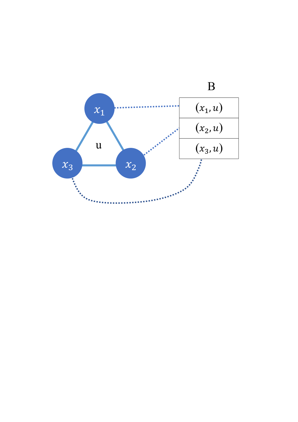
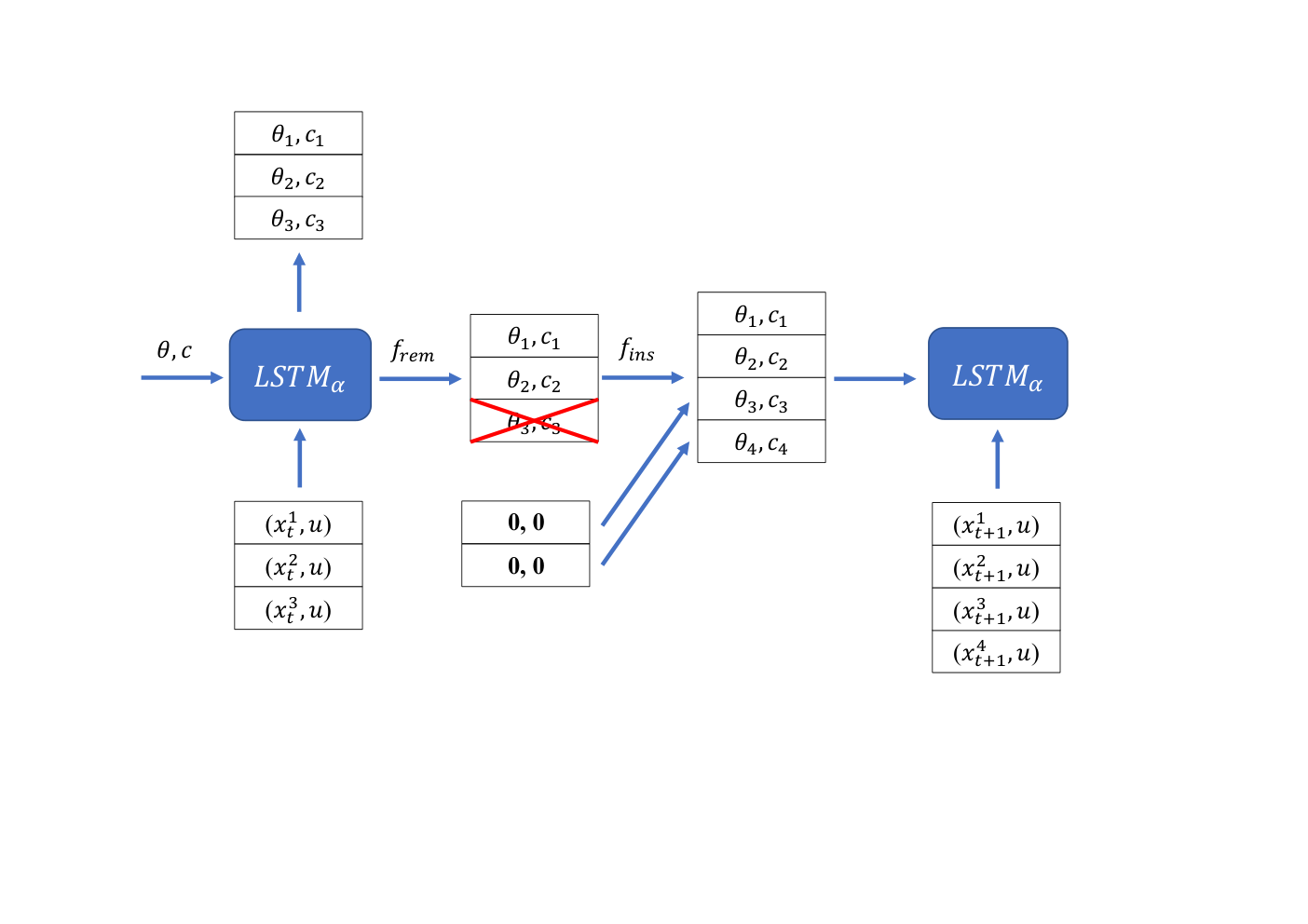
Appendix D Input Preprocessing and Model Architecture for Methods Addressing Partial Observability
This section details the preprocessing steps and latent variable inference model architectures designed for estimating the learner’s optimal action-value function. We structure this section in terms of the different latent variable inference models defined in Section 6.1.
D.1 Particle-based Belief Inference
Input Preprocessing. To preprocess the learner’s observations in partially observable environments, we assume knowledge over the set of agents that exists in the environment, . Based on the learner’s observation, for each agent in we also assume access to their ID, personal features, and visibility in the observation. Finally, the learner also remembers the action which it has executed in the previous timestep .
The aforementioned knowledge is subsequently preprocessed into a set of feature vectors for belief updates. For each , their ID, personal features, and visibility in the observation are concatenated as their personal agent features, . The remaining global information not associated to any agent () is subsequently concatenated to the personal agent features to finally form an observation batch for learning, . This preprocessing step is illustrated in Figure 16.
Joint Action Inference Models. The proposal and target action distribution for joint action inference are implemented as networks with similar architecture. The only difference is that the proposal action distribution includes and as its input. Formally, the input for the proposal network and for the target network are defined as follows:
| (54) |
The network architecture to compute the proposal and target action distribution subsequently evaluates the joint action probability distribution as:
| (55) |
with,
| (56) | ||||
Assuming that and are the parameters of the proposal and target action distribution respectively, our implementation uses separate neural networks for estimating these distributions, such that .
Existence and State Inference Models. As in the case with joint action inference models, input for the proposal and target distributions in existence and state inference is derived from concatenating all the necessary information as defined below:
| (57) |
For existence inference, we assume a unique integer index assigned to each agent in , where the index assigned to is denoted as . Subsequently, both the target and proposal distribution are implemented as a neural network which computes agents’ existence in the following manner:
| (58) |
with,
| (59) | ||||
This autoregressive existence inference technique resembles GraphRNN (You et al. 2018), which is a generative model that generates graphs with varying numbers of nodes in an autoregressive fashion.
For state inference, both the proposal and target distributions are represented as multivariate normal distribution with a diagonal covariance matrix, , which parameters are evaluated by neural networks following this expression:
| (60) | ||||
| (61) |
In our implementation, the target and proposal distribution for teammate existence and state inference are implemented as separate models which parameters are denoted as and respectively.
Type Update Network. We implement the type update network as an LSTM which accounts for agents’ previous types and recently inferred state representation and actions to compute their respective types. The type update process in the type update network is provided in the following expression:
| (62) | ||||
| (63) |
with and being the cell and hidden state that represents the sequence of previously inferred state and type representations. The input to the LSTM model is subsequently defined below:
| (64) |
Observation Likelihood Model. We assume that the observation vector that we reconstruct is the preprocessed data vector, . Since is a collection of continuous vectors, we use a multivariate normal distribution, , which parameters are computed as defined below:
| (65) | ||||
| (66) |
with the input to this model defined as:
| (67) |
D.2 Variational Autoencoder-based Belief Inference
Given the observations from the environment, , we first preprocess them to obtain the vector . This preprocessing step is similar as the one done in particle-based methods which we detail in Appendix D.1. Then, at every timestep, is used as input to the encoder architecture to compute the distribution over latent variables . Furthermore, also acts as the information which will be reconstructed by the decoder. The architecture of the encoder and decoder is provided below.
Encoder Network The encoder network is implemented as an LSTM which receives the learner’s preprocessed observation, , as input. It subsequently produces the mean and covariance matrix for the variational parametric distribution following this expression:
| (68) | ||||
| (69) |
where,
| (70) |
with and being the LSTM’s cell and hidden state that represents the sequence of previous observations.
Decoder Network. Since the role of the decoder is to reconstruct the information observed by the learner, we train the decoder to reconstruct the learner’s observations alongside predicting its observed teammates’ actions. The decoder network subsequently outputs both the likelihood of alongside the likelihood of observed teammates’ actions. Since is a collection of continuous vectors, we compute the likelihood of based on a multivariate normal distribution, , which parameters are computed as defined below:
| (71) | ||||
| (72) |
assuming is sampled from the variational parametric distribution outputted by the learner.
On the other hand, the part of the decoder that predicts the likelihood of teammates’ actions has a similar implementation as the joint action inference model for the particle-based approach in Section D.1. Given , the decoder computes the likelihood of observed agents’ actions using a GNN following this equation:
| (73) |
assuming denotes the set of visible teammates and with,
| (74) | ||||
D.3 Autoencoder-based Inference
Given input data which is obtained in a similar way as the VAE-based inference model, the encoder outputs a representation that is defined as the following:
| (75) |
where,
| (76) |
and and are the cell and hidden states of the LSTM. The interaction data gathered by the learner is then used to train the encoder’s parameters to produce that contains important information regarding the learner’s interaction experience.
The training process utilises a decoder network to produce that is representative of the learner’s interaction experience. The decoder network receives as input and is trained to reconstruct the learner’s current observation alongside predicting the observed teammates’ previous joint actions. Given , the reconstructed observation outputted by the decoder is denoted by:
| (77) |
On the other hand, the part of the decoder that predicts teammates’ joint actions is similar to the action prediction part of the VAE’s decoders defined in Equation 73. Assuming that the parameters of this model is denoted by , the only difference is that this model receives as input rather than .
Appendix E Agent and Joint Action Value Modelling Learning Under Partial Observability
In this section, we describe the loss functions to train GPL’s agent and joint action value modelling components under partial observability. While the details of the loss functions depend on the latent variable inference being used, all loss functions are based on GPL’s optimised loss functions described in Equation 15 and 16. Details of the agent and joint action value modelling losses for each latent variable inference model are provided in the following sections.
E.1 Particle-based Belief Inference
Agent Modelling Loss Function. While other methods use separate models for agent modelling and latent variable inference, the target action distribution estimation model, , is reused for agent modelling when using particle-based belief models. This reuse is motivated by how GPL’s agent modelling process introduced in Section 4.4 aims to estimate the target action distribution in the first place. Therefore, the negative log likelihood loss is computed by assuming . The negative log likelihood loss is then defined as:
| (78) |
where the joint action log likelihood is only evaluated over observed teammates’ joint actions.
Reinforcement Learning Loss Function. We assume that the CG-based model used in action value computation defined in Section 6.3.3 is parameterised by such that . Assuming denotes the set of possible joint actions of unobserved agents, the CG-based joint action value model is then trained to estimate the optimal joint action value function by optimising:
| (79) |
where,
| (80) |
is the estimated joint action value of agents that are visible to the learner at based on the contents of particle . Specifically, is computed via Equation 8 while is evaluated based on Equation 13.
The target value for particle is then defined based on , which is the particle resulting from updating based on and according to Section 6.3.2 excluding the particle sampling step. The target value is then defined as:
| (81) |
with evaluated according to Equation 53. Note that unlike in the RL loss under full observability, we consider the particle weights in the loss computation to allow less likely particles to have higher temporal difference errors.
E.2 Variational Autoencoder-based Belief Inference
Agent Modelling Loss Function. Agent modelling under the VAE-based model is done via the action prediction component of the decoder, which in our description at Section D.2 is parameterised by . This model is chosen for agent modelling since its purpose is also to predict teammates’ joint actions. Assuming , the loss function of this model is defined as:
| (82) |
Reinforcement Learning Loss Function. As in GPL, we define a CG-based model to estimate the joint action values of the learner. Assuming that the parameters of this model is denoted as , this model must be trained to estimate the joint action value given the variational parametric distribution, . Since exactly computing is generally intractable, we use a Monte Carlo approach for training this model. Under this approach, we sample vectors from such that:
| (83) |
The sampled are subsequently used as input to the CG model, which loss function for joint action value modelling is subsequently computed as:
| (84) |
assuming . In Equation 84, the predicted joint action value of observed teammates’ joint actions is defined as:
| (85) |
which is similar to the predicted value under particle-based approaches. Finally, the target value is defined as:
| (86) |
with computed according to Equation 43.
E.3 Autoencoder-based Inference
Agent Modelling Loss Function. Given produced by the encoder, GPL’s agent and joint action model are trained to estimate the learner’s action value function. We use the decoder’s action prediction component for agent modelling since it is also designed to predict teammates’ actions. Assuming , the agent model is subsequently trained to predict observed teammates’ actions by minimising the following loss function:
| (87) |
Reinforcement Learning Loss Function. We train the joint action value model by optimising the temporal difference error defined below:
| (88) |
Given the parameters of the joint action value model , the predicted and target joint action value are evaluated following Equation 85 and 86.
Appendix F Partial observability results
F.1 Baselines
To run the single agent baselines in environments with a changing number of teammates we assign a value of -1 to features associated with inactive agents. In our experiments we can have up to five agents in the environment, so we add these placeholder values to the input to match the size of the input vector when five agents are present. To prevent teammates’ features from always being assigned a placeholder, which could hurt generalisation, we assign agents entering the environment an index number. We use this index to determine the location of their features in the input vector. This index remains the same while an agent is active in the environment.
For DVRL we utilised the code made available by the original authors. We utilised similar hyperparameters as the authors. We used 10 particles, with an action encoding of 16, the dimension is 100, and the dimension is 100. All neural networks utilise a hidden layer size of 100 unless stated. We used RMSProp with , a gradient clipping of 0.5, learning rate , and gamma 0.99. For encoding the set particles into we utilised a fully connected neural network. Actions are encoded by a fully connected neural network with two layers of 64 units. The policy is one fully connected layer whose size is determined by the action space. DVRL uses A2C, with 16 parallel environments, and a 5-step learning.
For PPO we utilised the following hyperparameter: a fully connected network with two hidden layers of 128 neurons each, a learning rate of , a batch size of 64, a number of epochs 10, and a number of steps of 2048.
F.2 Unseen teammates
For the experiments with unseen teammates, we created a set of 8 different reinforcement learning agents all trained with different seeds, which were added to the pool of existing teammates. The policies of the set of unseen teammates were obtained via reinforcement learning, particularly the PPO algorithm. The set of unseen agents is able to observe the full state of the system in order to make decisions. To encode the policies of the unseen teammates we utilised an MLP network with two hidden layers of 128 neurons each, a learning rate of , a batch size of 64, a number of epochs 10, and a number of steps of 2048.
References
- Agarwal et al. (2021) Rishabh Agarwal, Max Schwarzer, Pablo Samuel Castro, Aaron Courville, and Marc G Bellemare. Deep reinforcement learning at the edge of the statistical precipice. Advances in Neural Information Processing Systems, 2021.
- Agmon and Stone (2012) Noa Agmon and Peter Stone. Leading ad hoc agents in joint action settings with multiple teammates. In Proceedings of the 11th International Conference on Autonomous Agents and Multiagent Systems - Volume 1, AAMAS ’12, page 341–348, Richland, SC, 2012. International Foundation for Autonomous Agents and Multiagent Systems. ISBN 0981738117.
- Albrecht and Ramamoorthy (2015) Stefano V. Albrecht and Subramanian Ramamoorthy. Are you doing what I think you are doing? criticising uncertain agent models. In Proceedings of the 31st Conference on Uncertainty in Artificial Intelligence, pages 52–61, 2015.
- Albrecht and Ramamoorthy (2016) Stefano V. Albrecht and Subramanian Ramamoorthy. Exploiting causality for selective belief filtering in dynamic Bayesian networks. Journal of Artificial Intelligence Research, 55:1135–1178, 2016. DOI: 10.1613/jair.5044.
- Albrecht and Ramamoorthy (2017) Stefano V. Albrecht and Subramanian Ramamoorthy. Exploiting causality for selective belief filtering in dynamic bayesian networks. In Proceedings of the 26th International Joint Conference on Artificial Intelligence, IJCAI’17, page 5085–5089. AAAI Press, 2017. ISBN 9780999241103.
- Albrecht and Stone (2017) Stefano V. Albrecht and Peter Stone. Reasoning about hypothetical agent behaviours and their parameters. In Proceedings of the 16th Conference on Autonomous Agents and MultiAgent Systems, AAMAS ’17, page 547–555, Richland, SC, 2017. International Foundation for Autonomous Agents and Multiagent Systems.
- Albrecht and Stone (2018) Stefano V. Albrecht and Peter Stone. Autonomous agents modelling other agents: A comprehensive survey and open problems. Artificial Intelligence, 258:66–95, May 2018. ISSN 00043702. doi: 10.1016/j.artint.2018.01.002.
- Albrecht et al. (2016) Stefano V. Albrecht, Jacob W Crandall, and Subramanian Ramamoorthy. Belief and truth in hypothesised behaviours. Artificial Intelligence, 235:63–94, 2016.
- Albrecht et al. (2023) Stefano V. Albrecht, Filippos Christianos, and Lukas Schäfer. Multi-Agent Reinforcement Learning: Foundations and Modern Approaches. MIT Press, 2023. URL https://www.marl-book.com.
- Arulampalam et al. (2002) M.S. Arulampalam, S. Maskell, N. Gordon, and T. Clapp. A tutorial on particle filters for online nonlinear/non-gaussian bayesian tracking. IEEE Transactions on Signal Processing, 50(2):174–188, 2002. doi: 10.1109/78.978374.
- Barrett et al. (2012) Samuel Barrett, Peter Stone, Sarit Kraus, and Avi Rosenfeld. Learning teammate models for ad hoc teamwork. In AAMAS Adaptive Learning Agents (ALA) Workshop, June 2012.
- Barrett et al. (2014) Samuel Barrett, Noa Agmon, Noam Hazon, Sarit Kraus, and Peter Stone. Communicating with unknown teammates. In ECAI 2014, volume 263 of Frontiers in Artificial Intelligence and Applications, pages 45–50, Prague, Czech Republic, 2014. IOS Press. doi: 10.3233/978-1-61499-419-0-45. Publisher: IOS Press.
- Barrett et al. (2017) Samuel Barrett, Avi Rosenfeld, Sarit Kraus, and Peter Stone. Making friends on the fly: Cooperating with new teammates. Artificial Intelligence, 242:132–171, 2017. ISSN 0004-3702. doi: https://doi.org/10.1016/j.artint.2016.10.005. URL https://www.sciencedirect.com/science/article/pii/S0004370216301266.
- Boehmer et al. (2020) Wendelin Boehmer, Vitaly Kurin, and Shimon Whiteson. Deep coordination graphs. In Proceedings of the 37th International Conference on Machine Learning, ICML 2020, 13-18 July 2020, Virtual Event, volume 119 of Proceedings of Machine Learning Research, pages 980–991. PMLR, 2020.
- Boldrer et al. (2022) Manuel Boldrer, Alessandro Antonucci, Paolo Bevilacqua, Luigi Palopoli, and Daniele Fontanelli. Multi-agent navigation in human-shared environments: A safe and socially-aware approach. Robotics and Autonomous Systems, 149:103979, 2022. ISSN 0921-8890. doi: https://doi.org/10.1016/j.robot.2021.103979.
- Carlucho et al. (2022) Ignacio Carlucho, Arrasy Rahman, William Ard, Elliot Fosong, Corina Barbalata, and Stefano V Albrecht. Cooperative marine operations via ad hoc teams. arXiv preprint arXiv:2207.07498, 2022.
- Chandrasekaran et al. (2016) Muthukumaran Chandrasekaran, Adam Eck, Prashant Doshi, and Leenkiat Soh. Individual planning in open and typed agent systems. In Proceedings of the Thirty-Second Conference on Uncertainty in Artificial Intelligence, UAI’16, pages 82–91, Jersey City, New Jersey, USA, June 2016. AUAI Press. ISBN 978-0-9966431-1-5.
- Coquelin et al. (2009) Pierre-arnaud Coquelin, Romain Deguest, and Rémi Munos. Particle filter-based policy gradient in pomdps. In D. Koller, D. Schuurmans, Y. Bengio, and L. Bottou, editors, Advances in Neural Information Processing Systems, volume 21. Curran Associates, Inc., 2009.
- Do et al. (2019) Kien Do, Truyen Tran, and Svetha Venkatesh. Graph transformation policy network for chemical reaction prediction. In Proceedings of the 25th ACM SIGKDD International Conference on Knowledge Discovery, KDD ’19, page 750–760, New York, NY, USA, 2019. Association for Computing Machinery. ISBN 9781450362016. doi: 10.1145/3292500.3330958.
- Doshi and Gmytrasiewicz (2011) Prashant Doshi and Piotr J. Gmytrasiewicz. A framework for sequential planning in multi-agent settings. CoRR, abs/1109.2135, 2011. URL http://arxiv.org/abs/1109.2135.
- Doucet et al. (2001) Arnaud Doucet, Nando de Freitas, and Neil Gordon. An introduction to sequential monte carlo methods. In Sequential Monte Carlo methods in practice, pages 3–14. Springer, 2001.
- Eck et al. (2020) Adam Eck, Maulik Shah, Prashant Doshi, and Leen-Kiat Soh. Scalable decision-theoretic planning in open and typed multiagent systems. In Proceedings of the AAAI Conference on Artificial Intelligence, volume 34, pages 7127–7134, 2020.
- Foerster et al. (2016) Jakob Foerster, Ioannis Alexandros Assael, Nando De Freitas, and Shimon Whiteson. Learning to communicate with deep multi-agent reinforcement learning. Advances in neural information processing systems, 29, 2016.
- Foerster et al. (2018) Jakob Foerster, Gregory Farquhar, Triantafyllos Afouras, Nantas Nardelli, and Shimon Whiteson. Counterfactual multi-agent policy gradients. In Proceedings of the AAAI Conference on Artificial Intelligence, volume 32, 2018.
- Gogineni et al. (2023) Kailash Gogineni, Peng Wei, Tian Lan, and Guru Venkataramani. Scalability bottlenecks in multi-agent reinforcement learning systems, 2023.
- Gronauer and Diepold (2022) Sven Gronauer and Klaus Diepold. Multi-agent deep reinforcement learning: a survey. Artificial Intelligence Review, 55(2):895–943, Feb 2022. ISSN 1573-7462. doi: 10.1007/s10462-021-09996-w. URL https://doi.org/10.1007/s10462-021-09996-w.
- Grover et al. (2019) Aditya Grover, Aaron Zweig, and Stefano Ermon. Graphite: Iterative generative modeling of graphs. In Kamalika Chaudhuri and Ruslan Salakhutdinov, editors, Proceedings of the 36th International Conference on Machine Learning, volume 97 of Proceedings of Machine Learning Research, pages 2434–2444. PMLR, 09–15 Jun 2019.
- Gu et al. (2021) Pengjie Gu, Mengchen Zhao, Jianye Hao, and Bo An. Online ad hoc teamwork under partial observability. In International Conference on Learning Representations, 2021.
- Guestrin et al. (2002a) Carlos Guestrin, Michail G. Lagoudakis, and Ronald Parr. Coordinated reinforcement learning. In Proceedings of the Nineteenth International Conference on Machine Learning, ICML ’02, page 227–234, San Francisco, CA, USA, 2002a. Morgan Kaufmann Publishers Inc. ISBN 1558608737.
- Guestrin et al. (2002b) Carlos Guestrin, Michail G Lagoudakis, and Ronald Parr. Coordinated reinforcement learning. In Proceedings of the Nineteenth International Conference on Machine Learning, pages 227–234, 2002b.
- Haarnoja et al. (2018) Tuomas Haarnoja, Aurick Zhou, Pieter Abbeel, and Sergey Levine. Soft actor-critic: Off-policy maximum entropy deep reinforcement learning with a stochastic actor. In International Conference on Machine Learning, pages 1861–1870. PMLR, 2018.
- Harsanyi (1967) John C. Harsanyi. Games with incomplete information played by “Bayesian” players, I–III Part I. The basic model. Management Science, 14(3):159–182, November 1967. ISSN 0025-1909, 1526-5501. doi: 10.1287/mnsc.14.3.159.
- Hausknecht and Stone (2015) Matthew Hausknecht and Peter Stone. Deep recurrent q-learning for partially observable mdps. In 2015 aaai fall symposium series, 2015.
- Hoang and Low (2013) Trong Nghia Hoang and Kian Hsiang Low. Interactive pomdp lite: Towards practical planning to predict and exploit intentions for interacting with self-interested agents. arXiv preprint arXiv:1304.5159, 2013.
- Hochreiter and Schmidhuber (1997) Sepp Hochreiter and Jürgen Schmidhuber. Long Short-Term Memory. Neural Computation, 9(8):1735–1780, 11 1997. ISSN 0899-7667. doi: 10.1162/neco.1997.9.8.1735.
- Hu et al. (2020) Hengyuan Hu, Adam Lerer, Alex Peysakhovich, and Jakob Foerster. “Other-play” for zero-shot coordination. In International Conference on Machine Learning, volume 119, pages 4399–4410, 2020.
- Huang et al. (2020) Wenlong Huang, Igor Mordatch, and Deepak Pathak. One policy to control them all: Shared modular policies for agent-agnostic control. In International Conference on Machine Learning, pages 4455–4464. PMLR, 2020.
- Igl et al. (2018) Maximilian Igl, Luisa M. Zintgraf, Tuan Anh Le, Frank Wood, and Shimon Whiteson. Deep variational reinforcement learning for pomdps. In Jennifer G. Dy and Andreas Krause, editors, Proceedings of the 35th International Conference on Machine Learning, ICML 2018, Stockholmsmässan, Stockholm, Sweden, July 10-15, 2018, volume 80 of Proceedings of Machine Learning Research, pages 2122–2131. PMLR, 2018.
- Izadi and Precup (2005) Masoumeh T. Izadi and Doina Precup. Using rewards for belief state updates in partially observable markov decision processes. In Machine Learning: ECML 2005, pages 593–600, Berlin, Heidelberg, 2005. Springer Berlin Heidelberg. ISBN 978-3-540-31692-3.
- Jiang et al. (2019) Jiechuan Jiang, Chen Dun, Tiejun Huang, and Zongqing Lu. Graph convolutional reinforcement learning. In International Conference on Learning Representations, 2019.
- Kingma and Welling (2013) Diederik P Kingma and Max Welling. Auto-encoding variational bayes. arXiv preprint arXiv:1312.6114, 2013.
- Krnjaic et al. (2023) Aleksandar Krnjaic, Raul D. Steleac, Jonathan D. Thomas, Georgios Papoudakis, Lukas Schäfer, Andrew Wing Keung To, Kuan-Ho Lao, Murat Cubuktepe, Matthew Haley, Peter Börsting, and Stefano V. Albrecht. Scalable multi-agent reinforcement learning for warehouse logistics with robotic and human co-workers, 2023.
- Le et al. (2018) Tuan Anh Le, Maximilian Igl, Tom Rainforth, Tom Jin, and Frank Wood. Auto-encoding sequential monte carlo. In International Conference on Learning Representations, 2018.
- Lowe et al. (2017) Ryan Lowe, Yi I Wu, Aviv Tamar, Jean Harb, OpenAI Pieter Abbeel, and Igor Mordatch. Multi-agent actor-critic for mixed cooperative-competitive environments. In Advances in neural information processing systems, pages 6379–6390, 2017.
- Lupu et al. (2021) Andrei Lupu, Brandon Cui, Hengyuan Hu, and Jakob Foerster. Trajectory diversity for zero-shot coordination. In Marina Meila and Tong Zhang, editors, Proceedings of the 38th International Conference on Machine Learning, volume 139 of Proceedings of Machine Learning Research, pages 7204–7213. PMLR, 18–24 Jul 2021. URL https://proceedings.mlr.press/v139/lupu21a.html.
- Macke et al. (2021) William Macke, Reuth Mirsky, and Peter Stone. Expected value of communication for planning in ad hoc teamworks. In Proceedings of the AAAI Conference on Artificial Intelligence, 2021.
- Mirsky et al. (2020) Reuth Mirsky, William Macke, Andy Wang, Harel Yedidsion, and Peter Stone. A penny for your thoughts: The value of communication in ad hoc teamwork. In Christian Bessiere, editor, Proceedings of the Twenty-Ninth International Joint Conference on Artificial Intelligence, IJCAI-20, pages 254–260. International Joint Conferences on Artificial Intelligence Organization, 7 2020. doi: 10.24963/ijcai.2020/36.
- Mirsky et al. (2022) Reuth Mirsky, Ignacio Carlucho, Arrasy Rahman, Elliot Fosong, William Macke, Mohan Sridharan, Peter Stone, and Stefano V. Albrecht. A survey of ad hoc teamwork research. European Conference on Multi-Agent Systems (EUMAS), 2022.
- Mnih et al. (2015) Volodymyr Mnih, Koray Kavukcuoglu, David Silver, Andrei A Rusu, Joel Veness, Marc G Bellemare, Alex Graves, Martin Riedmiller, Andreas K Fidjeland, Georg Ostrovski, et al. Human-level control through deep reinforcement learning. nature, 518(7540):529–533, 2015.
- Mnih et al. (2016) Volodymyr Mnih, Adria Puigdomenech Badia, Mehdi Mirza, Alex Graves, Timothy Lillicrap, Tim Harley, David Silver, and Koray Kavukcuoglu. Asynchronous methods for deep reinforcement learning. In International conference on machine learning, pages 1928–1937, 2016.
- Morad et al. (2023) Steven Morad, Ryan Kortvelesy, Matteo Bettini, Stephan Liwicki, and Amanda Prorok. POPGym: Benchmarking partially observable reinforcement learning. In The Eleventh International Conference on Learning Representations, 2023. URL https://openreview.net/forum?id=chDrutUTs0K.
- Murphy and Russell (2001) Kevin Murphy and Stuart Russell. Rao-blackwellised particle filtering for dynamic bayesian networks. In Sequential Monte Carlo methods in practice, pages 499–515. Springer, 2001.
- Naderializadeh et al. (2020) Navid Naderializadeh, Fan Hung, Sean Soleyman, and Deepak Khosla. Graph convolutional value decomposition in multi-agent reinforcement learning. ArXiv, abs/2010.04740, 2020.
- Papoudakis et al. (2021) Georgios Papoudakis, Filippos Christianos, and Stefano V. Albrecht. Agent modelling under partial observability for deep reinforcement learning. In NeurIPS, 2021.
- Rahman et al. (2023a) Arrasy Rahman, Jiaxun Cui, and Peter Stone. Minimum coverage sets for training robust ad hoc teamwork agents. arXiv preprint arXiv:2308.09595, 2023a.
- Rahman et al. (2023b) Arrasy Rahman, Elliot Fosong, Ignacio Carlucho, and Stefano V. Albrecht. Generating teammates for training robust ad hoc teamwork agents via best-response diversity. Transactions on Machine Learning Research (TMLR), 2023b. ISSN 2835-8856. URL https://openreview.net/forum?id=l5BzfQhROl.
- Rahman et al. (2021) Muhammad A Rahman, Niklas Hopner, Filippos Christianos, and Stefano V Albrecht. Towards open ad hoc teamwork using graph-based policy learning. In International Conference on Machine Learning, pages 8776–8786. PMLR, 2021.
- Rashid et al. (2018) Tabish Rashid, Mikayel Samvelyan, Christian Schroeder, Gregory Farquhar, Jakob Foerster, and Shimon Whiteson. Qmix: Monotonic value function factorisation for deep multi-agent reinforcement learning. In International conference on machine learning, pages 4295–4304. PMLR, 2018.
- Ravula et al. (2019) Manish Ravula, Shani Alkoby, and Peter Stone. Ad hoc teamwork with behavior switching agents. In Proceedings of the 28th International Joint Conference on Artificial Intelligence, pages 550–556, Macau, China, August 2019. International Joint Conferences on Artificial Intelligence Organization. ISBN 978-0-9992411-4-1. doi: 10.24963/ijcai.2019/78.
- Ribeiro et al. (2022) João G. Ribeiro, Cassandro Martinho, Alberto Sardinha, and Francisco S. Melo. Assisting unknown teammates in unknown tasks: Ad hoc teamwork under partial observability. arXiv preprint arXiv:2201.03538, 2022.
- Roesch et al. (2020) Martin Roesch, Christian Linder, Roland Zimmermann, Andreas Rudolf, Andrea Hohmann, and Gunther Reinhart. Smart grid for industry using multi-agent reinforcement learning. Applied Sciences, 10(19), 2020. ISSN 2076-3417. doi: 10.3390/app10196900.
- Rumelhart et al. (1985) David E Rumelhart, Geoffrey E Hinton, and Ronald J Williams. Learning internal representations by error propagation. Technical report, California Univ San Diego La Jolla Inst for Cognitive Science, 1985.
- Schulman et al. (2017) John Schulman, Filip Wolski, Prafulla Dhariwal, Alec Radford, and Oleg Klimov. Proximal policy optimization algorithms, 2017.
- Shapley (1953) L. S. Shapley. Stochastic games. Proceedings of the National Academy of Sciences, 39(10):1095–1100, October 1953. ISSN 0027-8424, 1091-6490. doi: 10.1073/pnas.39.10.1095.
- Singh et al. (2021) Gautam Singh, Skand Peri, Junghyun Kim, Hyunseok Kim, and Sungjin Ahn. Structured world belief for reinforcement learning in pomdp. In Marina Meila and Tong Zhang, editors, Proceedings of the 38th International Conference on Machine Learning, volume 139 of Proceedings of Machine Learning Research, pages 9744–9755. PMLR, 18–24 Jul 2021.
- Stone and Kraus (2010) Peter Stone and Sarit Kraus. To teach or not to teach? decision making under uncertainty in ad hoc teams. In The Ninth International Conference on Autonomous Agents and Multiagent Systems (AAMAS). International Foundation for Autonomous Agents and Multiagent Systems, May 2010.
- Stone et al. (2010) Peter Stone, Gal A. Kaminka, Sarit Kraus, and Jeffrey S. Rosenschein. Ad hoc autonomous agent teams: Collaboration without pre-coordination. In Proceedings of the Twenty-Fourth Conference on Artificial Intelligence, July 2010.
- Sunehag et al. (2017) Peter Sunehag, Guy Lever, Audrunas Gruslys, Wojciech Marian Czarnecki, Vinicius Zambaldi, Max Jaderberg, Marc Lanctot, Nicolas Sonnerat, Joel Z Leibo, Karl Tuyls, et al. Value-decomposition networks for cooperative multi-agent learning. arXiv preprint arXiv:1706.05296, 2017.
- Tacchetti et al. (2018) Andrea Tacchetti, H. Francis Song, Pedro A. M. Mediano, Vinicius Zambaldi, Neil C. Rabinowitz, Thore Graepel, Matthew Botvinick, and Peter W. Battaglia. Relational forward models for multi-agent learning. In International Conference on Learning Representations, New Orleans, USA, September 2018. OpenReview.net. arXiv: 1809.11044.
- Tacchetti et al. (2019) Andrea Tacchetti, H. Francis Song, Pedro A. M. Mediano, Vinícius Flores Zambaldi, János Kramár, Neil C. Rabinowitz, Thore Graepel, Matthew Botvinick, and Peter W. Battaglia. Relational forward models for multi-agent learning. In 7th International Conference on Learning Representations, 2019.
- Vezhnevets et al. (2020) Alexander Vezhnevets, Yuhuai Wu, Maria Eckstein, Rémi Leblond, and Joel Z. Leibo. OPtions as REsponses: Grounding behavioural hierarchies in multi-agent reinforcement learning. In International Conference on Machine Learning, pages 9733–9742, 2020.
- Wang et al. (2019) Minjie Wang, Lingfan Yu, Da Zheng, Quan Gan, Yu Gai, Zihao Ye, Mufei Li, Jinjing Zhou, Qi Huang, Chao Ma, Ziyue Huang, Qipeng Guo, Hao Zhang, Haibin Lin, Junbo Zhao, Jinyang Li, Alexander J Smola, and Zheng Zhang. Deep graph library: Towards efficient and scalable deep learning on graphs. ICLR Workshop on Representation Learning on Graphs and Manifolds, 2019.
- Watkins and Dayan (1992) Christopher JCH Watkins and Peter Dayan. Q-learning. Machine learning, 8(3-4):279–292, 1992.
- Wierstra et al. (2007) Daan Wierstra, Alexander Foerster, Jan Peters, and Jürgen Schmidhuber. Solving deep memory pomdps with recurrent policy gradients. In Joaquim Marques de Sá, Luís A. Alexandre, Włodzisław Duch, and Danilo Mandic, editors, Artificial Neural Networks – ICANN 2007, pages 697–706, Berlin, Heidelberg, 2007. Springer Berlin Heidelberg. ISBN 978-3-540-74690-4.
- Wu et al. (2019) Zonghan Wu, Shirui Pan, Fengwen Chen, Guodong Long, Chengqi Zhang, and Philip S. Yu. A comprehensive survey on graph neural networks. IEEE Transactions on Neural Networks and Learning Systems, 32:4–24, 2019.
- Xie et al. (2021) Annie Xie, Dylan Losey, Ryan Tolsma, Chelsea Finn, and Dorsa Sadigh. Learning latent representations to influence multi-agent interaction. In Conference on robot learning, pages 575–588. PMLR, 2021.
- You et al. (2018) Jiaxuan You, Rex Ying, Xiang Ren, William Hamilton, and Jure Leskovec. Graphrnn: Generating realistic graphs with deep auto-regressive models. In International conference on machine learning, pages 5708–5717. PMLR, 2018.
- Zheng et al. (2020) Chuanpan Zheng, Xiaoliang Fan, Cheng Wang, and Jianzhong Qi. GMAN: A graph multi-attention network for traffic prediction. In The Thirty-Fourth AAAI Conference on Artificial Intelligence, AAAI 2020, The Thirty-Second Innovative Applications of Artificial Intelligence Conference, IAAI 2020, The Tenth AAAI Symposium on Educational Advances in Artificial Intelligence, EAAI 2020, New York, NY, USA, February 7-12, 2020, pages 1234–1241. AAAI Press, 2020.
- Zhou et al. (2019) Ming Zhou, Yong Chen, Ying Wen, Yaodong Yang, Yufeng Su, Weinan Zhang, Dell Zhang, and Jun Wang. Factorized q-learning for large-scale multi-agent systems. In Proceedings of the First International Conference on Distributed Artificial Intelligence, pages 1–7, 2019.
- Zhou et al. (2021) Weigui Jair Zhou, Budhitama Subagdja, Ah-Hwee Tan, and Darren Wee-Sze Ong. Hierarchical control of multi-agent reinforcement learning team in real-time strategy (rts) games. Expert Systems with Applications, 186:115707, 2021. ISSN 0957-4174. doi: https://doi.org/10.1016/j.eswa.2021.115707.