Intrinsic Dimension for Large-Scale Geometric Learning

Maximilian Stubbemann stubbemann@cs.uni-kassel.de Affiliation: Knowledge & Data Engineering Group, University of Kassel, Kassel, Germany Tom Hanika tom.hanika@cs.uni-kassel.de Affiliation: Knowledge & Data Engineering Group, University of Kassel, Kassel, Germany Friedrich Martin Schneider martin.schneider@math.tu-freiberg.de Affiliation: Institute of Discrete Mathematics and Algebra, TU Bergakademie Freiberg, Freiberg, Germany

Abstract

The concept of dimension is essential to grasp the complexity of data. A naive approach to determine the dimension of a dataset is based on the number of attributes. More sophisticated methods derive a notion of intrinsic dimension (ID) that employs more complex feature functions, e.g., distances between data points. Yet, many of these approaches are based on empirical observations, cannot cope with the geometric character of contemporary datasets, and do lack an axiomatic foundation. A different approach was proposed by V. Pestov, who links the intrinsic dimension axiomatically to the mathematical concentration of measure phenomenon. First methods to compute this and related notions for ID were computationally intractable for large-scale real-world datasets. In the present work, we derive a computationally feasible method for determining said axiomatic ID functions. Moreover, we demonstrate how the geometric properties of complex data are accounted for in our modeling. In particular, we propose a principle way to incorporate neighborhood information, as in graph data, into the ID. This allows for new insights into common graph learning procedures, which we illustrate by experiments on the Open Graph Benchmark.

1 Introduction

Contemporary real-world datasets employed in artificial intelligence are often large in size and comprised of complex structures, which distinguishes them from Euclidean data. To consider these properties appropriately is a challenging task for procedures that analyze or learn from said data. Moreover, with increasing complexity of real-world data, the necessity arises to quantify to which extent this data suffer from the curse of dimensionality. The common approach for estimating the dimension curse of a particular dataset is through the notion of intrinsic dimension (ID) (Bac & Zinovyev 2020; Granata & Carnevale 2016; Pestov 2007). There exists a variety of work on how to estimate the ID of datasets (Facco et al. 2017; Levina & Bickel 2004; Costa et al. 2005; Gomtsyan et al. 2019; Bac & Zinovyev 2020). Most approaches to quantify the ID are based on distances between data points, assuming the data to be Euclidean. A multitude of works base their modeling on the manifold hypothesis (Cloninger & Klock 2021; Gomtsyan et al. 2019), which assumes that the observed data is embedded in a manifold of low dimension (compared to the number of data attributes). The ID then is an approximation of the dimension of this manifold. Pestov 2000 proposed a different concept of intrinsic dimension by linking it to the mathematical concentration of measure phenomenon. His modeling is based on a thorough axiomatic approach (Pestov 2007; Pestov 2008; Pestov 2010) which resulted in a novel class of intrinsic dimension functions. In contrast to the manifold hypothesis, Pestov’s ID functions measure to which extent a dataset is affected by the curse of dimensionality, i.e., to which extent the complexity of the dataset hinders the discrimination of data points. Yet, to compute said ID functions is an intractable computational endeavor. This limitation was overcome in principle by an adaptation to geometric datasets (Hanika et al. 2022). However, two limitations persisted: First, the computational effort was found to remain quadratic in the number of data points, which is insufficient for datasets of contemporary size; second, it is unclear how to account for complex structure, such as in graph data.

With this in mind, we propose in the present work a default approach for computing the intrinsic dimension of geometric data, such as graph data, as used in graph neural networks. To do this, we revisit the computation of the ID based on distance functions (Hanika et al. 2022) and overcome, in particular, the inherent computational limitations in the works by Pestov 2007 and Hanika et al. 2022. In detail, we derive a novel approximation formula and present an algorithm for its computation. This allows us to compute ID bounds for datasets that are magnitudes larger than in earlier works. That equipped with, we establish a natural approach to compute the ID of graph data.

We subsequently apply our method to seven real-world datasets and relate the obtained results to the observed performances of classification procedures. Thus, we demonstrate the practical computability of our approach. In addition, we study the extent to which the intrinsic dimension reveals insights into the performance of particularly classes of Graph Neural Networks. Our code is publicly available on GitHub.¹¹ 1 https://github.com/mstubbemann/ID4GeoL

2 Related Work

In numerous works, the intrinsic dimension is estimated using the pairwise distances between data points (Chávez et al. 2001; Grassberger & Procaccia 2004). More sophisticated approaches use distances to nearest neighbors (Facco et al. 2017; Levina & Bickel 2004; Costa et al. 2005; Gomtsyan et al. 2019). All these works have in common, that they assume the data to be Euclidean and that they favor local properties.

Recent work has drawn different connections between intrinsic dimension (ID) and modern learning theory. For example, Cloninger & Klock 2021 show that functions of the form $f(x)=g(\phi(x))$ , where $\phi$ maps into a manifold of lower dimension, can be approximated by neural networks. On the other hand, Wojtowytsch & E 2020 prove that modern artificial neural networks suffer from the curse of dimensionality in the sense that gradient training on high dimensional data may converge insufficiently. Additional to these theoretical results, there is an increasing interest of empirically estimating the ID of contemporary learning architectures. Li et al. 2018 study the ID of neural networks by replacing high dimensional parameter vectors with lower dimensional ones. Their approach results in a non-deterministic ID. More recent works studied ID in the realm of geometric data and their standard architectures. Ansuini et al. 2019 investigate the ID for convolutional neural networks (CNN). In detail, they are interested to which extent the ID changes at different hidden layers and how this is related to the overall classification performance. Another work (Pope et al. 2020) associates an ID to popular benchmark image datasets. These two works on ID estimators do solely rely on the metric information of the data and do not consider any geometric structure of image data.

Our approach allows to incorporate such underlying geometric structures while incorporating the mathematical phenomenon of measure concentration (Gromov & Milman 1983; Milman 1988; Milman 2010). Linking this phenomenon to the occurrence of the dimension curse was done by Pestov (Pestov 2000; Pestov 2007; Pestov 2008; Pestov 2010). He based his considerations on a thorough axiomatic approach using techniques from metric-measure spaces. The resulting ID functions unfortunately turn out to be practically incomputable. In contrast, Bac & Zinovyev 2020 investigate computationally feasible ID estimators that are related to the concentration phenomenon. Yet, their results elude a comparable axiomatic foundation. Our modeling for the ID of large and geometric data is based on Hanika et al. 2022. We build on their axiomatization and derive a computationally feasible method for the intrinsic dimension of large-scale geometric datasets.

3 Intrinsic Dimension

Since our work is based on the formalization from Hanika et al. 2022, we shortly revisit their modeling and recapitulate the most important structures. Based on this, we derive and prove an explicit formula to compute the ID for the special case of finite geometric datasets. This first result is essential for Section 4.

Let $\mathcal{D}=(X,F,\mu)$ , where $X$ is a set and $F\subseteq{\mathbb{R}}^{X}$ is a set of functions from $X$ to $\mathbb{R}$ , in the following called feature functions. We require that $\sup_{x,y\in X}d_{F}(x,y)<\infty$ , where $d_{F}(x,y)\coloneqq\sup_{f\in F}|f(x)-f(y)|$ . If $(X,d_{F})$ constitutes a complete and separable metric space such that $\mu$ is a Borel probability measure on $(X,d_{F})$ , we call $\mathcal{D}$ a geometric dataset (GD). The aforementioned properties are satisfied when it holds that $0<|X|,|F|<\infty$ and that $F$ can discriminate all data points, i.e., $d_{F}(x,y)>0$ for all $x,y\in X$ with $x\neq y$ .

Two geometric datasets $\mathcal{D}_{1}\coloneqq(X_{1},F_{1},\mu_{1}),\mathcal{D}_{2}\coloneqq(X_{2},F_{2},\mu_{2})$ are isomorphic if there exists a bijection $\phi:X_{1}\to X_{2}$ such that $\overline{F_{2}}\circ\phi=\overline{F_{1}}$ and $\phi_{*}(\mu_{1})=\mu_{2}$ , where $\phi_{*}(\mu_{1})(B)\coloneqq\mu_{1}(\phi^{-1}(B))$ is the push-forward measure and the closures are taken with respect to point-wise convergence. From this point on we identify a geometric dataset with its isomorphism class. The triple $(\{\emptyset\},\mathbb{R},\nu_{\{\emptyset\}})$ represents the trivial geometric dataset.

Pestov 2007 defines the curse of dimensionality as “[…] a name given to the situation where all or some of the important features of a dataset sharply concentrate near their median (or mean) values and thus become non-discriminating. In such cases, X is perceived as intrinsically high-dimensional.” Thus, the ID estimator aims to compute to which extent the features allow to discriminate different data points. For a specific feature $f\in F$ , Hanika et al. 2022 therefore defines the partial diameter of $f$ with regard to a specific $\alpha\in(0,1)$ such that it displays to which extent $f$ can discriminate subsets with minimal measure $1-\alpha$ , i.e., via

\partdiam(f_{*}(\nu),1{-}\alpha)=\inf\{\diam(B)\penalty\ |\penalty\ B\subseteq\mathbb{R}\text{ Borel, }\nu(f^{-1}(B))\geq 1-\alpha\},

where $\diam(B)\coloneqq\sup_{a,b\in B}|a-b|$ . The observable diameter with respect to $\alpha$ then defines to which extent $F$ can discriminate points with minimum measure 1- $\alpha$ by being defined as the supremum of the partial diameter of all $f\in F$ , i.e, $\obsdiam(\mathcal{D},-\alpha)\coloneqq\sup_{f\in F}\partdiam(f_{*}(\mu),1-\alpha)$ . To observe the discriminability for different minimal measures $\alpha$ , the discriminability $\Delta(\mathcal{D})$ of $\mathcal{D}$ and the intrinsic dimension $\partial(\mathcal{D})$ are defined via

\partial(\mathcal{D})\coloneqq\frac{1}{\Delta(\mathcal{D})^{2}},\quad\text{where}\quad\Delta(\mathcal{D})\coloneqq\int_{0}^{1}\obsdiam(\mathcal{D},-\alpha)\penalty\ d\alpha.

(1)

In other words, lower values of intrinsic dimensionality correspond to geometric datasets with points that can be better discriminated by the given set of feature functions. This intrinsic dimension function is, in principle, applicable to a broad variety of geometric data, such as metric data, graphs or images. This applicability arises from the possibility to choose suitable feature functions which reflect the underlying data structure. The appropriate choice of feature functions is part of Section 5. Furthermore, the ID $\partial(\mathcal{D})=\frac{1}{\Delta(\mathcal{D})^{2}}$ respects the formal axiomatization (Hanika et al. 2022) for ID functions, informally:

•

Axiom of concentration: A sequence of geometric datasets converges against the constant dataset (meaning having no chance to separate data points!), if and only if their IDs diverge against infinity.
•

Axiom of feature antitonicity: If dataset $\mathcal{D}_{1}$ has more feature functions then $\mathcal{D}_{0}$ (i.e. having potentially more information to separate data points), it should have a lower intrinsic dimension.
•

Axiom of continuity: If a sequence of geometric datasets converge against a specific geometric dataset, the sequence of the IDs should converge against the ID of the limit geometric dataset.
•

Axiom of geometric order of divergence: If a sequence of geometric datasets converges against the constant dataset, its IDs should diverge against infinity with the same order as $\frac{1}{\Delta(\mathcal{(}D))^{2}}$ does.

3.1 Intrinsic Dimension of Finite Data

We want to apply Equation 1 to real-world data. In the following, let $\mathcal{D}=(X,F,\nu)$ such that $0<|X|<\infty$ and $0<|F|<\infty$ and let $\nu$ be the normalized counting measure on $X$ , i.e., $\nu(M)\coloneqq\frac{|M|}{|X|}$ for $M\subseteq X$ . In this case, it is possible to compute the partial diameter and Equation 1, as we show in the following. Let $\alpha\in(0,1)$ and let $c_{\alpha}\coloneqq\lceil|X|(1-\alpha)\rceil$ . The following arguments were already hinted in previous work (Hanika et al. 2022), yet not formally discussed or proven.

Lemma 3.1.

For $f\in F$ it holds that

\partdiam(f_{*}(\nu),1-\alpha)=\min_{|M|=c_{\alpha}}\max_{x,y\in M}|f(x)-f(y)|.

Proof.

It holds that

	$\displaystyle\partdiam(f_{*}(\nu),1{-}\alpha)$	$\displaystyle=\inf\{\diam(B)\penalty\ \|\penalty\ B\subseteq\mathbb{R}\text{ Borel, }\nu(f^{-1}(B))\geq 1-\alpha\}$
		$\displaystyle=\inf\{\diam(B)\penalty\ \|\penalty\ B\subseteq\mathbb{R}\text{ Borel,}\|\{x\in X\penalty\ \|\penalty\ f(x)\in B\}\|{\geq}c_{\alpha}\}.$

We have to show that

\displaystyle\begin{split}\inf\{\diam(B)\penalty\ |\penalty\ B\subseteq\mathbb{R}\text{ Borel, }|\{x\in X\penalty\ |\penalty\ f(x)\in B\}|\geq c_{\alpha}\}=\\ \min\{\max_{x,y\in M}|f(x)-f(y)|\penalty\ |\penalty\ M\subseteq X,|M|\geq c_{\alpha}\}.\end{split}

(2)

“ $\leq:$ ” We show that $\{\diam(B)\penalty\ |\penalty\ B\subseteq\mathbb{R}\text{ Borel, }|\{x\in X\penalty\ |\penalty\ f(x)\in B\}|\geq c_{\alpha}\}\supseteq\{\max_{x,y\in M}|f(x)-f(y)|\penalty\ |\penalty\ M\subseteq X,|M|\geq c_{\alpha}\}$ . Let $z\coloneqq\max_{x,y\in M}|f(x)-f(y)|$ such that $M\subseteq X$ with $|M|\geq c_{\alpha}$ . Without loss of generality we assume that

\forall x\in X:(\exists m_{1},m_{2}\in M:f(m_{1})\leq f(x)\leq f(m_{2})\implies x\in M).

Let $b\coloneqq\max_{x\in M}f(x)$ , $a\coloneqq\min_{x\in M}f(x)$ , then $M=\{x\in X\penalty\ |\penalty\ f(x)\in[a,b]\}$ . Hence, $z=b-a\in\{\diam(B)|B\subseteq\mathbb{R}\text{ Borel,}|\{x\in X|f(x)\in B\}|\geq c_{\alpha}\}$ .

“ $\geq:$ ” Let $B\subseteq\mathbb{R}$ be Borel with $|\{x\in X\penalty\ |\penalty\ f(x)\in B\}|\geq c_{\alpha}$ . Furthermore, let $M\coloneqq\{x\in X\penalty\ |\penalty\ f(x)\in B\}$ . It holds that $\diam(B)=\sup_{x,y\in B}|x-y|\geq\max_{x,y\in M}|f(x)-f(y)|$ because of the choice of $M$ . As $B$ was chosen arbitrarily, it follows “ $\geq$ ”.

Finally, we need that

\min\{\max_{x,y\in M}|f(x)-f(y)|\penalty\ |\penalty\ |M|\geq c_{\alpha}\}=\min\{\max_{x,y\in M}|f(x)-f(y)|\penalty\ |\penalty\ |M|=c_{\alpha}\}.

“ $\leq$ ” follows directly from the fact that $\{\max_{x,y\in M}|f(x)-f(y)|\penalty\ |\penalty\ |M|\geq c_{\alpha}\}\supseteq\{\max_{x,y\in M}|f(x)-f(y)|\penalty\ |\penalty\ |M|=c_{\alpha}\}$ . “ $\geq$ ” follows from the fact that for every $|M|\geq c_{\alpha}$ and for every $N\subseteq M$ with $|N|=c_{\alpha}$ the following equation holds: $\sup_{x,y\in M}|f(x)-f(y)|\geq\sup_{x,y\in N}|f(x)-f(y)|$ . ∎

This lemma allows for a more tractable formula for the computation of the partial diameter of a finite GD. That in turn enables the following theorem.

Theorem 3.2.

It holds that

\Delta(\mathcal{D})=\frac{1}{|X|}\sum_{k=2}^{|X|}\max_{f\in F}\mathop{\min_{M\subseteq X}}_{|M|=k}\max_{x,y\in M}|f(x)-f(y)|.

(3)

Proof.

Let $g:(0,1)\to\mathbb{R},\alpha\mapsto\max_{f\in F}\min_{M\subseteq X,|M|=c_{\alpha}}\max_{x,y\in M}|f(x)-f(y)|$ . Because of Lemma 3.1 we know that $\Delta({\mathcal{D}})=\int_{0}^{1}g(\alpha)\penalty\ d\alpha$ . The function $g$ is a step function which can be expressed for each $\alpha\in(0,1)$ via

g(\alpha)=\sum_{k=1}^{|X|}\mathbbm{1}_{\left(\frac{|X|-k}{|X|},\frac{|X|+1-k}{|X|}\right)}(\alpha)\max_{f\in F}\mathop{\min_{M\subseteq X}}_{|M|=k}\max_{x,y\in M}|f(x)-f(y)|

almost everywhere. Hence, Equation 3 follows from the definition of the Lebesgue-Integral with the fact that $\min_{M\subseteq X,|M|=1}\max_{x,y\in M}|f(x)-f(y)|=0$ . ∎

In general, the addition of features should lower the ID since we have additional information that helps to discriminate the data. However, there are certain features that are not helping to further discriminate data points. These are for example:

1.

Constant features. This is due to the fact that for a constant feature $f$ it always holds for all $M\subseteq X$ that $\max_{x,y\in M}|f(x)-f(y)|=0$ .
2.

Permutations of already existing features. Let $\tilde{f}:X\to\mathbb{R}$ have the form $\tilde{f}=f\circ\pi$ with $\pi:X\to X$ being a permutation on $X$ . Then there exist for all $M\subseteq X$ with $|M|=k$ a set $N\subseteq X$ with $|N|=k$ and $\max_{x,y\in M}|f(x)-f(y)|=\max_{x,y\in N}|\tilde{f}(x)-\tilde{f}(y)|$ and vice versa.

Thus, we have the following Lemma.

Lemma 3.3.

Let $\mathcal{D}=(X,F,\mu)$ be a finite geometric dataset. Furthermore, let $\hat{F}$ be a set of constant functions $X\to\mathbb{R}$ and let $\tilde{F}$ be a set of functions $X\to\mathbb{R}$ such that there exist for each $\tilde{f}\in\tilde{F}$ a $f\in F$ and a permutation $\pi:X\to X$ with $\tilde{f}=f\circ\pi$ . Let $\mathcal{E}\coloneqq(X,F\cup\hat{F}\cup\tilde{F},\mu)$ . Then it holds that $\partial(D)=\partial(E)$ .

3.2 Computing the Intrinsic Dimension of Finite Data

In this section we will propose an algorithm for computing the ID based on Equation 3. For this, given a finite geometric dataset $\mathcal{D}$ , we use the shortened notations $\phi_{k,f}(\mathcal{D})\coloneqq\min_{M\subseteq X,|M|=k}\max_{x,y\in M}|f(x)-f(y)|$ and $\phi_{k}(\mathcal{D})\coloneqq\max_{f\in F}\phi_{k,f}(\mathcal{D})$ . Then, Equation 3 can be written as

\Delta(\mathcal{D})=\frac{1}{|X|}\sum_{k=2}^{|X|}\phi_{k}(\mathcal{D})=\frac{1}{|X|}\sum_{k=2}^{|X|}\max_{f\in F}\phi_{k,f}(\mathcal{D}).

(4)

The straightforward computation of Equation 4 is hindered by the task to iterate through all subsets $M\subseteq X$ of size $k$ . This yields an exponential complexity with respect to $|X|$ for computing $\Delta(\mathcal{D})$ . We can overcome this towards a quadratic computational complexity in $|X|$ using the following concept.

Definition 3.4.

(Feature Sequence) For a feature $f\in F$ let $l_{f,\mathcal{D}}\in\mathbb{R}^{|X|}$ be the increasing sequence of all values $f(x)$ for $x\in X$ . We call $l_{f,\mathcal{D}}=(l_{1}^{f,\mathcal{D}},\dots,l_{|X|}^{f,\mathcal{D}})$ the feature sequence of $f$ .

Using these sequences, the following lemma allows us to efficiently compute $\phi_{k,f}(\mathcal{D})$ .

Lemma 3.5.

For $k\in\{2,\dotsc,|X|\},f\in F$ and $l_{f,\mathcal{D}}$ , it holds that

\phi_{k,f}(\mathcal{D})=\min\{l_{k+j}^{f,\mathcal{D}}-l_{1+j}^{f,\mathcal{D}}\penalty\ |\penalty\ j\in\{0,\dots,|X|-k\}\}.

Proof.

For all $j\in\{0,\dots,|X|-k\}$ there exist $M\subseteq X$ with $|M|=k$ and $l_{k+j}^{f,\mathcal{D}}-l_{1+j}^{f,\mathcal{D}}=\max_{x,y\in M}|f(x)-f(y)|$ . Thus, it is sufficient to show $\phi_{k,f}(\mathcal{D})\in\{l_{k+j}^{f,\mathcal{D}}-l_{1+j}^{f,\mathcal{D}}\penalty\ |\penalty\ j\in\{0,\dots,|X|-k\}\}$ . Choose $M\subseteq X$ with $|M|=k$ such that $\phi_{k,f}(\mathcal{D})=\max_{x,y\in M}|f(x)-f(y)|$ holds. Furthermore, let $l^{M}\coloneqq(l_{1}^{M},\dots,l_{k}^{M})$ be the increasing sequence of values $f(m)$ for $m\in M$ and let $j\in\{0,\dots,|X|-k\}$ such that $l_{1}^{M}=l_{1+j}^{f,\mathcal{D}}$ . Since $l^{M}$ is an ordered sequence of which each element is also an element of the ordered sequence $l_{f,\mathcal{D}}$ , it holds that $l_{k}^{M}\geq l_{k+j}^{f,\mathcal{D}}$ and thus $l_{k}^{M}-l_{1}^{M}\geq l^{f,\mathcal{D}}_{j+k}-l_{j+1}^{f,\mathcal{D}}$ . There is an $N\subseteq X$ with size $k$ such that $\max_{x,y\in N}|f(x)-f(y)|=l_{k+j}^{f,\mathcal{D}}-l_{k+1}^{f,\mathcal{D}}$ . Since $M\subseteq X$ is of size $k$ such that $\max_{x,y\in M}|f(x)-f(y)|$ is minimal, it follows $l_{k}^{M}-l_{1}^{M}=\max_{x,y\in M}|f(x)-f(y)|\leq\max_{x,y\in N}|f(x)-f(y)|=l_{k+j}^{f,\mathcal{D}}-l_{k+1}^{f,\mathcal{D}}$ , hence $\phi_{k,f}(\mathcal{D})=\max_{x,y\in M}|f(x)-f(y)|=l_{k}^{M}-l_{1}^{M}=l_{k+j}^{f,\mathcal{D}}-l_{k+1}^{f,\mathcal{D}}$ . ∎

Input : Finite geometric dataset

\mathcal{D}=(X,\mu,F)

Output :

\Delta(\mathcal{D})

forall $f$ in $F$ do 1

Compute feature sequence

l_{f,\mathcal{D}}

\Delta(\mathcal{D})=0

forall $k$ in $\{2,\dots,|X|\}$ do 2

forall $f$ in $F$ do 3

\phi_{k,f}(\mathcal{D})=\min_{j\in\{0,\dots,|X|-k\}}l_{k+j}^{f,\mathcal{D}}-l_{1+j}^{f,\mathcal{D}}

\Delta(\mathcal{D})+=\max_{f\in F}\phi_{k,f}(\mathcal{D})

\Delta(\mathcal{D})=\frac{1}{|X|}\Delta(\mathcal{D})

return

\Delta(\mathcal{D})

Algorithm 1 The pseudocode to compute

\Delta(\mathcal{D})

for a finite geometric dataset

\mathcal{D}=(X,\mu,F)

To sum up, Lemma 3.5 enables the efficient computation of $\phi_{k,f}(\mathcal{D})$ via a sliding window, i.e., by using only pairs of elements $(l_{1+j}^{f,\mathcal{D}},l_{k+j}^{f,\mathcal{D}})$ . The algorithm based on this is shown in Algorithm 1. We want to provide a brief description of the most relevant steps. In Line 4 we iterate through the sizes of $X$ by setting $k\in\{2,\dots,|X|\}$ in order to compute $\phi_{k}(\mathcal{D})$ in Lines 6 and 7. For this we also need to iterate over all $f\in F$ (Line 5) to compute the necessary values of $\phi_{k,f}(\mathcal{D})$ in Line 6. For a given $f\in F,k\in\{1,\dots,|X|\}$ , Line 6 consumes $|X|-k+1$ subtraction operations. Assuming that computing feature values can be done in constant time, the runtime for computing $\Delta(\mathcal{D})$ from the feature sequences is $\mathcal{O}(|F|\sum_{k=2}^{|X|}|X|-k+1)=\mathcal{O}(|F|\sum_{k=1}^{|X|-1}k)=\mathcal{O}(|F|\,|X|^{2})$ . The creation of all feature sequences requires $\mathcal{O}(|F||X|\log(|X|))$ computations , which is negligible compared to the aforementioned complexity. Thus, Algorithm 1 has quadratic complexity with respect to $|X|$ . Therefore, Algorithm 1 is a straightforward and easy to implement solution for the computation of the ID. However, its quadratic runtime is obstructive for the application in large-scale data problems, which raises the necessity for a modification. We will present such a modification in the following section.

4 Intrinsic Dimension for Large-Scale Data

In order to speed up the computation of the ID we modify Algorithm 1 with regard to the accuracy of the result. Hence, we settle for an efficiently computable approximation of the ID. To give an overview over the necessary steps, we will

1.

approximate the ID by replacing $\{2,\dots,|X|\}$ in Line 4 of Algorithm 1 with a smaller subset $S\subseteq\{2,\dots,|X|\}$ , which we represent by $S\coloneqq\{s_{1},\dots,s_{l}\}$ . For all $k\not\in S$ , we will use $\{\phi_{s_{1}}(\mathcal{D}),\dots,\phi_{s_{l}}(\mathcal{D})\}$ to estimate $\phi_{k}(\mathcal{D})$ . This will eventually lead to two approximations of the ID, an underestimation and an overestimation.
2.

compare the upper and lower approximation to provide an error bound of these approximations with respect to the exact ID. This error bound can be computed without knowing the exact ID.
3.

argue how, the computation of the exact ID can be sped up with the help of knowledge about $\phi_{s_{i}}(\mathcal{D})$ for all $s_{i}\in S$ . For this, we will in particular show that we can replace for all $k\in\{2,\dots,|X|\}\setminus M$ the set $F$ with a subset $\hat{F}$ , see Line 5-6 of Algorithm 1.
4.

derive a formula which estimates the amount of computation cost which is saved by using only subsets of $F$ for the computation of the ID. This information can be used to estimate and decide whether the exact computation of the ID is computational feasible for a specific dataset.

The ensuing algorithm is shown in Algorithm 2. The underlying theory that justifies it is presented in the following. This theory will be based on the monotonicity of $i\mapsto\phi_{i,f}(\mathcal{D})$ .

Theorem 4.1.

For $m>n\geq 2$ and $f\in F$ the following statements hold.

1.

$\phi_{m,f}(\mathcal{D})\geq\phi_{n,f}(\mathcal{D})$ ,
2.

$\phi_{m}(\mathcal{D})\geq\phi_{n}(\mathcal{D})$ .

Proof.

The second inequality follows directly from the first one. Since per definition $\phi_{m,f}(\mathcal{D})=\min_{M\subseteq X,|M|=m}\max_{x,y\in M}|f(x)-f(y)|$ and also $\phi_{n,f}(\mathcal{D})=\min_{N\subseteq X,|N|=n}\max_{x,y\in N}|f(x)-f(y)|$ , we need to show that for each $M\subseteq X$ with $|M|=m$ there exist $N\subseteq X$ with $|N|=n$ and $\max_{x,y\in M}|f(x)-f(y)|\geq\max_{x,y\in N}|f(x)-f(y)|$ . It is sufficient to show that for $n=m-1$ . Choose $x_{1},x_{2}\in M$ such that $\max_{x,y\in M}|f(x)-f(y)|=|f(x_{1})-f(x_{2})|$ . As $|M|>2$ we find $x_{3}\in M\setminus\{x_{1},x_{2}\}$ . Let $N\coloneqq M\setminus\{x_{3}\}$ . It holds that $\max_{x,y\in M}|f(x)-f(y)|=|f(x_{1})-f(x_{2})|=\max_{x,y\in N}|f(x)-f(y)|$ . ∎

Input : Finite GD

\mathcal{D}=(X,\mu,F)

, support sequence

s=(2=s_{1},\dots,s_{l}=|X|)

, exact (Boolean)

Output :

\Delta_{s,-}(\mathcal{D}),\Delta_{s,+}(\mathcal{D}),\Delta(\mathcal{D})

forall $f$ in $F$ do 1

Compute feature sequence

l_{f,\mathcal{D}}

\Delta(\mathcal{D})=0

s_{0}=1

\phi_{s_{0}}(\mathcal{D})=0

forall $i$ in $\{1,\dots,l\}$ do // Iterate over support sequence indices 2

forall $f$ in $F$ do 3

\phi_{s_{i},f}(\mathcal{D})=\min_{j\in\{0,\dots,|X|-s_{i}\}}l_{s_{i}+j}^{f,\mathcal{D}}-l_{1+j}^{f,\mathcal{D}}

// Compute

\phi_{s_{i},f}(\mathcal{D})

with Lemma 3.5

\phi_{s_{i}}(\mathcal{D})=\max_{f\in F}\phi_{s_{i},f}(\mathcal{D})

F_{s_{i-1}}=\{f\in F\penalty\ |\penalty\ \phi_{s_{i},f}(\mathcal{D})>\phi_{s_{i-1}}(\mathcal{D})\}

// Compute

F_{s_{i-1}}

for Lemma 4.7

\Delta(\mathcal{D})+=\phi_{s_{i}}(\mathcal{D})

\Delta_{s,-}(\mathcal{D})=\frac{1}{|X|}(\Delta(\mathcal{D})+\sum_{i=1}^{l-1}\sum_{s_{i}<j<s_{i+1}}\phi_{s_{i}}(\mathcal{D}))

// Compute lower ID from Definition 4.2

\Delta_{s,+}(\mathcal{D})=\frac{1}{|X|}(\Delta(\mathcal{D})+\sum_{i=1}^{l-1}\sum_{s_{i}<j<s_{i+1}}\phi_{s_{i+1}}(\mathcal{D}))

// Compute upper ID from Definition 4.2

// Approximation finished. Continue with exact computation, if desired.

if exact then 4

forall $i$ in $\{1,\dots l\}$ do 5

forall $s_{i}<j<s_{i+1}$ do // Iterate through all indices between two support elements 6

forall $f$ in $F_{s_{i}}$ do // Only iterate through

F_{s_{i}}

because of Lemma 4.7 7

\phi_{s_{i},f}(\mathcal{D})=\min_{j\in\{0,\dots,|X|-s_{i}\}}l_{s_{i}+j}^{f,\mathcal{D}}-l_{1+j}^{f,\mathcal{D}}

\phi_{j}(\mathcal{D})=\max(\{\phi_{j,f}(\mathcal{D})\penalty\ |\penalty\ f\in F_{i}\}\cup\{\phi_{s_{i}}\})

// Use Lemma 4.7

\Delta(\mathcal{D})+=\phi_{j}(\mathcal{D})

\Delta(\mathcal{D})=\frac{1}{|X|}\Delta(\mathcal{D})

return

\Delta_{s,-}(\mathcal{D}),\Delta_{s,+}(\mathcal{D}),\Delta(\mathcal{D})

return

\Delta_{s,-}(\mathcal{D}),\Delta_{s,+}(\mathcal{D})

Algorithm 2 The pseudocode to compute

\Delta_{s,-}(\mathcal{D}),\Delta_{s,+}(\mathcal{D}),\Delta(\mathcal{D})

for a finite GD

\mathcal{D}=(X,\mu,F)

4.1 Computing Intrinsic Dimension via Support Sequences

Equipped with Theorem 4.1, we can bound $\Delta(\mathcal{D})$ and thus the intrinsic dimension through computing $\phi_{s_{i}}$ for a few $2=s_{1}<s_{2}\dots<s_{l}=|X|$ .

Definition 4.2.

(Support Sequences and Upper / Lower ID) Let $s=(2=s_{1},\dots,s_{l-1},s_{l}=|X|)$ be a strictly increasing and finite sequence of natural numbers. We call $s$ a support sequence of $\mathcal{D}$ . We additionally define

\displaystyle\begin{split}\Delta_{s,-}(\mathcal{D})&\coloneqq\frac{1}{|X|}\left(\sum_{i=1}^{l}\phi_{s_{i}}(\mathcal{D})+\sum_{i=1}^{l-1}\sum_{s_{i}<j<s_{i+1}}\phi_{s_{i}}(\mathcal{D})\right),\\ \Delta_{s,+}(\mathcal{D})&\coloneqq\frac{1}{|X|}\left(\sum_{i=1}^{l}\phi_{s_{i}}(\mathcal{D})+\sum_{i=1}^{l-1}\sum_{s_{i}<j<s_{i+1}}\phi_{s_{i+1}}(\mathcal{D})\right)\end{split}

(5)

and call accordingly $\partial_{s,-}(\mathcal{D})\coloneqq\frac{1}{\Delta_{s,+}(\mathcal{D})^{2}}$ the lower intrinsic dimension of $\mathcal{D}$ and $\partial_{s,+}(\mathcal{D})\coloneqq\frac{1}{\Delta_{s,-}(\mathcal{D})^{2}}$ the upper intrinsic dimension of $D$ .

The governing idea is for $i\in\{1,\dots,l\}$ and $j$ with $s_{i}<j<s_{i+1}$ to substitute $\phi_{j}(\mathcal{D})$ with $\phi_{s_{i}}(\mathcal{D})$ or $\phi_{s_{i+1}}(\mathcal{D})$ . With Theorem 4.1 this results in lower and upper bounds for $\Delta(\mathcal{D})$ and thus for the intrinsic ID. By comparing upper and lower bounds, we can approximate the ID and estimate the approximation error.

Corollary 4.3.

For support sequences $s$ holds $\Delta_{s,-}(\mathcal{D})\leq\Delta(\mathcal{D})\leq\Delta_{s,+}(\mathcal{D})$ and $\partial_{s,-}(\mathcal{D})\leq\partial(\mathcal{D})\leq\partial_{s,+}(\mathcal{D})$ .

Definition 4.4 (Approximation Error).

For a support sequence $s$ the (relative) approximation error of $\partial(\mathcal{D})$ with respect to $s$ is given by

\E(s,\mathcal{D})\coloneqq\frac{\partial_{s,+}(\mathcal{D})-\partial_{s,-}(\mathcal{D})}{\partial_{s,-}(\mathcal{D})}.

With the computation of the upper and lower ID it is possible to bound the error with respect to the ID $\partial(\mathcal{D})$ . The following corollary can be deduced from Corollary 4.3 and Definition 4.4.

Corollary 4.5.

For a support sequence $s$ the following statements hold.

1.

$\max\{\frac{\partial_{s,+}(\mathcal{D})-\partial(\mathcal{D})}{\partial(\mathcal{D})},\frac{\partial(\mathcal{D})-\partial_{s,-}(\mathcal{D})}{\partial_{s,-}(\mathcal{D})}\},\leq\E(s,\mathcal{D})$ ,
2.

$\max\{|\partial_{s,+}(\mathcal{D})-\partial(\mathcal{D})|,|\partial(\mathcal{D})-\partial_{s,-}(\mathcal{D})|\}\leq|\partial_{s,+}(\mathcal{D})-\partial_{s,-}(\mathcal{D})|$ .

If the error of the approximation of a specific support sequence is not sufficient, further elements can be added to the support sequence. Directly from Equation 5 follows the following corollary.

Corollary 4.6.

Let $s=(2=s_{1},\dots,s_{l}=|X|)$ be a support sequence and let $\hat{s}=(s_{1},\dots,s_{i},p,s_{i+1},\dots,s_{l})$ with a support sequence with an additional element $p$ . Then it holds that

	$\displaystyle\Delta(\mathcal{D})_{\hat{s},-}$	$\displaystyle=\Delta(\mathcal{D})_{s,-}+\frac{\sum_{p\leq j<s_{i+1}}\left((\phi_{p}(\mathcal{D}))-\phi_{s_{i}}(\mathcal{D})\right)}{\|X\|},$
	$\displaystyle\Delta(\mathcal{D})_{\hat{s},+}$	$\displaystyle=\Delta(\mathcal{D})_{s,+}+\frac{\sum_{s_{i}<j\leq p}\left((\phi_{p}(\mathcal{D}))-\phi_{s_{i+1}}(\mathcal{D})\right)}{\|X\|}.$

For a given support sequence $s$ , Corollary 4.5 gives us an upper bound for the error when $\partial_{s,+}(\mathcal{D})$ or $\partial_{s,-}(\mathcal{D})$ are used to approximate $\partial(\mathcal{D})$ without knowing $\partial(\mathcal{D})$ . Hence, we can compute (a lower bound) for the accuracy when approximating the ID with Definition 4.4. As we can see in Section 5.1, Section 5.4 and Section 6, comparable small support sequences lead to sufficient approximations. Support sequences can also be used to shorten the computation of the exact intrinsic dimension as the following lemma shows.

Lemma 4.7.

Let $s=(2=s_{1},\dots,s_{l}=|X|)$ be a support sequence. Furthermore, let $i\in\{1,\dots,l-1\}$ and let $j\in\mathbb{N}$ with $s_{i}<j<s_{i+1}$ . Let $F_{s_{i}}\coloneqq\{f\in F\penalty\ |\penalty\ \phi_{s_{i+1},f}(\mathcal{D})>\phi_{s_{i}}(\mathcal{D})\}$ . Then it holds that

\phi_{j}(\mathcal{D})=\max(\{\phi_{j,f}(\mathcal{D})\penalty\ |\penalty\ f\in F_{s_{i}}\}\cup\{\phi_{s_{i}}(\mathcal{D})\}).

Proof.

“ $\geq$ ” follows from Theorem 4.1 and the definition of $\phi_{j}(\mathcal{D})$ . “ $\leq$ ” holds because for $f\in F\setminus F_{s_{i}}$ it holds that $\phi_{j,f}(\mathcal{D})\leq\phi_{s_{i+1},f}(\mathcal{D})$ , due to Theorem 4.1, and $\phi_{s_{i+1},f}(\mathcal{D})\leq\phi_{s_{i}}(\mathcal{D})$ , due to the construction of $F_{s_{i}}$ . ∎

Hence, given a specific $j$ , it is possible to compute $\phi_{j}(\mathcal{D})$ using a subset of $F$ . Based on the particular GD $\mathcal{D}$ , this fact can considerably speed up the computation of the ID of $\mathcal{D}$ , as we will see in Section 5.

An algorithm to approximate and compute the ID through support sequences is depicted in Algorithm 2. This algorithm takes as input a GD $\mathcal{D}$ and a chosen support sequence $s$ . A reasonable choice for support sequences is discussed in Section 5.1. The output is $\Delta_{s,-}(\mathcal{D}),\Delta_{s,+}(\mathcal{D})$ , and $\Delta(\mathcal{D})$ , if desired (Line 14). In Line 2, all feature sequences are computed. In Line 6 to Line 11, $\phi_{s_{i}}(\mathcal{D})$ and $F_{s_{i-1}}$ , as defined in Lemma 4.7, are computed. From Line 1 to Line 13, the feature sequences and the lower and upper ID are computed. If desired, the exact computation is done in Line 15 to Line 21. Here, we iterate for all support elements (Line 15) through all “gaps” between them (Line 16) and compute $\phi_{j}(\mathcal{D})$ using Lemma 4.7 (Line 17 to Line 19).

4.2 Estimating Computational Costs

Let $s=(s_{1},\dots,s_{l})$ be a support sequence. After the computation of $F_{s_{1}},\dots,F_{s_{l-1}},$ we can estimate how much computation steps we can avoid in order to compute $\partial(\mathcal{D})$ with Algorithm 2 compared to Algorithm 1. Together with the error function $E(s)$ , this estimation can help us to decide if it is desirable to compute the exact value $\partial(\mathcal{D})$ or leave it at $\partial_{s,-}(\mathcal{D})$ and $\partial_{s,+}(\mathcal{D})$ . This is done in the following manner. For a specific $f\in F$ , Lemma 3.5 shows that the computation of $\phi_{k,f}(\mathcal{D})$ requires $|X|-k+1$ different subtractions and to keep the minimum value. Hence, the cost for computing $\Delta(\mathcal{D})$ and therefore $\partial(\mathcal{D})$ via Algorithm 1 can be estimated via $\mathcal{O}(|F|\sum_{k=2}^{|X|}(|X|-k+1))=\mathcal{O}(|F|\sum_{k=1}^{|X|-1}k)=\mathcal{O}(|F|(\frac{|X|^{2}-|X|}{2}))$ . However, if we use Algorithm 2, we solely have the cost to compute $\phi_{s_{i}}$ . For all values $j$ with $s_{i}<j<s_{i+1}$ , our cost estimation is $|F_{s_{i}}|(|X|-j+1)$ . Hence, for a given support sequence $s=(s_{1},\dots,s_{l})$ , we can estimate how many computations are saved using the following notions.

We address the naive computation costs for computing the ID of a GD with

\costs(\mathcal{D})\coloneqq|F|(\frac{|X|^{2}-|X|}{2}).

In contrast, for a support sequence $s=(s_{1},\dots,s_{l})$ of $\mathcal{D}$ , the computation costs are

\costs_{s}(\mathcal{D})\coloneqq(|F|\sum_{k=1}^{l}|X|-s_{k}+1)+\sum_{k=1}^{l-1}|F_{s_{k}}|\sum_{s_{k}<j<s_{k+1}}|X|-j+1.

(6)

Hence, the saved costs of $s$ are

\scosts_{s}(\mathcal{D})\coloneqq 1-\frac{\costs_{s}(\mathcal{D})}{\costs(\mathcal{D})}.

Once we have computed $\phi_{s_{i}}(\mathcal{D})$ and $F_{i}$ , depending on the saved costs, we can decide to discard the support sequence or to continue further computations with it. Furthermore, using the error estimation, we can decide to compute the exact ID or to settle with the approximation.

5 Intrinsic Dimension of Graph Data

Table 1: Statistics of all datasets used in this work.

	Nodes	Edges	Attributes
PubMed	$19,717$	$88,648$	$500$
Cora	$2,708$	$10,556$	$1,433$
CiteSeer	$3,327$	$9,104$	$3,703$
ogbn-arxiv	$169,343$	$1,166,243$	$128$
ogbn-products	$2,449,029$	$61,859,140$	$100$
ogbn-mag	$1,939,743$	$21,111,007$	$128$
ogbn-papers100M	$111,059,956$	$1,615,685,872$	$128$

Figure 1: Example of an

k

-hop geometric dataset with

k=1

. Given are a graph and an attribute matrix

X

. Then, the normalized adjacency matrix

\hat{A}

and then

\hat{A}X

are computed. The feature set

F

consists of the coordinate projections of

X

and

\hat{A}X

. In the figure, every column after “

F=

” represents one

f\in F

. Note, that in this example the normalization factor

\frac{1}{d_{\max}}

1

Graph data is of major interest in the realm of geometric learning and beyond. In the following, a graph dataset $D=(\mathcal{X},G)$ consists of an undirected, unweighted graph $G=(V,E)$ , where $V=\{v_{1},\dots,v_{n}\}$ is a finite set of vertices, $E\subseteq\binom{V}{2}$ and $\mathcal{X}\in\mathbb{R}^{n\times d}$ is a $d$ -dimensional attribute matrix. The row-vector $\mathcal{X}_{i}=(\mathcal{X}_{i,1},\dots,\mathcal{X}_{i,d})$ is called the attribute vector of $v_{i}$ .

Learning from such data is often done via graph neural networks. The idea is to extend common multi-layer perceptrons by a so called neighborhood aggregation, where internal representations of graph neighbors are combined at specific layers. In earlier works, neighborhood aggregation is done at multiple layers (Kipf & Welling 2017; Hamilton et al. 2017; Velickovic et al. 2018). Due to scalability, recent approaches perform multiple iterations of neighborhood aggregation as a preprocessing step and then use the aggregated features as combined input (Rossi et al. 2020; Sun & Wu 2021; Zhang et al. 2021). To be more specific, the employed networks use inputs of the form

(\mathcal{X},\hat{A}\mathcal{X},\hat{A}^{2}\mathcal{X}\dots,\hat{A}^{k}X),

(7)

where $\hat{A}$ is a transition matrix that is derived from the graph structure. The most common choice for such a matrix is the normalized adjacency matrix, i.e., $\hat{A}_{i,j}=(\sqrt{\deg(v_{j})\deg(v_{i})})^{-1}$ if $v_{j}\in N(v_{i})$ and $\hat{A}_{i,j}=0$ else. Here, $N(v_{i})\coloneqq\{v_{j}\in V\penalty\ |\penalty\ \{v_{i},v_{j}\}\in E\}\cup\{v_{i}\}$ is the set of neighbors of $v_{i}$ and $\deg(v_{i})\coloneqq|N(v_{i})|$ is the node degree of $v_{i}$ . The feature set of the following geometric dataset corresponds to the input in Equation 7.

Definition 5.1.

Let $k\in\mathbb{N}$ and $\hat{A}$ be the normalized adjacency matrix of a graph dataset $D$ . Furthermore, let $d_{\max}\coloneqq\max_{j\in\{1,\dots,d\}}\max_{i,k\in\{1,\dots,n\}}|\mathcal{X}_{i,j}-\mathcal{X}_{k,j}|$ . We call the set

F_{D,k}\coloneqq\{v_{i}\mapsto\frac{1}{d_{\max}}(\hat{A}^{m}\mathcal{X})_{i,j}\penalty\ |\penalty\ m\in\{0,\dots,k\},j\in\{1,\dots,d\}\}

the $k$ -hop feature functions of $D$ . Let $\nu$ be the normalized counting measure on $V$ . If there exist for each $v_{i},v_{k}\in V$ with $v_{i}\neq v_{j}$ elements $m\in\{0,\dots,k\},j\in\{1,\dots,d\}$ such that $\frac{1}{d_{\max}}(\hat{A}^{m}\mathcal{X})_{i,j}\neq\frac{1}{d_{\max}}(\hat{A}^{m}\mathcal{X})_{k,j}$ , then $\mathcal{D}_{k}=(V,F_{D,k},\nu)$ is a GD. We call it the $k$ -hop geometric dataset of $D$ .

Basic statistics of all seven graph datasets considered in the following sections are depicted in Table 1. The statistics for Cora, PubMed and CiteSeer were taken from PyTorch Geometric ²² 2 https://pytorch-geometric.readthedocs.io/en/latest/modules/datasets.html#torch_geometric.datasets.Planetoid. The statistics of the OGB datasets were taken from the Open Graph Benchmark. ³³ 3 https://ogb.stanford.edu/docs/nodeprop An example of a $k$ -hop geometric dataset is depicted in Figure 1. It is well-known that the normalized adjacency matrix $\hat{A}\in\mathbb{R}^{n\times n}$ of a graph has a spectral radius of 1. As $\hat{A}$ is symmetric, this yields $\|\hat{A}x-\hat{A}y\|\leq\|x-y\|$ for $x,y\in\mathbb{R}^{n}$ . The significance of this property is for the respective computations, however, limited, since it primarily leads to insights of the behavior of the columns of $\mathcal{X}$ under multiplication with powers of $\hat{A}$ . In contrast, the attribute vectors of the vertices are represented via the rows. Moreover, we may point out that we are not considering the Euclidean distances between attribute vectors, but differences between coordinate values. Thus, the spectral radius of $\hat{A}$ does not provide direct insights into $F_{D,k}$ .

5.1 Choosing Support Sequences

Refer to caption — Figure 2: Errors and saved costs for approximating and computing the intrinsic dimensionality for $2-hop$ geometric datasets with different lengths of the support sequence.

Algorithm 2 relies on a proper choice for a support sequence $s$ . To choose $s$ , two properties have to be considered. Namely, the length of the support sequence and the spacing of the elements. Regarding the second point, we decided to use log-scale spacing. To get such a support sequence for a geometric dataset $\mathcal{D}=(X,F,\mu)$ , we first choose a geometric sequence $\hat{s}=(s_{1},\dots s_{l})$ of length $l$ from $|X|$ to $2$ . We derive the final support sequence $s$ from $s^{\prime}=(\lfloor|X|+2-s_{1}\rfloor,\dots,\lfloor|X|+2-s_{l}\rfloor)$ by removing duplicated elements.

In the following, we study the error and the saved costs for different lengths $l$ of the support sequence. Here, for a geometric dataset, we investigate how $\E(s,\mathcal{D})$ and $\scosts(s)$ vary for $s$ chosen with $l\in\{\lfloor 0.001*|X|\rfloor,\lfloor 0.002*|X|\rfloor,\dots,\lfloor 0.05*|X|\rfloor\}$ . Here, if $l=\lfloor r*|X|\rfloor$ , we call $r\in\mathbb{R}$ the relative support size of the resulting support sequence $s$ . We experiment with common benchmark datasets, namely ogbn-arxiv, ogbn-mag and ogbn-products from the Open Graph Benchmark (Hu et al. 2020; Hu et al. 2021). Since for ogbn-mag only a subset of vertices is equipped with attribute vectors, we generate the missing vectors via metapath2vec (Dong et al. 2017). For all datasets, we consider the $2$ -hop geometric dataset. The results are depicted in Figure 2.

5.1.1 Results

For all datasets, low errors and high saved costs can be reached with a remarkably short support sequence. With relative support sizes of under $0.015$ all datasets are approximated with an accuracy of over $99\%$ . Furthermore, the saved costs for sequences with comparable relative support sizes is over $0.98$ . It stands out, that for the larger datasets ogbn-mag and ogbn-products, shorter sequences (relative to the size of the dataset) lead to lower errors and higher saved costs then for ogbn-arxiv. Our results further indicate, that a relative support size between $0.01$ and $0.02$ is a reasonable range for maximizing the saved costs. For longer support sequences, the saved cost decrease while the error does not change dramatically, at least for the $2$ -hop geometric datasets of ogbn-mag and ogbn-products. Note, that longer support sequence do not always lead to a higher amount of saved costs. For longer support sequences $s$ the costs of computing $\phi_{k}(\mathcal{D})$ for $k\not\in s$ decreases. However, the costs of computing $\phi_{s_{i}}(\mathcal{D})$ for all elements $s_{i}\in s$ increase.

5.2 Neighborhood Aggregation and Intrinsic Dimension

Table 2: Intrinsic dimension and performances on classification tasks. In the upper table, we display IDs for all

k

-hop geometric datasets for

k\in\{0,\dots,5\}

. In the middle table, we display the ID estimated by the MLE baseline. In the lower table we display mean and standard derivations for test accuracy of a standard SIGN model on the classification tasks which belongs to the dataset.

	$0$	$1$	$2$	$3$	$4$	$5$
PubMed	$2542.3425$	$2336.6611$	$2077.5821$	$2077.0953$	$2077.0886$	$2077.0848$
Cora	$6.2523$	$3.8324$	$3.6689$	$3.6627$	$3.6624$	$3.6623$
CiteSeer	$22.3337$	$11.3166$	$10.2347$	$9.8134$	$9.5491$	$9.3795$
ogbn-arxiv	$83.9160$	$31.4731$	$31.4731$	$31.4730$	$30.7370$	$30.3767$
ogbn-products	$1,169,323.2496$	$1,169,044.4736$	$1,169,044.2216$	$1,169,044.2216$	$1,169,044.2216$	$1,169,044.2216$
ogbn-mag	$2,311.3509$	$2,284.0290$	$2,284.0290$	$2,284.0290$	$2,284.0290$	$2,284.0290$

	$0$	$1$	$2$	$3$	$4$	$5$
PubMed	$24.4623$	$24.7303$	$23.3924$	$22.2779$	$21.3495$	$20.5642$
Cora	$30.6049$	$28.1785$	$19.9316$	$10.8186$	$9.2970$	$8.6155$
CiteSeer	$58.9593$	$26.5031$	$16.5556$	$12.0495$	$9.3171$	$7.9572$
ogbn-arxiv	$16.2948$	$19.8571$	$18.9068$	$18.2265$	$17.4905$	$16.9325$
ogbn-products	$2.8694$	$4.7542$	$4.7950$	$4.7659$	$4.6943$	$4.6687$
ogbn-mag	$30.7024$	$33.2848$	$31.5140$	$30.4844$	$29.9080$	$29.5956$

	$0$	$1$	$2$	$3$	$4$	$5$
PubMed	$.6850\pm.0145$	. $7191\pm.0123$	$.7378\pm.0362$	. $7565\pm.0165$	$.7615\pm.0160$	$.7571\pm.0234$
Cora	$.5329\pm.0120$	$.7223\pm.0117$	$.7766\pm.0045$	$.7870\pm.0076$	$.7917\pm.0084$	$.7951\pm.0047$
CiteSeer	$.4975\pm.0075$	$.6165\pm.0160$	$.6530\pm.0101$	$.6677\pm.0074$	$.6695\pm.0085$	$.6734\pm.0080$
ogbn-arxiv	$.5341\pm.0090$	$.6572\pm.0052$	$.6903\pm.0056$	$.6917\pm.0074$	$.6901\pm.0083$	$.6890\pm.0051$
ogbn-products	$.5969\pm.0016$	$.7204\pm.0017$	$.7590\pm.0017$	$.7660\pm.0014$	$.7678\pm.0022$	$.7687\pm.0019$
ogbn-mag	$.2712\pm.0020$	$.3635\pm.0029$	$.3879\pm.0030$	$.3959\pm.0029$	$.3983\pm.0050$	$.4012\pm.0040$

We study how the choice of $k$ affects the intrinsic dimension value of the $k$ -hop geometric dataset. For this, we compute the intrinsic dimension for $k\in\{0,1,\dots,5\}$ for six datasets: the three datasets mentioned above and PubMed, Cora and CiteSeer (Yang et al. 2016), which we retrieved from PyTorch Geometric (Fey & Lenssen 2019). Furthermore, we train GNNs which use the feature functions of $k$ -hop geometric datasets as information for training and inference. This allows us to discover connections between the ID of specific datasets with respect to the considered feature functions and the performance of classifiers, which rely on these feature functions. For this, we train SIGN models (Rossi et al. 2020) for $k\in\{0,\dots,5\}$ . Implementation details and parameter choices can be found in Section A.1.

5.2.1 Baseline Estimator

To investigate to which extent our ID function surpasses established ID estimators with respect to estimating the discriminability of a dataset, we also compute all ID values with the Maximum Likelihood Estimator (MLE) (Levina & Bickel 2004). This estimator is commonly used in the realm of deep learning (Pope et al. 2020; Ma et al. 2018a; Ma et al. 2018b). For our experiments, we use the corrected version proposed by MacKay & Ghahramani 2005. Note, that the MLE is only applicable to datasets $\mathcal{X}\in\mathbb{R}^{n\times d}$ and is thus not able to respect the neighborhood aggregated feature functions. Hence, we incorporate the neighborhood information of a $k$ -hop dataset by concatenating feature vectors with the neighborhood aggregated feature vectors. Due to performance reasons, only subsets of the data points are considered for ogbn-mag and ogbn-products. More details to our usage of the MLE are discussed in Section A.2.

5.2.2 Results

We find that one iteration of neighborhood aggregation always leads to a huge drop of the ID when using our ID function. However, consecutive iterations only lead to a small decrease. For the datasets from OGB, some iterations lead to no drop of the ID dimension at all. For ogbn-mag, only the first iteration significantly decreases the ID, for ogbn-products, only the first two iterations are relevant for decreasing the ID. It stands out, that for ogbn-arxiv, the second and third iteration lead to no significant decrease, but the fourth and fifth do. The results for PubMed stand out. Here, the second iteration of neighborhood aggregation leads to a comparable decrease as the first one.

Considering the classification performances, the first iteration is again the key factor, leading to a significant increase in accuracy. As for the ID, the PubMed dataset behaves differently than the other datasets: the second iteration of neighborhood aggregation leads to a comparable increase in accuracy as the first.

The MLE ID behaves different. Here, no pattern of the first iteration of aggregation being the key for decreasing the data complexity is observed. For some datasets, the first rounds of feature aggregation may even increase the intrinsic dimension. To sum up, our results indicate that our ID is a better indicator for classification performance then the MLE ID.

5.3 Synthetic Data

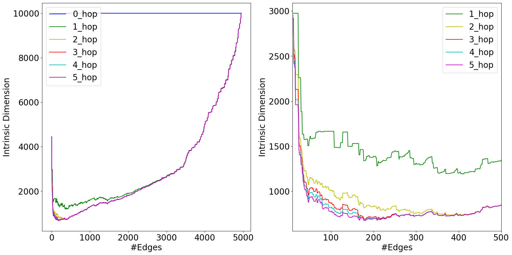
To get further insights into the behavior of our ID notion, we now consider $k-$ hop geometric dataset for one-hot encoded graph data, i.e., $\mathcal{D}=(\mathcal{X},(V,E))$ , with $\mathcal{X}=\mathbb{I}_{|V|}$ where $\mathbb{I}_{|V|}$ is the $|V|$ -dimensional identity matrix. We consider the case of $V=\{1,\dots,100\}$ and determine the ID for $k\in\{0,\dots,5\}$ for increasing edge sizes. To do so, we place the $4950$ possible edges in a random order and add them step by step and compute the ID notions for the $k-$ hop geometric dataset. The results can be found in Figure 3.

5.3.1 Results

The $0-$ hop geometric dataset has an ID which does not depend on the amount of edges. This is not surprising since it does not incorporate any graph information. For all other $k$ values, the ID first sharply decreases and then increases. This indicates that the addition of neighborhood aggregation is particularly useful for graphs of moderate density. Here, the addition of additional rounds of aggregation beyond the first one can further lower the ID. For higher edge sizes, the ID difference between different $k$ values vanishes.

5.4 Approximation of Intrinsic Dimension on Large-Scale Data

To demonstrate the feasibility of our approach, we use it to approximate the ID of the well known, large-scale ogbn-mag-papers100M dataset. For this, we construct the support sequence as in Section 5.1 with $l=100.000$ . The results are depicted in Table 3. On our Xeon Gold System with $16$ cores, approximating the ID of a $k$ -hop geometric dataset build from ogbn-mag-papers100M is possible within a few hours. While the ID drops for every iteration of neighborhood aggregation, the decrease becomes smaller. The ID of the different $k$ -hops can be differentiated by the approximation, i.e., $\partial_{s,-}(\mathcal{D}_{i})>\partial_{s,+}(\mathcal{D}_{i+1})$ for $i\in\{0,\dots,4\}$ . It stands out, that even for such a short support sequence (compared to the size of the dataset), the observed error is remarkably low. In detail, we can approximate the ID with an accuracy of over $99.95\%$ . It is further remarkable, that the error does not change significantly for different $k$ . We observed this effect also for the other datasets. Our results on ogbn-papers100M indicate, that with short support sequences, we can sufficiently approximate the ID of large-scale graph data.

6 Errors of Random Data

Table 3: Approximation of intrinsic dimension for ogbn-papers100M.

	0	1	2	3	4	5
$\partial_{s,-}(\mathcal{D})$	$282.2380$	$171.7385$	$148.3323$	$137.7662$	$128.2751$	$125.3418$
$\partial_{s,+}(\mathcal{D})$	$282.3387$	$171.7997$	$148.3852$	$137.8153$	$128.3208$	$125.3864$
$\E(s,\mathcal{D})$	$0.0004$	$0.0004$	$0.0004$	$0.0004$	$0.0004$	$0.0004$

Table 4: Error on randomly generated data.

$n$	$d$	$E(s,\mathcal{D})$
$10^{6}$	$10$	$2.5510^{-4}\pm 1.1310^{-8}$
$10^{6}$	$50$	$2.5510^{-4}\pm 5.3610^{-9}$
$10^{6}$	$250$	$2.5510^{-4}\pm 2.3110^{-9}$
$10^{7}$	$10$	$3.0810^{-4}\pm 4.7810^{-10}$
$10^{7}$	$50$	$3.0810^{-4}\pm 6.5710^{-10}$
$10^{7}$	$250$	$3.0810^{-4}\pm 6.1610^{-10}$
$10^{8}$	$10$	$3.5510^{-4}\pm 3.6710^{-11}$
$10^{8}$	$50$	$3.5510^{-4}\pm 1.3410^{-11}$
$10^{8}$	$250$	$3.5510^{-4}\pm 2.6910^{-11}$

To further understand how our approximation procedure behaves we conducted experiments on random data. We considered different data sizes and different amount of attributes. For this, we experimented with real-valued datasets, i.e. datasets represented by an attribute matrix $\mathcal{X}\in\mathbb{R}^{n\times d}$ . Here, the feature functions are given by the data columns. To be more detailed, the considered geometric dataset is $\mathcal{D}=(\{\mathcal{X}_{i}\mid i\in\{1,\dots,n\}\},\{X_{i}\mapsto X_{i,j}\mid j\in\{1,\dots,d\}\},\nu)$ . Here, $\nu$ is again the normalized counting measure and $\mathcal{X}_{i}$ is he $i-th$ row vector of $\mathcal{X}$ . We iterate $n$ through $\{10^{6},10^{7},10^{8}\}$ and $d$ through $\{10,50,250\}$ . We repeat all experiments $3$ times. For all datasets, we build a support sequence as described in Section 5.1 with $l=100,000$ . The results can be found in Table 4.

For all datasets, the errors are small and the accuracy is over $99.9\%$ for all considered data sizes. The difference in the error for different values of $d$ is negligible. Furthermore, we have small standard deviations. All this indicates that $l=100,000$ is a reasonable default choice that leads to sufficient approximations in a large range of data and attribute sizes.

7 Conclusion and Future Work

We presented a principle way to efficiently compute the intrinsic dimension (ID) of geometric datasets. Our approach is based on an axiomatic foundation and accounts for underlying structures and is therefore especially tailored to the field of geometric learning. We proposed a novel speed up technique for an algorithm which has quadratic complexity with respect to the amount of data points. This enabled us to compute the ID of several real-world graphs with up to millions of nodes. Equipped with this ability, we shed light on connections of classification performances of graph neural networks and the observed intrinsic dimension for common benchmark datasets. Finally, using a novel approximation technique, we were able to show that our method scales to graphs with over 100 million nodes and billions of edges. We illustrated this by using the well-known ogbn-papers100M dataset.

Future work includes the identification of suitable feature functions for other domains, such as learning on text or image data. Incorporating the structure of such datasets into the computation of intrinsic dimensionality is an open research problem. Another promising research direction is to investigate how the ID of datasets could be manipulated. Since our investigations suggest connections between a low ID and high classification performances, this has the potential to enhance learning procedures.

Acknowledgement

The authors thank the State of Hesse, Germany for funding this work as part of the LOEWE Exploration project “Dimension Curse Detector" under grant LOEWE/5/A002/519/06.00.003(0007)/E19.

References

Ansuini et al. (2019) Alessio Ansuini, Alessandro Laio, Jakob H. Macke, and Davide Zoccolan. Intrinsic dimension of data representations in deep neural networks. In Hanna M. Wallach, Hugo Larochelle, Alina Beygelzimer, Florence d’Alché Buc, Emily B. Fox, and Roman Garnett (eds.), NeurIPS, pp. 6109–6119, 2019.
Bac & Zinovyev (2020) Jonathan Bac and Andrei Zinovyev. Local intrinsic dimensionality estimators based on concentration of measure. In 2020 International Joint Conference on Neural Networks (IJCNN), pp. 1–8. IEEE, 2020. doi: 10.1109/IJCNN48605.2020.9207096.
Chávez et al. (2001) Edgar Chávez, Gonzalo Navarro, Ricardo A. Baeza-Yates, and José L. Marroquín. Searching in metric spaces. ACM Comput. Surv., 33(3):273–321, 2001. doi: 10.1145/502807.502808.
Cloninger & Klock (2021) Alexander Cloninger and Timo Klock. A deep network construction that adapts to intrinsic dimensionality beyond the domain. Neural Networks, 141:404–419, 2021. ISSN 0893-6080. doi: https://doi.org/10.1016/j.neunet.2021.06.004.
Costa et al. (2005) J.A. Costa, A. Girotra, and Alfred Hero. Estimating local intrinsic dimension with k-nearest neighbor graphs. volume 30, pp. 417 – 422, 08 2005. ISBN 0-7803-9403-8. doi: 10.1109/SSP.2005.1628631.
Dong et al. (2017) Yuxiao Dong, Nitesh V. Chawla, and Ananthram Swami. metapath2vec: Scalable representation learning for heterogeneous networks. In Proceedings of the 23rd ACM SIGKDD International Conference on Knowledge Discovery and Data Mining, Halifax, NS, Canada, August 13 - 17, 2017, pp. 135–144. ACM, 2017. doi: 10.1145/3097983.3098036.
Facco et al. (2017) Elena Facco, Maria d’Errico, Alex Rodriguez, and Alessandro Laio. Estimating the intrinsic dimension of datasets by a minimal neighborhood information. Scientific reports, 7(1):1–8, 2017.
Fey & Lenssen (2019) Matthias Fey and Jan E. Lenssen. Fast graph representation learning with PyTorch Geometric. In ICLR Workshop on Representation Learning on Graphs and Manifolds, 2019.
Gomtsyan et al. (2019) Marina Gomtsyan, Nikita Mokrov, Maxim Panov, and Yury Yanovich. Geometry-aware maximum likelihood estimation of intrinsic dimension. In Wee Sun Lee and Taiji Suzuki (eds.), Proceedings of The Eleventh Asian Conference on Machine Learning, volume 101 of Proceedings of Machine Learning Research, pp. 1126–1141. PMLR, 17–19 Nov 2019.
Granata & Carnevale (2016) Daniele Granata and Vincenzo Carnevale. Accurate estimation of the intrinsic dimension using graph distances: Unraveling the geometric complexity of datasets. Scientific reports, 6(1):1–12, 2016.
Grassberger & Procaccia (2004) Peter Grassberger and Itamar Procaccia. Measuring the strangeness of strange attractors. In The theory of chaotic attractors, pp. 170–189. Springer, 2004.
Gromov & Milman (1983) M. Gromov and V. D. Milman. A topological application of the isoperimetric inequality. American Journal of Mathematics, 105(4):843–854, 1983. ISSN 00029327, 10806377.
Hamilton et al. (2017) William L. Hamilton, Zhitao Ying, and Jure Leskovec. Inductive representation learning on large graphs. In Advances in Neural Information Processing Systems 30, pp. 1024–1034, 2017.
Hanika et al. (2022) Tom Hanika, Friedrich Martin Schneider, and Gerd Stumme. Intrinsic dimension of geometric data sets. Tohoku Mathematical Journal, 74(1):23 – 52, 2022. doi: 10.2748/tmj.20201015a.
Hu et al. (2020) Weihua Hu, Matthias Fey, Marinka Zitnik, Yuxiao Dong, Hongyu Ren, Bowen Liu, Michele Catasta, and Jure Leskovec. Open graph benchmark: Datasets for machine learning on graphs. arXiv preprint arXiv:2005.00687, 2020.
Hu et al. (2021) Weihua Hu, Matthias Fey, Hongyu Ren, Maho Nakata, Yuxiao Dong, and Jure Leskovec. Ogb-lsc: A large-scale challenge for machine learning on graphs. arXiv preprint: 2103.09430, 2021.
Kipf & Welling (2017) Thomas N. Kipf and Max Welling. Semi-supervised classification with graph convolutional networks. In 5th Int. Conf. on Learning Representations, 2017.
Levina & Bickel (2004) Elizaveta Levina and Peter J. Bickel. Maximum likelihood estimation of intrinsic dimension. In NIPS, pp. 777–784, 2004.
Li et al. (2018) Chunyuan Li, Heerad Farkhoor, Rosanne Liu, and Jason Yosinski. Measuring the intrinsic dimension of objective landscapes. In ICLR (Poster). OpenReview.net, 2018.
Ma et al. (2018a) Xingjun Ma, Bo Li, Yisen Wang, Sarah M. Erfani, Sudanthi N. R. Wijewickrema, Grant Schoenebeck, Dawn Song, Michael E. Houle, and James Bailey. Characterizing adversarial subspaces using local intrinsic dimensionality. In 6th International Conference on Learning Representations, ICLR 2018, Vancouver, BC, Canada, April 30 - May 3, 2018, Conference Track Proceedings. OpenReview.net, 2018a. URL https://openreview.net/forum?id=B1gJ1L2aW.
Ma et al. (2018b) Xingjun Ma, Yisen Wang, Michael E. Houle, Shuo Zhou, Sarah M. Erfani, Shu-Tao Xia, Sudanthi N. R. Wijewickrema, and James Bailey. Dimensionality-driven learning with noisy labels. In Jennifer G. Dy and Andreas Krause (eds.), Proceedings of the 35th International Conference on Machine Learning, ICML 2018, Stockholmsmässan, Stockholm, Sweden, July 10-15, 2018, volume 80 of Proceedings of Machine Learning Research, pp. 3361–3370. PMLR, 2018b. URL http://proceedings.mlr.press/v80/ma18d.html.
MacKay & Ghahramani (2005) David JC MacKay and Zoubin Ghahramani. Comments on’maximum likelihood estimation of intrinsic dimension’by e. levina and p. bickel (2005). The Inference Group Website, Cavendish Laboratory, Cambridge University, 2005.
Milman (2010) V. Milman. Topics in Asymptotic Geometric Analysis, pp. 792–815. Birkhäuser Basel, Basel, 2010. ISBN 978-3-0346-0425-3. doi: 10.1007/978-3-0346-0425-3_8.
Milman (1988) V. D. Milman. The heritage of P. Lévy in geometrical functional analysis. In Colloque Paul Lévy sur les processus stochastiques, number 157-158 in Astérisque. Société mathématique de France, 1988.
Pedregosa et al. (2011) F. Pedregosa, G. Varoquaux, A. Gramfort, V. Michel, B. Thirion, O. Grisel, M. Blondel, P. Prettenhofer, R. Weiss, V. Dubourg, J. Vanderplas, A. Passos, D. Cournapeau, M. Brucher, M. Perrot, and E. Duchesnay. Scikit-learn: Machine learning in Python. Journal of Machine Learning Research, 12:2825–2830, 2011.
Pestov (2000) Vladimir Pestov. On the geometry of similarity search: Dimensionality curse and concentration of measure. Inf. Process. Lett., 73(1-2):47–51, 2000. doi: 10.1016/S0020-0190(99)00156-8.
Pestov (2007) Vladimir Pestov. Intrinsic dimension of a dataset: what properties does one expect? In Proceedings of the International Joint Conference on Neural Networks, IJCNN 2007, Celebrating 20 years of neural networks, Orlando, Florida, USA, August 12-17, 2007, pp. 2959–2964. IEEE, 2007. doi: 10.1109/IJCNN.2007.4371431.
Pestov (2008) Vladimir Pestov. An axiomatic approach to intrinsic dimension of a dataset. Neural Networks, 21(2-3):204–213, 2008. doi: 10.1016/j.neunet.2007.12.030.
Pestov (2010) Vladimir Pestov. Intrinsic dimensionality. ACM SIGSPATIAL Special, 2(2):8–11, 2010. doi: 10.1145/1862413.1862416.
Pope et al. (2020) Phil Pope, Chen Zhu, Ahmed Abdelkader, Micah Goldblum, and Tom Goldstein. The intrinsic dimension of images and its impact on learning. In International Conference on Learning Representations, 2020.
Rossi et al. (2020) Emanuele Rossi, Fabrizio Frasca, Ben Chamberlain, Davide Eynard, Michael M. Bronstein, and Federico Monti. SIGN: scalable inception graph neural networks. CoRR, abs/2004.11198, 2020.
Sun & Wu (2021) Chuxiong Sun and Guoshi Wu. Scalable and adaptive graph neural networks with self-label-enhanced training. CoRR, abs/2104.09376, 2021.
Velickovic et al. (2018) Petar Velickovic, Guillem Cucurull, Arantxa Casanova, Adriana Romero, Pietro Liò, and Yoshua Bengio. Graph attention networks. In 6th International Conference on Learning Representations, ICLR 2018, Vancouver, BC, Canada, April 30 - May 3, 2018, Conference Track Proceedings, 2018.
Wojtowytsch & E (2020) Stephan Wojtowytsch and Weinan E. Can shallow neural networks beat the curse of dimensionality? a mean field training perspective. IEEE Transactions on Artificial Intelligence, 1(2):121–129, 2020. doi: 10.1109/TAI.2021.3051357.
Yang et al. (2016) Zhilin Yang, William W. Cohen, and Ruslan Salakhutdinov. Revisiting semi-supervised learning with graph embeddings. In Maria-Florina Balcan and Kilian Q. Weinberger (eds.), Proceedings of the 33nd International Conference on Machine Learning, ICML 2016, New York City, NY, USA, June 19-24, 2016, volume 48 of JMLR Workshop and Conference Proceedings, pp. 40–48. JMLR.org, 2016.
Zhang et al. (2021) Wentao Zhang, Ziqi Yin, Zeang Sheng, Wen Ouyang, Xiaosen Li, Yangyu Tao, Zhi Yang, and Bin Cui. Graph attention multi-layer perceptron. CoRR, abs/2108.10097, 2021.

Appendix A Appendix

A.1 Setup of SIGN classifiers

For PubMed, Cora and CiteSeer, we train on the classification task provided by Pytorch Geometric (Fey & Lenssen 2019) which was earlier studied by Yang et al. 2016. All Open Graph Benchmark datasets are trained and tested on the official node property prediction task.⁴⁴ 4 https://ogb.stanford.edu/docs/nodeprop/ Our goal is not to find optimal classifiers but to discover connections between the choice of $k$ , the ID and classifier performance. Thus, we omit excessive parameter tuning and stick to reasonable standard parameters. For all tasks, we use a simple SIGN model Rossi et al. 2020 with one hidden inception layer and one classification layer. For PubMed, CiteSeer and Cora, we use batch sizes of 256, hidden layer size of 64 and dropout at the input and hidden layer with $0.5$ . The learning rate is set to $0.01$ . All these parameters were taken from Kipf & Welling 2017. For ogbn-arxiv, ogbn-mag and ogbn-products, we stick to the parameters from the SIGN implementations on the OGB leaderbord. For ogbn-arxiv, we use a hidden dimension of $512$ , dropout at the input with $0.1$ and with $0.5$ at the hidden layer. For ogbn-mag, we use a hidden dimension of $512$ , do not dropout at the input and use dropout with $0.5$ at the hidden layer. For ogbn-products, we use a hidden dimension of $512$ , input dropout of $0.3$ and hidden layer dropout of $0.4$ . For all ogbn tasks, the learning rate is $0.001$ and the batch-size $50000$ . For all experiments, we train for a maximum of $1000$ epochs with early stopping on the validation accuracy. Here, we use a patience of $15$ . These are the standard parameters of Pytorch Lightning.⁵⁵ 5 https://www.pytorchlightning.ai/ For all models, we use an Adam optimizer with weight decay of $0.0001$ . We report mean test accuracies over 10 runs. The intrinsic dimensions and the test accuracy are shown in Table 2.

A.2 Details on Baseline ID Estimator

To use the MLE ID, we have to convert the $k$ -hop geometric dataset $(V,F_{D,k},\nu)$ of graph data $D=(\mathcal{X},G)$ , where $\mathcal{X}\in\mathbb{R}^{n\times d}$ into a real-valued feature matrix $\hat{X}$ . This done by concatenating the rows of $\mathcal{X}$ with the rows of $\hat{A}\mathcal{X},\dots\hat{A}^{k}\mathcal{X}$ , i.e., $\hat{X}\in\mathbb{R}^{n\times(k+1)d}$ with

\hat{X}_{i,j}\coloneqq\begin{cases}\mathcal{X}_{i,j}&j\in\{1,\dots,d\},\\ (A^{n}\mathcal{X})_{i,\hat{j}}&j=nd+\hat{j}\texttt{ for }n\in\{1,\dots,k\},\hat{j}\in\{1,\dots d\}.\end{cases}

The MLE is given via

\mle(\hat{X})\coloneqq\frac{1}{n(k-1)}\sum_{i=1}^{n}\sum_{j=1}^{l-1}\log(\frac{d(\hat{X}_{i},N_{l}(\hat{X}_{i}))}{d(\hat{X}_{i},N_{j}(\hat{X}_{i}))}),

(8)

where $d$ is the euclidean metric and $N_{j}(\hat{X}_{i})$ is the $j$ -th nearest neighbor of $\hat{X}_{i}$ with respect to the Euclidean metric. Thus, the MLE depends on a parameter $l$ , which we set to $5$ .

We implement the MLE by using the NearestNeighbors class of scikit-learn (Pedregosa et al. 2011) and then building the mean of all $\log(\frac{d(\hat{X}_{i},N_{5}(\hat{X}_{i}))}{d(\hat{X}_{i},N_{j}(\hat{X}_{i}))})$ with $i\in\{1,\dots,n\}$ and $j\in\{1,\dots,5\}$ . Here, we skip all elements where $d(\hat{X}_{i},N_{j}(\hat{X}_{i}))=0$ . This can happen, when $\hat{X}$ has duplicated rows, representing data points with equal attribute vectors.

For ogbn-mag and ogbn-products, computing Equation 8 is not possible due to performance reasons. Here, we sample $169,343$ indices⁶⁶ 6 This is the amount of nodes of ogbn-arxiv, the largest network for which the full computation was feasible. $I\subset\{1,\dots,n\}$ and only compute

\mle(\hat{X})\coloneqq\frac{1}{n(k-1)}\sum_{i\in I}\sum_{j=1}^{l-1}\log(\frac{d(\hat{X}_{i},N_{l}(\hat{X}_{i}))}{d(\hat{X}_{i},N_{j}(\hat{X}_{i}))}).