10Note: The extended version of the ASE 2022 paper (Yuan et al. 2022).CCS: Software and its engineering Software testing and debugging

Yuanyuan Yuan Affiliation: The Hong Kong University of Science and Technology , Hong Kong, China email: yyuanaq@cse.ust.hk , Qi Pang Affiliation: The Hong Kong University of Science and Technology , Hong Kong, China email: qpangaa@cse.ust.hk and Shuai Wang Affiliation: The Hong Kong University of Science and Technology , Hong Kong, China Note: Corresponding Author email: shuaiw@cse.ust.hk

2022; © acmcopyright

Abstract.

Contemporary DNN testing works are frequently conducted using metamorphic testing (MT). In general, de facto MT frameworks mutate DNN input images using semantics-preserving mutations and determine if DNNs can yield consistent predictions. Nevertheless, we find that DNNs may rely on erroneous decisions (certain components on the DNN inputs) to make predictions, which may still retain the outputs by chance. Such DNN defects would be neglected by existing MT frameworks. Erroneous decisions, however, would likely result in successive mis-predictions over diverse images that may exist in real-life scenarios.

This research aims to unveil the pervasiveness of hidden DNN defects caused by incorrect DNN decisions (but retaining consistent DNN predictions). To do so, we tailor and optimize modern eXplainable AI (XAI) techniques to identify visual concepts that represent regions in an input image upon which the DNN makes predictions. Then, we extend existing MT-based DNN testing frameworks to check the consistency of DNN decisions made over a test input and its mutated inputs. Our evaluation shows that existing MT frameworks are oblivious to a considerable number of DNN defects caused by erroneous decisions. We conduct human evaluations to justify the validity of our findings and to elucidate their characteristics. Through the lens of DNN decision-based metamorphic relations, we re-examine the effectiveness of metamorphic transformations proposed by existing MT frameworks. We summarize lessons from this study, which can provide insights and guidelines for future DNN testing.

Keywords:

Deep learning testing

1. Introduction

Metamorphic testing (MT) (Chen et al. 1998) has achieved a major success to comprehensively test deep neural networks (DNNs) without manually annotating test inputs (Ma et al. 2018). Given the inherent difficulty of defining explicit testing oracles for DNN models (Zhang et al. 2020), DNN is often tested using well-designed metamorphic relations (MRs): DNN inputs are mutated into new test cases in a semantics-preserving manner¹¹ 1 In this paper, semantics-preserving denotes that the contents in inputs and mutated inputs are visually consistent, e.g., a cat is still a cat., and DNN predictions over an input and its mutated inputs are compared for consistency. DNN defects are characterized as violations of DNN prediction consistency. However, despite the major success of checking prediction consistency, we pose the following key question to motivate this research:

“Is it always the case that a consistent prediction indicates no DNN defect?”

In this research, we refer to the DNN’s focus on critical input components as its decisions. Accordingly, DNN relies on such decisions to make predictions (i.e., its outputs), e.g., classifying an input image. Then, consider Fig. 1, in which we illustrate how a contemporary MT framework misses a DNN defect. The tested DNN predicts “hummingbird” for Fig. 1(a), and its utilized decisions in Fig. 1(a) are marked in Fig. 1(b), depicting the correct scope of a hummingbird’s head and body. When Fig. 1(a) is rotated as in Fig. 1(c), the DNN still predicts “hummingbird.” Thus, existing MRs based on DNN output consistency would regard the DNN as “correct” for this case. Nevertheless, as in Fig. 1(d), the underlying DNN decision is specious, as it is based on a flower whose contour is similar to the contour of the flying hummingbird in Fig. 1(b).

Refer to caption — Figure 1. DNN is making inconsistent, erroneous decisions while happening to retain the same prediction. We simplify the decision regions for readability.

Our preliminary study shows that existing MT-based DNN testing frameworks, when only checking the consistency of DNN predictions, may overlook DNN defects due to incorrect DNN decisions, i.e., relying on specious components in the DNN inputs for predictions. As revealed in this research, such incorrect decisions do not always result in inconsistent DNN outputs, especially when the DNN is trained on a dataset with limited labels (e.g., two-label classification), because DNN prediction is forced to choose among pre-defined labels. Consider a DNN $\phi$ that is trained on evenly distributed data and is performing a two-class (cat vs. dog) classification task. Assume that when random noise is applied to an image $i$ , $\phi$ ignores the cat in $i$ and randomly guesses a label. That is, it still has a 50% chance of predicting the correct label. Despite the fact that the tested DNN is flawed, it is nonetheless considered as “robust to noise” in many of these cases.

Moreover, we clarify that specious DNN decisions are hard to detect using only the DNN predictions and confidence scores. A well-trained DNN predicts a pre-defined label with a confidence score that is typically much higher than the other labels, even when given random noise as inputs. Thus, even if DNN is generating erroneous decisions, its outputs and accompanying confidence scores often lack an evident “pattern.” This difficulty is also highlighted in prior literatures (Nguyen et al. 2015; Hein et al. 2019).

Overall, this work deems inconsistent DNN decisions exposed by MT are specious and undesirable, as it is likely that a DNN, even if it happens to correctly label an image (Fig. 1(c)), will eventually mis-predict a hummingbird for pervasive images existing in real-world scenarios. As a result, we argue that failing to account for DNN decision defects may jeopardize the reliability of present MT frameworks. We advocate that proper MRs should take DNN decisions into consideration, rather than merely checking DNN predictions.

This work advocates to extend DNN prediction-based consistency checking, which is extensively used in current MT, with decision-based consistency checking. The enhancement is orthogonal to particular metamorphic transformations (e.g., image pixel or affine transformations) implemented in existing MT-based DNN testing frameworks, and can be smoothly incorporated by them. Given an test image $i$ , we extract the decision, denoting regions in $i$ , to depict how DNN makes prediction over $i$ . Each region is referred to as a visual concept (e.g., a nose or a wheel), and DNN predictions can be formulated as a voting scheme among visual concepts (Linardatos et al. 2020; Gunning et al. 2019). To obtain visual concepts, we first use eXplainable AI (XAI) techniques to identify pixels in $i$ that positively contribute to the DNN prediction. Then, we tailor and optimize a set of image processing techniques to construct visual concepts from XAI-identified pixels. We carefully reduce inherent inaccuracy of XAI techniques, and largely enhance the readability of identified visual concepts.

By extending existing MT frameworks to support decision-based consistency checking, we uncover many overlooked defects triggered by inputs that result in inconsistent decisions but identical predictions. Our findings are justified by large-scale and comprehensive (in total 10,000) human evaluations, where the participants are 15 Ph.D. students having research experiences related to DNNs and 10 other Ph.D. and masters students of various backgrounds. Our study encompasses ten DNNs over three datasets of different scales and types (e.g., RGB and black-white images) which are all popular in daily usage and have been extensively tested by previous DNN testing research. We summarize key lessons of this research, illustrating that existing MT, when only checking DNN prediction consistency, may over-estimate the reliability of DNNs. We also assess the strength of metamorphic transformations (e.g., pixel mutation vs. adversarial perturbation) proposed by existing work through the lens of our novel DNN decision view. Our findings and summarized lessons can provide insights for follow-up enhancement of DNN testing. In sum, we make the following contributions.

•

We advocate that existing MT-based DNN testing should consider how DNN makes decisions rather than merely checking predictions. Accordingly, we extend existing MRs by checking decision consistency to reveal DNN defects overlooked by existing works.
•

Technically, we recast a DNN prediction as the outcome of a voting process among visual concepts in an input. We tailor and optimize image processing schemes to summarize visual concepts from image pixels positively contributing DNN predictions.
•

Our study and human evaluation illustrate that many defects have been overlooked when only checking DNN prediction consistency. Our findings provide guidelines for users to calibrate MT-based DNN testing results, and also highlight further improvements that can be made by DNN testing.

Artifact Availability. To support results verification and follow-up research comparison, we released code, data, and supplementary materials at https://github.com/Yuanyuan-Yuan/Decision-Oracle (sna [n.d.]).

2. Preliminary and Motivation

2.1. Metamorphic Testing

DNNs are typically used to answer unknown questions where they are anticipated to behave similarly to humans (Zhang et al. 2020). Given the diversity of possible inputs encountered in real-life scenarios, obtaining ground truth predictions in advance to assess DNN correctness is difficult, if not impossible. Furthermore, even human experts may disagree on expected outputs of certain edge cases.

MT is extensively employed to test DNNs without the need for ground-truth or explicitly defined testing oracles (Chen et al. 1998). Overall, each MR in MT composes a metamorphic transformation $MR_{t}$ and a relation $MR_{r}$ : each $MR_{t}$ specifies a mutation scheme over a source input to generate a follow-up test input, and the associated $MR_{r}$ defines the relationship of expected outputs over the source and the mutated input (Segura et al. 2016). For instance, to test $sin(x)$ , we can construct an MR such that its $MR_{t}$ mutates an input $x$ into $\pi-x$ , and the $MR_{r}$ checks the the equality relation $sin(x)=sin(\pi-x)$ . In real-world usage, $MR_{r}$ usually denotes invariant program properties. $MR_{r}$ should always hold when arbitrarily mutating $x$ using $MR_{t}$ , and a bug in $sin(x)$ is detected whenever $MR_{r}$ is violated.

MT achieves major success in testing DNN models and infrastructures (Ma et al. 2020; Ma and Wang 2021; Xiao et al. 2022; Yuan et al. 2021a; Li et al. 2022; Wang and Su 2020; Tian et al. 2018; Xie et al. 2018; Yuan et al. 2021b; Demir et al. 2019; Zhang et al. 2018; Dwarakanath et al. 2018; Nakajima and Chen 2019; Dwarakanath et al. 2019). Given DNN inputs are often images, MRs in this field are often constructed to perform lightweight, semantics-preserving (visually consistent) image mutations $MR_{t}$ from different angles (see Sec. 5 for a literature review of $MR_{t}$ designed in previous works). $MR_{r}$ is defined in a simple and unified manner such that DNN predictions should be consistent over an input image and its follow-up image generated by using $MR_{t}$ . Thus, violation of $MR_{r}$ , denoting inconsistent DNN predictions, are DNN defects.

Table 1. Four

MR_{r}

based on DNN decisions (

D_{1},D_{2}

) and predictions (

L_{1},L_{2}

) over an input and its mutated input.

	① $D_{1}=D_{2}$	② $D_{1}\neq D_{2}$	③ $D_{1}\neq D_{2}$	④ $D_{1}=D_{2}$
	$L_{1}=L_{2}$	$L_{1}\neq L_{2}$	$L_{1}=L_{2}$	$L_{1}\neq L_{2}$
No defect?		✗	✗	NA

2.2. Forming $MR_{r}$ with DNN Decisions

Without knowledge of a DNN’s decision procedure, we argue that relying merely on its output (as how existing $MR_{r}$ is formed) may result in the omission of some defects. Given a pair of inputs $i_{1}$ and $i_{2}$ ( $i_{2}$ is mutated from $i_{1}$ using a $MR_{t}$ ), suppose the DNN yields prediction $L_{1}$ based on decision $D_{1}$ , yielding $L_{2}$ based on decision $D_{2}$ .²² 2 $D$ is formed by identifying DNN’s decision over the input $i$ ; see Sec. 4 for details. Then, we have four combinations of decisions/predictions, as in Table 1. ① denotes a correct prediction (from the perspective of MT), whereas ② represents that the DNN provides inconsistent predictions $L1\neq L2$ . As introduced in Sec. 2.1, existing MT frameworks rely on ② to form $MR_{r}$ , and we clarify that ④ is not feasible: $D_{1}=D_{2}\leadsto L_{1}\neq L_{2}$ violates the nature of a DNN.

We explore a new focus to form $MR_{r}$ , as in ③, where DNNs make inconsistent decisions ( $D_{1}\neq D_{2}$ ), but still happen to retain the same prediction ( $L_{1}=L_{2}$ ). We deem them as hidden DNN defects that are incorrectly overlooked by existing works. Suppose a DNN $\phi$ answers if hummingbirds appear in an image. $\phi$ is trained on a biased dataset where all hummingbirds hover in the air, and therefore, $\phi$ wrongly relies on “vertical objects” to recognize hummingbird. For the image in Fig. 1(a), it is properly predicted by $\phi$ as “yes” due to the hovering hummingbird. After rotating this image for 90 degrees as in Fig. 1(c), we find that $\phi$ still responds “yes,” but makes decision based the vertically presented flower in Fig. 1(d), which shares a similar contour to most hummingbirds (e.g., by comparing with the contour in Fig. 1(b)). In fact, we manually retain only the visual concept in Fig. 1(d), and erase the remaining components of the image. We confirm that $\phi$ predicts the image as a “hummingbird.” Moreover, while $\phi$ is obviously susceptible to rotation, $MR_{r}$ based on ② cannot uncover the defect. Nevertheless, $MR_{r}$ based on ③ can unveil this hidden flaw.

Paper Structure. In the rest of this paper, we formulate $D$ in Sec. 2.3, and present technical solutions to constitute $D$ in Sec. 4. We review literatures of MT-based DNN testing and their proposed $MR_{t}$ in Sec. 5. Sec. 6 unveils the pervasiveness of hidden defects falling in ③ with empirical results.

Incompaliance of Ground Truth. Following the notation above, let the ground truth prediction be $L_{G}$ . It is widely seen that MT may result in false negatives due to $L_{G}\neq(L_{1}=L_{2})$ . That is, a DNN makes consistent albeit incorrect predictions over $i_{1}$ and $i_{2}$ . Similarly, let the ground truth decision be $D_{G}$ , we clarify that false negatives may occur, in case $D_{G}\neq(D_{1}=D_{2})$ . This may be due to the incorrect (albeit consistent) decisions made by a DNN, or the analysis errors of our employed XAI algorithms. Overall, MT inherently omits considering $D_{G}\neq(D_{1}=D_{2})$ ; detecting such flaws likely requires human annotations, which is highly costly in real-world settings. On the other hand, as empirically assessed in Sec. 6.1, $D$ obtained in this work is accurate.

2.3. DNN Decision: A Pixel-Based View

We now introduce how a DNN makes decisions. Aligned with previous research, this paper primarily considers testing DNN image classifiers, and our following introduction uses image classification as an example accordingly. Many common DNN tasks root from an accurate image classification (see further discussion in Sec. 7). We first define the Empty and Valid inputs below.

Definition 0 (Empty).

An input is empty if its components are meaningless for humans, e.g., an image with random pixel values.

Definition 0 (Valid).

An input is valid if its components are meaningful for humans, e.g., an image with human-recognizable objects.

Given an empty image $\emptyset$ , a well-trained DNN $\phi$ will have to randomly predict a confidence score for each class and the score for class $l$ is $\phi(\emptyset)^{l}$ . A valid input image $i$ can be viewed as introducing the appearances of its components by changing pixel values over $\emptyset$ , namely, setting $i=\emptyset+\delta$ . Accordingly, the output confidence score for class $l$ is transformed into $\phi(i)^{l}=\phi(\emptyset)^{l}+\Delta^{l}$ given all these appearances in input. The machine learning community generally views this procedure as a collaborative game among pixels of $i$ (Lundberg and Lee 2017; Ribeiro et al. 2016; Bach et al. 2015; Montavon et al. 2019; Datta et al. 2016; Sundararajan et al. 2017; Shrikumar et al. 2017; Ancona et al. 2019). The true contribution of each pixel can be computed via the Shapley value (Shapley 2016) — a well-established solution in game theory. We present how to use Shapley value to attribute $\Delta^{l}$ on $\delta$ below in Definition 2.3. We then discuss its approximation and present cost analysis.

Definition 0 (Attribution).

Let each pixel change be $\delta_{p}$ and $\sum\delta_{p}=\delta$ . Then, an attribution of $\Delta^{l}$ assigns a contribution score $c_{p}$ to each $\delta_{p}$ , such that $\sum c_{p}=\Delta^{l}$ , where $p$ represents one pixel.

From Pixel-Wise Contributions to Decision $D$ . A pixel $p$ positively supports the DNN prediction for class $l$ if its contribution $c_{p}>0$ . Therefore, collecting all pixels with positive contributions can help scoping the decision $D$ upon which DNN $\phi$ relies when processing $i$ and predicting $l$ . Instead of using pixels, however, we abstract further to group pixels with positive contributions into visual concepts (e.g., a nose or a wheel) in $i$ , and a DNN’s predictions can be decomposed as a voting scheme among visual concepts. Each decision $D$ comprises all of its visual concepts. We explain how visual concepts are generated among pixels in Sec. 2.4.

Approximating Shapley Value in XAI. As aforementioned, each pixel in an image is considered as a player in the collaborative game (i.e., making a prediction). Let all pixels in an image be $\mathbb{X}$ , then calculating the exact Shapley value requires considering all subset of $\mathbb{X}$ which results in a computational cost of $2^{|\mathbb{X}|}$ and is infeasible in practice. Nevertheless, modern attribution-based XAI (Lundberg and Lee 2017) have enabled practical approximation of Shapley value. In this research, we use DeepLIFT (Shrikumar et al. 2017), a popular XAI tool, to identify pixels $p$ in an image that positively contribute to the decision of a DNN. Though recent works may be able to identify more precise attributions than DeepLIFT, their computation is usually expensive (Covert and Lee 2021; Shrikumar et al. 2017; Lundberg and Lee 2017). Also, as noted in Sec. 4, DeepLIFT’s potentially imprecise pixel-level attributions can be cleverly alleviated using our methods.

2.4. DNN Decision: A Visual Concept View

It is generally acknowledged that the visual concepts are the basic perception units captured by humans when perceiving the world (Kundel and Nodine 1983; Van de Sande et al. 2008; Mao et al. 2015). For instance, a human may recognize a coucal based on its head and tail, as highlighted in Fig. 2(c), rather than those pixels marked in Fig. 2(b). We now define the visual concepts:

Definition 0 (Visual Concept).

A visual concept denotes a semantics meaningful instance on an image, e.g., wheels of a car, or a mark on a car. Generally, each visual concept is a connected non-trivial pixel-region and different visual concepts are disconnected.

Advantage of Visual Concepts.³³ 3 The “visual concept”, which denotes one region of an input image, is different with what defined in Activation Atlases (Carter et al. 2019) (i.e., one neuron output). As clarified in Sec. 2.3, we use DeepLIFT, a popular XAI tool, to identify pixels in a DNN input that positively contribute to DNN predictions. Considering the image (a DNN input) in Fig. 2(a), we use DeepLIFT to identify pixels of positive contributions, as shown in Fig. 2(b). However, “positive” pixels span the entire image and their pixel-wise attribution is too sensitive to be used as a testing oracle — it is unclear if we have found a “defect” where only the contributions of a few pixels are flipped (e.g., from positively supporting to non-supporting). Moreover, XAI approaches are not always accurate, as this task is inherently challenging. In contrast, we abstract pixels into visual concepts for comparison (as in Fig. 2(c)), which are shown as more robust to potential inaccuracy of XAI, as trivial pixel-level changes are less likely to differ visual concepts. Moreover, while a single pixel is less interpretable for humans, visual concepts can explain DNN decisions (e.g., image classification) in a much more understandable manner; see the following discussion.

Image Classification based on Visual Concepts. Visual concepts typically reflect DNN decisions in a human understandable manner. The prediction “ambulance” for Fig. 3(a) can be deconstructed into the visual concepts presented in Fig. 3(b), where the presence of wheels (visual concepts) enables the DNN to classify the image as car-like. The siren then reduces the possible categories to “police car” and “ambulance.” The “ambulance” is confirmed according to the cross mark. The wheels, siren, and cross mark all support the prediction “ambulance” in this case. These three visual concepts form the decision. In other words, the DNN is deemed to behave incorrectly if certain perturbations result in its decision-making based on distinct visual concepts. For instance, when the image brightness is increased (as in Fig. 3(c)), the DNN no longer relies on the siren and cross mark to make decisions. Despite the DNN still predicts “ambulance” (by randomly guessing within car-like categories), this is deemed a defect in this study.

Extracting Visual Concepts. As noted in Sec. 2.2, we employ XAI techniques to mark pixels in a test input that positively contribute to the DNN’s prediction. We further customize and optimize image processing techniques to construct decision $D$ over those pixels with positive contributions; see details in Sec. 4.1.

Comparison with Other Methods. Some works obtain DNN decisions without attribution, but instead use heatmaps whose application scope is limited. For example, the state-of-the-art approach Grad-CAM can fail if an image has multiple instances of the same classes (Selvaraju et al. 2017; Chattopadhay et al. 2018), which is prevalent in real images. In addition, other occlusion-based techniques involve removing/inserting an object to the input and observing if the prediction changed to decide decision (Wang and Su 2020; Tian et al. 2021). These approaches, however, require pre-defining and annotating instances in images, which may impede automated and comprehensive DNN testing. In contrast, we generate visual concepts without human intervention, hence allowing an automated pipeline. DNN decisions can also be assessed by observing the DNN internal activities. For instance, Wang et al. (Wang et al. 2020) dissect a DNN as multiple sub-models and evaluate the internal decision consistency to decide the prediction correctness. This work is orthogonal to our approach, as we focus on DNN inputs. Enhancing our approach with DNN internal activities is an interesting future work.

3. Approach Overview

By feeding a test image $i$ to an DNN $\phi$ , we use $\phi[\![i]\!].L$ to denote the prediction (i.e., labels), and $\phi[\![i]\!].D$ to signify the decision; $\phi[\![i]\!].D$ contains a set of visual concepts (fragments) on $i$ that supports $\phi$ to yield $\phi[\![i]\!].L$ . As introduced in Sec. 2.2, this work aims to identify DNN defects that are omitted by existing MT frameworks using the MR:

(1)

\mathcal{E}_{l}(\mathcal{M}[\![i]\!].L,\mathcal{M}[\![i^{\prime}]\!].L)\land\mathcal{E}_{d}(\mathcal{M}[\![i]\!].D,\mathcal{M}[\![i^{\prime}]\!].D)

Mutating $i$ into $i^{\prime}$ . Here, $i^{\prime}$ is mutated from a test image $i$ using $MR_{t}$ proposed by existing MT-based DNN testing works. For instance, $MR_{t}$ can be pixel-wise transformations or affine transformations. See a full list of $MR_{t}$ used in this paper in Sec. 5.

Checking DNN Predictions. $\mathcal{E}_{l}$ is a criterion asserting the equality of $\phi[\![i]\!].L$ and $\phi[\![i^{\prime}]\!].L$ . As introduced in Sec. 2.2, this work primarily focuses on DNN image classifiers. That is, $\phi[\![\cdot]\!].L$ are image labels, and $\mathcal{E}_{l}$ directly checks the equivalence of two labels.

Case Study. Fig. 4 shows a case where the DNN mis-classifies a “Border Collie” image as “German Shepherd” when the original image in Fig. 4(a) is slightly blurred. We present the DNN decision $D$ and $D^{\prime}$ in Fig. 4(b) and Fig. 4(c), respectively. As highlighted in Fig. 4(b), the DNN relies on the black ear and the black-and-white neck to decide the “Border Collie.” In contrast, when Fig. 4(a) is blurred as in Fig. 4(c), the DNN instead focuses on the tongue and predicts the dog as “German Shepherd.” An important observation, as illustrated in Sec. 6, is that $\phi[\![i]\!].D$ and $\phi[\![i^{\prime}]\!].D$ generated using our decision-based $MR_{r}$ are always different when $\phi[\![i]\!].L\neq\phi[\![i^{\prime}]\!].L$ .

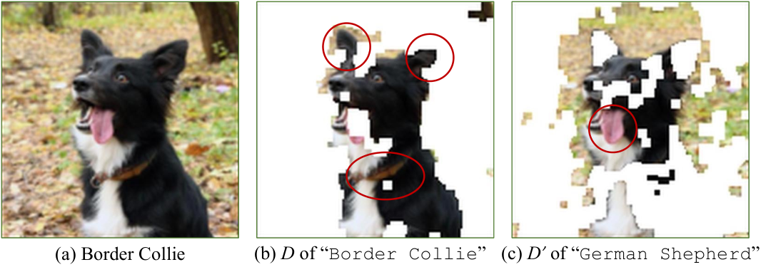
Checking DNN Decisions. $\mathcal{E}_{d}$ is a criterion asserting the equality of $\phi[\![i]\!].D$ and $\phi[\![i^{\prime}]\!].D$ . We introduce an XAI-based approach to constructing $\phi[\![i]\!].D$ , denoting the decision of DNN over $i$ , in Sec. 4. Nevertheless, considering each decision composes a collection of image fragments (each fragment is a visual concept; see Sec. 4), asserting the equality is too strict because image fragments could slightly drift without undermining the DNN overall decisions. The computer vision community primarily uses the Intersection over Union (IoU) metrics to quantify two regions’ overlapping. The calculation of IoU will be given in Sec. 4.2. We deem two decisions violate $\mathcal{E}_{d}$ , in case their overlapping is smaller than a threshold $T_{iou}$ . We empirically decide $T_{iou}$ and present discussions in Sec. 6.2.

Case Study. We observe that several $\langle i,i^{\prime}\rangle$ have zero IoU values for their decisions. Though they lead to the same prediction, this is likely due to chance. Fig. 5 shows a DNN’s inconsistent decisions when its predictions are same. Fig. 5(a) is classified as “thimble” based on the highlighted thimble in Fig. 5(b). However, when the contrast of Fig. 5(a) is slightly lowered, the DNN still predicts “thimble” but relies on a new visual concept, the thumb, as depicted in Fig. 5(c). This inconsistency in DNN decisions, which was not previous detected by prediction consistency-based MT, suggests that the DNN relies incorrectly on the thumb to recognize the thimble. We deem this as a hidden defect of this DNN.

4. Forming and Comparing Decision $D$

We clarify the limitation of merely using pixels to form decisions in Sec. 2.4. Holistically, DNNs are designed to focus on pixel regions (e.g., using convolutional kernels (LeCun et al. 1989b; LeCun et al. 1989a)), and each pixel should exhibit a closely correlated contribution with its neighbors. Importantly, pixel-wise contributions can be abstracted into region-wise visual concepts, reflecting a more holistic, robust, and human-readable view of DNN decisions. We define the decision $D$ as the collection of all visual concepts in a test input $i$ . We have defined visual concepts in Sec. 2.4. We present a technical solution to convert pixels (XAI outputs) to visual concepts in Sec. 4.1, and in Sec. 4.2, we compare two formed decisions $D$ and $D^{\prime}$ .

4.1. Converting Pixels to Visual Concepts

DeepLIFT marks each pixel in an image with a contribution score. In practice, because small positive contributions (e.g., $0.001$ ) are less informative, we denote pixels with contributions substantially higher than a threshold $T_{p}$ as supporting, whereas those with lower or negative contribution scores are deemed non-supporting. That is, we binarize contributions of a pixel based on the contribution score DeepLIFT assigns to each pixel.

4.1.1. Deciding $T_{p}$

The above scheme necessitates the use of a threshold $T_{p}$ to decide the supporting pixels. A naïve approach may be to decide a global threshold. Nevertheless, pixel-wise contributions vary distinctly between inputs, rendering a “global threshold” less applicable. Consider the case in Fig. 3(b), where pixels of the siren may dominate the contributions given a “police car” image. However, siren may contribute less than the cross mark to determine an “ambulance” image. The reason is that while cross mark is exclusive to an ambulance, siren is shared by both classes.

To overcome this hurdle, our implementation adopts Otsu’s method (Otsu 1979) to automatically decide the threshold. In brief, the Otsu’s method seeks the threshold that minimizes intra-class (i.e., supporting or non-supporting) variance while simultaneously maximizing the inter-class (i.e., supporting vs. non-supporting) variance, resulting in a theoretically optimal threshold with moderate cost.

4.1.2. Joining and Detaching Supporting Pixels

Using a threshold $T_{p}$ decided in Sec. 4.1.1, we classify pixels into supporting vs. non-supporting ones. Then, we convert pixels into visual concepts by joining neighboring pixels that positively support the prediction and detaching isolated supporting pixels. We first introduce two elementary image processing operations, erosion and dilation, in this section. For simplicity, we represent the values of supporting and non-supporting pixels using true and false.

Erosion operation mimics soil erosion. As in Fig. 6(b), this operation erodes away the boundaries of positive regions. We implement erosion by using a kernel (similar to a 2D convolution) to slide through the image and retain a positive pixel under a kernel only if all pixels under the kernel is positive (i.e., their conjunction is positive). That is, $\texttt{erosion}(p_{k_{1},k_{2},\dots,k_{m}})\leftarrow\{p_{k_{1}}\land p_{k_{2}}\land,\dots,\land p_{k_{m}}\}^{m}$ .

Dilation is the inverse of erosion. It uses a kernel to slide through the image but sets a pixel under the kernel as positive as long as any pixel under the kernel is positive (i.e., their disjunction is positive): $\texttt{dilation}(p_{k_{1},k_{2},\dots,k_{m}})\leftarrow\{p_{k_{1}}\lor p_{k_{1}}\lor,\dots,\lor p_{k_{m}}\}^{m}$ . As illustrated in Fig. 6(c), dilation enlarges and sharpens positive regions, which further increase their visibility.

Erosion and dilation are two common operations in image processing. They both employ a kernel to slide through an input image, resulting in an output image where the value of each pixel is determined by comparing it to its neighbors in the input image. Then, depending on the order in which these two basic operations are used, we obtain the following two advanced operations.

Closing consists of a dilation with a subsequent erosion. That is, $\texttt{closing}(i)=\texttt{erosion}\circ\texttt{dilation}(i)$ . Consider Fig. 7(a), the closing operation facilitates fill in small holes by joining supporting pixels as regions, yielding an image as in Fig. 7(b).

Opening has an erosion followed by a dilation, i.e., $\texttt{opening}(i)=\texttt{dilation}\circ\texttt{erosion}(i)$ . For example, Fig. 7(c) will be converted into Fig. 7(d) after applying opening. This operation removes small, isolated supporting pixels while retaining the shape and size of large regions formed by supporting pixels. We employ this operation to remove isolated supporting pixels which may be likely induced by estimation errors of XAI.

From Supporting Pixels to Visual Concepts. To convert supporting pixels into visual concepts, we first apply closing and then opening, i.e., $\texttt{to\_concepts}(i)=\texttt{opening}\circ\texttt{closing}(i)$ . The intuition is that, after joining pixels as regions, the remaining isolated pixels can be regarded as useless (or noisy) for identifying DNN decisions. The adopted operations are all standard image processing operations. These operations traverse all pixels in an image in constant time, and can be computed in parallel. $\texttt{to\_concepts}(\cdot)$ can be implemented by replacing the kernel in a 2D convolutional layer, which slides through the image and is multiplied with its covered region, with a sequence of conjunction and disjunction operations detailed in this section. 2D convolutional layers are common in image-processing DNNs. Computation cost incurred at this step is thus equivalent to adding one DNN layer. Moreover, the kernel size in closing and opening decides the effectiveness of extracting visual concepts: a larger kernel is more abstract and thus more robust to potential XAI errors, but less precise. We set the kernel size of closing and opening to $5$ and $3$ , which are two most widely used kernel sizes in convolutional neuron networks that characterize the “spotting region” of common DNNs.

4.2. Measuring Inconsistent $D$ using IoU

Our observation shows that hidden DNN defects unveiled using our MR in Eq. 1 belong to either of the following categories or their composition.

1) Missing visual concepts occurs when the tested DNN relies on a subset of the original visual concepts for prediction. As in Fig. 3, suppose the tested DNN neglects the cross mark under certain perturbations, it has to output “police car” or “ambulance” by chance according to our analysis. By checking “missing visual concepts,” we unveil DNN defects even if the prediction is still “ambulance.”

2) New visual concepts occurs if the tested DNN uses irrelevant visual concepts in the image to make decisions. Recall our motivating example in Fig. 1, where the DNN relies on a flower in Fig. 1(d) as a new visual concept for prediction. Such incorrect decision can also be uncovered by checking the decision consistency.

Overall, the above cases should not happen since we mutate test inputs using semantics-preserving $MR_{t}$ . See $MR_{t}$ adopted in this research in Sec. 5. We use IoU to measure the overlapping of decisions $D$ and $D^{\prime}$ captured in a test input and its mutated input. The calculation of IoU is illustrated in Fig. 8. Overall, each IoU value is a number from 0 to 1 that quantifies the degree of overlapping between two regions.

Clarification on MR. Careful readers may wonder if the above oracle is a bit too strong, because adding/missing a non-important visual concept may not affect DNN predictions from human perspectives, e.g., missing one cross mark may not alter predicting “ambulance” for Fig. 3. Nevertheless, besides classification, features (i.e., the outputs of intermediate layers) extracted from classifiers typically facilitate (security-sensitive) downstream tasks like object tracking and auto-driving, where adding/missing visual concepts can be more serious and likely lead to severe outcomes (He et al. 2017; Girshick 2015; Ren et al. 2015). Moreover, to take into account cases where inconsistent visual concepts are valid, we employ human evaluations to decide a threshold (see RQ2 in Sec. 6.2) to better decide visual concept “inconsistency.”

Table 2. Metamorphic transformations

MR_{t}

adopted.

$MR_{t}$	Original $x$ $\Rightarrow$ Mutated Image $x^{\prime}$	Used by
Pixel Level	$x$ $\Rightarrow$ blur , brightness , contrast	(Pei et al. 2017),(Tian et al. 2018), (Xie et al. 2018),(Demir et al. 2019)
Affine Type	$x$ $\Rightarrow$ rotation , scale , translation , shear	(Pei et al. 2017),(Tian et al. 2018), (Xie et al. 2018),(Demir et al. 2019)
Weather Filter	$x$ $\Rightarrow$ rainy , snowy , foggy , cloudy	(Tian et al. 2018)
Style Transfer	$x$ $\Rightarrow$ style 1 , style 2 , style 3 , style 4	(Zhang et al. 2018)
Adv. Perturb.	$x$ $+=$ PGD , C/W , FGSM , BIM	(Goodfellow et al. 2015),(Madry et al. 2017), (Carlini and Wagner 2017),(Kurakin et al. 2016)

5. Implementation & Setup

The entire codebase of this research, including scripts to form decision-based $MR_{r}$ and extend prior $MR_{t}$ , has about 1500 lines of Python code. We use DeepLIFT, a popular XAI framework, to flag pixel-wise contributions. We reuse and extend $MR_{t}$ implementation of existing MT-based DNN testing frameworks. Most existing MT-based DNN testing works test image classification models by mutating images. $MR_{t}$ in prior works are essentially semantics-preserving image mutations, as reviewed below.

Pixel-Level Mutations. This scheme contains multiple instances. By adding a same constant to all pixels of an image, we can change image brightness. Similarly, multiplying all pixels with a same constant can change image contrast. Blurring is implemented by multiplying the image with a sliding kernel. These three mutations are adopted to assess the robustness of DNNs (Pei et al. 2017; Tian et al. 2018; Xie et al. 2018; Odena and Goodfellow 2018; Demir et al. 2019).

Affine Transformations. This scheme mutates objects in images by applying invertible transformations such as translating, rotating, scaling, and shearing. These transformations preserve the collinearity of objects, thereby retaining correct semantics of objects after mutation. These methods are used to diverse images (Tian et al. 2018; Demir et al. 2019; Xie et al. 2018).

Clarification. Recall that our $MR_{r}$ checks the consistency of decision $D$ . Nevertheless, affine transformations, by mutating objects in an image, unavoidably change the localization of visual concepts. Thus, we calculate the IoU after inverting the applied affine transformation on generated visual concepts. For instance, if the applied affine transformations left rotate 90 degrees, we measure the IoU after first right rotating the visual concepts by 90 degrees.

Weather Filters. To simulate various weather conditions in real scenarios, weather filters, including snowy, foggy, rainy, and cloudy, are widely adopted to mutate test inputs of DNNs. We adopt weather filters proposed in (Tian et al. 2018; Jung et al. 2020) for mutation.

Style Transfer. Style transfer was first proposed by (Zhang et al. 2018), which is specifically launched to transfer (severe) weathers from a source image to a target image. The generated weather conditions in the target are usually in a higher quality than using weather filters. This approach, however, is limited to driving scenes. We extend it to general style-transfer such that arbitrary real images can be mutated. Style transfer primarily mutates image colors and retain the semantics. Our mutations include 72,521 styles; see our code (sna [n.d.]).

Remarks. The weather filters and style transfer are only applied on CIFAR10 and ImageNet which consist of real images. Images in MNIST, a small synthetic dataset, are handwritten digits where no “weather” exists. It is also infeasible to change the color scheme via style transfer, given images in MNIST are black-and-white without the color channel (e.g., the RGB channel in real images).

Adversarial Perturbations. Guided by DNN gradients, adversarial perturbations generate adversarial examples (AEs) to fool DNNs. AEs are usually less notable or visually identical to source images. As shown in Table 2, adversarial perturbations often highlight key objects in an image. We employ four popular algorithms, FGSM (Goodfellow et al. 2015), PGD (Madry et al. 2017), C/W (Carlini and Wagner 2017) and BIM (Kurakin et al. 2016), to generate AEs.

The above mutations are frequently used in previous works: with carefully chosen parameters (i.e., to what extent the mutation is applied), they generally retain the semantics (visual consistency) in the mutated images. Therefore, a functional DNN should preserve its decisions under these mutations. In experiments, we ship $MR_{t}$ configurations from previous works (Pei et al. 2017; Xie et al. 2018; Tian et al. 2018; Demir et al. 2019; Hu et al. 2022) and only mutate a seed (a real image) once; see our implementation in (sna [n.d.]).

Preparing Datasets $\hat{I}_{=}$ and $\hat{I}_{\neq}$ . We prepare an image set $I$ by randomly selecting images from a dataset listed in Table 3. These three datasets are the most widely-used datasets for DNN testing. For each $i\in I$ , we mutate it with different $\texttt{t}\in MR_{t}$ , as presented in Table 2, and produce $i_{\texttt{t}}=\{\texttt{t}(i)|\texttt{t}\in MR_{t}\}$ .⁴⁴ 4 Note that a $MR_{t}$ t may be used for multiple times, each with a randomly selected configuration, e.g., rotation degree or brightness level. Then, for each $i$ and its mutated $i^{\prime}\in i_{\texttt{t}}$ , we construct a set $\hat{I}$ with image pairs $\langle i,i^{\prime}\rangle$ , namely, $\hat{I}=\{\langle i,i^{\prime}\rangle|i\in I,i^{\prime}\in i_{\texttt{t}}\}$ . We further divide $\hat{I}$ into two collections: 1) $\hat{I}_{=}$ where the DNN $\phi$ has the same prediction label for $i$ and $i^{\prime}$ , i.e., $\hat{I}_{=}=\{\langle i,i^{\prime}\rangle|\phi[\![i]\!].L=\phi[\![i^{\prime}]\!].L,\langle i,i^{\prime}\rangle\in\hat{I}\}$ , and 2) $\hat{I}_{\neq}$ where the DNN $\phi$ yields inconsistent labels for $i$ and $i^{\prime}$ , i.e., $\hat{I}_{\neq}=\{\langle i,i^{\prime}\rangle|\phi[\![i]\!].L\neq\phi[\![i^{\prime}]\!].L,\langle i,i^{\prime}\rangle\in\hat{I}\}$ . For each tested DNN, we keep generating $\hat{i}$ until both $\hat{I}_{=}$ and $\hat{I}_{\neq}$ has $10,000$ pairs.

Preparing Tested DNNs. We list all DNN models tested in this paper in Table 3. Note that for the first three models, we use two instances trained over two different datasets, ImageNet and CIFAR10. All ImageNet-trained models are officially provided by PyTorch and other models are well-trained (over 94% test accuracy). They are commonly used in daily DNN tasks and testings.

Table 3. Evaluated DNN models.

Model	Dataset	Remark
ResNet50 (He et al. 2016)	ImageNet (Deng et al. 2009)/CIFAR10 (Krizhevsky et al. 2009)	Non-sequential structure
VGG16 (Simonyan and Zisserman 2014)	ImageNet/CIFAR10	Sequential structure
MobileNet-V2 (Howard et al. 2017)	ImageNet/CIFAR10	Mobile devices
DenseNet121 (Huang et al. 2017)	ImageNet	Extremely deep model
Inception-V3 (Szegedy et al. 2016)	ImageNet	Feature representation
LeNet1 (LeCun et al. 1989b)	MNIST (Deng 2012)	Black-white images
LeNet5 (LeCun et al. 1998)	MNIST	Black-white images

6. Evaluation

We primarily study the following research questions.

RQ1: Is the identified decision $D$ in each DNN input correct? We answer this question in Sec. 6.1.

RQ2: Are inconsistency of decisions $D_{1}\neq D_{2}$ truly reflect DNN defects? We launch large-scale human evaluation to explore this question from different aspects in Sec. 6.2.

RQ3: How many and how frequent hidden defects are overlooked by existing MT-based DNN testing? What are the characteristics of these hidden defects? We answer this question in Sec. 6.3.

Table 4. Correctness of identified decisions. We report the percentage of unchanged outputs (left) when only keeping the decisions, and the percentage of changed outputs (right) when masking decisions in inputs.

ResNet50 ImageNet	VGG16 ImageNet	MobileNetV2 ImageNet	DenseNet121 ImageNet	Inception-V3 ImageNet
96.0%, 100%	96.8%, 100%	96.5%, 100%	96.9%, 100%	95.8%, 100%
ResNet50 CIFAR10	VGG16 CIFAR10	MobileNetV2 CIFAR10	LeNet1 MNIST	LeNet5 MNIST
97.6%, 93.8%	95.8%, 92.6%,	96.8%, 92.7%	96.2%, 91.8%	96.9%, 93.5%

6.1. RQ1: Correctness of Decisions

It is challenging to assess the correctness of obtained decisions: as clarified in Sec. 2.2, we lack the ground truth decisions $D_{G}$ for diverse real-world images. Furthermore, given that DNNs are designed to discover (subtle) patterns inherent in the data, it is likely that they make decisions using visual concepts that are diametrically different from human judgments, but still valid.

To measure the correctness of captured decisions, we aim to construct contradictory facts to the DNN to assess the accuracy of decisions. Our intuition is that if and only if the identified visual concepts correctly constitute the decisions of the DNN, the DNN prediction should not be changed when only these visual concepts are extracted to form DNN inputs. Accordingly, if the identified visual concepts in an input are masked, the DNN prediction should change (as it loses the decisions).

For each tested DNN, the above schemes are performed for the original inputs and the mutated input pairs from both $\hat{I}_{=}$ and $\hat{I}_{\neq}$ . Results are reported in Table 4. We also use the above masking schemes directly toward pixels identified by conventional XAI techniques, including raw outputs of DeepLIFT. For both two masking schemes, they only have around 50% of outputs unchanged/changed. In contrast, the converted visual concepts are more reliable, as it better correlates with our expectation: when identified visual concepts are masked, over $1-\frac{1}{C}$ of outputs are changed (100% in ImageNet cases), where $C$ is the #classes. Since the DNN has $\frac{1}{C}$ chance to guess the output, our identified decisions are precise. Similarly, when inputs only contain the identified decisions, all models have over $95\%$ outputs unchanged. Most identified visual concepts are small fragments in images (they may be “invalid” as an input image). Thus, it is reasonable that the results are slightly lower than 100%. Overall, we interpret that decisions extracted by our technique represent the true decisions of various DNNs.

6.2. RQ2: Human Evaluation

We now analyze how IoU values, which are derived by comparing the visual concepts of an image pair $\langle i,i^{\prime}\rangle$ , of $\hat{I}_{=}$ and $\hat{I}_{\neq}$ , are distributed. We first report that for all image pairs in $\hat{I}_{\neq}$ , the maximal IoU value $v<0.8$ , indicating that visual concepts among $i$ and $i^{\prime}$ are always different whenever the DNN yields different labels. Moreover, we report that the IoU value $v$ calculated over images in $\hat{I}_{=}$ ranges from $0$ to $1$ . Obviously, an IoU value $v=1$ indicates that the decisions of $i$ and $i^{\prime}$ are exactly the same, falling into the ① case in Table 1 where $L_{1}=L_{2}$ and $D_{1}=D_{2}$ . An IoU $v=0$ , in contrast, illustrates that the decisions in $i$ and $i^{\prime}$ are deemed as different. For such cases, it is clear that the DNN makes an incorrect prediction, falling into scenario ③ of Table 1 where $L_{1}=L_{2}$ and $D_{1}\neq D_{2}$ .

When the IoU value $0<v<1$ , it is unclear if DNN makes incorrect predictions. A simple method is to consider two decisions distinct as long as $v<1$ . However, our manual analysis shows that for $\hat{I}_{=}$ , $v<1$ does not necessarily imply that the DNN makes different decisions over $i$ and $i^{\prime}$ . For instance, the non-overlapping may be caused by different fragments on grass and clouds and other large objects in $i$ . Despite the existence of non-overlapping visual concepts, they all represent the same object. Similarly, a relatively higher (near to $1$ ) IoU value does not always indicate no defect, as some small yet critical visual concepts may cover only a small portion of areas among all identified ones (e.g., the cross mark in an ambulance; see Fig. 3).

We conduct human evaluations to explore to what extent the IoU value can reflect the inconsistency of two decisions $D$ and $D^{\prime}$ . We form a group of $25$ participants to answer a total of $10,000$ questions. Given images from CIFAR10 and MNIST have relatively lower resolution, we only use images from ImageNet — the de facto real-life dataset which has the largest scale among all evaluated datasets. All evaluations are performed on the Amazon Mechanical Turk platform. We explain the setup and give quantitative results in Sec. 6.2.1. We present qualitative feedback in Sec. 6.2.4.

6.2.1. Are Decisions Same?

Since understanding the visual concept and DNN decisions may be obscure for laymen, we invite $15$ Ph.D. students with experience in computer vision and DNN related projects to participate this evaluation. Prior to the experiment, we teach a student what a visual concept is through examples and explain how to distinguish consistent/inconsistent DNN decisions, until the student is confident that he/she understands the prior knowledge. The teaching takes in average $30$ minutes for each participant; we provide full materials used at this step to benefit future research on our released artifact (sna [n.d.]).

We use five popular and representative DNNs trained on ImageNet, as listed in Table 3. For each model, we randomly select $500$ pairs of images, which are evenly generated by each type of $MR_{t}$ we introduced in Sec. 5, from $\hat{I}_{=}$ and collect a set of total $2,500$ pairs. We then repeat each pair three times so that three participants can analyze each pair of decisions. The totaling 7,500 images are evenly assigned to $15$ participants. Each participant may halt the human evaluation anytime to avoid fatigue. On average, each participant requires $2.5$ hours to finish the entire evaluation.

For each question, we present the student three images: the original image $i$ and two images displaying only the decisions of $i$ and $\hat{i}$ . Then, we ask whether the two decisions are equivalent (i.e., they rely on the same set of visual concepts). Students may select “Yes”, “No”, or “Not sure”, which count 1, -1, 0, respectively. As aforementioned, since DNNs are designed to explore (subtle) patterns in data, it can be difficult for humans to deduce the image content given only the visual concepts captured by DNNs. By providing the original image $i$ , students grasp the “whole picture” in the image, and we find this helps them compare decisions in $i$ and $\hat{i}$ . Otherwise, they may just compare the pixel-wise difference, if they have no idea about what is displayed in the image.

Moreover, we find that students may fail to truly understand the requirements of this experiment, resulting in potentially invalid findings. As a common practice, we prepare and insert a number of sanity-check (SC) questions randomly into the raised questions without prior notice. Students must correctly answer SCs in order to justify the reliability of their answers. Specifically, in some questions, we present two identical decisions (i.e., extracted from the same image), for which participants should answer “yes.” We also reorder the two images of decisions in some questions to generate duplicated questions — reordering makes students less likely to notice that they have already answered this question; for duplicated questions, student should answer consistently with the original questions. We discard answers from students who correctly answer $<95\%$ SC questions. All participants have passed the sanity check.

To analyze the results, we group questions by 1) model and 2) the type of $MR_{t}$ . We show how the scores of questions change with IoU values in Fig. 9. It is evident that each question’s score has a strong positive correlation with the IoU value. When the decisions of $\langle i,i^{\prime}\rangle$ have a small IoU value ( $<0.2$ ), nearly all participants agree that they denote different decisions. Similarly, most participants regard two decisions as the same if they have a sufficiently higher IoU value ( $>0.8$ ). From Fig. 9, we notice that in all cases (i.e., grouped by $5$ models, or $5$ types of $MR_{t}$ ), scores of $\langle i,i^{\prime}\rangle$ pairs are less than 0 when the corresponding IoU values are smaller than $0.5$ . Moreover, the score is around $-0.75$ , when the IoU values are smaller than $0.2$ . This indicates the majority of participants agree that the two decisions are different. As a practical setup, we recommend IoU values in the vicinity of $0.2$ .

6.2.2. How Apparent the Decisions Change?

To better justify our findings, we further conduct an experiment to evaluate how apparent the decision changes are via assessing whether they are human-perceptible at the first glance. The intuition is that, if the difference can be noticed at the first glance, it is likely induced by distinct visual concepts and thus indicates a DNN defect. This experiment follows mostly the same setup as in Sec. 6.2.1 but only shows the decisions of $i$ and $i^{\prime}$ two seconds. Moreover, to make the results more general (students with different backgrounds may have distinct preference; see Sec. 6.2.4), we invite another 10 Ph.D. and masters students with various backgrounds to evaluate total $2,500$ pairs of decisions from $\hat{I}_{=}$ ; see detailed setups in (sna [n.d.]). We present results in Fig. 10. Compared to Fig. 9, results in Fig. 10 has a slightly higher fluctuation, which may be due to the participants’ small time window (2 seconds). Nevertheless, we observe that trends in Fig. 9 and Fig. 10 are highly consistent, indicating that the decisions are highly recognizable and of high quality.

6.2.3. Agreements of Participants

We use Fleiss’ kappa to evaluate the reliability of our human evaluation results. The Fleiss’ kappa is widely used to assess the agreement among choices of multiple ( $>2$ ) participants. A kappa value of $1$ indicates that all participants totally agree on a choice, whereas kappa values $\leq 0$ imply participants made completely random choices.

The overall Fleiss’ kappa coefficients for the human evaluations in Sec. 6.2.1 and Sec. 6.2.2 are $0.756$ and $0.762$ , indicating a substantial agreement among all participants on all $\langle i,i^{\prime}\rangle$ pairs (Gwet 2014; Sim and Wright 2005). We further present how the kappa coefficients for various DNNs and $MR_{t}$ types vary with the IoU value of decisions $D$ and $D^{\prime}$ in Fig. 11 and Fig. 12. We note that the results are consistent regardless of the DNN or $MR_{t}$ : when the IoU values of $\langle i,i^{\prime}\rangle$ ’s decisions lie in $[0,0.2]\cup[0.8,1.0]$ , the kappa coefficients of all participants are close to $1$ (and in some cases reach $1$ ); this indicates a nearly perfect agreement (Gwet 2014). Overall, all participants concur that two decisions are different if their corresponding IoU score is less than $0.2$ . In sum, we view the Fleiss’ kappa scores are aligned with our observation in Sec. 6.2.1: IoU score threshold 0.2 is generally accurate to highlight distinct decisions.

6.2.4. Feedbacks from Participants

We present some representative feedbacks from participants; they are asked to describe what they primarily rely on to compare decisions. Considering the following response from a student working on software testing:

“I first exclude image pairs that are obviously different, e.g., one color, which should cover a large area, only appear in one of the masked image. Then I compare whether the different regions correspond to any complete feature, for instance, a whole eye rather than part of an eye. I regard two masked images as the same one if their difference is only induced by parts of several features.”

Notice that he uses a “process of elimination” (“[…] first exclude […]”) to help make comparison. Recall that we give an example of how a DNN relies on visual concepts to make decisions (“ambulance”) under Fig. 3. This feedback indicates, to some extent, that the visual concepts derived by our method are logically reasonable and adequately explain the DNN decisions. Moreover, considering a response from a student working on computer vision:

“I pay more attention to special textures, for example, marks on plumage of a bird, because I know for most DNNs, they are critical for making the prediction. ”

We clarify that these two students’ comparison results are mostly consistent. Nevertheless, their strategies and focuses are distinct; the second participant is attentive to properties like texture. This reflects the overall difficulty of our research problem, as different experts may base their comparison on distinct features. It also indicates the high quality of our extracted decisions, as they are often interpretable by human from multiple perspectives.

(a) ResNet & ImageNet.

(b) VGG & ImageNet.

(d) DenseNet & ImageNet.

(e) Inception & ImageNet.

(f) ResNet & CIFAR10.

(g) VGG & CIFAR10.

(h) MobileNet & CIFAR10.

(i) LeNet1 & MNIST.

(j) LeNet5 & MNIST.

Figure 13. Histograms of IoU values (grouped by DNN) over

D

\langle i,i^{\prime}\rangle\in\hat{I}_{=}

. Red line denotes cumulative distribution (CDF).

(a) Pixel-Level.

(b) Affine

(d) Style Transfer.

(e) Adv. Perturbation.

Figure 14. Histograms of IoU values (grouped by

MR_{t}

) over

D

\langle i,i^{\prime}\rangle\in\hat{I}_{=}

. Red line denotes cumulative distribution (CDF).

6.3. Analysis of Hidden Defects

This section revisits existing MT-based testing frameworks through the lens of our decision-based $MR_{r}$ . Fig. 13 and Fig. 14 show how IoU values, which are grouped by models or the types of $MR_{t}$ over $\langle i,i^{\prime}\rangle\in\hat{I}_{=}$ , are distributed.

6.3.1. Results Overview

We note that for each model, or each type of $MR_{t}$ , almost half of the $\langle i,i^{\prime}\rangle$ pairs have IoU values less than $0.5$ . Given that DNNs are still making “consistent” predictions over $i$ and $i^{\prime}$ , we thus deem that a large number of hidden defects are not detected by existing MT frameworks merely checking DNN prediction consistency. We now analyze hidden defects’ characteristics.

Comparing Different DNNs. Fig. 13 illustrates that the distributions of IoU values primarily vary in accordance with the DNN architectures (e.g., ResNet50 vs. VGG16) rather than with the training datasets (e.g., CIFAR10 vs. ImageNet). For instance, Fig. 13(a), Fig. 13(b), and Fig. 13(c) have more distinct trends, whereas Fig. 13(b) and Fig. 13(g) have correlated trends. This is an interesting observation: our evaluated DNNs are all commonly used in real-world scenarios, and they have different representative structures. Thus, it is reasonable to assume that, hidden defects due to inconsistent decisions are mostly induced by different model design. Accordingly, to fix these defects, developers are expected to focus on DNN architectures rather than simply enriching the datasets (ImageNet is much more comprehensive than CIFAR10). We present further discussions on DNN defect repairing in Sec. 7.

Comparing Different $MR_{t}$ . Fig. 14 shows that IoU values corresponds to different $MR_{t}$ have distinct distributions.

Adversarial Perturbations: Fig. 14(e) shows that the majority of IoU values are close to two extremes, $0$ and $1$ . That is, the decisions of $\langle i,i^{\prime}\rangle$ , when their corresponding outputs are identical, are either exactly same or completely different in many cases. It also has the highest ratio of zero IoU value, indicating its high effectiveness of flipping DNN predictions. Note that adversarial perturbations are guided by DNN gradients, which are very informative for describing DNN behaviors. This can also be reflected from Table 2 where key objects in image are highlighted by adversarial perturbations. In addition, compared with other $MR_{t}$ discussed below, adversarial perturbation may be more desirable, since it does not introduce much false positive/negative cases due to challenges in deciding a proper IoU threshold — as reflected from our empirical results, users may safely regard two decisions of $\langle i,i^{\prime}\rangle$ as inconsistent as long as their IoU value is zero. This saves the extra effort of human assessments and confirmation.

Affine Transformations: As in Fig. 14(b), this $MR_{t}$ has the highest ratio of IoU values less than $0.2$ , where the decisions of $\langle i,i^{\prime}\rangle$ differ based on our human evaluation. It also has the second-highest ratio of zero IoU values. Recall we invert an affine transformation on decisions of $i^{\prime}$ before computing IoU. Therefore, we may infer that modern DNNs are still highly sensitive to affine transformations, which can change the position, viewing angle, size, orientation of objects, thereby introducing more diverse “patterns” in images. Compared with other $MR_{t}$ (e.g., style transfer and adversarial perturbation), affine transformations manifest a relative lower cost and are applicable in most scenarios. It may be reasonable to conclude that affine transformation is a suitable pre-processing approach for generating large-scale, diverse images to better stress DNNs. Such a diverse image collection could be of high benefit in augmenting DNN training data and repairing DNNs. In fact, this strategy has been adopted by many existing works (Shorten and Khoshgoftaar 2019).

Style Transfer: As in Fig. 14(d), the highest IoU of this $MR_{t}$ approaches $0.8$ . That is, when $i$ is mutated into $i^{\prime}$ using style transfer, their corresponding decisions are always distinct (in all our evaluated cases). Recent works have pointed out that DNNs trained on real datasets (e.g., ImageNet) have a texture bias: they primarily rely on texture rather than the shape of objects to make predictions. Accordingly, previous works proposed training DNNs on style-transferred images to alleviate texture-bias (Geirhos et al. 2018). As shown in Table 2, style transfer changes the color schemes of an image (e.g., from realistic to artistic), which modifies the texture while retaining the object shape. Our findings illustrate the strength of style transfer, which, to a great extent, validates the motivation and argumentation of previous research. Interestingly, as demonstrated in our evaluation in Sec. 6.2, the highest IoU value calculated over decisions of $\langle i,i^{\prime}\rangle\in\hat{I}_{\neq}$ is also close to $0.8$ . Taking Fig. 14(d) into account, we hypothesize that an IoU less than $0.8$ indicates different decisions from the DNN perspective (though are less human-notable). From our empirical observation, we suggest that safety-critical DNNs (e.g., autonomous driving) employ an IoU of $0.8$ .

Pixel-wise Mutation & Weather Filter: Fig. 14(a) and Fig. 14(c) have similar IoU value distributions: the majority of IoU values cluster around $0.5$ and values in $[0,1]$ are all covered. Both two $MR_{t}$ can be viewed as adding diverse “noise” on images. Despite being less effective than other $MR_{t}$ at triggering inconsistent decisions, they still expose a number of DNN defects. Moreover, it is evident that error-triggering inputs generated by pixel-wise mutations or weather filters are distinct with those of style transfer and affine transformations, as they impose different mutation effects on images. Therefore, all $MR_{t}$ proposed by prior works are demanding to stress DNNs from different angles. Also, since pixel-wise mutation and weather filter have lower cost, similar to affine transformation, it is feasible to generate large-scale, diverse image collections using these two methods. We thus believe that they are useful for augmenting DNN training data and repairing DNNs.

6.3.2. Case Study

As revealed in Fig. 13, taking decision consistency into account enables detecting a large number of DNN defects from all popular DNNs. Fig. 1, Fig. 3, and Fig. 5 have shown several cases, where the decisions in the original images are largely inconsistent with the mutated images, though DNNs still (incorrectly) yields consistent labels. Due to limited space, we provide more cases at (sna [n.d.]): the inconsistent decisions are mostly induced by both cases that miss and add visual concepts, as described in Sec. 4.2, and they occur in images of different classes that are mutated using various methods. Overall, the diversity indicates that our decision-based oracle can find a broad set of defects. We will maintain our unveiled cases to benefit follow-up research and comparison.

Table 5. The number of DNN inferences within one minute on one Nvidia GeForce RTX 2080 GPU.

	ResNet50 ImageNet	ResNet50 CIFAR10	LeNet5 MNIST
Inference w/o decision	$\sim 6,000$ /min	$\sim 8,000$ /min	$\sim 30,000$ /min
Inference w/ decision	$\sim 1,600$ /min	$\sim 2,000$ /min	$\sim 13,000$ /min

•

*ResNet50 is the largest DNN for ImageNet/CIFAR10 in our evaluation.
•

*LeNet5 is larger than LeNet1.

7. Discussion and Future Work

Cost vs. Benefit. The extra cost of our decision-based oracle consists of one backward propagation of DeepLIFT, and the conversion from prediction-contributing pixels to visual concepts. As clarified in Sec. 4.1, cost of is comparable to executing one extra DNN layer. Given that modern DNNs have tens of layers (e.g., ResNet50 has 50 layers), introduces the majority of extra cost. We compare DNN inference speed with and without extracting decisions in Table 5: extracting decisions slows DNN inference by a factor of four. Since has a relatively high tolerance for errors in XAI outputs (recall we abstract XAI outputs into visual concepts), the overhead can be further reduced by using various quicker (but possibly less accurate) XAI methods available off-the-shelf.

From the “benefit” perspective, we note that in Sec. 6’s experiments, only about $1.5\%$ mutated inputs result in incorrect predictions. $20\sim 30\%$ of the remaining $98.5\%$ inputs (which induce consistent predictions) have IoU values smaller than $0.2$ (i.e., their decisions are inconsistent), according to the cumulative distribution function (the red line) in Fig. 13 and Fig. 14. Thus, taking decision-based oracle into account would reveal many more defects than before. In sum, given the reasonable cost and the benefit, we believe it is worthwhile to integrate our new oracle into DNN testing.

Extension to Other Tasks. In this research, we primarily consider images and extract visual concepts from images to form $MR_{r}$ . We clarify that our work roots the same focus as most works in this field, which test DNNs for image classification. Nevertheless, from a holistic view, our oracle asserts if DNN keeps the correct “focus” on the seed inputs and the mutated inputs; our oracle is violated if the focus is changed notably, regardless of the DNN tasks being evaluated. Thus, our oracle should be applicable to other tasks, such as activity/emotion recognition where the activity/emotion is recognized based on visual concepts.

For common image classification-based tasks, our XAI-based approach can precisely scope DNN decisions. In complex computer vision scenarios like auto-driving, classification, localization, and tracking tasks are all involved. We leave it as one future work to extend our technical pipeline to handle localization/tracking tasks. For other tasks where DNNs accept discrete inputs (e.g., text, tabular data, or grid), the minimal semantics-meaningful unit on these inputs is one discrete unit (similar to an image pixel), such as a word in a sentence, a cell in a table, or a dot in the grid. Testing such DNNs can be easier, as we may directly form a decision-based oracle using XAI outputs, including several critical discrete units.

Threat to Validity. This research regards the decisions of a DNN prediction as a collection of visual concepts, and evaluate the correctness of decisions by removing/keeping all visual concepts together. One threat is that some identified visual concepts are incorrect. In practice, it is challenging to assess the correctness of each visual concept individually, because removing/keeping part of the identified visual concepts may break the integrity of the decisions and lead to a different decision process.

However, we clarify that a few incorrect visual concepts, if they exist at all, should not affect our decision-based oracle for two reasons. First, DeepLIFT is a well-established XAI tool whose errors are pixel-wise, typically in the form of several inaccurately estimated contribution scores. However, instead of using the exact scores, we simply recognize pixels with positive scores. Moreover, the procedure of abstracting pixel-level contributions to visual concepts can also reduce inaccuracy. Second, we do not regard two decisions as inconsistent based solely on deviations in visual concepts. Instead, we deem decisions are “inconsistent” when their overlapping is below a small threshold. Overall, the threat of potentially incorrect XAI outputs is mostly eliminated in our implementation.

8. Conclusion

To reveal hidden DNN defects due to ill-decisions, this paper proposes to extend MT-based DNN testing by checking DNN decision consistency. Our evaluation shows that decision-based MT exhibits promising detectability for DNN defects. Our findings can provide insights for researchers that aim to launch MT toward DNNs.

Acknowledgements.

We thank the anonymous ASE reviewers and our shepherd for their valuable feedback and constructive comments. We also thank all participants of our human evaluation.

References

(1)
sna ([n.d.]) [n.d.]. Research Artifact. https://github.com/Yuanyuan-Yuan/Decision-Oracle.
Ancona et al. (2019) Marco Ancona, Cengiz Oztireli, and Markus Gross. 2019. Explaining deep neural networks with a polynomial time for shapley value approximation (PMLR).
Bach et al. (2015) Sebastian Bach, Alexander Binder, Grégoire Montavon, Frederick Klauschen, Klaus-Robert Müller, and Wojciech Samek. 2015. On pixel-wise explanations for non-linear classifier decisions by layer-wise relevance propagation. PloS one 10, 7 (2015), e0130140.
Carlini and Wagner (2017) Nicholas Carlini and David Wagner. 2017. Towards evaluating the robustness of neural networks (IEEE SP).
Carter et al. (2019) Shan Carter, Zan Armstrong, Ludwig Schubert, Ian Johnson, and Chris Olah. 2019. Exploring neural networks with activation atlases. Distill 1 (2019), 2.
Chattopadhay et al. (2018) Aditya Chattopadhay, Anirban Sarkar, Prantik Howlader, and Vineeth N Balasubramanian. 2018. Grad-cam++: Generalized gradient-based visual explanations for deep convolutional networks (WACV).
Chen et al. (1998) Tsong Y Chen, Shing C Cheung, and Shiu Ming Yiu. 1998. Metamorphic testing: a new approach for generating next test cases. Technical Report. Technical Report HKUST-CS98-01, Department of Computer Science, Hong Kong ….
Covert and Lee (2021) Ian Covert and Su-In Lee. 2021. Improving KernelSHAP: Practical Shapley value estimation using linear regression (ICAIS).
Datta et al. (2016) Anupam Datta, Shayak Sen, and Yair Zick. 2016. Algorithmic transparency via quantitative input influence: Theory and experiments with learning systems. In IEEE SP.
Demir et al. (2019) Samet Demir, Hasan Ferit Eniser, and Alper Sen. 2019. DeepSmartFuzzer: Reward Guided Test Generation For Deep Learning. arXiv preprint arXiv:1911.10621 (2019).
Deng et al. (2009) J. Deng, W. Dong, R. Socher, L.-J. Li, K. Li, and L. Fei-Fei. 2009. ImageNet: A Large-Scale Hierarchical Image Database. In CVPR09.
Deng (2012) Li Deng. 2012. The mnist database of handwritten digit images for machine learning research [best of the web]. IEEE Signal Processing Magazine (2012).
Dwarakanath et al. (2019) Anurag Dwarakanath, Manish Ahuja, Sanjay Podder, Silja Vinu, Arijit Naskar, and MV Koushik. 2019. Metamorphic testing of a deep learning based forecaster. In MET.
Dwarakanath et al. (2018) Anurag Dwarakanath, Manish Ahuja, Samarth Sikand, Raghotham M. Rao, R. P. Jagadeesh Chandra Bose, Neville Dubash, and Sanjay Podder. 2018. Identifying Implementation Bugs in Machine Learning Based Image Classifiers Using Metamorphic Testing. In ISSTA.
Geirhos et al. (2018) Robert Geirhos, Patricia Rubisch, Claudio Michaelis, Matthias Bethge, Felix A Wichmann, and Wieland Brendel. 2018. ImageNet-trained CNNs are biased towards texture; increasing shape bias improves accuracy and robustness. arXiv preprint arXiv:1811.12231 (2018).
Girshick (2015) Ross Girshick. 2015. Fast r-cnn. In Proceedings of the IEEE international conference on computer vision. 1440–1448.
Goodfellow et al. (2015) Ian J Goodfellow, Jonathon Shlens, and Christian Szegedy. 2015. Explaining and harnessing adversarial examples. In ICLR.
Gunning et al. (2019) David Gunning, Mark Stefik, Jaesik Choi, Timothy Miller, Simone Stumpf, and Guang-Zhong Yang. 2019. XAI—Explainable artificial intelligence. Science Robotics 4, 37 (2019), eaay7120.
Gwet (2014) Kilem L Gwet. 2014. Handbook of inter-rater reliability: The definitive guide to measuring the extent of agreement among raters. Advanced Analytics, LLC.
He et al. (2017) Kaiming He, Georgia Gkioxari, Piotr Dollár, and Ross Girshick. 2017. Mask R-CNN. In CVPR. 2961–2969.
He et al. (2016) Kaiming He, Xiangyu Zhang, Shaoqing Ren, and Jian Sun. 2016. Deep residual learning for image recognition. In CVPR. 770–778.
Hein et al. (2019) Matthias Hein, Maksym Andriushchenko, and Julian Bitterwolf. 2019. Why relu networks yield high-confidence predictions far away from the training data and how to mitigate the problem. In CVPR.
Howard et al. (2017) Andrew G Howard, Menglong Zhu, Bo Chen, Dmitry Kalenichenko, Weijun Wang, Tobias Weyand, Marco Andreetto, and Hartwig Adam. 2017. Mobilenets: Efficient convolutional neural networks for mobile vision applications. arXiv preprint arXiv:1704.04861 (2017).
Hu et al. (2022) Boyue Caroline Hu, Lina Marsso, Krzysztof Czarnecki, Rick Salay, Huakun Shen, and Marsha Chechik. 2022. If a Human Can See It, So Should Your System: Reliability Requirements for Machine Vision Components. arXiv preprint arXiv:2202.03930 (2022).
Huang et al. (2017) Gao Huang, Zhuang Liu, Laurens Van Der Maaten, and Kilian Q Weinberger. 2017. Densely connected convolutional networks. In CVPR.
Jung et al. (2020) Alexander B. Jung, Kentaro Wada, Jon Crall, Satoshi Tanaka, Jake Graving, Christoph Reinders, Sarthak Yadav, Joy Banerjee, Gábor Vecsei, Adam Kraft, Zheng Rui, Jirka Borovec, Christian Vallentin, Semen Zhydenko, Kilian Pfeiffer, Ben Cook, Ismael Fernández, François-Michel De Rainville, Chi-Hung Weng, Abner Ayala-Acevedo, Raphael Meudec, Matias Laporte, et al. 2020. imgaug. https://github.com/aleju/imgaug. Online; accessed 01-Feb-2020.
Krizhevsky et al. (2009) Alex Krizhevsky, Geoffrey Hinton, et al. 2009. Learning multiple layers of features from tiny images. (2009).
Kundel and Nodine (1983) HL Kundel and CF Nodine. 1983. A visual concept shapes image perception. Radiology 146, 2 (1983), 363–368.
Kurakin et al. (2016) Alexey Kurakin, Ian Goodfellow, and Samy Bengio. 2016. Adversarial examples in the physical world. arXiv preprint arXiv:1607.02533 (2016).
LeCun et al. (1989a) Yann LeCun, Bernhard Boser, John Denker, Donnie Henderson, Richard Howard, Wayne Hubbard, and Lawrence Jackel. 1989a. Handwritten digit recognition with a back-propagation network. NIPS (1989).
LeCun et al. (1989b) Yann LeCun, Bernhard Boser, John S Denker, Donnie Henderson, Richard E Howard, Wayne Hubbard, and Lawrence D Jackel. 1989b. Backpropagation applied to handwritten zip code recognition. Neural computation 1, 4 (1989), 541–551.
LeCun et al. (1998) Yann LeCun, Léon Bottou, Yoshua Bengio, and Patrick Haffner. 1998. Gradient-based learning applied to document recognition. Proc. IEEE 86, 11 (1998), 2278–2324.
Li et al. (2022) Zongjie Li, Chaozheng Wang, Zhibo Liu, Haoxuan Wang, Shuai Wang, and Cuiyun Gao. 2022. CCTEST: Testing and Repairing Code Completion Systems. arXiv preprint arXiv:2208.08289 (2022).
Linardatos et al. (2020) Pantelis Linardatos, Vasilis Papastefanopoulos, and Sotiris Kotsiantis. 2020. Explainable ai: A review of machine learning interpretability methods. Entropy 23, 1 (2020), 18.
Lundberg and Lee (2017) Scott M Lundberg and Su-In Lee. 2017. A unified approach to interpreting model predictions. Advances in neural information processing systems 30 (2017).
Ma et al. (2018) Lei Ma, Fuyuan Zhang, Jiyuan Sun, Minhui Xue, Bo Li, Felix Juefei-Xu, Chao Xie, Li Li, Yang Liu, Jianjun Zhao, et al. 2018. Deepmutation: Mutation testing of deep learning systems. In ISSRE.
Ma and Wang (2021) Pingchuan Ma and Shuai Wang. 2021. MT-teql: evaluating and augmenting neural NLIDB on real-world linguistic and schema variations. (2021).
Ma et al. (2020) Pingchuan Ma, Shuai Wang, and Jin Liu. 2020. Metamorphic Testing and Certified Mitigation of Fairness Violations in NLP Models. In IJCAI. 458–465.
Madry et al. (2017) Aleksander Madry, Aleksandar Makelov, Ludwig Schmidt, Dimitris Tsipras, and Adrian Vladu. 2017. Towards deep learning models resistant to adversarial attacks. arXiv preprint arXiv:1706.06083 (2017).
Mao et al. (2015) Junhua Mao, Xu Wei, Yi Yang, Jiang Wang, Zhiheng Huang, and Alan L Yuille. 2015. Learning like a child: Fast novel visual concept learning from sentence descriptions of images. In ICCV.
Montavon et al. (2019) Grégoire Montavon, Alexander Binder, Sebastian Lapuschkin, Wojciech Samek, and Klaus-Robert Müller. 2019. Layer-wise relevance propagation: an overview. Explainable AI: interpreting, explaining and visualizing deep learning (2019).
Nakajima and Chen (2019) Shin Nakajima and Tsong Yueh Chen. 2019. Generating biased dataset for metamorphic testing of machine learning programs. In IFIP-ICTSS.
Nguyen et al. (2015) Anh Nguyen, Jason Yosinski, and Jeff Clune. 2015. Deep neural networks are easily fooled: High confidence predictions for unrecognizable images. In Proceedings of the IEEE conference on computer vision and pattern recognition. 427–436.
Odena and Goodfellow (2018) Augustus Odena and Ian Goodfellow. 2018. Tensorfuzz: Debugging neural networks with coverage-guided fuzzing. arXiv preprint arXiv:1807.10875 (2018).
Otsu (1979) Nobuyuki Otsu. 1979. A threshold selection method from gray-level histograms. IEEE transactions on systems, man, and cybernetics 9, 1 (1979), 62–66.
Pei et al. (2017) Kexin Pei, Yinzhi Cao, Junfeng Yang, and Suman Jana. 2017. DeepXplore: Automated Whitebox Testing of Deep Learning Systems (SOSP ’17).
Ren et al. (2015) Shaoqing Ren, Kaiming He, Ross Girshick, and Jian Sun. 2015. Faster r-cnn: Towards real-time object detection with region proposal networks. In Advances in neural information processing systems. 91–99.
Ribeiro et al. (2016) Marco Tulio Ribeiro, Sameer Singh, and Carlos Guestrin. 2016. " Why should i trust you?" Explaining the predictions of any classifier. In KDD.
Segura et al. (2016) Sergio Segura, Gordon Fraser, Ana B Sanchez, and Antonio Ruiz-Cortés. 2016. A survey on metamorphic testing. IEEE TSE (2016).
Selvaraju et al. (2017) Ramprasaath R Selvaraju, Michael Cogswell, Abhishek Das, Ramakrishna Vedantam, Devi Parikh, and Dhruv Batra. 2017. Grad-cam: Visual explanations from deep networks via gradient-based localization. In ICCV.
Shapley (2016) Lloyd S Shapley. 2016. A value for n-person games. Princeton University Press.
Shorten and Khoshgoftaar (2019) Connor Shorten and Taghi M Khoshgoftaar. 2019. A survey on image data augmentation for deep learning. Journal of big data 6, 1 (2019), 1–48.
Shrikumar et al. (2017) Avanti Shrikumar, Peyton Greenside, and Anshul Kundaje. 2017. Learning important features through propagating activation differences. In ICML.
Sim and Wright (2005) Julius Sim and Chris C Wright. 2005. The kappa statistic in reliability studies: use, interpretation, and sample size requirements. Physical therapy (2005).
Simonyan and Zisserman (2014) Karen Simonyan and Andrew Zisserman. 2014. Very deep convolutional networks for large-scale image recognition. arXiv preprint arXiv:1409.1556 (2014).
Sundararajan et al. (2017) Mukund Sundararajan, Ankur Taly, and Qiqi Yan. 2017. Axiomatic attribution for deep networks. In ICML.
Szegedy et al. (2016) Christian Szegedy, Vincent Vanhoucke, Sergey Ioffe, Jon Shlens, and Zbigniew Wojna. 2016. Rethinking the inception architecture for computer vision. In CVPR.
Tian et al. (2021) Yongqiang Tian, Shiqing Ma, Ming Wen, Yepang Liu, Shing-Chi Cheung, and Xiangyu Zhang. 2021. To what extent do DNN-based image classification models make unreliable inferences? Empirical Software Engineering 26, 5 (2021), 1–40.
Tian et al. (2018) Yuchi Tian, Kexin Pei, Suman Jana, and Baishakhi Ray. 2018. DeepTest: Automated Testing of Deep-neural-network-driven Autonomous Cars (ICSE ’18).
Van de Sande et al. (2008) Koen EA Van de Sande, Theo Gevers, and Cees GM Snoek. 2008. A comparison of color features for visual concept classification. In Proceedings of the 2008 international conference on Content-based image and video retrieval. 141–150.
Wang et al. (2020) Huiyan Wang, Jingwei Xu, Chang Xu, Xiaoxing Ma, and Jian Lu. 2020. Dissector: Input validation for deep learning applications by layer dissection (ICSE).
Wang and Su (2020) Shuai Wang and Zhendong Su. 2020. Metamorphic Object Insertion for Testing Object Detection Systems. In ASE.
Xiao et al. (2022) Dongwei Xiao, Zhibo Liu, Yuanyuan Yuan, Qi Pang, and Shuai Wang. 2022. Metamorphic Testing of Deep Learning Compilers. (2022).
Xie et al. (2018) Xiaofei Xie, Lei Ma, Felix Juefei-Xu, Hongxu Chen, Minhui Xue, Bo Li, Yang Liu, Jianjun Zhao, Jianxiong Yin, and Simon See. 2018. Coverage-guided fuzzing for deep neural networks. arXiv preprint arXiv:1809.01266 (2018).
Yuan et al. (2021a) Yuanyuan Yuan, Qi Pang, and Shuai Wang. 2021a. Enhancing Deep Neural Networks Testing by Traversing Data Manifold. arXiv preprint arXiv:2112.01956 (2021).
Yuan et al. (2022) Yuanyuan Yuan, Qi Pang, and Shuai Wang. 2022. Unveiling Hidden DNN Defects with Decision-Based Metamorphic Testing (ASE).
Yuan et al. (2021b) Yuanyuan Yuan, Shuai Wang, Mingyue Jiang, and Tsong Yueh Chen. 2021b. Perception Matters: Detecting Perception Failures of VQA Models Using Metamorphic Testing. In CVPR.
Zhang et al. (2020) Jie M Zhang, Mark Harman, Lei Ma, and Yang Liu. 2020. Machine learning testing: Survey, landscapes and horizons. TSE (2020).
Zhang et al. (2018) Mengshi Zhang, Yuqun Zhang, Lingming Zhang, Cong Liu, and Sarfraz Khurshid. 2018. DeepRoad: GAN-based Metamorphic Testing and Input Validation Framework for Autonomous Driving Systems. In ASE.