跳到论文正文
W Papers独立论文阅读器 arXiv:2210.04349 论文正文 计算阅读时间 · 0%
引用这篇论文根据当前论文元数据生成,正式投稿前建议核对。


License: arXiv.org perpetual non-exclusive license
arXiv:2210.04349v1 [cs.LG] 09 Oct 2022

Nonlinear Sufficient Dimension Reduction with a Stochastic Neural Network

Siqi Liang Affiliation: Purdue University Affiliation: West Lafayette, IN 47906 Email: liang257@purdue.edu    Yan Sun Affiliation: Purdue University Affiliation: West Lafayette, IN 47907 Email: sun748@purdue.edu    Faming Liang Thanks: To whom the correspondence should be addressed: Faming Liang. Affiliation: Purdue University Affiliation: West Lafayette, IN 47907 Email: fmliang@purdue.edu
Abstract

Sufficient dimension reduction is a powerful tool to extract core information hidden in the high-dimensional data and has potentially many important applications in machine learning tasks. However, the existing nonlinear sufficient dimension reduction methods often lack the scalability necessary for dealing with large-scale data. We propose a new type of stochastic neural network under a rigorous probabilistic framework and show that it can be used for sufficient dimension reduction for large-scale data. The proposed stochastic neural network is trained using an adaptive stochastic gradient Markov chain Monte Carlo algorithm, whose convergence is rigorously studied in the paper as well. Through extensive experiments on real-world classification and regression problems, we show that the proposed method compares favorably with the existing state-of-the-art sufficient dimension reduction methods and is computationally more efficient for large-scale data.

1 Introduction

As a supervised method, sufficient dimension reduction (SDR) aims to project the data onto a lower dimensional space so that the output is conditionally independent of the input features given the projected features. Mathematically, the problem of SDR can be described as follows. Let 𝒀∈ℝd{\boldsymbol{Y}}\in\mathbb{R}^{d} be the response variables, and let 𝑿=(X1,…,Xp)T∈ℝp{\boldsymbol{X}}=(X_{1},\ldots,X_{p})^{T}\in\mathbb{R}^{p} be the explanatory variables of dimension pp. The goal of SDR is to find a lower-dimensional representation 𝒁∈ℝq{\boldsymbol{Z}}\in\mathbb{R}^{q}, as a function of 𝑿{\boldsymbol{X}} for some q<pq<p, such that

P⁡(𝒀|𝑿)=P⁡(𝒀|𝒁),or equivalently𝒀⊧𝑿|𝒁,P({\boldsymbol{Y}}|{\boldsymbol{X}})=P({\boldsymbol{Y}}|{\boldsymbol{Z}}),\quad\mbox{or equivalently}\quad{\boldsymbol{Y}}\rotatebox[origin]{90.0}{$\models$}{\boldsymbol{X}}|{\boldsymbol{Z}}, (1)

where ⊧\models denotes conditional independence. Intuitively, the definition (1) implies that 𝒁{\boldsymbol{Z}} has extracted all the information contained in 𝑿{\boldsymbol{X}} for predicting 𝒀{\boldsymbol{Y}}. In the literature, SDR has been developed under both linear and nonlinear settings.

Under the linear setting, SDR is to find a few linear combinations of 𝑿{\boldsymbol{X}} that are sufficient to describe the conditional distribution of 𝒀{\boldsymbol{Y}} given 𝑿{\boldsymbol{X}}, i.e., finding a projection matrix 𝑩∈ℝp×q\boldsymbol{B}\in\mathbb{R}^{p\times q} such that

𝒀⊧𝑿|𝑩T​𝑿.{\boldsymbol{Y}}\rotatebox[origin]{90.0}{$\models$}{\boldsymbol{X}}\big|\boldsymbol{B}^{T}{\boldsymbol{X}}. (2)

A more general definition for linear SDR based on σ\sigma-field can be found in [9]. Towards this goal, a variety of inverse regression methods have been proposed, see e.g., sliced inverse regression (SIR) [30], sliced average variance estimation (SAVE) [8, 10], parametric inverse regression [6], contour regression [29], and directional regression [28]. These methods require strict assumptions on the joint distribution of (𝑿,𝒀)({\boldsymbol{X}},{\boldsymbol{Y}}) or the conditional distribution of 𝑿|𝒀{\boldsymbol{X}}|{\boldsymbol{Y}}, which limit their use in practice. To address this issue, some forward regression methods have been developed in the literature, see e.g., principal Hessian directions [31], minimum average variance estimation [51], conditional variance estimation [14], among others. These methods require minimal assumptions on the smoothness of the joint distribution (𝑿,𝒀)({\boldsymbol{X}},{\boldsymbol{Y}}), but they do not scale well for big data problems. They can become infeasible quickly as both pp and nn increase, see [24] for more discussions on this issue.

Under the nonlinear setting, SDR is to find a nonlinear function f⁡(⋅)f(\cdot) such that

𝒀⊧𝑿|f⁡(𝑿).{\boldsymbol{Y}}\;\rotatebox[origin]{90.0}{$\models$}\;{\boldsymbol{X}}\big|f({\boldsymbol{X}}). (3)

A general theory for nonlinear SDR has been developed in [26]. A common strategy to achieve nonlinear SDR is to apply the kernel trick to the existing linear SDR methods, where the variable 𝑿{\boldsymbol{X}} is first mapped to a high-dimensional feature space via kernels and then inverse or forward regression methods are performed. This strategy has led to a variety of methods such as kernel sliced inverse regression (KSIR) [49], kernel dimension reduction (KDR) [15, 16], manifold kernel dimension reduction (MKDR) [39], generalized sliced inverse regression (GSIR) [26], generalized sliced average variance estimator (GSAVE) [26], and least square mutual information estimation (LSMIE) [47]. A drawback shared by these methods is that they require to compute the eigenvectors or inverse of an n×nn\times n matrix. Therefore, these methods lack the scalability necessary for big data problems. Another strategy to achieve nonlinear SDR is to consider the problem under the multi-index model setting. Under this setting, the methods of forward regression such as those based on the outer product of the gradient [50, 23] have been developed, which often involve eigen-decomposition of a p×pp\times p matrix and are thus unscalable for high-dimensional problems.

Quite recently, some deep learning-based nonlinear SDR methods have been proposed in the literature, see e.g. [24, 3, 33], which are scalable for big data by training the deep neural network (DNN) with a mini-batch strategy. In [24], the authors assume that the response variable 𝒀{\boldsymbol{Y}} on the predictors 𝑿{\boldsymbol{X}} is fully captured by a regression

𝒀=g⁡(𝑩T​𝑿)+ϵ,{\boldsymbol{Y}}=g({\boldsymbol{B}}^{T}{\boldsymbol{X}})+{\boldsymbol{\epsilon}}, (4)

for an unknown function g⁡(⋅)g(\cdot) and a low rank parameter matrix 𝑩{\boldsymbol{B}}, and they propose a two-stage approach to estimate g⁡(⋅)g(\cdot) and 𝑩{\boldsymbol{B}}. They first estimate g⁡(⋅)g(\cdot) by g~​(⋅)\tilde{g}(\cdot) by fitting the regression 𝒀=g~​(𝑿)+ϵ{\boldsymbol{Y}}=\tilde{g}({\boldsymbol{X}})+{\boldsymbol{\epsilon}} with a DNN and initialize the estimator of 𝑩{\boldsymbol{B}} using the outer product gradient (OPG) approach [51], and then refine the estimators of g⁡(⋅)g(\cdot) and 𝑩{\boldsymbol{B}} by optimizing them in a joint manner. However, as pointed out by the authors, this method might not be valid unless the estimate of g⁡(⋅)g(\cdot) is consistent, but the consistency does not generally hold for the fully connected neural networks trained without constraints. Specifically, the universal approximation ability of the DNN can make the latent variable 𝒁:=𝑩T​𝑿{\boldsymbol{Z}}:={\boldsymbol{B}}^{T}{\boldsymbol{X}} unidentifiable from the DNN approximator of g⁡(⋅)g(\cdot); or, said differently, 𝒁{\boldsymbol{Z}} can be an arbitrary vector by tuning the size of the DNN to be sufficiently large. A similar issue happened to [3], where the authors propose to learn the latent variable 𝒁{\boldsymbol{Z}} by optimizing three DNNs to approximate the distributions p⁡(𝒁|𝑿)p({\boldsymbol{Z}}|{\boldsymbol{X}}), p⁡(𝑿|𝒁)p({\boldsymbol{X}}|{\boldsymbol{Z}}) and p⁡(𝒀|𝒁)p({\boldsymbol{Y}}|{\boldsymbol{Z}}), respectively, under the framework of variational autoencoder. Again, 𝒁{\boldsymbol{Z}} suffers from the identifiability issue due to the universal approximation ability of the DNN. In [33], the authors employ a regular DNN for sufficient dimension reduction, which works only for the case that the distribution of the response variable falls into the exponential family. How to conduct SDR with DNNs for general large-scale data remains an unresolved issue.

We address the above issue by developing a new type of stochastic neural network. The idea can be loosely described as follows. Suppose that we are able to learn a stochastic neural network, which maps 𝑿{\boldsymbol{X}} to 𝒀{\boldsymbol{Y}} via some stochastic hidden layers and possesses a layer-wise Markovian structure. Let hh denote the number of hidden layers, and let 𝒀1,𝒀2,…,𝒀h{\boldsymbol{Y}}_{1},{\boldsymbol{Y}}_{2},\ldots,{\boldsymbol{Y}}_{h} denote the outputs of the respective stochastic hidden layers. By the layer-wise Markovian structure of the stochastic neural network, we can decompose the joint distribution of (𝒀,𝒀h,𝒀h−1,…,𝒀1)({\boldsymbol{Y}},{\boldsymbol{Y}}_{h},{\boldsymbol{Y}}_{h-1},\ldots,{\boldsymbol{Y}}_{1}) conditioned on 𝑿{\boldsymbol{X}} as follows

π(𝒀,𝒀h,𝒀h−1,…,𝒀1|𝑿)=π(𝒀|𝒀h)π(𝒀h|𝒀h−1)⋯π(𝒀1|𝑿),\pi({\boldsymbol{Y}},{\boldsymbol{Y}}_{h},{\boldsymbol{Y}}_{h-1},\ldots,{\boldsymbol{Y}}_{1}|{\boldsymbol{X}})=\pi({\boldsymbol{Y}}|{\boldsymbol{Y}}_{h})\pi({\boldsymbol{Y}}_{h}|{\boldsymbol{Y}}_{h-1})\cdots\pi({\boldsymbol{Y}}_{1}|{\boldsymbol{X}}), (5)

where each conditional distribution is modeled by a linear or logistic regression (on transformed outputs of the previous layer), while the stochastic neural network still provides a good approximation to the underlying DNN under appropriate conditions on the random noise added to each stochastic layer. The layer-wise Markovian structure implies 𝒀⊧𝑿|𝒀h{\boldsymbol{Y}}\rotatebox[origin]{90.0}{$\models$}{\boldsymbol{X}}|{\boldsymbol{Y}}_{h}, and the simple regression structure of π⁡(𝒀|𝒀h)\pi({\boldsymbol{Y}}|{\boldsymbol{Y}}_{h}) successfully gets around the identifiability issue of the latent variable 𝒁:=𝒀h{\boldsymbol{Z}}:={\boldsymbol{Y}}_{h} that has been suffered by some other deep learning-based methods [3, 24]. How to define and learn such a stochastic neural network will be detailed in the paper.

Our contribution

in this paper is three-fold: (i) We propose a new type of stochastic neural network (abbreviated as “StoNet” hereafter) for sufficient dimension reduction, for which a layer-wise Markovian structure (5) is imposed on the network in training and the size of the noise added to each hidden layer is calibrated for ensuring the StoNet to provide a good approximation to the underlying DNN. (ii) We develop an adaptive stochastic gradient MCMC algorithm for training the StoNet and provides a rigorous study for its convergence under mild conditions. The training algorithm is scalable with respect to big data and it is itself of interest to statistical computing for the problems with latent variables or missing data involved. (iii) We formulate the StoNet as a composition of many simple linear/logistic regressions, making its structure more designable and interpretable. The backward imputation and forward parameter updating mechanism embedded in the proposed training algorithm enables the regression subtasks to communicate globally and update locally. As discussed later, these two features enable the StoNet to solve many important scientific problems, rather than sufficient dimension reduction, in a more convenient way than does the conventional DNN. The StoNet bridges us from linear models to deep learning.

Other related works.

Stochastic neural networks have a long history in machine learning. Famous examples include multilayer generative models [21], restricted Boltzmann machine [22] and deep Boltzmann machine [43]. Recently, some researchers have proposed adding noise to the DNN to improve its fitting and generalization. For example, [44] proposed the dropout method to prevent the DNN from over-fitting by randomly dropping some hidden and visible units during training; [36] proposed adding gradient noise to improve training; [19, 40, 53, 45] proposed to use stochastic activation functions through adding noise to improve generalization and adversarial robustness, and [54] proposed to learn the uncertainty parameters of the stochastic activation functions along with the training of the neural network.

However, none of the existing stochastic neural networks can be used for sufficient dimension reduction. It is known that the multilayer generative models [21], restricted Boltzmann machine [22] and deep Boltzmann machine [43] can be used for dimension reduction, but under the unsupervised mode. As explained in [44], the dropout method is essentially a stochastic regularization method, where the likelihood function is penalized in network training and thus the hidden layer output of the resulting neural network does not satisfy (3). In [19], the size of the noise added to the activity function is not well calibrated and it is unclear whether the true log-likelihood function is maximized or not. The same issue happens to [36]; it is unclear whether the true log-likelihood function is maximized by the proposed training procedure. In [40], the neural network was trained by maximizing a lower bound of the log-likelihood function instead of the true log-likelihood function; therefore, its hidden layer output does not satisfy (3). In [53], the random noise added to the output of each hidden unit depends on its gradient; the mutual dependence between the gradients destroys the layer-wise Markovian structure of the neural network and thus the hidden layer output does not satisfy (3). Similarly, in [54], independent noise was added to the output of each hidden unit and, therefore, the hidden layer output satisfies neither (5) nor (3). In [45], inclusion of the support vector regression (SVR) layer to the stochastic neural network makes the hidden layer outputs mutually dependent, although the observations are mutually independent.

2 StoNet for Sufficient Dimension Reduction

In this section, we first define the StoNet, then justify its validity as a universal learner for the map from 𝑿{\boldsymbol{X}} to 𝒀{\boldsymbol{Y}} by showing that the StoNet has asymptotically the same loss function as a DNN under appropriate conditions, and further justify its use for sufficient dimension reduction.

2.1 The StoNet

Consider a DNN model with hh hidden layers. For the sake of simplicity, we assume that the same activation function ψ\psi is used for each hidden unit. By separating the feeding and activation operators of each hidden unit, we can rewrite the DNN in the following form

𝒀~1=𝒃1+𝒘1​𝑿,𝒀~i=𝒃i+𝒘iΨ(𝒀~i−1),i=2,3,…,h,𝒀=𝒃h+1+𝒘h+1​Ψ​(𝒀~h)+𝒆h+1,\begin{split}\tilde{{\boldsymbol{Y}}}_{1}&={\boldsymbol{b}}_{1}+{\boldsymbol{w}}_{1}{\boldsymbol{X}},\\ \tilde{{\boldsymbol{Y}}}_{i}&={\boldsymbol{b}}_{i}+{\boldsymbol{w}}_{i}\Psi(\tilde{{\boldsymbol{Y}}}_{i-1}),\quad i=2,3,\dots,h,\\ {\boldsymbol{Y}}&={\boldsymbol{b}}_{h+1}+{\boldsymbol{w}}_{h+1}\Psi(\tilde{{\boldsymbol{Y}}}_{h})+{\boldsymbol{e}}_{h+1},\end{split} (6)

where 𝒆h+1∼N⁡(0,σh+12​Idh+1){\boldsymbol{e}}_{h+1}\sim N(0,\sigma_{h+1}^{2}I_{d_{h+1}}) is Gaussian random error; 𝒀~i,𝒃i∈ℝdi\tilde{{\boldsymbol{Y}}}_{i},{\boldsymbol{b}}_{i}\in\mathbb{R}^{d_{i}} for i=1,2,…,hi=1,2,\ldots,h; 𝒀,𝒃h+1∈ℝdh+1{\boldsymbol{Y}},{\boldsymbol{b}}_{h+1}\in\mathbb{R}^{d_{h+1}}; Ψ⁡(𝒀~i−1)=(ψ⁡(𝒀~i−1,1),ψ⁡(𝒀~i−1,2),…,ψ⁡(𝒀~i−1,di−1))T\Psi(\tilde{{\boldsymbol{Y}}}_{i-1})=(\psi(\tilde{{\boldsymbol{Y}}}_{i-1,1}),\psi(\tilde{{\boldsymbol{Y}}}_{i-1,2}),\ldots,\psi(\tilde{{\boldsymbol{Y}}}_{i-1,d_{i-1}}))^{T} for i=2,3,…,h+1i=2,3,\ldots,h+1, ψ⁡(⋅)\psi(\cdot) is the activation function, and 𝒀~i−1,j\tilde{{\boldsymbol{Y}}}_{i-1,j} is the jjth element of 𝒀~i−1\tilde{{\boldsymbol{Y}}}_{i-1}; 𝒘i∈ℝdi×di−1{\boldsymbol{w}}_{i}\in\mathbb{R}^{d_{i}\times d_{i-1}} for i=1,2,…,h+1i=1,2,\ldots,h+1, and d0=pd_{0}=p denotes the dimension of 𝑿{\boldsymbol{X}}. For simplicity, we consider only the regression problems in (6). By replacing the third equation in (6) with a logit model, the DNN can be trivially extended to the classification problems.

Refer to caption
Figure 1: An illustrative plot for the structure of a StoNet with two hidden layers.

The StoNet, as a probabilistic deep learning model, can be constructed by adding auxiliary noise to 𝒀~i\tilde{{\boldsymbol{Y}}}_{i}’s, i=1,2,…,hi=1,2,\dots,h in (6). Mathematically, the StoNet is given by

𝒀1=𝒃1+𝒘1​𝑿+𝒆1,𝒀i=𝒃i+𝒘iΨ(𝒀i−1)+𝒆i,i=2,3,…,h,𝒀=𝒃h+1+𝒘h+1​Ψ​(𝒀h)+𝒆h+1,\begin{split}{\boldsymbol{Y}}_{1}&=\boldsymbol{b}_{1}+{\boldsymbol{w}}_{1}{\boldsymbol{X}}+{\boldsymbol{e}}_{1},\\ {\boldsymbol{Y}}_{i}&=\boldsymbol{b}_{i}+{\boldsymbol{w}}_{i}\Psi({\boldsymbol{Y}}_{i-1})+{\boldsymbol{e}}_{i},\quad i=2,3,\dots,h,\\ {\boldsymbol{Y}}&=\boldsymbol{b}_{h+1}+{\boldsymbol{w}}_{h+1}\Psi({\boldsymbol{Y}}_{h})+{\boldsymbol{e}}_{h+1},\end{split} (7)

where 𝒀1,𝒀2,…,𝒀h{\boldsymbol{Y}}_{1},{\boldsymbol{Y}}_{2},\dots,{\boldsymbol{Y}}_{h} can be viewed as latent variables. Further, we assume that 𝒆i∼N⁡(0,σi2​Idi){\boldsymbol{e}}_{i}\sim N(0,\sigma_{i}^{2}I_{d_{i}}) for i=1,2,…,h,h+1i=1,2,\dots,h,h+1. For classification networks, the parameter σh+12\sigma_{h+1}^{2} plays the role of temperature for the binomial or multinomial distribution formed at the output layer, which works with {σ12,…,σh2}\{\sigma_{1}^{2},\ldots,\sigma_{h}^{2}\} together to control the variation of the latent variables {𝒀1,…,𝒀h}\{{\boldsymbol{Y}}_{1},\ldots,{\boldsymbol{Y}}_{h}\}. Figure 1 depicts the architecture of the StoNet. In words, the StoNet has been formulated as a composition of many simple linear/logistic regressions, which makes its structure more designable and interpretable. Refer to Section 5 for more discussions on this issue.

2.2 The StoNet as an Approximator to a DNN

To show that the StoNet is a valid approximator to a DNN, i.e., asymptotically they have the same loss function, the following conditions are imposed on the model. To indicate their dependence on the training sample size nn, we rewrite σi\sigma_{i} as σn,i\sigma_{n,i} for i=1,2,…,h+1i=1,2,\dots,h+1. Let 𝜽i=(𝒘i,𝒃i){\boldsymbol{\theta}}_{i}=({\boldsymbol{w}}_{i},{\boldsymbol{b}}_{i}), let 𝜽=(𝜽1,𝜽2⋯,𝜽h+1){\boldsymbol{\theta}}=({\boldsymbol{\theta}}_{1},{\boldsymbol{\theta}}_{2}\cdots,{\boldsymbol{\theta}}_{h+1}) denote the parameter vector of StoNet, let dθd_{\theta} denote the dimension of 𝜽{\boldsymbol{\theta}}, and let Θ\Theta denote the space of 𝜽{\boldsymbol{\theta}}.

Assumption A1

(i) Θ\Theta is compact, i.e., Θ\Theta is contained in a dθd_{\theta}-ball centered at 0 with radius rr; (ii) 𝔼​(log⁡π⁡(𝐘|𝐗,𝛉))2<∞\mathbb{E}(\log\pi({\boldsymbol{Y}}|{\boldsymbol{X}},{\boldsymbol{\theta}}))^{2}<\infty for any 𝛉∈Θ{\boldsymbol{\theta}}\in\Theta; (iii) the activation function ψ⁡(⋅)\psi(\cdot) is c′c^{\prime}-Lipschitz continuous for some constant c′c^{\prime}; (iv) the network’s depth hh and widths did_{i}’s are both allowed to increase with nn; (v) σn,1≤σn,2≤⋯≤σn,h+1\sigma_{n,1}\leq\sigma_{n,2}\leq\cdots\leq\sigma_{n,h+1}, σn,h+1=O⁡(1)\sigma_{n,h+1}=O(1), and dh+1​(∏i=k+1hdi2)​dk​σn,k2≺1hd_{h+1}(\prod_{i=k+1}^{h}d_{i}^{2})d_{k}\sigma^{2}_{n,k}\prec\frac{1}{h} for any k∈{1,2,…,h}k\in\{1,2,\dots,h\}.

Condition (i) is more or less a technical condition. As shown in Lemma S1 (in supplementary material), the proposed training algorithm for the StoNet ensures the estimates of 𝜽{\boldsymbol{\theta}} to be L2L_{2}-upper bounded. Condition (ii) is the regularity condition for the distribution of 𝒀{\boldsymbol{Y}}. Condition (iii) can be satisfied by many activation functions such as tanh, sigmoid and ReLU. Condition (v) constrains the size of the noise added to each hidden layer such that the StoNet has asymptotically the same loss function as the DNN when the training sample size becomes large, where the factor dh+1​(∏i=k+1hdi2)​dkd_{h+1}(\prod_{i=k+1}^{h}d_{i}^{2})d_{k} is derived in the proof of Theorem 2.1 and it can be understood as the amplification factor of the noise 𝒆k{\boldsymbol{e}}_{k} at the output layer.

Let L:Θ→ℝL:\Theta\rightarrow\mathbb{R} denote the loss function of the DNN as defined in (6), which is given by

L(𝜽)=−1n∑i=1nlogπ(𝒀(i)|𝑿(i),𝜽),L({\boldsymbol{\theta}})=-\frac{1}{n}\sum_{i=1}^{n}\log\pi({\boldsymbol{Y}}^{(i)}|{\boldsymbol{X}}^{(i)},{\boldsymbol{\theta}}), (8)

where nn denotes the training sample size, and ii indexes the training samples. Theorem 2.1 shows that the StoNet and the DNN have asymptotically the same training loss function.

Theorem 2.1

Suppose Assumption A1 holds. Then the StoNet (7) and the neural network (6) have asymptotically the same loss function, i.e.,

sup𝜽∈Θ|1n∑i=1nlogπ(𝒀(i),𝒀m​i​s(i)|𝑿(i),𝜽)−1n∑i=1nlogπ(𝒀(i)|𝑿(i),𝜽)|→𝑝0,asn→∞,\sup_{{\boldsymbol{\theta}}\in\Theta}\left|\frac{1}{n}\sum_{i=1}^{n}\log\pi({\boldsymbol{Y}}^{(i)},{\boldsymbol{Y}}^{(i)}_{mis}|{\boldsymbol{X}}^{(i)},{\boldsymbol{\theta}})-\frac{1}{n}\sum_{i=1}^{n}\log\pi({\boldsymbol{Y}}^{(i)}|{\boldsymbol{X}}^{(i)},{\boldsymbol{\theta}})\right|\overset{p}{\rightarrow}0,\quad as\quad n\rightarrow\infty, (9)

where 𝐘m​i​s=(𝐘1,𝐘2,…,𝐘h){\boldsymbol{Y}}_{mis}=({\boldsymbol{Y}}_{1},{\boldsymbol{Y}}_{2},\dots,{\boldsymbol{Y}}_{h}) denotes the collection of all latent variables in the StoNet (7).

Let Q∗​(𝜽)=𝔼⁡(log⁡π⁡(𝒀|𝑿,𝜽))Q^{*}({\boldsymbol{\theta}})=\mathbb{E}(\log\pi({\boldsymbol{Y}}|{\boldsymbol{X}},{\boldsymbol{\theta}})), where the expectation is taken with respect to the joint distribution π⁡(𝑿,𝒀)\pi({\boldsymbol{X}},{\boldsymbol{Y}}). By Assumption A1-(i)&(i​i)(i)\&(ii) and the law of large numbers,

1n​∑i=1nlog⁡π⁡(𝒀(i)|𝑿(i),𝜽)−Q∗​(𝜽)​→𝑝​0\frac{1}{n}\sum_{i=1}^{n}\log\pi({\boldsymbol{Y}}^{(i)}|{\boldsymbol{X}}^{(i)},{\boldsymbol{\theta}})-Q^{*}({\boldsymbol{\theta}})\overset{p}{\rightarrow}0 (10)

holds uniformly over Θ\Theta. Further, we assume the following condition hold for Q∗​(𝜽)Q^{*}({\boldsymbol{\theta}}):

Assumption A2

(i) Q∗​(𝛉)Q^{*}({\boldsymbol{\theta}}) is continuous in 𝛉{\boldsymbol{\theta}} and uniquely maximized at 𝛉∗{\boldsymbol{\theta}}^{*}; (ii) for any ϵ>0\epsilon>0, s​u​p𝛉∈Θ\B⁡(ϵ)​Q∗​(𝛉)sup_{{\boldsymbol{\theta}}\in\Theta\backslash B(\epsilon)}Q^{*}({\boldsymbol{\theta}}) exists, where B⁡(ϵ)={𝛉:‖𝛉−𝛉∗‖<ϵ}B(\epsilon)=\{{\boldsymbol{\theta}}:\|{\boldsymbol{\theta}}-{\boldsymbol{\theta}}^{*}\|<\epsilon\}, and δ=Q∗​(𝛉∗)−s​u​p𝛉∈Θ\B⁡(ϵ)​Q∗​(𝛉)>0\delta=Q^{*}({\boldsymbol{\theta}}^{*})-sup_{{\boldsymbol{\theta}}\in\Theta\backslash B(\epsilon)}Q^{*}({\boldsymbol{\theta}})>0.

Assumption A2 is more or less a technical assumption. As shown in [38] (see also [18]), for a fully connected DNN, almost all local energy minima are globally optimal if the width of one hidden layer of the DNN is no smaller than the training sample size and the network structure from this layer on is pyramidal. Similarly, [1], [13], [56], and [55] proved that the gradient-based algorithms with random initialization can converge to the global optimum provided that the width of the DNN is polynomial in training sample size. All the existing theory implies that this assumption should not be a practical concern for StoNet as long as its structure is large enough, possibly over-parameterized, such that the data can be well fitted. Further, we assume that each 𝜽{\boldsymbol{\theta}} for the DNN is unique up to loss-invariant transformations, such as reordering some hidden units and simultaneously changing the signs of some weights and biases. Such an implicit assumption has often been used in theoretical studies for neural networks, see e.g. [32] and [46] for the detail.

Theorem 2.2

Suppose Assumptions A1 and A2 hold, and π(𝐘,𝐘m​i​s|𝐗,𝛉)\pi({\boldsymbol{Y}},{\boldsymbol{Y}}_{mis}|{\boldsymbol{X}},{\boldsymbol{\theta}}) is continuous in 𝛉{\boldsymbol{\theta}}. Let 𝛉^n=argmax𝛉∈Θ{1n∑i=1nlogπ(𝐘(i),𝐘m​i​s(i)|𝐗(i),𝛉)}\hat{{\boldsymbol{\theta}}}_{n}=\arg\max_{{\boldsymbol{\theta}}\in\Theta}\{\frac{1}{n}\sum_{i=1}^{n}\log\pi({\boldsymbol{Y}}^{(i)},{\boldsymbol{Y}}_{mis}^{(i)}|{\boldsymbol{X}}^{(i)},{\boldsymbol{\theta}})\}. Then ‖𝛉^n−𝛉∗‖​→𝑝​0\|\hat{{\boldsymbol{\theta}}}_{n}-{\boldsymbol{\theta}}^{*}\|\overset{p}{\rightarrow}0 as n→∞n\rightarrow\infty.

This theorem implies that the DNN (6) can be trained by training the StoNet (7), which are asymptotically equivalent as the sample size nn becomes large. Refer to the supplement for its proof.

2.3 Nonlinear Sufficient Dimension Reduction via StoNet

The joint distribution π(𝒀,𝒀m​i​s|𝑿,𝜽)\pi({\boldsymbol{Y}},{\boldsymbol{Y}}_{mis}|{\boldsymbol{X}},{\boldsymbol{\theta}}) for the StoNet can be factored as

π(𝒀,𝒀m​i​s|𝑿,𝜽)=π(𝒀1|𝑿,𝜽1)[∏i=2hπ(𝒀i|𝒀i−1,𝜽i)]π(𝒀|𝒀h,𝜽h+1),\pi({\boldsymbol{Y}},{\boldsymbol{Y}}_{mis}|{\boldsymbol{X}},{\boldsymbol{\theta}})=\pi({\boldsymbol{Y}}_{1}|{\boldsymbol{X}},{\boldsymbol{\theta}}_{1})[\prod_{i=2}^{h}\pi({\boldsymbol{Y}}_{i}|{\boldsymbol{Y}}_{i-1},{\boldsymbol{\theta}}_{i})]\pi({\boldsymbol{Y}}|{\boldsymbol{Y}}_{h},{\boldsymbol{\theta}}_{h+1}), (11)

based on the Markovian structure between layers of the StoNet. Therefore,

π⁡(𝒀|𝒀m​i​s,𝑿,𝜽)=π⁡(𝒀|𝒀h,𝜽h+1).\pi({\boldsymbol{Y}}|{\boldsymbol{Y}}_{mis},{\boldsymbol{X}},{\boldsymbol{\theta}})=\pi({\boldsymbol{Y}}|{\boldsymbol{Y}}_{h},{\boldsymbol{\theta}}_{h+1}). (12)

By Proposition 2.1 of [27], Equation (12) is equivalent to 𝒀⊧𝑿|𝒀h{\boldsymbol{Y}}\rotatebox[origin]{90.0}{$\models$}{\boldsymbol{X}}|{\boldsymbol{Y}}_{h}, which coincides with the definition of nonlinear sufficient dimension reduction in (3). In summary, we have the proposition:

Proposition 2.1

For a well trained StoNet for the mapping 𝐗→𝐘{\boldsymbol{X}}\to{\boldsymbol{Y}}, the output of the last hidden layer 𝐘h{\boldsymbol{Y}}_{h} satisfies SDR condition in (3).

The proof simply follows the above arguments and the properties of the StoNet. Proposition 2.1 implies that the StoNet can be a useful and flexible tool for nonlinear SDR. However, the conventional optimization algorithm such as stochastic gradient descent (SGD) is no longer applicable for training the StoNet. In the next section, we propose to train the StoNet using an adaptive stochastic gradient MCMC algorithm. At the end of the paper, we discuss how to determine the dimension of 𝒀h{\boldsymbol{Y}}_{h} via regularization at the output layer of the StoNet.

3 An Adaptive Stochastic Gradient MCMC algorithm

3.1 Algorithm Establishment

Adaptive stochastic gradient MCMC algorithms have been developed in [12] and [11], which work under the framework of stochastic approximation MCMC [4]. Suppose that we are interested in solving the mean field equation

𝔼⁡[H⁡(𝒁,𝜽)]=∫H⁡(𝒁,𝜽)​π​(𝒁|𝜽)​𝑑𝒁=0,\mathbb{E}[H({\boldsymbol{Z}},{\boldsymbol{\theta}})]=\int H({\boldsymbol{Z}},{\boldsymbol{\theta}})\pi({\boldsymbol{Z}}|{\boldsymbol{\theta}})d{\boldsymbol{Z}}=0, (13)

where π⁡(𝒁|𝜽)\pi({\boldsymbol{Z}}|{\boldsymbol{\theta}}) denotes a probability density function parameterized by 𝜽{\boldsymbol{\theta}}. The adaptive stochastic gradient MCMC algorithm works by iterating between the steps: (i) sampling, which is to generate a Monte Carlo sample 𝒁(k){\boldsymbol{Z}}^{(k)} from a transition kernel that leaves π⁡(𝒁|𝜽(k))\pi({\boldsymbol{Z}}|{\boldsymbol{\theta}}^{(k)}) as the equilibrium distribution; and (ii) parameter updating, which is to update 𝜽(k){\boldsymbol{\theta}}^{(k)} based on the current sample 𝒁(k){\boldsymbol{Z}}^{(k)} in a stochastic approximation scheme. These algorithms are said “adaptive” as the transition kernel used in step (i) changes with iterations through the working estimate 𝜽(k){\boldsymbol{\theta}}^{(k)}.

By Theorem 2.2, the StoNet can be trained by solving the equation

𝔼⁡[H⁡(𝒀m​i​s,𝜽)]=∫H⁡(𝒀m​i​s,𝜽)​π​(𝒀m​i​s|𝜽,𝑿,𝒀)​d​𝒀m​i​s=0,\mathbb{E}[H({\boldsymbol{Y}}_{mis},{\boldsymbol{\theta}})]=\int H({\boldsymbol{Y}}_{mis},{\boldsymbol{\theta}})\pi({\boldsymbol{Y}}_{mis}|{\boldsymbol{\theta}},{\boldsymbol{X}},{\boldsymbol{Y}})d{\boldsymbol{Y}}_{mis}=0, (14)

where H(𝒀m​i​s,𝜽)=∇𝜽logπ(𝒀,𝒀m​i​s|𝑿,𝜽)H({\boldsymbol{Y}}_{mis},{\boldsymbol{\theta}})=\nabla_{{\boldsymbol{\theta}}}\log\pi({\boldsymbol{Y}},{\boldsymbol{Y}}_{mis}|{\boldsymbol{X}},{\boldsymbol{\theta}}). Applying the adaptive stochastic gradient MCMC algorithm to (14) leads to Algorithm 1, where stochastic gradient Hamilton Monte Carlo (SGHMC) [7] is used for simulating the latent variables 𝒀m​i​s{\boldsymbol{Y}}_{mis}. Algorithm 1 is expected to outperform the basic algorithm by [12], where SGLD is used in the sampling step, due to the accelerated convergence of SGHMC over SGLD [37]. In Algorithm 1, we let (𝒀0(s.k),𝒀h+1(s.k))=(𝑿(s),𝒀(s))({\boldsymbol{Y}}_{0}^{(s.k)},{\boldsymbol{Y}}_{h+1}^{(s.k)})=({\boldsymbol{X}}^{(s)},{\boldsymbol{Y}}^{(s)}) denote a training sample ss, and let 𝒀m​i​s(s.k)=(𝒀1(s.k),…,𝒀h(s.k)){\boldsymbol{Y}}_{mis}^{(s.k)}=({\boldsymbol{Y}}_{1}^{(s.k)},\ldots,{\boldsymbol{Y}}_{h}^{(s.k)}) denote the latent variables imputed for the training sample ss at iteration kk.

Input: total iteration number KK, Monte Carlo step number tH​M​Ct_{HMC}, the learning rate sequence {ϵk,i:t=1,2,…,T;i=1,2,…,h+1}\{\epsilon_{k,i}:t=1,2,\ldots,T;i=1,2,\ldots,h+1\}, and the step size sequence {γk,i:t=1,2,…,T;i=1,2,…,h+1}\{\gamma_{k,i}:t=1,2,\ldots,T;i=1,2,\ldots,h+1\};
Initialization: Randomly initialize the network parameters 𝜽^(0)=(θ^1(0),…,θ^h+1(0))\hat{{\boldsymbol{\theta}}}^{(0)}=(\hat{\theta}_{1}^{(0)},\ldots,\hat{\theta}_{h+1}^{(0)});
for k=1,2,…,K do
STEP 0: Subsampling: Draw a mini-batch of data and denote it by SkS_{k};
   
   STEP 1: Backward Sampling
For each observation s∈Sks\in S_{k}, sample 𝒀i{\boldsymbol{Y}}_{i}’s in the order from layer hh to layer 11. More explicitly, we sample 𝒀i(s,k){\boldsymbol{Y}}_{i}^{(s,k)} from the distribution
π⁡(𝒀i(s,k)|θ^i(k−1),θ^i+1(k−1),𝒀i+1(s,k),𝒀i−1(s,k))∝π⁡(𝒀i+1(s,k)|θ^i+1(k−1),𝒀i(s,k))​π​(𝒀i(s,k)|θ^i(k−1),𝒀i−1(s,k))\small\pi({\boldsymbol{Y}}_{i}^{(s,k)}|\hat{\theta}_{i}^{(k-1)},\hat{\theta}_{i+1}^{(k-1)},{\boldsymbol{Y}}_{i+1}^{(s,k)},{\boldsymbol{Y}}_{i-1}^{(s,k)})\propto\pi({\boldsymbol{Y}}_{i+1}^{(s,k)}|\hat{\theta}_{i+1}^{(k-1)},{\boldsymbol{Y}}_{i}^{(s,k)})\pi({\boldsymbol{Y}}_{i}^{(s,k)}|\hat{\theta}_{i}^{(k-1)},{\boldsymbol{Y}}_{i-1}^{(s,k)})
by running SGHMC in tH​M​Ct_{HMC} steps:
Initialize 𝒗i(s,0)=𝟎\boldsymbol{v}_{i}^{(s,0)}=\boldsymbol{0}, and initialize 𝒀i(s,k,0){\boldsymbol{Y}}_{i}^{(s,k,0)} by the corresponding 𝒀~i\tilde{{\boldsymbol{Y}}}_{i} calculated in (6).
for l=1,2,…,tH​M​Cl=1,2,\dots,t_{HMC} do
    for i=h,h−1,…,1i=h,h-1,\dots,1 do
      
𝒗i(s,k,l)=\displaystyle\boldsymbol{v}_{i}^{(s,k,l)}= (1−ϵk,i​η)​𝒗i(s,k,l−1)+ϵk,i​∇𝒀i(s,k,l−1)​log⁡π⁡(𝒀i(s,k,l−1)∣θ^i(k−1),𝒀i−1(s,k,l−1))\displaystyle(1-\epsilon_{k,i}\eta)\boldsymbol{v}_{i}^{(s,k,l-1)}+\epsilon_{k,i}\nabla_{{\boldsymbol{Y}}_{i}^{(s,k,l-1)}}\log\pi\left({\boldsymbol{Y}}_{i}^{(s,k,l-1)}\mid\hat{\theta}_{i}^{(k-1)},{\boldsymbol{Y}}_{i-1}^{(s,k,l-1)}\right) (15)
+ϵk,i​∇𝒀i(s,k,l−1)​log⁡π⁡(𝒀i+1(s,k,l−1)∣θ^i+1(k−1),𝒀i(s,k,l−1))+2​ϵk,i​η​𝒆(s,k,l),\displaystyle+\epsilon_{k,i}\nabla_{{\boldsymbol{Y}}_{i}^{(s,k,l-1)}}\log\pi\left({\boldsymbol{Y}}_{i+1}^{(s,k,l-1)}\mid\hat{\theta}_{i+1}^{(k-1)},{\boldsymbol{Y}}_{i}^{(s,k,l-1)}\right)+\sqrt{2\epsilon_{k,i}\eta}{\boldsymbol{e}}^{(s,k,l)},
𝒀i(s,k,l)=\displaystyle{\boldsymbol{Y}}_{i}^{(s,k,l)}= 𝒀i(s,k,l−1)+ϵk,i​𝒗i(s,k,l−1),\displaystyle{\displaystyle\boldsymbol{Y}}_{i}^{(s,k,l-1)}+\epsilon_{k,i}\boldsymbol{v}_{i}^{(s,k,l-1)},
where 𝒆s,k,l∼N⁡(0,𝑰di){\boldsymbol{e}}^{s,k,l}\sim N(0,\boldsymbol{I}_{d_{i}}), ϵk,i\epsilon_{k,i} is the learning rate, and η\eta is the friction coefficient. end for
       end for
   Set 𝒀i(s,k)=𝒀i(s,k,tH​M​C){\boldsymbol{Y}}_{i}^{(s,k)}={\boldsymbol{Y}}_{i}^{(s,k,t_{HMC})} for i=1,2,…,hi=1,2,\dots,h.
   STEP 2: Parameter Update
Update the estimates of 𝜽^(k−1)=(θ^1(k−1),θ^2(k−1),…,θ^h+1(k−1))\hat{{\boldsymbol{\theta}}}^{(k-1)}=(\hat{\theta}_{1}^{(k-1)},\hat{\theta}_{2}^{(k-1)},\ldots,\hat{\theta}_{h+1}^{(k-1)}) by
θ^i(k)=θ^i(k−1)+γk,in|Sk|∑s∈Sk∇θilogπ(Yi(s,k)|θ^i(k−1),Yi−1(s,k)),i=1,2,…,h+1,\small\hat{\theta}_{i}^{(k)}=\hat{\theta}_{i}^{(k-1)}+\gamma_{k,i}\frac{n}{|S_{k}|}\sum_{s\in S_{k}}\nabla_{\theta_{i}}\log\pi(Y_{i}^{(s,k)}|\hat{\theta}_{i}^{(k-1)},Y_{i-1}^{(s,k)}),\hskip 9.24994pti=1,2,\ldots,h+1,
where γk,i\gamma_{k,i} is the step size used for updating θi\theta_{i}. end for
Algorithm 1 An Adaptive SGHMC algorithm for training StoNet

To make the computation for the StoNet scalable with respect to the training sample size, we train the parameter 𝜽{\boldsymbol{\theta}} with mini-batch data and then extract the SDR predictor 𝒀h{\boldsymbol{Y}}_{h} with the full dataset; that is, we can run Algorithm 1 in two stages, namely, 𝜽{\boldsymbol{\theta}}-training and SDR. In the 𝜽{\boldsymbol{\theta}}-training stage, the algorithm is run with mini-batch data until convergence of 𝜽{\boldsymbol{\theta}} has been achieved; and in the SDR stage, the algorithm is run with full data for a small number of iterations. In this paper, we typically set the number of iterations/epochs of the SDR stage to 30. The proposed algorithm has the same order of computational complexity as the standard SGD algorithm, although it can be a little slower than SGD due to multiple iterations being performed at each backward sampling step.

3.2 Convergence Analysis of Algorithm 1

Notations: We let 𝑫=(D1,D2,…,Dn){\boldsymbol{D}}=(D_{1},D_{2},\ldots,D_{n}) denote a dataset of nn observations. For StoNet, DiD_{i} has included both the input and output variables of the observation. We let 𝒀m​i​s=𝒁=(Z1,Z2,…,Zn){\boldsymbol{Y}}_{mis}={\boldsymbol{Z}}=(Z_{1},Z_{2},\ldots,Z_{n}), where ZiZ_{i} is the latent variable corresponding to DiD_{i}, and let fDi​(zi,𝜽)=−log⁡π⁡(zi|Di,𝜽)f_{D_{i}}(z_{i},{\boldsymbol{\theta}})=-\log\pi(z_{i}|D_{i},{\boldsymbol{\theta}}). Let 𝒛=(z1,z2,…,zn){\boldsymbol{z}}=(z_{1},z_{2},\ldots,z_{n}) be a realization of (Z1,Z2,…,Zn)(Z_{1},Z_{2},\ldots,Z_{n}), and let F𝑫​(𝒁,𝜽)=∑i=1nfDi​(zi,𝜽)F_{{\boldsymbol{D}}}({\boldsymbol{Z}},{\boldsymbol{\theta}})=\sum_{i=1}^{n}f_{D_{i}}(z_{i},{\boldsymbol{\theta}}). For simplicity, we assume ϵk,i=ϵk\epsilon_{k,i}=\epsilon_{k} for i=1,2,…,hi=1,2,\ldots,h, and γk,i=γk\gamma_{k,i}=\gamma_{k} for i=1,2,…,h+1i=1,2,\ldots,h+1.

To facilitate theoretical study, one iteration of Algorithm 1 is rewritten in the new notations as follows.

  • (i)

    (Sampling) Simulate the latent variable 𝒁{\boldsymbol{Z}} by setting

    𝒗(k+1)=(1−ϵk+1​η)​𝒗(k)−ϵk+1​∇𝒁F^𝑫​(𝒁(k),𝜽(k))+2​η​ϵk+1/β​𝒆k+1,𝒁(k+1)=𝒁(k)+ϵk+1​𝒗(k),\begin{split}{\boldsymbol{v}}^{(k+1)}&=(1-\epsilon_{k+1}\eta){\boldsymbol{v}}^{(k)}-\epsilon_{k+1}\nabla_{{\boldsymbol{Z}}}\hat{F}_{{\boldsymbol{D}}}({\boldsymbol{Z}}^{(k)},{\boldsymbol{\theta}}^{(k)})+\sqrt{2\eta\epsilon_{k+1}/\beta}{\boldsymbol{e}}_{k+1},\\ {\boldsymbol{Z}}^{(k+1)}&={\boldsymbol{Z}}^{(k)}+\epsilon_{k+1}{\boldsymbol{v}}^{(k)},\\ \end{split} (16)

    where η\eta is the friction coefficient, β\beta is the inverse temperature, kk indexes the iteration, ϵk+1\epsilon_{k+1} is the learning rate, and ∇𝒁F^𝑫​(𝒁(k),𝜽(k))\nabla_{{\boldsymbol{Z}}}\hat{F}_{{\boldsymbol{D}}}({\boldsymbol{Z}}^{(k)},{\boldsymbol{\theta}}^{(k)}) is an estimate of ∇𝒁F𝑫​(𝒁(k),𝜽(k))\nabla_{{\boldsymbol{Z}}}F_{{\boldsymbol{D}}}({\boldsymbol{Z}}^{(k)},{\boldsymbol{\theta}}^{(k)}).

  • (ii)

    (Parameter updating) Update the parameters 𝜽{\boldsymbol{\theta}} by setting

    𝜽(k+1)=𝜽(k)+γk+1​H​(𝒁(k+1),𝜽(k)),{\boldsymbol{\theta}}^{(k+1)}={\boldsymbol{\theta}}^{(k)}+\gamma_{k+1}H({\boldsymbol{Z}}^{(k+1)},{\boldsymbol{\theta}}^{(k)}), (17)

    where γk+1\gamma_{k+1} is the step size, H⁡(𝒁(k+1),𝜽(k))=n|Sk|​∑i∈SkfDi​(𝒁(k+1),𝜽(k))H({\boldsymbol{Z}}^{(k+1)},{\boldsymbol{\theta}}^{(k)})=\frac{n}{|S_{k}|}\sum_{i\in S_{k}}f_{D_{i}}({\boldsymbol{Z}}^{(k+1)},{\boldsymbol{\theta}}^{(k)}), and SkS_{k} denotes a minibatch of the full dataset.

Theorem 3.1

Suppose Assumptions B1-B6 (in the supplementary material) hold. If we set ϵk=Cϵ/(ce+kα)\epsilon_{k}=C_{\epsilon}/(c_{e}+k^{\alpha}) and γk=Cγ/(cg+kα)\gamma_{k}=C_{\gamma}/(c_{g}+k^{\alpha}) for some constants α∈(0,1)\alpha\in(0,1), Cϵ>0C_{\epsilon}>0, Cγ>0C_{\gamma}>0, ce≥0c_{e}\geq 0 and cg≥0c_{g}\geq 0, then there exists an iteration k0k_{0} and a constant λ0>0\lambda_{0}>0 such that for any k>k0k>k_{0},

𝔼⁡(‖𝜽(k)−𝜽∗‖2)≤λ0​γk,\mathbb{E}(\|{\boldsymbol{\theta}}^{(k)}-{\boldsymbol{\theta}}^{*}\|^{2})\leq\lambda_{0}\gamma_{k}, (18)

where 𝛉∗{\boldsymbol{\theta}}^{*} denotes a solution to the equation (14), and the explicit form of λ0\lambda_{0} is given in Theorem S1.

Let μ𝑫,k\mu_{{\boldsymbol{D}},k} denote the probability law of (𝒁(k),𝒗(k))({\boldsymbol{Z}}^{(k)},{\boldsymbol{v}}^{(k)}) given the dataset 𝑫{\boldsymbol{D}}, let π𝑫\pi_{{\boldsymbol{D}}} denote the target distribution π⁡(𝒛|𝜽∗,𝑫)\pi({\boldsymbol{z}}|{\boldsymbol{\theta}}^{*},{\boldsymbol{D}}), let Tk=∑i=0k−1ϵi+1T_{k}=\sum_{i=0}^{k-1}\epsilon_{i+1}, and let ℋρ​(⋅,⋅)\mathcal{H}_{\rho}(\cdot,\cdot) denote a semi-metric for probability distributions. Theorem 3.2 establishes convergence of μ𝑫,k\mu_{{\boldsymbol{D}},k}.

Theorem 3.2

Suppose Assumptions B1-B7 (in the supplementary material) hold. Then for any k∈ℕk\in\mathbb{N},

𝒲2​(μ𝑫,Tk,π𝑫)≤C​ℋρ​(μ0,π𝑫)​e−μ∗​Tk+C5​log⁡(Tk)​(C~​(k)+(C~​(k)2)1/4)+C6​Tk​∑j=1k−1ϵj+12,\small\mathcal{W}_{2}(\mu_{{\boldsymbol{D}},T_{k}},\pi_{{\boldsymbol{D}}})\leq C\sqrt{\mathcal{H}_{\rho}(\mu_{0},\pi_{{\boldsymbol{D}}})}e^{-\mu_{\ast}T_{k}}+\sqrt{C_{5}\log(T_{k})}\left(\sqrt{\tilde{C}(k)}+\left(\frac{\tilde{C}(k)}{2}\right)^{1/4}\right)+\sqrt{C_{6}T_{k}\sum_{j=1}^{k-1}\epsilon_{j+1}^{2}},

which can be made arbitrarily small by choosing a large enough value of TkT_{k} and small enough values of ϵ1\epsilon_{1} and γ1\gamma_{1}, provided that {ϵk}\{\epsilon_{k}\} and {γk}\{\gamma_{k}\} are set as in Theorem S1. Here C5C_{5} and C6C_{6} denote some constants and an explicit form of C~​(k)\tilde{C}(k) is given in Theorem S2.

As implied by Theorem 3.2, 𝒁(k){\boldsymbol{Z}}^{(k)} converges weakly to the distribution π⁡(𝒁|𝜽∗,𝑫)\pi({\boldsymbol{Z}}|{\boldsymbol{\theta}}^{*},{\boldsymbol{D}}) as k→∞k\to\infty, which ensure validity of the decomposition (11) and thus the followed SDR.

We note that our theory is very different from [12]. First, Θ\Theta is essentially assumed to be bounded in [12], while our study is under the assumption Θ=ℝdθ\Theta=\mathbb{R}^{d_{\theta}}. Second, for weak convergence of latent variables, only the convergence of the ergodicity average is studied in [12], while we study their convergence in 2-Wasserstein distance such that (11) holds and SDR can be further applied.

4 Numerical Studies

In this section, we empirically evaluate the performance of the StoNet on SDR tasks. We first compare the StoNet with an existing deep SDR method, which validates the StoNet as a SDR method. Then we compare the StoNet with some existing linear and nonlinear SDR methods on classification and regression problems. For each problem, we first apply the StoNet and the linear and nonlinear SDR methods to project the training samples onto a lower dimensional subspace, and then we train a separate classification/regression model with the projected training samples. A good SDR method is expected to extract the response information contained in the input data as much as possible. The example for multi-label classification is presented in the supplement.

4.1 A Validation Example for StoNet

We use the M1 example in [24] to illustrate the non-identifiability issue suffered by the deep SDR methods developed in [24] and [3]. The dataset consists of 100 independent observations. Each observation is generated from the model 𝒀=cos⁡(𝑿T​𝒃)+ϵ{\boldsymbol{Y}}=\cos({\boldsymbol{X}}^{T}{\boldsymbol{b}})+{\boldsymbol{\epsilon}}, where 𝑿∈ℝ20{\boldsymbol{X}}\in\mathbb{R}^{20} follows a multivariate Gaussian distribution, 𝒃∈ℝ20{\boldsymbol{b}}\in\mathbb{R}^{20} is a vector with the first 6 dimensions equal to 16\frac{1}{\sqrt{6}} and the other dimensions equal to 0, and ϵ{\boldsymbol{\epsilon}} follows a generalized Gaussian distribution G​N​(0,1/2,0.5)GN(0,\sqrt{1/2},0.5). We use the code 11 1 The code is available at https://git.art-ist.cc/daniel/NNSDR/src/branch/master. provided by [24] to conduct the experiment, which projects the data to one-dimensional space by working with a refinement network of structure 20-1-512-1. Let 𝒁1{\boldsymbol{Z}}_{1} and 𝒁2{\boldsymbol{Z}}_{2} denote two SDR vectors produced by the method in two independent runs with different initializations of network weights. We then test the independence of 𝒁1{\boldsymbol{Z}}_{1} and 𝒁2{\boldsymbol{Z}}_{2} using the R package RCIT 22 2 The package is available at https://github.com/ericstrobl/RCIT.. The test returns a pp-value of 0.4068, which does not reject the null hypothesis that 𝒁1{\boldsymbol{Z}}_{1} and 𝒁2{\boldsymbol{Z}}_{2} are independent.

We have also applied the proposed method to the same dataset, where the StoNet has a structure of 20-10-1-1 and tanh\tanh is used as the activation function. In this way, the StoNet projects the data to one-dimensional space. The SDR vectors produced in two independent runs (with different initializations of network weights) of the method are collected and tested for their dependence. The test returns a pp-value of 0.012, which suggests that the two SDR vectors are not independent.

This example suggests that if a complicated neural network model is used to fit the function g⁡(⋅)g(\cdot) in (4), then the dimension reduced data do not necessarily capture the information of the original data.

4.2 Classification Examples

We first test the StoNet on some binary classification examples taken from [42] and [52]. The dimensions of these examples are generally low, ranging from 6 to 21. There are two steps for each example: first, we project the training samples onto a low-dimensional subspace with dimension q=⌊p/2⌋q=\lfloor p/2\rfloor or q=⌊p/4⌋q=\lfloor p/4\rfloor and then train a logistic regression model on the projected predictors for the binary classification task. We trained two one-hidden-layer StoNets with ⌊p/2⌋\lfloor p/2\rfloor and ⌊p/4⌋\lfloor p/4\rfloor hidden units, respectively. For comparison, four state-of-the-art non-linear SDR methods, including LSMIE, GSIR, GSAVE and KDR33 3 The code for LSMIE is available at http://www.ms.k.u-tokyo.ac.jp/software.html#LSDR; the code for GSIR is from Chapter 13 of [27]; the code for GSAVE is from Chapter 14 of [27]; and the code for KDR is available at https://www.ism.ac.jp/~fukumizu/software.html. , were trained to extract nonlinear sufficient predictors. In addition, three popular linear dimension reduction methods were taken as baselines for comparison, which include SIR, SAVE and PCA44 4 The codes for SIR and SAVE are available in the package sliced downloadable at https://joshloyal.github.io/sliced/; and the code for PCA is available in the package sklearn.. The hyperparameters of these methods were determined with 5-fold cross-validation in terms of misclassification rates. Random partitioning of the dataset in cross-validation makes their results slightly different in different runs, even when the methods themselves are deterministic. Refer to the supplement for the parameter settings used in the experiments.

The results are summarized in Table 1, which reports the mean and standard deviation of the misclassification rates averaged over 20 independent trials. Table 1 shows that StoNet compares favorably to the existing linear and nonlinear dimension reduction methods.

Table 1: Mean misclassification rates on test sets (with standard deviations given in the parentheses) over 20 independent trials for some binary classification examples. In each row, the best result and those comparable to the best one (in a tt-test at a significance level of 0.05) are highlighted in boldface.

Datasets q StoNet LSMIE GSIR GSAVE KDR SIR SAVE PCA thyroid 1 0.0687(.0068) 0.2860(.0109) 0.0640(.0063) 0.0913(.0102) 0.2847(.0110) 0.1373(.0117) 0.3000(.0110) 0.3013(.0110) 2 0.0693(.0068) 0.1733(.0113) 0.0667(.0071) 0.0947(.0103) 0.2713 (.0128) 0.1373(.0130) 0.3000(.0118) 0.1467(.0143) breastcancer 2 0.2578(.0074) 0.2812(.0110) 0.2772(.0091) 0.2740(.0069) 0.2714(.0102) 0.2818(.0125) 0.2870(.0075) 0.2857(.0129) 4 0.2682(.0113) 0.2760(.0118) 0.2740(.0100) 0.2805(.0076) 0.2740(.0105) 0.2831(.0110) 0.2922(.0147) 0.2766(.0097) flaresolar 2 0.3236(.0040) 0.3770(.0177) 0.3305(.0034) 0.3308(.0033) 0.4161(.0138) 0.3312(.0052) 0.4860(.0127) 0.3313(.0046) 4 0.3239 (.0043) 0.3346(.0043) 0.3400(.0040) 0.3336(.0038) 0.3673(.0108) 0.3328(.0049) 0.4302(.0133) 0.3612(.0036) heart 3 0.1625(.0076) 0.1725(.0073) 0.1645(.0069) 0.1731(.0060) 0.1870(.0064) 0.1720(.0088) 0.1910(.0053) 0.1920 (.0123) 6 0.1625(.0062) 0.1695(.0073) 0.1650(.0068) 0.1754(.0063) 0.1715(.0075) 0.1770(.0100) 0.1720(.0073) 0.1830(.0102) german 5 0.2368(.0050) 0.25(.0052) 0.2325(.0058) 0.2323(.0050) 0.2430(.0050) 0.2367(.0068) 0.2703(.0072) 0.2777(.0070) 10 0.2356(.0047) 0.2443(.0056) 0.2327(.0046) 0.2312(.0047) 0.2347(.0075) 0.2360(.0068) 0.2447(.0062) 0.2350(.0051) waveform 5 0.1091(.0010) 0.1336(.0013) 0.1140(.0015) 0.1095(.0016) 0.1269(.0031) 0.1453(.0018) 0.1427(.0020) 0.1486(.0013) 10 0.1079(.0012) 0.1369(.0018) 0.1117(.0009) 0.1070(.0013) 0.1254(.0030) 0.1444(.0017) 0.1417(.0020) 0.1430(.0020)

We have also tested the methods on a multi-label classification problem with a sub-MNIST dataset. Refer to Section S1 (of the supplement) for the details of the experiments. The numerical results are summarized in Table 2, which indicates the superiority of StoNet over the existing nonlinear SDR methods in both computational efficiency and prediction accuracy.

Table 2: Misclassification rates on the test set for the MNIST example, where the best misclassification rates achieved by different methods at each dimension qq are specified by bold face. The CPU time (in seconds) was recorded on a computer of 2.2 GHz.
q StoNet LSMIE GSIR GSAVE Autoencoder PCA
392 0.0456 - 0.0596 0.0535 0.1965 0.1002
0.0756196 0.0484 - 0.0686 0.0611 0.2268 0.0782
98 0.0503 - 0.0756 0.0696 0.2733 0.0843
49 0.0520 - 0.0816 0.0764 0.3112 0.0889
10 0.0825 - 0.0872 0.0901 0.4036 0.1644
Average Time(s) 96.18 >24​h​o​u​r​s>24hours 16005.59 22154.11 1809.18 5.11

4.3 A Regression Example

The dataset, relative location of CT slices on axial axis 55 5 This dataset can be downloaded from UCI Machine Learning repository., contains 53,500 CT images collected from 74 patients. There are 384 features extracted from the CT images, and the response is the relative location of the CT slice on the axial axis of the human body which is between 0 and 180 (where 0 denotes the top of the head and 180 the soles of the feet). Our goal is to predict the relative position of CT slices with the high-dimensional features.

Due to the large scale of the dataset and the high computation cost of the nonlinear SDR methods LSMIE, GSIR and GSAVE, we don’t include them as baselines here. Similar to the previous examples, the experiment was conducted in two stages. First, we applied the dimension reduction methods to project the data onto a lower-dimensional subspace, and then trained a DNN on the projected data for making predictions. Note that for the StoNet, the dimension reduced data can be modeled by a linear regression in principle and the DNN is used here merely for fairness of comparison; while for autoencoder and PCA, the use of the DNN for modeling the dimension reduced data seems necessary for such a nonlinear regression problem. The mean squared error (MSE) and Pearson correlation were used as the evaluation metrics to assess the performance of prediction models. For this example, we have also trained a DNN with one hidden layer and 100 hidden units as the comparison baseline. Refer to the supplementary material for the hyperparameter settings used in the experiments.

Table 3: Mean MSE and Pearson correlation on the test sets (and their standard deviations in the parentheses) over 10 trails for the Relative location of CT slices on axial axis dataset.

StoNet Autoencoder PCA q MSE Corr MSE Corr MSE Corr 192 0.0002(.0000) 0.9986(.0001) 0.0079(.0015) 0.9267(.0147) 0.0027(.0000) 0.9755(.0001) 96 0.0002(.0000 0.9985(.0001) 0.0106(.0024) 0.9002(.0237) 0.0026(.0000) 0.9756(.0001) 48 0.0002(.0000) 0.9982(.0001) 0.0143(.0035) 0.8562(.0399) 0.0034(.0000) 0.9682(.0001) 24 0.0002(.0000) 0.9980(.0001) 0.0185(.0033) 0.8168(.0364) 0.0042(.0000) 0.9612(.0001) 12 0.0002(.0000) 0.9980(.0001) 0.0233(.0027) 0.7579(.0338) 0.0053(.0000) 0.9499(.0001) 6 0.0002(.0000) 0.9980(.0001) 0.0304(.0024) 0.6668(.0300) 0.0102(.0001) 0.9023(.0002) 3 0.0004(.0000) 0.9965(.0002) 0.0384(.0030) 0.5529(.0538) 0.0209(.0001) 0.7858(.0004)

The results, which are summarized in Figure S2 (in the supplement) and Table 3, show that as the dimension qq decreases, the performance of Autoencoder degrades significantly. In contrast, StoNet can achieve stable and robust performance even when qq is reduced to 3. Moreover, for each value of qq, StoNet outperforms Autoencoder and PCA significantly in both MSE and Pearson correlation.

5 Conclusion

In this paper, we have proposed the StoNet as a new type of stochastic neural network under the rigorous probabilistic framework and used it as a method for nonlinear SDR. The StoNet, as an approximator to neural networks, possesses a layer-wise Markovian structure and SDR can be obtained by extracting the output of its last hidden layer. The StoNet overcomes the limitations of the existing nonlinear SDR methods, such as inability in dealing with high-dimensional data and computationally inefficiency for large-scale data. We have also proposed an adaptive stochastic gradient MCMC algorithm for training the StoNet and studied its convergence theory. Extensive experimental results show that the StoNet method compares favorably with the existing state-of-the-art nonlinear SDR methods and is computationally more efficient for large-scale data.

In this paper, we study SDR with a given network structure under the assumption that the network structure has been large enough for approximating the underlying true nonlinear function. To determine the optimal depth, layer width, etc., we can combine the proposed method with a sparse deep learning method, e.g. [20] and [46]. That is, we can start with an over-parameterized neural network, employ a sparse deep learning technique to learn the network structure, and then employ the proposed method to the learned sparse DNN for the SDR task. We particularly note that the work [46] ensures consistency of the learned sparse DNN structure, which can effectively avoid the over sufficiency issue, e.g., learning a trivial relation such as identity in the components.

As an alternative way to avoid the over sufficiency issue, we can add a post sparsification step to the StoNet, i.e., applying a sparse SDR procedure (e.g., [34] and [35] with a Lasso penalty) to the output layer regression of a learnt StoNet by noting that the regression formed at each node of the StoNet is a multiple index model. In this way, the StoNet, given its universal approximation ability, provides a simple method for determining the central space of SDR for general nonlinear regression models.

The StoNet has great potentials in machine learning applications. Like other stochastic neural networks [19, 40, 53, 45], it can be used to improve generalization and adversarial robustness of the DNN. The StoNet can be easily extended to other neural network architectures such as convolutional neural network (CNN), recurrent neural network (RNN) and Long Short-Term Memory (LSTM) networks. For CNN, the randomization technique (7) can be directly applied to the fully connected layers. The same technique can be applied to appropriate layers of the RNN and LSTM as well.

Acknowledgments

Liang’s research is support in part by the NSF grants DMS-2015498 and DMS-2210819, and the NIH grant R01-GM126089.

Supplementary Material

This material is organized as follows. Section S1 presents more numerical Results. Section S2 proves Theorem 2.1 and Theorem 2.2. Section S3 proves Theorem 3.1 and Theorem 3.2. Section S4 presents parameter settings used in the numerical experiments.

Appendix S1 More Numerical Results

S1.1 A Multi-label Classification Example

We validate the effectiveness of the StoNet on the MNIST handwritten digits classification task [25]. The MNIST dataset contains 10 different classes (0 to 9) of images, including 60,000 images in the training set and 10,000 images in the test set. Each image is of size 28×2828\times 28 pixels with 256 gray levels. Due to inscalability of the existing nonlinear SDR methods with respect to the sample size, we worked on a sub-training set which consisted of 20,000 images equally selected from 10 classes of the original training set.

We applied StoNet, GSIR, GSAVE, autoencoder and PCA to obtain projections onto low-dimension subspaces with the dimensions q=10q=10, 49, 98, 196, 392, and then trained a DNN on the dimension reduced data for the multi-label classification task. Note that for the StoNet, a multi-class logistic regression should work in principle for the dimension reduced data, and the DNN is used here for fairness of comparison; for some other methods such as autoencoder and PCA, the DNN seems necessary for modeling the dimension-reduced data for such a nonlinear classification problem. The StoNet consisted of one hidden layer with qq hidden units. All hyperparameters were determined based on 5-fold cross-validation in terms of misclassification rates. Refer to Section S4 of this material for the parameter settings used in the experiments.
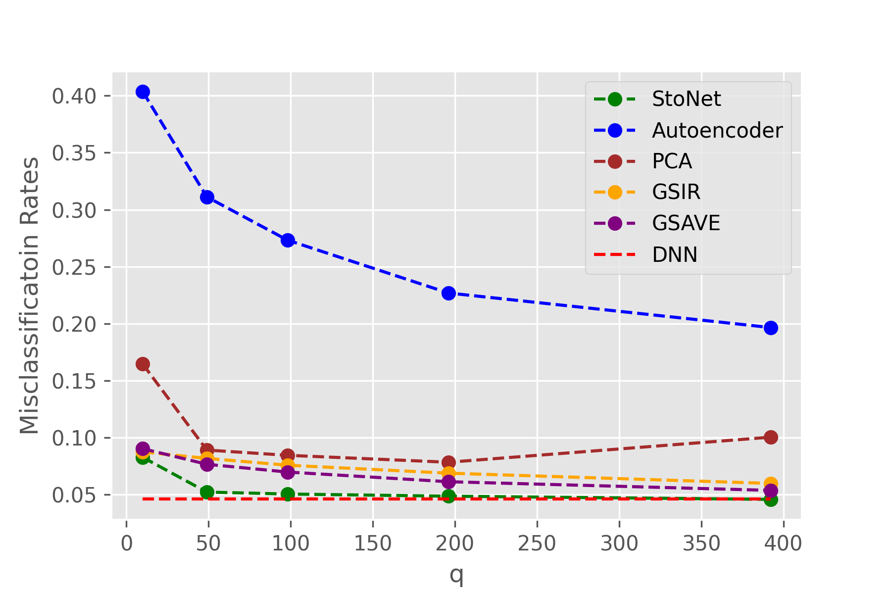
Refer to caption
Figure S1: Misclassification rates versus dimension qq. The red dash line represent the baseline result by training a DNN with one hidden layer and 50 hidden units on the original dataset (mistclassification rate = 0.04590.0459).

The experimental results are summarized in Figure S1 and Table 2 (of the main text). For the dataset, we also trained a DNN with one hidden layer and 50 hidden units as the comparison baseline, which achieved a prediction error rate of 0.0459. The comparison shows that the StoNet outperforms GSIR, GSAVE, autoencoder and PCA in terms of misclassification rates. Moreover, StoNet is much more efficient than GSIR, GSAVE and autoencoder in computational time. It is interesting to note that when the data was projected onto a subspace with dimension 392, StoNet even outperformed the DNN in prediction accuracy. We have also tried LSMIE for this example, but lost interests finally as the method took more than 24 CPU hours on our computer.

S1.2 A Regression Example

Refer to Figure S2 for the performance of different methods on the example.

Refer to caption
Figure S2: Pearson Correlation v.s. dimension qq for the regression example. The red dash line represent the baseline result by training a DNN with one hidden layer and 100 hidden units on the original dataset (Pearson correlation = 0.9987​(0.0000)0.9987(0.0000)).

Appendix S2 Proofs of Theorem 2.1 and Theorem 2.2

S2.1 Proof of Theorem 2.1

Since Θ\Theta is compact, it suffices to prove that the consistency holds for each value of 𝜽{\boldsymbol{\theta}}. For simplicity of notation, we rewrite σn,i\sigma_{n,i} by σi\sigma_{i} in the remaining part of the proof.

Let 𝒀m​i​s=(𝒀1,𝒀2,…,𝒀h){\boldsymbol{Y}}_{mis}=({\boldsymbol{Y}}_{1},{\boldsymbol{Y}}_{2},\dots,{\boldsymbol{Y}}_{h}), where 𝒀i{\boldsymbol{Y}}_{i}’s are latent variables as given in Equation (6) of the main text. Let 𝒀~=(𝒀~1,…,𝒀~h)\boldsymbol{\tilde{Y}}=(\boldsymbol{\tilde{Y}}_{1},\dots,\boldsymbol{\tilde{Y}}_{h}), where 𝒀~i\boldsymbol{\tilde{Y}}_{i}’s are calculated by the neural network in Equation (5) of the main text. By Taylor expansion, we have

logπ(𝒀,𝒀m​i​s|𝑿,𝜽)=logπ(𝒀,𝒀~|𝑿,𝜽)+ϵT∇𝒀m​i​slogπ(𝒀,𝒀~|𝑿,𝜽)+O(∥ϵ∥2),\log\pi({\boldsymbol{Y}},{\boldsymbol{Y}}_{mis}|{\boldsymbol{X}},{\boldsymbol{\theta}})=\log\pi({\boldsymbol{Y}},\tilde{{\boldsymbol{Y}}}|{\boldsymbol{X}},{\boldsymbol{\theta}})+\boldsymbol{\epsilon}^{T}\nabla_{{\boldsymbol{Y}}_{mis}}\log\pi({\boldsymbol{Y}},\tilde{{\boldsymbol{Y}}}|{\boldsymbol{X}},{\boldsymbol{\theta}})+O(\|\boldsymbol{\epsilon}\|^{2}), (S1)

where ϵ=𝒀−𝒀m​i​s=(ϵ1,ϵ2,…,ϵh)\boldsymbol{\epsilon}={\boldsymbol{Y}}-{\boldsymbol{Y}}_{mis}=(\boldsymbol{\epsilon}_{1},\boldsymbol{\epsilon}_{2},\dots,\boldsymbol{\epsilon}_{h}), logπ(𝒀,𝒀~|𝑿,𝜽)=logπ(𝒀|𝑿,𝜽)\log\pi({\boldsymbol{Y}},\tilde{{\boldsymbol{Y}}}|{\boldsymbol{X}},{\boldsymbol{\theta}})=\log\pi({\boldsymbol{Y}}|{\boldsymbol{X}},{\boldsymbol{\theta}}) is the log-likelihood function of the neural network, and ∇𝒀m​i​slogπ(𝒀,𝒀~|𝑿,𝜽)\nabla_{{\boldsymbol{Y}}_{mis}}\log\pi({\boldsymbol{Y}},\tilde{{\boldsymbol{Y}}}|{\boldsymbol{X}},{\boldsymbol{\theta}}) is evaluated according to the joint distribution given in Equation (10) of the main text.

Consider ∇𝒀ilogπ(𝒀,𝒀~i|𝑿,𝜽)\nabla_{{\boldsymbol{Y}}_{i}}\log\pi({\boldsymbol{Y}},\tilde{{\boldsymbol{Y}}}_{i}|{\boldsymbol{X}},{\boldsymbol{\theta}}). For its single latent variable, say Yi(k)Y_{i}^{(k)}, the output of the hidden unit kk at layer i∈{2,…,h}i\in\{2,\dots,h\}, we have

∇Yi(k)logπ(𝒀,Y~i(k)|𝑿,𝜽)=1σi+12​∑j=1di+1(Yi+1(j)−bi+1(j)−𝒘i+1(j)​ψ​(𝒀~i))​wi+1(j,k)​ψ′​(Y~i(k))−1σi2​(Y~i(k)−bi(k)−𝒘i(k)​ψ​(𝒀i−1))\begin{split}\nabla_{Y_{i}^{(k)}}\log\pi({\boldsymbol{Y}},\tilde{Y}_{i}^{(k)}|{\boldsymbol{X}},{\boldsymbol{\theta}})&=\frac{1}{\sigma_{i+1}^{2}}\sum_{j=1}^{d_{i+1}}(Y_{i+1}^{(j)}-b_{i+1}^{(j)}-{\boldsymbol{w}}_{i+1}^{(j)}\psi(\tilde{{\boldsymbol{Y}}}_{i}))w_{i+1}^{(j,k)}\psi^{\prime}(\tilde{Y}_{i}^{(k)})\\ &-\frac{1}{\sigma_{i}^{2}}(\tilde{Y}_{i}^{(k)}-b_{i}^{(k)}-{\boldsymbol{w}}_{i}^{(k)}\psi({\boldsymbol{Y}}_{i-1}))\end{split} (S2)

where 𝒘i+1(j){\boldsymbol{w}}_{i+1}^{(j)} denotes the vector of the weights from hidden unit jj at layer i+1i+1 to the hidden units at layer ii, and wi+1(j,k)w_{i+1}^{(j,k)} denotes the weight from hidden unit jj at layer i+1i+1 to the hidden unit kk at hidden layer ii. Further, by noting that Yi+1(j)=bi+1(j)+𝒘i+1(j)​ψ​(𝒀i)+ei+1(j)Y_{i+1}^{(j)}=b_{i+1}^{(j)}+{\boldsymbol{w}}_{i+1}^{(j)}\psi({\boldsymbol{Y}}_{i})+e_{i+1}^{(j)} and Yi(j)=bi(j)+𝒘i(j)​ψ​(𝒀i−1)Y_{i}^{(j)}=b_{i}^{(j)}+{\boldsymbol{w}}_{i}^{(j)}\psi({\boldsymbol{Y}}_{i-1}), we have

∇Yi(k)logπ(𝒀,Y~i(k)|𝑿,𝜽)=1σi+12​∑j=1di+1(ei+1(j)+𝒘i+1(j)​(ψ⁡(𝒀i)−ψ⁡(𝒀~i)))​wi+1(j,k)​ψ′​(Y~i,k)−1σi2𝒘i(k)[ψ(𝒀~i−1)−ψ(𝒀i−1))].\begin{split}\nabla_{Y_{i}^{(k)}}\log\pi({\boldsymbol{Y}},\tilde{Y}_{i}^{(k)}|{\boldsymbol{X}},{\boldsymbol{\theta}})&=\frac{1}{\sigma_{i+1}^{2}}\sum_{j=1}^{d_{i+1}}(e_{i+1}^{(j)}+{\boldsymbol{w}}_{i+1}^{(j)}(\psi({\boldsymbol{Y}}_{i})-\psi(\tilde{{\boldsymbol{Y}}}_{i})))w_{i+1}^{(j,k)}\psi^{\prime}(\tilde{Y}_{i,k})\\ &-\frac{1}{\sigma_{i}^{2}}{\boldsymbol{w}}_{i}^{(k)}[\psi(\tilde{{\boldsymbol{Y}}}_{i-1})-\psi({\boldsymbol{Y}}_{i-1}))].\end{split} (S3)

For layer i=1i=1, the calculation is similar, but the second term in (S3) is reduced to 00. Then by Assumption 2.1-(i)&(iv), we have

|∇Yi(k)logπ(𝒀,Y~i(k)∣𝑿,𝜽)|≤{1σi+12​{∑j=1mi+1ei+1(j)​wi+1(j,k)​ψ′​(Y~i(k))+(c′​r)2​mi+1​‖ϵi‖}+1σi2​c′​r​‖ϵi−1‖, if ​i>11σi+12​{∑j=1mi+1ei+1(j)​wi+1(j,k)​ψ′​(Y~i(k))+(c′​r)2​mi+1​‖ϵi‖}, if ​i=1\begin{array}[]{l}\left|\nabla_{Y_{i}^{(k)}}\log\pi\left(\boldsymbol{Y},\tilde{Y}_{i}^{(k)}\mid\boldsymbol{X},\boldsymbol{\theta}\right)\right|\\ \leq\left\{\begin{array}[]{ll}\frac{1}{\sigma_{i+1}^{2}}\left\{\sum_{j=1}^{m_{i+1}}e_{i+1}^{(j)}w_{i+1}^{(j,k)}\psi^{\prime}\left(\tilde{Y}_{i}^{(k)}\right)+\left(c^{\prime}r\right)^{2}m_{i+1}\left\|\boldsymbol{\epsilon}_{i}\right\|\right\}+\frac{1}{\sigma_{i}^{2}}c^{\prime}r\left\|\boldsymbol{\epsilon}_{i-1}\right\|,&\text{ if }i>1\\ \frac{1}{\sigma_{i+1}^{2}}\left\{\sum_{j=1}^{m_{i+1}}e_{i+1}^{(j)}w_{i+1}^{(j,k)}\psi^{\prime}\left(\tilde{Y}_{i}^{(k)}\right)+\left(c^{\prime}r\right)^{2}m_{i+1}\left\|\boldsymbol{\epsilon}_{i}\right\|\right\},&\text{ if }i=1\end{array}\right.\end{array} (S4)

Next, let’s figure out the order of ‖ϵi‖\|\boldsymbol{\epsilon}_{i}\|. The kkth component of ϵi\boldsymbol{\epsilon}_{i} is given by

Yi(k)−Y~i(k)={ei(k)+𝒘i(k)​(ψ⁡(𝒀i−1)−ψ⁡(𝒀~i−1)),i>1,ei(k)i=1.Y_{i}^{(k)}-\tilde{Y}_{i}^{(k)}=\left\{\begin{array}[]{lr}e_{i}^{(k)}+{\boldsymbol{w}}_{i}^{(k)}(\psi({\boldsymbol{Y}}_{i-1})-\psi(\tilde{{\boldsymbol{Y}}}_{i-1})),&i>1,\\ e_{i}^{(k)}&i=1.\\ \end{array}\right. (S5)

Therefore, ‖ϵ1‖=‖𝒆1‖\|\boldsymbol{\epsilon}_{1}\|=\|{\boldsymbol{e}}_{1}\|; and for i=2,3,…,hi=2,3,\dots,h, the following inequalities hold:

‖ϵi‖≤‖𝒆i‖+c′​r​di​‖ϵi−1‖,a​n​d‖ϵi‖2≤2​‖𝒆i‖2+2​(c′​r)2​di2​‖ϵi−1‖2.\|\boldsymbol{\epsilon}_{i}\|\leq\|{\boldsymbol{e}}_{i}\|+c^{\prime}rd_{i}\|\boldsymbol{\epsilon}_{i-1}\|,\quad and\quad\|\boldsymbol{\epsilon}_{i}\|^{2}\leq 2\|{\boldsymbol{e}}_{i}\|^{2}+2(c^{\prime}r)^{2}d_{i}^{2}\|\boldsymbol{\epsilon}_{i-1}\|^{2}. (S6)

Since 𝒆i{\boldsymbol{e}}_{i} and 𝒆i−1{\boldsymbol{e}}_{i-1} are independent, by summarizing (S4) and (S6), we have

∫ϵT∇𝒀m​i​slogπ(𝒀,𝒀~|𝑿,𝜽)π(𝒀m​i​s|𝑿,𝜽,𝒀)d𝒀m​i​s≤O(∑k=2h+1σk−12σh+12dh+1(∏i=khdi2)dk−1)+O⁡(∑k=2hσk−12σh2​dh​(∏i=kh−1di2)​dk−1)+⋯+O⁡(σ12σ22​d2​d1)=o⁡(1),\begin{split}&\int\boldsymbol{\epsilon}^{T}\nabla_{{\boldsymbol{Y}}_{mis}}\log\pi(\boldsymbol{Y,\tilde{{\boldsymbol{Y}}}}|{\boldsymbol{X}},{\boldsymbol{\theta}})\pi({\boldsymbol{Y}}_{mis}|{\boldsymbol{X}},{\boldsymbol{\theta}},{\boldsymbol{Y}})d{\boldsymbol{Y}}_{mis}\leq O\left(\sum_{k=2}^{h+1}\frac{\sigma_{k-1}^{2}}{\sigma_{h+1}^{2}}d_{h+1}(\prod_{i=k}^{h}d_{i}^{2})d_{k-1}\right)\\ &+O\left(\sum_{k=2}^{h}\frac{\sigma_{k-1}^{2}}{\sigma_{h}^{2}}d_{h}(\prod_{i=k}^{h-1}d_{i}^{2})d_{k-1}\right)+\dots+O\left(\frac{\sigma_{1}^{2}}{\sigma_{2}^{2}}d_{2}d_{1}\right)=o(1),\end{split} (S7)

which, by (S1) and Assumption 2.1-(v)(v), implies the mean value

𝔼[logπ(𝒀,𝒀m​i​s|𝑿,𝜽)−logπ(𝒀|𝑿,θ)]→0,∀𝜽∈Θ\mathbb{E}[\log\pi({\boldsymbol{Y}},{\boldsymbol{Y}}_{mis}|{\boldsymbol{X}},{\boldsymbol{\theta}})-\log\pi({\boldsymbol{Y}}|{\boldsymbol{X}},\theta)]\rightarrow 0,\quad\forall{\boldsymbol{\theta}}\in\Theta (S8)

Further, it is easy to verify

∫|ϵT∇𝒀m​i​slogπ(𝒀,𝒀~|𝑿,𝜽)|2π(𝒀m​i​s|𝑿,𝜽,𝒀)d𝒀m​i​s<∞,\int|\boldsymbol{\epsilon}^{T}\nabla_{{\boldsymbol{Y}}_{mis}}\log\pi({\boldsymbol{Y}},\tilde{{\boldsymbol{Y}}}|{\boldsymbol{X}},{\boldsymbol{\theta}})|^{2}\pi({\boldsymbol{Y}}_{mis}|{\boldsymbol{X}},{\boldsymbol{\theta}},{\boldsymbol{Y}})d{\boldsymbol{Y}}_{mis}<\infty, (S9)

which, together with (S1) and (S6), implies

𝔼|logπ(𝒀,𝒀m​i​s|𝑿,𝜽)−logπ(𝒀|𝑿,𝜽)|2<∞.\mathbb{E}|\log\pi({\boldsymbol{Y}},{\boldsymbol{Y}}_{mis}|{\boldsymbol{X}},{\boldsymbol{\theta}})-\log\pi({\boldsymbol{Y}}|{\boldsymbol{X}},{\boldsymbol{\theta}})|^{2}<\infty. (S10)

Therefore, the weak law of large numbers (WLLN) applies, and the proof can be concluded. □\Box

S2.2 Proof of Theorem 2.2

To prove Theorem 2.2, we first prove Lemma S1, from which Theorem 2.2 can be directly derived.

Lemma S1

Consider a function Q⁡(𝛉,𝐗n)Q({\boldsymbol{\theta}},{\boldsymbol{X}}_{n}). Suppose that the following conditions are satisfied:

  1. (i)

    Q⁡(𝜽,𝑿n)Q({\boldsymbol{\theta}},{\boldsymbol{X}}_{n}) is continuous in 𝜽{\boldsymbol{\theta}} and there exists a function Q∗​(𝜽)Q^{*}({\boldsymbol{\theta}}), which is continuous in 𝜽{\boldsymbol{\theta}} and uniquely maximized at 𝜽∗{\boldsymbol{\theta}}^{*}.

  2. (ii)

    For any ϵ>0\epsilon>0, sup𝜽∈Θ\B⁡(ϵ)Q∗​(𝜽)\sup_{{\boldsymbol{\theta}}\in\Theta\backslash B(\epsilon)}Q^{*}({\boldsymbol{\theta}}) exists, where B⁡(ϵ)={𝜽:‖𝜽−𝜽∗‖<ϵ}B(\epsilon)=\{\boldsymbol{\theta:\|{\boldsymbol{\theta}}-{\boldsymbol{\theta}}^{*}\|<\epsilon}\}; Let δ=Q∗​(𝜽∗)−sup𝜽∈Θ\B⁡(ϵ)Q∗​(𝜽)\delta=Q^{*}({\boldsymbol{\theta}}^{*})-\sup_{{\boldsymbol{\theta}}\in\Theta\backslash B(\epsilon)}Q^{*}({\boldsymbol{\theta}}).

  3. (iii)

    sup𝜽∈Θ|Q⁡(𝜽,𝑿n)−Q∗​(𝜽)|​→𝑝​0\sup_{{\boldsymbol{\theta}}\in\Theta}|Q({\boldsymbol{\theta}},{\boldsymbol{X}}_{n})-Q^{*}({\boldsymbol{\theta}})|\overset{p}{\rightarrow}0 as n→∞n\rightarrow\infty.

Let θ^n=arg⁡max𝛉∈Θ⁡Q⁡(𝛉,𝐗n)\hat{\theta}_{n}=\arg\max_{{\boldsymbol{\theta}}\in\Theta}Q({\boldsymbol{\theta}},{\boldsymbol{X}}_{n}). Then ‖𝛉^n−𝛉∗‖​→𝑝​0\|\hat{{\boldsymbol{\theta}}}_{n}-{\boldsymbol{\theta}}^{*}\|\overset{p}{\rightarrow}0.

Consider two events:

  1. (a)

    sup𝜽∈Θ\B⁡(ϵ)|Q⁡(𝜽,𝑿n)−Q∗​(𝜽)|<δ/2\sup_{{\boldsymbol{\theta}}\in\Theta\backslash B(\epsilon)}|Q({\boldsymbol{\theta}},{\boldsymbol{X}}_{n})-Q^{*}({\boldsymbol{\theta}})|<\delta/2, and

  2. (b)

    sup𝜽∈Θ|Q⁡(𝜽,𝑿n)−Q∗​(𝜽)|<δ/2\sup_{{\boldsymbol{\theta}}\in\Theta}|Q({\boldsymbol{\theta}},{\boldsymbol{X}}_{n})-Q^{*}({\boldsymbol{\theta}})|<\delta/2.

From event (a), we can deduce that for any 𝜽∈Θ\B⁡(ϵ){\boldsymbol{\theta}}\in\Theta\backslash B(\epsilon), Q⁡(𝜽,𝑿n)<Q∗​(𝜽)+δ/2≤Q∗​(𝜽∗)−δ+δ/2≤Q∗​(𝜽∗)−δ/2Q({\boldsymbol{\theta}},{\boldsymbol{X}}_{n})<Q^{*}({\boldsymbol{\theta}})+\delta/2\leq Q^{*}(\boldsymbol{\theta^{*}})-\delta+\delta/2\leq Q^{*}(\boldsymbol{\theta^{*}})-\delta/2. From event (b), we can deduce that for any 𝜽∈B⁡(ϵ){\boldsymbol{\theta}}\in B(\epsilon), Q⁡(𝜽,𝑿𝒏)>Q∗​(𝜽)−δ/2Q(\boldsymbol{\theta,{\boldsymbol{X}}_{n}})>Q^{*}({\boldsymbol{\theta}})-\delta/2 and thus Q⁡(𝜽∗,𝑿n)>Q∗​(𝜽∗)−δ/2Q({\boldsymbol{\theta}}^{*},{\boldsymbol{X}}_{n})>Q^{*}({\boldsymbol{\theta}}^{*})-\delta/2.

If both events hold simultaneously, then we must have 𝜽^n∈B⁡(ϵ)\hat{{\boldsymbol{\theta}}}_{n}\in B(\epsilon) as n→∞n\rightarrow\infty. By condition (i​i​i)(iii), the probability that both events hold tends to 1. Therefore, P⁡(𝜽^n∈B⁡(ϵ))→1P(\hat{{\boldsymbol{\theta}}}_{n}\in B(\epsilon))\rightarrow 1. □\Box

Appendix S3 Proofs of Theorem 3.1 and Theorem 3.2

Since our goal is to obtain the SDR predictor 𝒀h{\boldsymbol{Y}}_{h} for all observations in 𝑫{\boldsymbol{D}}, we proved the convergence of Algorithm 1 for the case that the full training dataset is used at each iteration. If the algorithm is used for other purposes, say estimation of 𝜽{\boldsymbol{\theta}} only, a mini-batch of data can be used at each iteration. Extension of our proof for the mini-batch case will be discussed in Remark S2. To complete the proof, we make the following assumptions.

Assumption B1

The function F𝐃​(⋅,⋅)F_{{\boldsymbol{D}}}(\cdot,\cdot) takes nonnegative real values, and there exist constants A,B≥0A,B\geq 0, such that |F𝐃​(𝟎,𝛉∗)|≤A|F_{{\boldsymbol{D}}}(\boldsymbol{0},{\boldsymbol{\theta}}^{*})|\leq A, ‖∇𝐙F𝐃​(𝟎,𝛉∗)‖≤B\|\nabla_{{\boldsymbol{Z}}}F_{{\boldsymbol{D}}}(\boldsymbol{0},{\boldsymbol{\theta}}^{*})\|\leq B, ‖∇𝛉F𝐃​(𝟎,𝛉∗)‖≤B\|\nabla_{{\boldsymbol{\theta}}}F_{{\boldsymbol{D}}}(\boldsymbol{0},{\boldsymbol{\theta}}^{*})\|\leq B, and ‖H⁡(𝟎,𝛉∗)‖≤B\|H(\boldsymbol{0},{\boldsymbol{\theta}}^{*})\|\leq B.

Assumption B2

(Smoothness) F𝐃​(⋅,⋅)F_{{\boldsymbol{D}}}(\cdot,\cdot) is MM-smooth and H⁡(⋅,⋅)H(\cdot,\cdot) is MM-Lipschitz: there exists some constant M>0M>0 such that for any 𝐙,𝐙′∈ℝdz{\boldsymbol{Z}},{\boldsymbol{Z}}^{\prime}\in\mathbb{R}^{d_{z}} and any 𝛉,𝛉′∈Θ{\boldsymbol{\theta}},{\boldsymbol{\theta}}^{\prime}\in\Theta,

‖∇𝒁F𝑫​(𝒁,𝜽)−∇𝒁F𝑫​(𝒁′,𝜽′)‖≤M|𝒁−𝒁′|+M​‖𝜽−𝜽′‖,‖∇𝜽F𝑫​(𝒁,𝜽)−∇𝜽F𝑫​(𝒁′,𝜽′)‖≤M|𝒁−𝒁′|+M​‖𝜽−𝜽′‖,‖H⁡(𝒁,𝜽)−H⁡(𝒁′,𝜽′)‖≤M|𝒁−𝒁′|+M​‖𝜽−𝜽′‖.\begin{split}&\|\nabla_{{\boldsymbol{Z}}}F_{{\boldsymbol{D}}}({\boldsymbol{Z}},{\boldsymbol{\theta}})-\nabla_{{\boldsymbol{Z}}}F_{{\boldsymbol{D}}}({\boldsymbol{Z}}^{\prime},{\boldsymbol{\theta}}^{\prime})\|\leq M\|{\boldsymbol{Z}}-{\boldsymbol{Z}}^{\prime}\|+M\|{\boldsymbol{\theta}}-{\boldsymbol{\theta}}^{\prime}\|,\\ &\|\nabla_{{\boldsymbol{\theta}}}F_{{\boldsymbol{D}}}({\boldsymbol{Z}},{\boldsymbol{\theta}})-\nabla_{{\boldsymbol{\theta}}}F_{{\boldsymbol{D}}}({\boldsymbol{Z}}^{\prime},{\boldsymbol{\theta}}^{\prime})\|\leq M\|{\boldsymbol{Z}}-{\boldsymbol{Z}}^{\prime}\|+M\|{\boldsymbol{\theta}}-{\boldsymbol{\theta}}^{\prime}\|,\\ &{\color[rgb]{0,0,0}\|H({\boldsymbol{Z}},{\boldsymbol{\theta}})-H({\boldsymbol{Z}}^{\prime},{\boldsymbol{\theta}}^{\prime})\|\leq M\|{\boldsymbol{Z}}-{\boldsymbol{Z}}^{\prime}\|+M\|{\boldsymbol{\theta}}-{\boldsymbol{\theta}}^{\prime}\|}.\end{split}
Assumption B3

(Dissipativity) For any 𝛉∈Θ{\boldsymbol{\theta}}\in\Theta, the function F𝐃​(⋅,𝛉∗)F_{{\boldsymbol{D}}}(\cdot,{\boldsymbol{\theta}}^{*}) is (m,b)(m,b)-dissipative: there exist some constants m>12m>\frac{1}{2} and b≥0b\geq 0 such that ⟨𝐙,∇𝐙F𝐃​(𝐙,𝛉∗)⟩≥m​‖𝐙‖2−b\langle{\boldsymbol{Z}},\nabla_{{\boldsymbol{Z}}}F_{{\boldsymbol{D}}}({\boldsymbol{Z}},{\boldsymbol{\theta}}^{*})\rangle\geq m\|{\boldsymbol{Z}}\|^{2}-b.

The smoothness and dissipativity conditions are regular for studying the convergence of stochastic gradient MCMC algorithms, and they have been used in many papers such as [41] and [17]. As implied by the definition of F𝑫​(𝒁,𝜽)F_{{\boldsymbol{D}}}({\boldsymbol{Z}},{\boldsymbol{\theta}}), the values of MM, mm and bb increase linearly with the sample size nn. Therefore, we can impose a nonzero lower bound on mm to facilitate the proof of Lemma S1.

Assumption B4

(Gradient noise) There exists a constant ς∈[0,1)\varsigma\in[0,1) such that for any 𝐙{\boldsymbol{Z}} and 𝛉{\boldsymbol{\theta}}, 𝔼​‖∇𝐙F^𝐃​(𝐙,𝛉)−∇𝐙F𝐃​(𝐙,𝛉)‖2≤2​ς​(M2​‖𝐙‖2+M2​‖𝛉−𝛉∗‖2+B2)\mathbb{E}\|\nabla_{{\boldsymbol{Z}}}\hat{F}_{{\boldsymbol{D}}}({\boldsymbol{Z}},{\boldsymbol{\theta}})-\nabla_{{\boldsymbol{Z}}}F_{{\boldsymbol{D}}}({\boldsymbol{Z}},{\boldsymbol{\theta}})\|^{2}\leq 2\varsigma(M^{2}\|{\boldsymbol{Z}}\|^{2}+M^{2}\|{\boldsymbol{\theta}}-{\boldsymbol{\theta}}^{*}\|^{2}+B^{2}).

Introduction of the extra constant ς\varsigma facilitates our study. For the full data case, we have ς=0\varsigma=0, i.e., the gradient ∇𝒁F𝑫​(𝒁,𝜽)\nabla_{{\boldsymbol{Z}}}F_{{\boldsymbol{D}}}({\boldsymbol{Z}},{\boldsymbol{\theta}}) can be evaluated accurately.

Assumption B5

The step size {γk}k∈ℕ\{\gamma_{k}\}_{k\in\mathbb{N}} is a positive decreasing sequence such that γk→0\gamma_{k}\rightarrow 0 and ∑k=1∞γk=∞\sum_{k=1}^{\infty}\gamma_{k}=\infty. In addition, let h⁡(𝛉)=𝔼⁡(H⁡(𝐙,𝛉))h({\boldsymbol{\theta}})=\mathbb{E}(H({\boldsymbol{Z}},{\boldsymbol{\theta}})), then there exists δ>0\delta>0 such that for any 𝛉∈Θ{\boldsymbol{\theta}}\in\Theta, ⟨𝛉−𝛉∗,h(𝛉))⟩≥δ∥𝛉−𝛉∗∥2\langle{\boldsymbol{\theta}}-{\boldsymbol{\theta}}^{*},h({\boldsymbol{\theta}}))\rangle\geq\delta\|{\boldsymbol{\theta}}-{\boldsymbol{\theta}}^{*}\|^{2}, and lim infk→∞2​δ​γkγk+1+γk+1−γkγk+12>0\liminf_{k\rightarrow\infty}2\delta\frac{\gamma_{k}}{\gamma_{k+1}}+\frac{\gamma_{k+1}-\gamma_{k}}{\gamma_{k+1}^{2}}>0.

As shown by [4] (p.244), Assumption B5 can be satisfied by setting γk=a~/(b~+kα)\gamma_{k}=\tilde{a}/(\tilde{b}+k^{\alpha}) for some constants a~>0\tilde{a}>0, b~≥0\tilde{b}\geq 0, and α∈(0,1∧2​δ​a~)\alpha\in(0,1\wedge 2\delta\tilde{a}). By (17), δ\delta increases linearly with the sample size nn. Therefore, if we set a~=Ω⁡(1/n)\tilde{a}=\Omega(1/n) then 2​δ​a~>12\delta\tilde{a}>1 can be satisfied, where Ω⁡(⋅)\Omega(\cdot) denotes the order of the lower bound of a function. In this paper, we simply choose α∈(0,1)\alpha\in(0,1) by assuming that a~\tilde{a} has been set appropriately with 2​δ​a~≥12\delta\tilde{a}\geq 1 held.

Assumption B6

(Solution of Poisson equation) For any 𝛉∈Θ{\boldsymbol{\theta}}\in\Theta, 𝐳∈ℨ{\boldsymbol{z}}\in\mathfrak{Z}, and a function V⁡(𝐳)=1+‖𝐳‖V({\boldsymbol{z}})=1+\|{\boldsymbol{z}}\|, there exists a function μ𝛉\mu_{{\boldsymbol{\theta}}} on ℨ\mathfrak{Z} that solves the Poisson equation μ𝛉​(𝐳)−𝒯𝛉​μ𝛉​(𝐳)=H⁡(𝛉,𝐳)−h⁡(𝛉)\mu_{{\boldsymbol{\theta}}}({\boldsymbol{z}})-\mathcal{T}_{{\boldsymbol{\theta}}}\mu_{{\boldsymbol{\theta}}}({\boldsymbol{z}})={H}({\boldsymbol{\theta}},{\boldsymbol{z}})-h({\boldsymbol{\theta}}), where 𝒯𝛉\mathcal{T}_{{\boldsymbol{\theta}}} denotes a probability transition kernel with 𝒯𝛉​μ𝛉​(𝐳)=∫ℨμ𝛉​(𝐳′)​𝒯𝛉​(𝐳,𝐳′)​d​𝐳′\mathcal{T}_{{\boldsymbol{\theta}}}\mu_{{\boldsymbol{\theta}}}({\boldsymbol{z}})=\int_{\mathfrak{Z}}\mu_{{\boldsymbol{\theta}}}({\boldsymbol{z}}^{\prime})\mathcal{T}_{{\boldsymbol{\theta}}}({\boldsymbol{z}},{\boldsymbol{z}}^{\prime})d{\boldsymbol{z}}^{\prime}, such that

H(𝜽k,𝒛k+1)=h(𝜽k)+μ𝜽k(𝒛k+1)−𝒯𝜽kμ𝜽k(𝒛k+1),k=1,2,….{H}({\boldsymbol{\theta}}_{k},{\boldsymbol{z}}_{k+1})=h({\boldsymbol{\theta}}_{k})+\mu_{{\boldsymbol{\theta}}_{k}}({\boldsymbol{z}}_{k+1})-\mathcal{T}_{{\boldsymbol{\theta}}_{k}}\mu_{{\boldsymbol{\theta}}_{k}}({\boldsymbol{z}}_{k+1}),\quad k=1,2,\ldots. (S11)

Moreover, for all 𝛉,𝛉′∈Θ{\boldsymbol{\theta}},{\boldsymbol{\theta}}^{\prime}\in\Theta and 𝐳∈ℨ{\boldsymbol{z}}\in\mathfrak{Z}, we have ‖μ𝛉​(𝐳)−μ𝛉′​(𝐳)‖≤ς1​‖𝛉−𝛉′‖​V​(𝐳)\|\mu_{{\boldsymbol{\theta}}}({\boldsymbol{z}})-\mu_{{\boldsymbol{\theta}}^{\prime}}({\boldsymbol{z}})\|\leq\varsigma_{1}\|{\boldsymbol{\theta}}-{\boldsymbol{\theta}}^{\prime}\|V({\boldsymbol{z}}) and ‖μ𝛉​(𝐳)‖≤ς2​V​(𝐳)\|\mu_{{\boldsymbol{\theta}}}({\boldsymbol{z}})\|\leq\varsigma_{2}V({\boldsymbol{z}}) for some constants ς1>0\varsigma_{1}>0 and ς2>0\varsigma_{2}>0.

This assumption is also regular for studying the convergence of stochastic gradient MCMC algorithms, see e.g., [48] and [12]. Alternatively, one can assume that the MCMC algorithms satisfy the drift condition, and then Assumption B6 can be verified, see e.g., [2].

S3.1 Proof of Theorem 3.1

Theorem S1 concerns the convergence of 𝜽(k){\boldsymbol{\theta}}^{(k)}, which is a complete version of Theorem 3.1.

Theorem S1

(A complete version of Theorem 3.1) Suppose Assumptions B1-B6 hold. If we set ϵk=Cϵ/(ce+kα)\epsilon_{k}=C_{\epsilon}/(c_{e}+k^{\alpha}) and γk=Cγ/(cg+kα)\gamma_{k}=C_{\gamma}/(c_{g}+k^{\alpha}) for some constants α∈(0,1)\alpha\in(0,1), Cϵ>0C_{\epsilon}>0, Cγ>0C_{\gamma}>0, ce≥0c_{e}\geq 0 and cg≥0c_{g}\geq 0, then there exists an iteration k0k_{0} and a constant λ0>0\lambda_{0}>0 such that for any k>k0k>k_{0},

𝔼⁡(‖𝜽(k)−𝜽∗‖2)≤λ0​γk,\mathbb{E}(\|{\boldsymbol{\theta}}^{(k)}-{\boldsymbol{\theta}}^{*}\|^{2})\leq\lambda_{0}\gamma_{k}, (S12)

where λ0=λ0′+6​6​C𝛉12​((3​M2+ζ2)​C𝐙+3​M2​C𝛉+3​B2+ζ22)12\lambda_{0}=\lambda_{0}^{\prime}+6\sqrt{6}C_{{\boldsymbol{\theta}}}^{\frac{1}{2}}((3M^{2}+\zeta_{2})C_{{\boldsymbol{Z}}}+3M^{2}C_{{\boldsymbol{\theta}}}+3B^{2}+\zeta_{2}^{2})^{\frac{1}{2}} for some constants λ0′\lambda_{0}^{\prime}, C𝛉C_{{\boldsymbol{\theta}}} and C𝐙C_{{\boldsymbol{Z}}}.

Our proof of Theorem 3.1 follows that of Theorem 1 in [12]. However, since Algorithm 1 employs SGHMC for updating 𝒁(k){\boldsymbol{Z}}^{(k)}, which is mathematically very different from the SGLD rule employed in [12], Lemma 1 of [12] (uniform L2L_{2} bounds of 𝜽(k){\boldsymbol{\theta}}^{(k)} and 𝒁(k){\boldsymbol{Z}}^{(k)}) cannot be applied any more. In Lemma S1 below, we prove that 𝔼​‖𝜽(k)‖2≤C𝜽\mathbb{E}\|{\boldsymbol{\theta}}^{(k)}\|^{2}\leq C_{{\boldsymbol{\theta}}}, 𝔼​‖𝒗(k)‖2≤C𝒗\mathbb{E}\|{\boldsymbol{v}}^{(k)}\|^{2}\leq C_{{\boldsymbol{v}}} and 𝔼​‖𝒁(k)‖2≤C𝒁\mathbb{E}\|{\boldsymbol{Z}}^{(k)}\|^{2}\leq C_{{\boldsymbol{Z}}} under appropriate conditions of {ϵk}\{\epsilon_{k}\} and {γk}\{\gamma_{k}\}, where C𝜽C_{{\boldsymbol{\theta}}}, C𝒗C_{{\boldsymbol{v}}} and C𝒁C_{{\boldsymbol{Z}}} are appropriate constants.

Further, based on the proof of [12], we can derive an explicit formula for λ0\lambda_{0}:

λ0=λ0′+6​6​C𝜽12​((3​M2+ζ2)​C𝒁+3​M2​C𝜽+3​B2+ζ22)12,\lambda_{0}=\lambda_{0}^{\prime}+6\sqrt{6}C_{{\boldsymbol{\theta}}}^{\frac{1}{2}}((3M^{2}+\zeta_{2})C_{{\boldsymbol{Z}}}+3M^{2}C_{{\boldsymbol{\theta}}}+3B^{2}+\zeta_{2}^{2})^{\frac{1}{2}},

where λ0′\lambda_{0}^{\prime} together with k0k_{0} can be derived from Lemma 3 of [12] and they depend on δ\delta and {γk}\{\gamma_{k}\} only. The second term of λ0\lambda_{0} is obtained by applying the Cauchy-Schwarz inequality to bound the expectation E⁡⟨𝜽(k)−𝜽∗,𝒯𝜽k−1​μ𝜽k−1​(𝒁(k))⟩E\langle{\boldsymbol{\theta}}^{(k)}-{\boldsymbol{\theta}}^{*},\mathcal{T}_{{\boldsymbol{\theta}}_{k-1}}\mu_{{\boldsymbol{\theta}}_{k-1}}({\boldsymbol{Z}}^{(k)})\rangle, where E​‖𝜽(k)−𝜽∗‖2E\|{\boldsymbol{\theta}}^{(k)}-{\boldsymbol{\theta}}^{*}\|^{2} can be bounded according to Lemma S1 and E​‖𝒯𝜽(k−1)​μ𝜽(k−1)​(𝒁(k))‖2E\|\mathcal{T}_{{\boldsymbol{\theta}}^{(k-1)}}\mu_{{\boldsymbol{\theta}}^{(k-1)}}({\boldsymbol{Z}}^{(k)})\|^{2} can be bounded according to equation (18) of Assumption B6 and the upper bound of H⁡(𝒛,𝜽)H({\boldsymbol{z}},{\boldsymbol{\theta}}) given in (S13). □\Box

Lemma S1

(L2L_{2}-bound) Suppose Assumptions 3.1-3.5 hold. If we set ϵk=Cϵ/(ce+kα)\epsilon_{k}=C_{\epsilon}/(c_{e}+k^{\alpha}) and γk=Cγ/(cg+kα)\gamma_{k}=C_{\gamma}/(c_{g}+k^{\alpha}) for some constants α∈(0,1]\alpha\in(0,1], Cϵ>0C_{\epsilon}>0, Cγ>0C_{\gamma}>0, ce≥0c_{e}\geq 0 and cg≥0c_{g}\geq 0, then there exist constants C𝐯C_{{\boldsymbol{v}}}, C𝐙C_{{\boldsymbol{Z}}} and C𝛉C_{{\boldsymbol{\theta}}} such that supi≥0𝔼​‖𝐯(i)‖2≤C𝐯\sup_{i\geq 0}\mathbb{E}\left\|{\boldsymbol{v}}^{(i)}\right\|^{2}\leq C_{{\boldsymbol{v}}}, supi≥0𝔼​‖𝐙(i)‖2≤C𝐙\sup_{i\geq 0}\mathbb{E}\left\|{\boldsymbol{Z}}^{(i)}\right\|^{2}\leq C_{{\boldsymbol{Z}}}, and supi≥0𝔼​‖𝛉(i)‖2≤C𝛉\sup_{i\geq 0}\mathbb{E}\left\|{\boldsymbol{\theta}}^{(i)}\right\|^{2}\leq C_{{\boldsymbol{\theta}}}.

Similar to the proof of Lemma 1 of [12], we first show

‖∇𝒁F𝑫​(𝒁,𝜽)‖2≤3​M2​‖𝒁‖2+3​M2​‖𝜽−𝜽∗‖2+3​B2,‖∇𝜽F𝑫​(𝒁,𝜽)‖2≤3​M2​‖𝒁‖2+3​M2​‖𝜽−𝜽∗‖2+3​B2,‖H⁡(𝒁(k+1),𝜽(k))‖2≤3​M2​‖𝒁(k+1)‖2+3​M2​‖𝜽(k)−𝜽∗‖2+3​B2.\begin{split}&\|\nabla_{{\boldsymbol{Z}}}F_{{\boldsymbol{D}}}({\boldsymbol{Z}},{\boldsymbol{\theta}})\|^{2}\leq 3M^{2}\|{\boldsymbol{Z}}\|^{2}+3M^{2}\|{\boldsymbol{\theta}}-{\boldsymbol{\theta}}^{*}\|^{2}+3B^{2},\\ &\|\nabla_{{\boldsymbol{\theta}}}F_{{\boldsymbol{D}}}({\boldsymbol{Z}},{\boldsymbol{\theta}})\|^{2}\leq 3M^{2}\|{\boldsymbol{Z}}\|^{2}+3M^{2}\|{\boldsymbol{\theta}}-{\boldsymbol{\theta}}^{*}\|^{2}+3B^{2},\\ &\|H({\boldsymbol{Z}}^{(k+1)},{\boldsymbol{\theta}}^{(k)})\|^{2}\leq 3M^{2}\|{\boldsymbol{Z}}^{(k+1)}\|^{2}+3M^{2}\|{\boldsymbol{\theta}}^{(k)}-{\boldsymbol{\theta}}^{*}\|^{2}+3B^{2}.\end{split} (S13)

By Assumption 3.1, we have ‖∇𝒁F𝑫​(𝟎,𝜽∗)‖≤B,‖H⁡(𝟎,𝜽∗)‖≤B\|\nabla_{{\boldsymbol{Z}}}F_{{\boldsymbol{D}}}(\boldsymbol{0},{\boldsymbol{\theta}}^{*})\|\leq B,\|H(\boldsymbol{0},{\boldsymbol{\theta}}^{*})\|\leq B, and ‖∇𝜽F𝑫​(𝟎,𝜽∗)‖≤B\|\nabla_{{\boldsymbol{\theta}}}F_{{\boldsymbol{D}}}(\boldsymbol{0},{\boldsymbol{\theta}}^{*})\|\leq B. By Assumption 3.2,

‖∇𝒁F𝑫​(𝒁,𝜽)‖≤‖∇𝒁F𝑫​(𝟎,𝜽∗)‖+|∇𝒁F𝑫​(𝒁,𝜽∗)−∇𝒁F𝑫​(𝟎,𝜽∗)|+‖∇𝒁F𝑫​(𝒁,𝜽)−∇𝒁F𝑫​(𝒁,𝜽∗)‖≤B+M​‖𝒁‖+M​‖𝜽−𝜽∗‖,\begin{split}&\|\nabla_{{\boldsymbol{Z}}}F_{{\boldsymbol{D}}}({\boldsymbol{Z}},{\boldsymbol{\theta}})\|\\ \leq&\|\nabla_{{\boldsymbol{Z}}}F_{{\boldsymbol{D}}}(\boldsymbol{0},{\boldsymbol{\theta}}^{*})\|+\|\nabla_{{\boldsymbol{Z}}}F_{{\boldsymbol{D}}}({\boldsymbol{Z}},{\boldsymbol{\theta}}^{*})-\nabla_{{\boldsymbol{Z}}}F_{{\boldsymbol{D}}}(\boldsymbol{0},{\boldsymbol{\theta}}^{*})\|+\|\nabla_{{\boldsymbol{Z}}}F_{{\boldsymbol{D}}}({\boldsymbol{Z}},{\boldsymbol{\theta}})-\nabla_{{\boldsymbol{Z}}}F_{{\boldsymbol{D}}}({\boldsymbol{Z}},{\boldsymbol{\theta}}^{*})\|\\ \leq&B+M\|{\boldsymbol{Z}}\|+M\|{\boldsymbol{\theta}}-{\boldsymbol{\theta}}^{*}\|,\end{split}
‖∇𝜽F𝑫​(𝒁,𝜽)‖≤‖∇𝜽F𝑫​(𝟎,𝜽∗)‖+|∇𝜽F𝑫​(𝒁,𝜽∗)−∇𝜽F𝑫​(𝟎,𝜽∗)|+‖∇𝜽F𝑫​(𝒁,𝜽)−∇𝒁F𝜽​(𝒁,𝜽∗)‖≤B+M​‖𝒁‖+M​‖𝜽−𝜽∗‖,\begin{split}&\|\nabla_{{\boldsymbol{\theta}}}F_{{\boldsymbol{D}}}({\boldsymbol{Z}},{\boldsymbol{\theta}})\|\\ \leq&\|\nabla_{{\boldsymbol{\theta}}}F_{{\boldsymbol{D}}}(\boldsymbol{0},{\boldsymbol{\theta}}^{*})\|+\|\nabla_{{\boldsymbol{\theta}}}F_{{\boldsymbol{D}}}({\boldsymbol{Z}},{\boldsymbol{\theta}}^{*})-\nabla_{{\boldsymbol{\theta}}}F_{{\boldsymbol{D}}}(\boldsymbol{0},{\boldsymbol{\theta}}^{*})\|+\|\nabla_{{\boldsymbol{\theta}}}F_{{\boldsymbol{D}}}({\boldsymbol{Z}},{\boldsymbol{\theta}})-\nabla_{{\boldsymbol{Z}}}F_{{\boldsymbol{\theta}}}({\boldsymbol{Z}},{\boldsymbol{\theta}}^{*})\|\\ \leq&B+M\|{\boldsymbol{Z}}\|+M\|{\boldsymbol{\theta}}-{\boldsymbol{\theta}}^{*}\|,\end{split}
‖H⁡(𝒁(k+1),𝜽(k))‖≤‖H⁡(𝟎,𝜽∗)​‖+‖H⁡(𝒁(k+1),𝜽∗)−H⁡(𝟎,𝜽∗)‖+‖​H​(𝒁(k+1),𝜽(k))−H⁡(𝒁(k+1),𝜽∗)‖≤B+M​‖𝒁(k+1)‖+M​‖𝜽(k)−𝜽∗‖.\begin{split}&\|H({\boldsymbol{Z}}^{(k+1)},{\boldsymbol{\theta}}^{(k)})\|\\ \leq&\|H(\boldsymbol{0},{\boldsymbol{\theta}}^{*})\|+\|H({\boldsymbol{Z}}^{(k+1)},{\boldsymbol{\theta}}^{*})-H(\boldsymbol{0},{\boldsymbol{\theta}}^{*})\|+\|H({\boldsymbol{Z}}^{(k+1)},{\boldsymbol{\theta}}^{(k)})-H({\boldsymbol{Z}}^{(k+1)},{\boldsymbol{\theta}}^{*})\|\\ \leq&B+M\|{\boldsymbol{Z}}^{(k+1)}\|+M\|{\boldsymbol{\theta}}^{(k)}-{\boldsymbol{\theta}}^{*}\|.\end{split}

Therefore, (S13) holds.

By Assumptions 3.2, 3.3 and 2.1-(i), we have

⟨𝒁,∇𝒁F𝑫​(𝒁,𝜽)⟩=⟨𝒁,∇𝒁F𝑫​(𝒁,𝜽∗)⟩−⟨𝒁,∇𝒁F𝑫​(𝒁,𝜽∗)−∇𝒁F𝑫​(𝒁,𝜽)⟩≥m​‖𝒁‖2−b−12​‖𝒁‖2−12​‖∇𝒁F𝑫​(𝒁,𝜽∗)−∇𝒁F𝑫​(𝒁,𝜽)‖2≥(m−12)​‖𝒁‖2−b−12​M2​‖𝜽−𝜽∗‖2≥m0​‖𝒁‖2−b−12​M2​‖𝜽−𝜽∗‖2,\begin{split}\langle{\boldsymbol{Z}},\nabla_{{\boldsymbol{Z}}}F_{{\boldsymbol{D}}}({\boldsymbol{Z}},{\boldsymbol{\theta}})\rangle=&\langle{\boldsymbol{Z}},\nabla_{{\boldsymbol{Z}}}F_{{\boldsymbol{D}}}({\boldsymbol{Z}},{\boldsymbol{\theta}}^{*})\rangle-\langle{\boldsymbol{Z}},\nabla_{{\boldsymbol{Z}}}F_{{\boldsymbol{D}}}({\boldsymbol{Z}},{\boldsymbol{\theta}}^{*})-\nabla_{{\boldsymbol{Z}}}F_{{\boldsymbol{D}}}({\boldsymbol{Z}},{\boldsymbol{\theta}})\rangle\\ \geq&m\|{\boldsymbol{Z}}\|^{2}-b-\frac{1}{2}\|{\boldsymbol{Z}}\|^{2}-\frac{1}{2}\|\nabla_{{\boldsymbol{Z}}}F_{{\boldsymbol{D}}}({\boldsymbol{Z}},{\boldsymbol{\theta}}^{*})-\nabla_{{\boldsymbol{Z}}}F_{{\boldsymbol{D}}}({\boldsymbol{Z}},{\boldsymbol{\theta}})\|^{2}\\ \geq&(m-\frac{1}{2})\|{\boldsymbol{Z}}\|^{2}-b-\frac{1}{2}M^{2}\|{\boldsymbol{\theta}}-{\boldsymbol{\theta}}^{*}\|^{2}\\ {\color[rgb]{0,0,0}\geq}&{\color[rgb]{0,0,0}m_{0}\|{\boldsymbol{Z}}\|^{2}-b-\frac{1}{2}M^{2}\|{\boldsymbol{\theta}}-{\boldsymbol{\theta}}^{*}\|^{2}},\end{split}

where the constants m0=m−12>0m_{0}=m-\frac{1}{2}>0, Then, similar to the proof of Lemma 2 in [41], we have

F𝑫​(𝒁,𝜽)=F𝑫​(𝟎,𝜽∗)+∫01⟨𝒁,∇𝒁F𝑫​(t​𝒁,𝜽∗+t⁡(𝜽−𝜽∗))⟩+⟨𝜽−𝜽∗,∇𝜽F𝑫​(t​𝒁,𝜽∗+t⁡(𝜽−𝜽∗))⟩​𝑑t≤A+∫01‖𝒁‖​‖∇𝒁F𝑫​(t​𝒁,𝜽∗+t⁡(𝜽−𝜽∗))​‖𝑑t+∫01‖𝜽−𝜽∗‖‖​∇𝜽F𝑫​(t​𝒁,𝜽∗+t⁡(𝜽−𝜽∗))‖​𝑑t≤A+‖𝒁‖​∫01t​M​‖𝒁‖+t​M​‖𝜽−𝜽∗‖+B​𝑑t+‖𝜽−𝜽∗‖​∫01t​M|𝒁​‖+t​M‖​𝜽−𝜽∗|+B​𝑑t≤A+M​‖𝒁‖2+M​‖𝜽−𝜽∗‖2+B2​‖𝒁‖2+B2​‖𝜽−𝜽∗‖2+B≤M0​‖𝒁‖2+A0+M0​‖𝜽−𝜽∗‖2,\begin{split}F_{{\boldsymbol{D}}}({\boldsymbol{Z}},{\boldsymbol{\theta}})&=F_{{\boldsymbol{D}}}({\bf 0},{\boldsymbol{\theta}}^{*})+\int_{0}^{1}\langle{\boldsymbol{Z}},\nabla_{{\boldsymbol{Z}}}F_{{\boldsymbol{D}}}(t{\boldsymbol{Z}},{\boldsymbol{\theta}}^{*}+t({\boldsymbol{\theta}}-{\boldsymbol{\theta}}^{*}))\rangle+\langle{\boldsymbol{\theta}}-{\boldsymbol{\theta}}^{*},\nabla_{{\boldsymbol{\theta}}}F_{{\boldsymbol{D}}}(t{\boldsymbol{Z}},{\boldsymbol{\theta}}^{*}+t({\boldsymbol{\theta}}-{\boldsymbol{\theta}}^{*}))\rangle dt\\ &\leq A+\int_{0}^{1}\|{\boldsymbol{Z}}\|\|\nabla_{{\boldsymbol{Z}}}F_{{\boldsymbol{D}}}(t{\boldsymbol{Z}},{\boldsymbol{\theta}}^{*}+t({\boldsymbol{\theta}}-{\boldsymbol{\theta}}^{*}))\|dt+\int_{0}^{1}\|{\boldsymbol{\theta}}-{\boldsymbol{\theta}}^{*}\|\|\nabla_{{\boldsymbol{\theta}}}F_{{\boldsymbol{D}}}(t{\boldsymbol{Z}},{\boldsymbol{\theta}}^{*}+t({\boldsymbol{\theta}}-{\boldsymbol{\theta}}^{*}))\|dt\\ &\leq A+\|{\boldsymbol{Z}}\|\int_{0}^{1}tM\|{\boldsymbol{Z}}\|+tM\|{\boldsymbol{\theta}}-{\boldsymbol{\theta}}^{*}\|+Bdt+\|{\boldsymbol{\theta}}-{\boldsymbol{\theta}}^{*}\|\int_{0}^{1}tM\|{\boldsymbol{Z}}\|+tM\|{\boldsymbol{\theta}}-{\boldsymbol{\theta}}^{*}\|+Bdt\\ &\leq A+M\|{\boldsymbol{Z}}\|^{2}+M\|{\boldsymbol{\theta}}-{\boldsymbol{\theta}}^{*}\|^{2}+\frac{B}{2}\|{\boldsymbol{Z}}\|^{2}+\frac{B}{2}\|{\boldsymbol{\theta}}-{\boldsymbol{\theta}}^{*}\|^{2}+B\\ &{\color[rgb]{0,0,0}\leq M_{0}\|{\boldsymbol{Z}}\|^{2}+A_{0}+M_{0}\|{\boldsymbol{\theta}}-{\boldsymbol{\theta}}^{*}\|^{2}},\end{split}

where the constants M0=M+B2M_{0}=M+\frac{B}{2}, and A0=A+BA_{0}=A+B. Then, similar to [17], for 0<λ<min⁡{14,m02​M0+η2/2}0<\lambda<\min\{\frac{1}{4},\frac{m_{0}}{2M_{0}+\eta^{2}/2}\}, Assumption 3.3 gives us

⟨𝒁,∇𝒁F𝑫​(𝒁,𝜽)⟩≥m0​‖𝒁‖2−b−12​M2​‖𝜽−𝜽∗‖2≥λ⁡(2​M0+η22)​‖𝒁‖2−b−12​M2​‖𝜽−𝜽∗‖2≥2​λ​(F𝑫​(𝒁,𝜽)+η24​‖𝒁‖2)−A1β−(12​M2+2​λ​M0)​‖𝜽−𝜽∗‖2,\begin{split}\langle{\boldsymbol{Z}},\nabla_{{\boldsymbol{Z}}}F_{{\boldsymbol{D}}}({\boldsymbol{Z}},{\boldsymbol{\theta}})\rangle\geq&m_{0}\|{\boldsymbol{Z}}\|^{2}-b-\frac{1}{2}M^{2}\|{\boldsymbol{\theta}}-{\boldsymbol{\theta}}^{*}\|^{2}\geq\lambda(2M_{0}+\frac{\eta^{2}}{2})\|{\boldsymbol{Z}}\|^{2}-b-\frac{1}{2}M^{2}\|{\boldsymbol{\theta}}-{\boldsymbol{\theta}}^{*}\|^{2}\\ \geq&2\lambda(F_{{\boldsymbol{D}}}({\boldsymbol{Z}},{\boldsymbol{\theta}})+\frac{\eta^{2}}{4}\|{\boldsymbol{Z}}\|^{2})-\frac{A_{1}}{\beta}-(\frac{1}{2}M^{2}+2\lambda M_{0})\|{\boldsymbol{\theta}}-{\boldsymbol{\theta}}^{*}\|^{2},\end{split} (S14)

where the constant A1=β⁡(2​λ​A0+b)>0A_{1}=\beta(2\lambda A_{0}+b)>0.

For 𝒁(k){\boldsymbol{Z}}^{(k)} and 𝒗(k){\boldsymbol{v}}^{(k)}, we have

𝔼​‖𝒁(k+1)‖2=𝔼​‖𝒁(k)‖2+ϵk+12​𝔼​‖𝒗(k)‖2+2​ϵk+1​𝔼​⟨𝒁(k),𝒗(k)⟩,\begin{split}\mathbb{E}\|{\boldsymbol{Z}}^{(k+1)}\|^{2}=&\mathbb{E}\|{\boldsymbol{Z}}^{(k)}\|^{2}+\epsilon_{k+1}^{2}\mathbb{E}\|{\boldsymbol{v}}^{(k)}\|^{2}+2\epsilon_{k+1}\mathbb{E}\langle{\boldsymbol{Z}}^{(k)},{\boldsymbol{v}}^{(k)}\rangle,\end{split} (S15)
𝔼​‖𝒗(k+1)‖2=𝔼​‖(1−ϵk+1​η)​𝒗(k)−ϵk+1​∇𝒁F^𝑫​(𝒁(k),𝜽(k))‖2+2​ϵk+1​η​β−1​𝔼​‖𝒆(k+1)‖2+8​ϵk+1​η​β−1​𝔼​⟨(1−ϵk+1​η)​𝒗(k)−ϵk+1​∇𝒁F𝑫​(𝒁(k),𝜽(k)),𝒆k+1⟩=𝔼​‖(1−ϵk+1​η)​𝒗(k)−ϵk+1​∇𝒁F^𝑫​(𝒁(k),𝜽(k))‖2+2​ϵk+1​η​β−1​dz=𝔼​‖(1−ϵk+1​η)​𝒗(k)−ϵk+1​∇𝒁F𝑫​(𝒁(k),𝜽(k))‖2+2​ϵk+1​η​β−1​dz+ϵk+12​𝔼​‖∇𝒁F𝑫​(𝒁(k),𝜽(k))−∇𝒁F^𝑫​(𝒁(k),𝜽(k))‖2≤𝔼​‖𝒗(k)‖2+(ϵk+12​η2−2​ϵk+1​η)​𝔼​‖𝒗(k)‖2−2​ϵk+1​(1−ϵk+1​η)​𝔼​⟨𝒗(k),∇𝒁F𝑫​(𝒁(k),𝜽(k))⟩+ϵk+12​𝔼​‖∇𝒁F𝑫​(𝒁(k),𝜽(k))‖2+2​ς​ϵk+12​(M2​𝔼​‖𝒁(k)‖2+M2​𝔼​‖𝜽(k)−𝜽∗‖2+B2)+2​ϵk+1​η​β−1​dz.\small\begin{split}&\mathbb{E}\|{\boldsymbol{v}}^{(k+1)}\|^{2}=\mathbb{E}\|(1-\epsilon_{k+1}\eta){\boldsymbol{v}}^{(k)}-\epsilon_{k+1}\nabla_{{\boldsymbol{Z}}}\hat{F}_{{\boldsymbol{D}}}({\boldsymbol{Z}}^{(k)},{\boldsymbol{\theta}}^{(k)})\|^{2}+2\epsilon_{k+1}\eta\beta^{-1}\mathbb{E}\|{\boldsymbol{e}}^{(k+1)}\|^{2}\\ &+\sqrt{8\epsilon_{k+1}\eta\beta^{-1}}\mathbb{E}\langle(1-\epsilon_{k+1}\eta){\boldsymbol{v}}^{(k)}-\epsilon_{k+1}\nabla_{{\boldsymbol{Z}}}F_{{\boldsymbol{D}}}({\boldsymbol{Z}}^{(k)},{\boldsymbol{\theta}}^{(k)}),{\boldsymbol{e}}_{k+1}\rangle\\ =&\mathbb{E}\|(1-\epsilon_{k+1}\eta){\boldsymbol{v}}^{(k)}-\epsilon_{k+1}\nabla_{{\boldsymbol{Z}}}\hat{F}_{{\boldsymbol{D}}}({\boldsymbol{Z}}^{(k)},{\boldsymbol{\theta}}^{(k)})\|^{2}+2\epsilon_{k+1}\eta\beta^{-1}d_{z}\\ =&\mathbb{E}\|(1-\epsilon_{k+1}\eta){\boldsymbol{v}}^{(k)}-\epsilon_{k+1}\nabla_{{\boldsymbol{Z}}}F_{{\boldsymbol{D}}}({\boldsymbol{Z}}^{(k)},{\boldsymbol{\theta}}^{(k)})\|^{2}+2\epsilon_{k+1}\eta\beta^{-1}d_{z}\\ &+\epsilon_{k+1}^{2}\mathbb{E}\|\nabla_{{\boldsymbol{Z}}}F_{{\boldsymbol{D}}}({\boldsymbol{Z}}^{(k)},{\boldsymbol{\theta}}^{(k)})-\nabla_{{\boldsymbol{Z}}}\hat{F}_{{\boldsymbol{D}}}({\boldsymbol{Z}}^{(k)},{\boldsymbol{\theta}}^{(k)})\|^{2}\\ \leq&\mathbb{E}\|{\boldsymbol{v}}^{(k)}\|^{2}+(\epsilon_{k+1}^{2}\eta^{2}-2\epsilon_{k+1}\eta)\mathbb{E}\|{\boldsymbol{v}}^{(k)}\|^{2}-2\epsilon_{k+1}(1-\epsilon_{k+1}\eta)\mathbb{E}\langle{\boldsymbol{v}}^{(k)},\nabla_{{\boldsymbol{Z}}}F_{{\boldsymbol{D}}}({\boldsymbol{Z}}^{(k)},{\boldsymbol{\theta}}^{(k)})\rangle\\ &+\epsilon_{k+1}^{2}\mathbb{E}\|\nabla_{{\boldsymbol{Z}}}F_{{\boldsymbol{D}}}({\boldsymbol{Z}}^{(k)},{\boldsymbol{\theta}}^{(k)})\|^{2}+2\varsigma\epsilon_{k+1}^{2}(M^{2}\mathbb{E}\|{\boldsymbol{Z}}^{(k)}\|^{2}+M^{2}\mathbb{E}\|{\boldsymbol{\theta}}^{(k)}-{\boldsymbol{\theta}}^{*}\|^{2}+B^{2})+2\epsilon_{k+1}\eta\beta^{-1}d_{z}.\end{split} (S16)

Therefore, we have

𝔼​‖𝒁(k+1)+η−1​𝒗(k+1)‖2=𝔼​‖𝒁(k)+η−1​𝒗(k)−ϵk+1​η−1​∇𝒁F^𝑫​(𝒁(k),𝜽(k))+2​ϵk+1​β−1​η−1​𝒆(k)‖2=𝔼​‖𝒁(k)+η−1​𝒗(k)−ϵk+1​η−1​∇𝒁F𝑫​(𝒁(k),𝜽(k))‖2+2​ϵk+1​β−1​η−1​dz+ϵk+12​𝔼​‖∇𝒁F𝑫​(𝒁(k),𝜽(k))−∇𝒁F^𝑫​(𝒁(k),𝜽(k))‖2≤𝔼​‖𝒁(k)+η−1​𝒗(k)‖2−2​ϵk+1​η−1​𝔼​⟨𝒁(k),∇𝒁F𝑫​(𝒁(k),𝜽(k))⟩−2​ϵk+1​η−2​⟨𝒗(k),∇𝒁F𝑫​(𝒁(k),𝜽(k))⟩+ϵk+12​η−2​‖∇𝒁F𝑫​(𝒁(k),𝜽(k))‖2+2​ϵk+1​β−1​η−1​dz+2​ς​ϵk+12​(M2​𝔼​‖𝒁(k)‖2+M2​𝔼​‖𝜽(k)−𝜽∗‖2+B2).\small\begin{split}&\mathbb{E}\|{\boldsymbol{Z}}^{(k+1)}+\eta^{-1}{\boldsymbol{v}}^{(k+1)}\|^{2}=\mathbb{E}\|{\boldsymbol{Z}}^{(k)}+\eta^{-1}{\boldsymbol{v}}^{(k)}-\epsilon_{k+1}\eta^{-1}\nabla_{{\boldsymbol{Z}}}\hat{F}_{{\boldsymbol{D}}}({\boldsymbol{Z}}^{(k)},{\boldsymbol{\theta}}^{(k)})+\sqrt{2\epsilon_{k+1}\beta^{-1}\eta^{-1}}{\boldsymbol{e}}^{(k)}\|^{2}\\ =&\mathbb{E}\|{\boldsymbol{Z}}^{(k)}+\eta^{-1}{\boldsymbol{v}}^{(k)}-\epsilon_{k+1}\eta^{-1}\nabla_{{\boldsymbol{Z}}}F_{{\boldsymbol{D}}}({\boldsymbol{Z}}^{(k)},{\boldsymbol{\theta}}^{(k)})\|^{2}+2\epsilon_{k+1}\beta^{-1}\eta^{-1}d_{z}\\ &+\epsilon_{k+1}^{2}\mathbb{E}\|\nabla_{{\boldsymbol{Z}}}F_{{\boldsymbol{D}}}({\boldsymbol{Z}}^{(k)},{\boldsymbol{\theta}}^{(k)})-\nabla_{{\boldsymbol{Z}}}\hat{F}_{{\boldsymbol{D}}}({\boldsymbol{Z}}^{(k)},{\boldsymbol{\theta}}^{(k)})\|^{2}\\ \leq&\mathbb{E}\|{\boldsymbol{Z}}^{(k)}+\eta^{-1}{\boldsymbol{v}}^{(k)}\|^{2}-2\epsilon_{k+1}\eta^{-1}\mathbb{E}\langle{\boldsymbol{Z}}^{(k)},\nabla_{{\boldsymbol{Z}}}F_{{\boldsymbol{D}}}({\boldsymbol{Z}}^{(k)},{\boldsymbol{\theta}}^{(k)})\rangle\\ &-2\epsilon_{k+1}\eta^{-2}\langle{\boldsymbol{v}}^{(k)},\nabla_{{\boldsymbol{Z}}}F_{{\boldsymbol{D}}}({\boldsymbol{Z}}^{(k)},{\boldsymbol{\theta}}^{(k)})\rangle+\epsilon_{k+1}^{2}\eta^{-2}\|\nabla_{{\boldsymbol{Z}}}F_{{\boldsymbol{D}}}({\boldsymbol{Z}}^{(k)},{\boldsymbol{\theta}}^{(k)})\|^{2}\\ &+2\epsilon_{k+1}\beta^{-1}\eta^{-1}d_{z}+2\varsigma\epsilon_{k+1}^{2}(M^{2}\mathbb{E}\|{\boldsymbol{Z}}^{(k)}\|^{2}+M^{2}\mathbb{E}\|{\boldsymbol{\theta}}^{(k)}-{\boldsymbol{\theta}}^{*}\|^{2}+B^{2}).\end{split} (S17)

Similarly, for 𝜽(k+1){\boldsymbol{\theta}}^{(k+1)}, we have

𝔼​‖𝜽(k+1)−𝜽∗‖2=𝔼​‖𝜽(k)−𝜽∗‖2−2​γk+1​𝔼​⟨𝜽(k)−𝜽∗,H⁡(𝒁(k+1),𝜽(k))⟩+γk+12​𝔼​‖H⁡(𝒁(k+1),𝜽(k))‖.\begin{split}&\mathbb{E}\|{\boldsymbol{\theta}}^{(k+1)}-{\boldsymbol{\theta}}^{*}\|^{2}\\ =&\mathbb{E}\|{\boldsymbol{\theta}}^{(k)}-{\boldsymbol{\theta}}^{*}\|^{2}-2\gamma_{k+1}\mathbb{E}\langle{\boldsymbol{\theta}}^{(k)}-{\boldsymbol{\theta}}^{*},H({\boldsymbol{Z}}^{(k+1)},{\boldsymbol{\theta}}^{(k)})\rangle+\gamma_{k+1}^{2}\mathbb{E}\|H({\boldsymbol{Z}}^{(k+1)},{\boldsymbol{\theta}}^{(k)})\|.\end{split}

Recall that h⁡(𝜽)=𝔼⁡(H⁡(𝒁,𝜽))h({\boldsymbol{\theta}})=\mathbb{E}(H({\boldsymbol{Z}},{\boldsymbol{\theta}})) , we have

𝔼⁡⟨𝜽(k)−𝜽∗,H⁡(𝒁(k+1),𝜽(k))⟩=𝔼⟨𝜽(k)−𝜽∗,H(𝒁(k+1),𝜽(k))−h(𝜽))⟩+𝔼⟨𝜽(k)−𝜽∗,h(𝜽))⟩=𝔼⟨𝜽(k)−𝜽∗,h(𝜽))⟩≥δ𝔼∥𝜽(k)−𝜽∗∥2.\begin{split}\mathbb{E}\langle{\boldsymbol{\theta}}^{(k)}-{\boldsymbol{\theta}}^{*},H({\boldsymbol{Z}}^{(k+1)},{\boldsymbol{\theta}}^{(k)})\rangle=&\mathbb{E}\langle{\boldsymbol{\theta}}^{(k)}-{\boldsymbol{\theta}}^{*},H({\boldsymbol{Z}}^{(k+1)},{\boldsymbol{\theta}}^{(k)})-h({\boldsymbol{\theta}}))\rangle+\mathbb{E}\langle{\boldsymbol{\theta}}^{(k)}-{\boldsymbol{\theta}}^{*},h({\boldsymbol{\theta}}))\rangle\\ =&\mathbb{E}\langle{\boldsymbol{\theta}}^{(k)}-{\boldsymbol{\theta}}^{*},h({\boldsymbol{\theta}}))\rangle\geq\delta\mathbb{E}\|{\boldsymbol{\theta}}^{(k)}-{\boldsymbol{\theta}}^{*}\|^{2}.\end{split}

Then we have

𝔼​‖𝜽(k+1)−𝜽∗‖2≤(1−2​γk+1​δ)​𝔼​‖𝜽(k)−𝜽∗‖2+γk+12​𝔼​‖H⁡(𝒁(k+1),𝜽(k))‖2.\begin{split}\mathbb{E}\|{\boldsymbol{\theta}}^{(k+1)}-{\boldsymbol{\theta}}^{*}\|^{2}\leq&(1-2\gamma_{k+1}\delta)\mathbb{E}\|{\boldsymbol{\theta}}^{(k)}-{\boldsymbol{\theta}}^{*}\|^{2}+\gamma_{k+1}^{2}\mathbb{E}\|H({\boldsymbol{Z}}^{(k+1)},{\boldsymbol{\theta}}^{(k)})\|^{2}.\end{split} (S18)

For F𝑫​(𝒁(k),𝜽(k))F_{{\boldsymbol{D}}}({\boldsymbol{Z}}^{(k)},{\boldsymbol{\theta}}^{(k)}), we have

F𝑫​(𝒁(k+1),𝜽(k+1))−F𝑫​(𝒁(k),𝜽(k))=F𝑫​(𝒁(k+1),𝜽(k+1))−F𝑫​(𝒁(k+1),𝜽(k))+F𝑫​(𝒁(k+1),𝜽(k))−F𝑫​(𝒁(k),𝜽(k))=∫01⟨∇𝜽F𝑫​(𝒁(k+1),𝜽(k)+t​γk+1​H​(𝒁(k+1),𝜽(k))),γk+1​H​(𝒁(k+1),𝜽(k))⟩​𝑑t+∫01⟨∇𝒁F𝑫(𝒁(k)+tϵk+1𝒗(k),𝜽(k)),ϵk+1𝒗(k)⟩dt.\begin{split}&F_{{\boldsymbol{D}}}({\boldsymbol{Z}}^{(k+1)},{\boldsymbol{\theta}}^{(k+1)})-F_{{\boldsymbol{D}}}({\boldsymbol{Z}}^{(k)},{\boldsymbol{\theta}}^{(k)})\\ =&F_{{\boldsymbol{D}}}({\boldsymbol{Z}}^{(k+1)},{\boldsymbol{\theta}}^{(k+1)})-F_{{\boldsymbol{D}}}({\boldsymbol{Z}}^{(k+1)},{\boldsymbol{\theta}}^{(k)})+F_{{\boldsymbol{D}}}({\boldsymbol{Z}}^{(k+1)},{\boldsymbol{\theta}}^{(k)})-F_{{\boldsymbol{D}}}({\boldsymbol{Z}}^{(k)},{\boldsymbol{\theta}}^{(k)})\\ =&\int_{0}^{1}\langle\nabla_{{\boldsymbol{\theta}}}F_{{\boldsymbol{D}}}({\boldsymbol{Z}}^{(k+1)},{\boldsymbol{\theta}}^{(k)}+t\gamma_{k+1}H({\boldsymbol{Z}}^{(k+1)},{\boldsymbol{\theta}}^{(k)})),\gamma_{k+1}H({\boldsymbol{Z}}^{(k+1)},{\boldsymbol{\theta}}^{(k)})\rangle dt\\ &+\int_{0}^{1}\langle\nabla_{{\boldsymbol{Z}}}F_{{\boldsymbol{D}}}({\boldsymbol{Z}}^{(k)}+t\epsilon_{k+1}{\boldsymbol{v}}^{(k)},{\boldsymbol{\theta}}^{(k)}),\epsilon_{k+1}{\boldsymbol{v}}^{(k)}\rangle dt.\end{split}

Then, by Assumption 3.2,

|F𝑫​(𝒁(k+1),𝜽(k+1))−F𝑫​(𝒁(k),𝜽(k))|≤|⟨∇𝜽F𝑫​(𝒁(k+1),𝜽(k)),γk+1​H​(𝒁(k+1),𝜽(k))⟩+⟨∇𝒁F𝑫​(𝒁(k),𝜽(k)),ϵk+1​𝒗(k)⟩|+∫01∥∇𝜽F𝑫(𝒁(k+1),𝜽(k)+tγk+1H(𝒁(k+1),𝜽(k)))−∇𝜽F𝑫(𝒁(k+1),𝜽(k))∥∥γk+1H(𝒁(k+1),𝜽(k))∥dt+∫01∥∇𝒁F𝑫(𝒁(k)+tϵk+1𝒗(k),𝜽(k))−∇𝒁F𝑫(𝒁(k),𝜽(k))∥∥ϵk+1𝒗(k)∥dt≤|⟨∇𝜽F𝑫​(𝒁(k+1),𝜽(k)),γk+1​H​(𝒁(k+1),𝜽(k))⟩+⟨∇𝒁F𝑫​(𝒁(k),𝜽(k)),ϵk+1​𝒗(k)⟩|+12Mγk+12∥H(𝒁(k+1),𝜽(k)∥2+12Mϵk+12∥𝒗(k)∥2,\begin{split}&|F_{{\boldsymbol{D}}}({\boldsymbol{Z}}^{(k+1)},{\boldsymbol{\theta}}^{(k+1)})-F_{{\boldsymbol{D}}}({\boldsymbol{Z}}^{(k)},{\boldsymbol{\theta}}^{(k)})|\\ \leq&|\langle\nabla_{{\boldsymbol{\theta}}}F_{{\boldsymbol{D}}}({\boldsymbol{Z}}^{(k+1)},{\boldsymbol{\theta}}^{(k)}),\gamma_{k+1}H({\boldsymbol{Z}}^{(k+1)},{\boldsymbol{\theta}}^{(k)})\rangle+\langle\nabla_{{\boldsymbol{Z}}}F_{{\boldsymbol{D}}}({\boldsymbol{Z}}^{(k)},{\boldsymbol{\theta}}^{(k)}),\epsilon_{k+1}{\boldsymbol{v}}^{(k)}\rangle|\\ &+\int_{0}^{1}\|\nabla_{{\boldsymbol{\theta}}}F_{{\boldsymbol{D}}}({\boldsymbol{Z}}^{(k+1)},{\boldsymbol{\theta}}^{(k)}+t\gamma_{k+1}H({\boldsymbol{Z}}^{(k+1)},{\boldsymbol{\theta}}^{(k)}))-\nabla_{{\boldsymbol{\theta}}}F_{{\boldsymbol{D}}}({\boldsymbol{Z}}^{(k+1)},{\boldsymbol{\theta}}^{(k)})\|\|\gamma_{k+1}H({\boldsymbol{Z}}^{(k+1)},{\boldsymbol{\theta}}^{(k)})\|dt\\ &+\int_{0}^{1}\|\nabla_{{\boldsymbol{Z}}}F_{{\boldsymbol{D}}}({\boldsymbol{Z}}^{(k)}+t\epsilon_{k+1}{\boldsymbol{v}}^{(k)},{\boldsymbol{\theta}}^{(k)})-\nabla_{{\boldsymbol{Z}}}F_{{\boldsymbol{D}}}({\boldsymbol{Z}}^{(k)},{\boldsymbol{\theta}}^{(k)})\|\|\epsilon_{k+1}{\boldsymbol{v}}^{(k)}\|dt\\ \leq&|\langle\nabla_{{\boldsymbol{\theta}}}F_{{\boldsymbol{D}}}({\boldsymbol{Z}}^{(k+1)},{\boldsymbol{\theta}}^{(k)}),\gamma_{k+1}H({\boldsymbol{Z}}^{(k+1)},{\boldsymbol{\theta}}^{(k)})\rangle+\langle\nabla_{{\boldsymbol{Z}}}F_{{\boldsymbol{D}}}({\boldsymbol{Z}}^{(k)},{\boldsymbol{\theta}}^{(k)}),\epsilon_{k+1}{\boldsymbol{v}}^{(k)}\rangle|\\ &+\frac{1}{2}M\gamma_{k+1}^{2}\|H({\boldsymbol{Z}}^{(k+1)},{\boldsymbol{\theta}}^{(k)}\|^{2}+\frac{1}{2}M\epsilon_{k+1}^{2}\|{\boldsymbol{v}}^{(k)}\|^{2},\end{split}

which implies

𝔼​F𝑫​(𝒁(k+1),𝜽(k+1))≤𝔼F𝑫(𝒁(k),𝜽(k))+(12Mγk+12+12γk+1)𝔼∥H(𝒁(k+1),𝜽(k)∥2+12γk+1𝔼∥∇𝜽F𝑫(𝒁(k+1),𝜽(k)∥2+12​M​ϵk+12​𝔼​‖𝒗(k)‖2+ϵk+1​𝔼​⟨∇𝒁F𝑫​(𝒁(k),𝜽(k)),𝒗(k)⟩.\begin{split}&\mathbb{E}F_{{\boldsymbol{D}}}({\boldsymbol{Z}}^{(k+1)},{\boldsymbol{\theta}}^{(k+1)})\\ \leq&\mathbb{E}F_{{\boldsymbol{D}}}({\boldsymbol{Z}}^{(k)},{\boldsymbol{\theta}}^{(k)})+(\frac{1}{2}M\gamma_{k+1}^{2}+\frac{1}{2}\gamma_{k+1})\mathbb{E}\|H({\boldsymbol{Z}}^{(k+1)},{\boldsymbol{\theta}}^{(k)}\|^{2}+\frac{1}{2}\gamma_{k+1}\mathbb{E}\|\nabla_{{\boldsymbol{\theta}}}F_{{\boldsymbol{D}}}({\boldsymbol{Z}}^{(k+1)},{\boldsymbol{\theta}}^{(k)}\|^{2}\\ &+\frac{1}{2}M\epsilon_{k+1}^{2}\mathbb{E}\|{\boldsymbol{v}}^{(k)}\|^{2}+\epsilon_{k+1}\mathbb{E}\langle\nabla_{{\boldsymbol{Z}}}F_{{\boldsymbol{D}}}({\boldsymbol{Z}}^{(k)},{\boldsymbol{\theta}}^{(k)}),{\boldsymbol{v}}^{(k)}\rangle.\end{split} (S19)

Now, let’s consider

L⁡(k)=𝔼⁡[F𝑫​(𝒁(k),𝜽(k))+3​M2+λ​η+G2​δ​‖𝜽(k)−𝜽∗‖2+14​η2​(‖𝒁(k)+η−1​𝒗(k)‖2+‖η−1​𝒗(k)‖2−λ​‖𝒁(k)‖2)],L(k)=\mathbb{E}\left[F_{{\boldsymbol{D}}}({\boldsymbol{Z}}^{(k)},{\boldsymbol{\theta}}^{(k)})+\frac{3M^{2}+\lambda\eta{\color[rgb]{0,0,0}+G}}{2\delta}\|{\boldsymbol{\theta}}^{(k)}-{\boldsymbol{\theta}}^{*}\|^{2}+\frac{1}{4}\eta^{2}(\|{\boldsymbol{Z}}^{(k)}+\eta^{-1}{\boldsymbol{v}}^{(k)}\|^{2}+\|\eta^{-1}{\boldsymbol{v}}^{(k)}\|^{2}-\lambda\|{\boldsymbol{Z}}^{(k)}\|^{2})\right],

where GG is a constant and it will be defined later. Note that for our model, F𝑫​(𝒁,𝜽)≥0F_{{\boldsymbol{D}}}({\boldsymbol{Z}},{\boldsymbol{\theta}})\geq 0. Then it is easy to see that

L⁡(k)≥max⁡{3​M2+λ​η+G2​δ​𝔼​‖𝜽(k)−𝜽∗‖2,18​(1−2​λ)​η2​𝔼​‖𝒁(k)‖2,14​(1−2​λ)​𝔼​‖𝒗(k)‖2}.L(k)\geq\max\{\frac{3M^{2}+\lambda\eta{\color[rgb]{0,0,0}+G}}{2\delta}\mathbb{E}\|{\boldsymbol{\theta}}^{(k)}-{\boldsymbol{\theta}}^{*}\|^{2},\frac{1}{8}(1-2\lambda)\eta^{2}\mathbb{E}\|{\boldsymbol{Z}}^{(k)}\|^{2},\frac{1}{4}(1-2\lambda)\mathbb{E}\|{\boldsymbol{v}}^{(k)}\|^{2}\}. (S20)

We only need to provide uniform bound for L⁡(k)L(k). To complete this goal, we first study the relationship between L⁡(k+1)L(k+1) and L⁡(k)L(k):

L(k+1)−L(k)≤(12Mγk+12+12γk+1)𝔼∥H(𝒁(k+1),𝜽(k)∥2+12γk+1𝔼∥∇𝜽F𝑫(𝒁(k+1),𝜽(k)∥2+12​M​ϵk+12​𝔼​‖𝒗(k)‖2+ϵk+1​𝔼​⟨∇𝒁F𝑫​(𝒁(k),𝜽(k)),𝒗(k)⟩−(3M2+λη+G)γk+1𝔼∥𝜽(k)−𝜽∗∥2+(3​M2+λ​η+G)​γk+122​δ𝔼∥H(𝒁(k+1),𝜽(k)∥2−12​ϵk+1​η​𝔼​⟨𝒁(k),∇𝒁F𝑫​(𝒁(k),𝜽(k))⟩−12​ϵk+1​𝔼​⟨𝒗(k),∇𝒁F𝑫​(𝒁(k),𝜽(k))⟩+14​ϵk+12​𝔼​‖∇𝒁F𝑫​(𝒁(k),𝜽(k))‖2+12​ϵk+1​β−1​η​dz+12​ς​η2​ϵk+12​(M2​𝔼​‖𝒁(k)‖2+M2​𝔼​‖𝜽(k)−𝜽∗‖2+B2)+14​(ϵk+12​η2−2​ϵk+1​η)​𝔼​‖𝒗(k)‖2−12​ϵk+1​(1−ϵk+1​η)​𝔼​⟨𝒗(k),∇𝒁F𝑫​(𝒁(k),𝜽(k))⟩+14​ϵk+12​𝔼​‖∇𝒁F𝑫​(𝒁(k),𝜽(k))‖2+12​ϵk+1​η​β−1​dz+12​ς​ϵk+12​(M2​𝔼​‖𝒁(k)‖2+M2​𝔼​‖𝜽(k)−𝜽∗‖2+B2)−14​λ​η2​ϵk+12​𝔼​‖𝒗(k)‖2−12​λ​η2​ϵk+1​𝔼​⟨𝒁(k),𝒗(k)⟩\small\begin{split}&L(k+1)-L(k)\leq(\frac{1}{2}M\gamma_{k+1}^{2}+\frac{1}{2}\gamma_{k+1})\mathbb{E}\|H({\boldsymbol{Z}}^{(k+1)},{\boldsymbol{\theta}}^{(k)}\|^{2}+\frac{1}{2}\gamma_{k+1}\mathbb{E}\|\nabla_{{\boldsymbol{\theta}}}F_{{\boldsymbol{D}}}({\boldsymbol{Z}}^{(k+1)},{\boldsymbol{\theta}}^{(k)}\|^{2}\\ &+\frac{1}{2}M\epsilon_{k+1}^{2}\mathbb{E}\|{\boldsymbol{v}}^{(k)}\|^{2}+\epsilon_{k+1}\mathbb{E}\langle\nabla_{{\boldsymbol{Z}}}F_{{\boldsymbol{D}}}({\boldsymbol{Z}}^{(k)},{\boldsymbol{\theta}}^{(k)}),{\boldsymbol{v}}^{(k)}\rangle\\ &-(3M^{2}+\lambda\eta{\color[rgb]{0,0,0}+G})\gamma_{k+1}\mathbb{E}\|{\boldsymbol{\theta}}^{(k)}-{\boldsymbol{\theta}}^{*}\|^{2}+\frac{(3M^{2}+\lambda\eta{\color[rgb]{0,0,0}+G})\gamma_{k+1}^{2}}{2\delta}\mathbb{E}\|H({\boldsymbol{Z}}^{(k+1)},{\boldsymbol{\theta}}^{(k)}\|^{2}\\ &-\frac{1}{2}\epsilon_{k+1}\eta\mathbb{E}\langle{\boldsymbol{Z}}^{(k)},\nabla_{{\boldsymbol{Z}}}F_{{\boldsymbol{D}}}({\boldsymbol{Z}}^{(k)},{\boldsymbol{\theta}}^{(k)})\rangle-\frac{1}{2}\epsilon_{k+1}\mathbb{E}\langle{\boldsymbol{v}}^{(k)},\nabla_{{\boldsymbol{Z}}}F_{{\boldsymbol{D}}}({\boldsymbol{Z}}^{(k)},{\boldsymbol{\theta}}^{(k)})\rangle+\frac{1}{4}\epsilon_{k+1}^{2}\mathbb{E}\|\nabla_{{\boldsymbol{Z}}}F_{{\boldsymbol{D}}}({\boldsymbol{Z}}^{(k)},{\boldsymbol{\theta}}^{(k)})\|^{2}\\ &+\frac{1}{2}\epsilon_{k+1}\beta^{-1}\eta d_{z}+\frac{1}{2}\varsigma\eta^{2}\epsilon_{k+1}^{2}(M^{2}\mathbb{E}\|{\boldsymbol{Z}}^{(k)}\|^{2}+M^{2}\mathbb{E}\|{\boldsymbol{\theta}}^{(k)}-{\boldsymbol{\theta}}^{*}\|^{2}+B^{2})\\ &+\frac{1}{4}(\epsilon_{k+1}^{2}\eta^{2}-2\epsilon_{k+1}\eta)\mathbb{E}\|{\boldsymbol{v}}^{(k)}\|^{2}-\frac{1}{2}\epsilon_{k+1}(1-\epsilon_{k+1}\eta)\mathbb{E}\langle{\boldsymbol{v}}^{(k)},\nabla_{{\boldsymbol{Z}}}F_{{\boldsymbol{D}}}({\boldsymbol{Z}}^{(k)},{\boldsymbol{\theta}}^{(k)})\rangle\\ &+\frac{1}{4}\epsilon_{k+1}^{2}\mathbb{E}\|\nabla_{{\boldsymbol{Z}}}F_{{\boldsymbol{D}}}({\boldsymbol{Z}}^{(k)},{\boldsymbol{\theta}}^{(k)})\|^{2}+\frac{1}{2}\epsilon_{k+1}\eta\beta^{-1}d_{z}+\frac{1}{2}\varsigma\epsilon_{k+1}^{2}(M^{2}\mathbb{E}\|{\boldsymbol{Z}}^{(k)}\|^{2}+M^{2}\mathbb{E}\|{\boldsymbol{\theta}}^{(k)}-{\boldsymbol{\theta}}^{*}\|^{2}+B^{2})\\ &-\frac{1}{4}\lambda\eta^{2}\epsilon_{k+1}^{2}\mathbb{E}\|{\boldsymbol{v}}^{(k)}\|^{2}-\frac{1}{2}\lambda\eta^{2}\epsilon_{k+1}\mathbb{E}\langle{\boldsymbol{Z}}^{(k)},{\boldsymbol{v}}^{(k)}\rangle\\ \end{split}
≤(12​M​γk+12+γk+1+(3​M2+λ​η+G)​γk+122​δ)​(3​M2​(2​𝔼​‖𝒁(k)‖2+2​ϵk+12​𝔼​‖𝒗(k)‖2)+3​M2​𝔼​‖𝜽(k)−𝜽∗‖2+3​B2)+(−12​η​ϵk+1+(12​M+14​η2−14​λ​η2)​ϵk+12)​𝔼​‖𝒗(k)‖2+12​η​ϵk+12​𝔼​⟨𝒗(k),∇𝒁F𝑫​(𝒁(k),𝜽(k))⟩(−(3​M2+λ​η+G)​γk+1+(12​ς​M2​η2+12​ς​M2)​ϵk+12)​𝔼​‖𝜽(k)−𝜽∗‖2−12​ϵk+1​η​𝔼​⟨𝒁(k),∇𝒁F𝑫​(𝒁(k),𝜽(k))⟩+12​ϵk+12​(3​M2​𝔼​‖𝒁(k)‖2+3​M2​𝔼​‖𝜽(k)−𝜽∗‖2+3​B2)+(12​ς​M2​η2+12​ς​M2)​ϵk+12​𝔼​‖𝒁(k)‖2−12​λ​η2​ϵk+1​𝔼​⟨𝒁(k),𝒗(k)⟩+ϵk+1​β−1​η​dz+(12​ς​B2​η2+12​ς​B2)​ϵk+12\small\begin{split}\leq&(\frac{1}{2}M\gamma_{k+1}^{2}+\gamma_{k+1}+\frac{(3M^{2}+\lambda\eta{\color[rgb]{0,0,0}+G})\gamma_{k+1}^{2}}{2\delta})(3M^{2}(2\mathbb{E}\|{\boldsymbol{Z}}^{(k)}\|^{2}+2\epsilon_{k+1}^{2}\mathbb{E}\|{\boldsymbol{v}}^{(k)}\|^{2})+3M^{2}\mathbb{E}\|{\boldsymbol{\theta}}^{(k)}-{\boldsymbol{\theta}}^{*}\|^{2}+3B^{2})\\ &+(-\frac{1}{2}\eta\epsilon_{k+1}+(\frac{1}{2}M+\frac{1}{4}\eta^{2}-\frac{1}{4}\lambda\eta^{2})\epsilon_{k+1}^{2})\mathbb{E}\|{\boldsymbol{v}}^{(k)}\|^{2}+\frac{1}{2}\eta\epsilon_{k+1}^{2}\mathbb{E}\langle{\boldsymbol{v}}^{(k)},\nabla_{{\boldsymbol{Z}}}F_{{\boldsymbol{D}}}({\boldsymbol{Z}}^{(k)},{\boldsymbol{\theta}}^{(k)})\rangle\\ &(-(3M^{2}+\lambda\eta{\color[rgb]{0,0,0}+G})\gamma_{k+1}+(\frac{1}{2}\varsigma M^{2}\eta^{2}+\frac{1}{2}\varsigma M^{2})\epsilon_{k+1}^{2})\mathbb{E}\|{\boldsymbol{\theta}}^{(k)}-{\boldsymbol{\theta}}^{*}\|^{2}-\frac{1}{2}\epsilon_{k+1}\eta\mathbb{E}\langle{\boldsymbol{Z}}^{(k)},\nabla_{{\boldsymbol{Z}}}F_{{\boldsymbol{D}}}({\boldsymbol{Z}}^{(k)},{\boldsymbol{\theta}}^{(k)})\rangle\\ &+\frac{1}{2}\epsilon_{k+1}^{2}(3M^{2}\mathbb{E}\|{\boldsymbol{Z}}^{(k)}\|^{2}+3M^{2}\mathbb{E}\|{\boldsymbol{\theta}}^{(k)}-{\boldsymbol{\theta}}^{*}\|^{2}+3B^{2})+(\frac{1}{2}\varsigma M^{2}\eta^{2}+\frac{1}{2}\varsigma M^{2})\epsilon_{k+1}^{2}\mathbb{E}\|{\boldsymbol{Z}}^{(k)}\|^{2}\\ &-\frac{1}{2}\lambda\eta^{2}\epsilon_{k+1}\mathbb{E}\langle{\boldsymbol{Z}}^{(k)},{\boldsymbol{v}}^{(k)}\rangle+\epsilon_{k+1}\beta^{-1}\eta d_{z}+(\frac{1}{2}\varsigma B^{2}\eta^{2}+\frac{1}{2}\varsigma B^{2})\epsilon_{k+1}^{2}\\ \end{split}
≤(6​M2​(12​M​γk+12+γk+1+(3​M2+λ​η+G)​γk+122​δ)+(12​ς​M2​η2+12​ς​M2+32​M2)​ϵk+12)​𝔼​‖𝒁(k)‖2+(−(12−14​λ)​η​ϵk+1+(12​M+14​η2−14​λ​η2+6​M2​(12​M​γk+12+γk+1+(3​M2+λ​η+G)​γk+122​δ))​ϵk+12)​𝔼​‖𝒗(k)‖2+(−(λ​η+G)​γk+1+3​M2​(M​δ+3​M2+λ​η+G)​γk+122​δ+(32+12​ς​η2+12​ς)​M2​ϵk+12CLOSEOPEN+14​η​(M2+4​λ​M0)​ϵk+1)​𝔼​‖𝜽(k)−𝜽∗‖2+14​η​ϵk+12​(𝔼​‖𝒗(k)‖2+3​M2​𝔼​‖𝒁(k)‖2+3​M2​𝔼​‖𝜽(k)−𝜽∗‖2+3​B2)−λ​η​ϵk+1​𝔼​‖F𝑫​(𝒁(k),𝜽(k))‖−14​λ​η3​ϵk+1​𝔼​‖𝒁(k)+η−1​𝒗(k)‖2+(dz−12​A1)​β−1​η​ϵk+1+(12​ς​B2​η2+12​ς​B2)​ϵk+12+3​B2​(12​M​γk+12+γk+1+(3​M2+λ​η+G)​γk+122​δ+12​ϵk+12)≤(6​M2​γk+1​(2+M​δ+3​M2+λ​η+Gδ​γk+1)+(ς​M2​(η2+1)+32​M2​(2+η))​ϵk+12)​(𝔼​‖𝒁(k)+η−1​𝒗(k)‖2+𝔼​η−2​‖𝒗(k)‖2)+(−14​η​ϵk+1+(12​M+14​η2−14​λ​η2+η+6​M2​γk+1​(1+M​δ+3​M2+λ​η+G2​δ)​γk+1)​ϵk+12)​𝔼​‖𝒗(k)‖2+(−(λ​η+G)​γk+1+3​M2​(M​δ+3​M2+λ​η+G)​γk+122​δ+(32+12​ς​η2+12​ς+34​η)​M2​ϵk+12CLOSEOPEN+14​η​(M2+4​λ​M0)​ϵk+1)​𝔼​‖𝜽(k)−𝜽∗‖2−λ​η​ϵk+1​𝔼​‖F𝑫​(𝒁(k),𝜽(k))‖−14​λ​η3​ϵk+1​𝔼​‖𝒁(k)+η−1​𝒗(k)‖2+(dz−12​A1)​β−1​η​ϵk+1+(12​ς​η2+12​ς+32+34​η)​B2​ϵk+12+3​B2​(12​M​γk+12+γk+1+(3​M2+λ​η+G)​γk+122​δ),\small\begin{split}\leq&(6M^{2}(\frac{1}{2}M\gamma_{k+1}^{2}+\gamma_{k+1}+\frac{(3M^{2}+\lambda\eta{\color[rgb]{0,0,0}+G})\gamma_{k+1}^{2}}{2\delta})+(\frac{1}{2}\varsigma M^{2}\eta^{2}+\frac{1}{2}\varsigma M^{2}+\frac{3}{2}M^{2})\epsilon_{k+1}^{2})\mathbb{E}\|{\boldsymbol{Z}}^{(k)}\|^{2}\\ &+(-(\frac{1}{2}-\frac{1}{4}\lambda)\eta\epsilon_{k+1}+(\frac{1}{2}M+\frac{1}{4}\eta^{2}-\frac{1}{4}\lambda\eta^{2}+6M^{2}(\frac{1}{2}M\gamma_{k+1}^{2}+\gamma_{k+1}+\frac{(3M^{2}+\lambda\eta{\color[rgb]{0,0,0}+G})\gamma_{k+1}^{2}}{2\delta}))\epsilon_{k+1}^{2})\mathbb{E}\|{\boldsymbol{v}}^{(k)}\|^{2}\\ &+(-(\lambda\eta{\color[rgb]{0,0,0}+G})\gamma_{k+1}+\frac{3M^{2}(M\delta+3M^{2}+\lambda\eta{\color[rgb]{0,0,0}+G})\gamma_{k+1}^{2}}{2\delta}+(\frac{3}{2}+\frac{1}{2}\varsigma\eta^{2}+\frac{1}{2}\varsigma)M^{2}\epsilon_{k+1}^{2}\\ &{\color[rgb]{0,0,0}+\frac{1}{4}\eta(M^{2}+4\lambda M_{0})\epsilon_{k+1}})\mathbb{E}\|{\boldsymbol{\theta}}^{(k)}-{\boldsymbol{\theta}}^{*}\|^{2}+\frac{1}{4}\eta\epsilon_{k+1}^{2}(\mathbb{E}\|{\boldsymbol{v}}^{(k)}\|^{2}+3M^{2}\mathbb{E}\|{\boldsymbol{Z}}^{(k)}\|^{2}+3M^{2}\mathbb{E}\|{\boldsymbol{\theta}}^{(k)}-{\boldsymbol{\theta}}^{*}\|^{2}+3B^{2})\\ &-\lambda\eta\epsilon_{k+1}\mathbb{E}\|F_{{\boldsymbol{D}}}({\boldsymbol{Z}}^{(k)},{\boldsymbol{\theta}}^{(k)})\|-\frac{1}{4}\lambda\eta^{3}\epsilon_{k+1}\mathbb{E}\|{\boldsymbol{Z}}^{(k)}+\eta^{-1}{\boldsymbol{v}}^{(k)}\|^{2}\\ &+(d_{z}-\frac{1}{2}A_{1})\beta^{-1}\eta\epsilon_{k+1}+(\frac{1}{2}\varsigma B^{2}\eta^{2}+\frac{1}{2}\varsigma B^{2})\epsilon_{k+1}^{2}+3B^{2}(\frac{1}{2}M\gamma_{k+1}^{2}+\gamma_{k+1}+\frac{(3M^{2}+\lambda\eta{\color[rgb]{0,0,0}+G})\gamma_{k+1}^{2}}{2\delta}+\frac{1}{2}\epsilon_{k+1}^{2})\\ \leq&(6M^{2}\gamma_{k+1}(2+\frac{M\delta+3M^{2}+\lambda\eta{\color[rgb]{0,0,0}+G}}{\delta}\gamma_{k+1})+(\varsigma M^{2}(\eta^{2}+1)+\frac{3}{2}M^{2}(2+\eta))\epsilon_{k+1}^{2})(\mathbb{E}\|{\boldsymbol{Z}}^{(k)}+\eta^{-1}{\boldsymbol{v}}^{(k)}\|^{2}+\mathbb{E}\eta^{-2}\|{\boldsymbol{v}}^{(k)}\|^{2})\\ &+(-\frac{1}{4}\eta\epsilon_{k+1}+(\frac{1}{2}M+\frac{1}{4}\eta^{2}-\frac{1}{4}\lambda\eta^{2}+\eta+6M^{2}\gamma_{k+1}(1+\frac{M\delta+3M^{2}+\lambda\eta{\color[rgb]{0,0,0}+G}}{2\delta})\gamma_{k+1})\epsilon_{k+1}^{2})\mathbb{E}\|{\boldsymbol{v}}^{(k)}\|^{2}\\ &+(-(\lambda\eta{\color[rgb]{0,0,0}+G})\gamma_{k+1}+\frac{3M^{2}(M\delta+3M^{2}+\lambda\eta{\color[rgb]{0,0,0}+G})\gamma_{k+1}^{2}}{2\delta}+(\frac{3}{2}+\frac{1}{2}\varsigma\eta^{2}+\frac{1}{2}\varsigma+\frac{3}{4}\eta)M^{2}\epsilon_{k+1}^{2}\\ &{\color[rgb]{0,0,0}+\frac{1}{4}\eta(M^{2}+4\lambda M_{0})\epsilon_{k+1}})\mathbb{E}\|{\boldsymbol{\theta}}^{(k)}-{\boldsymbol{\theta}}^{*}\|^{2}-\lambda\eta\epsilon_{k+1}\mathbb{E}\|F_{{\boldsymbol{D}}}({\boldsymbol{Z}}^{(k)},{\boldsymbol{\theta}}^{(k)})\|-\frac{1}{4}\lambda\eta^{3}\epsilon_{k+1}\mathbb{E}\|{\boldsymbol{Z}}^{(k)}+\eta^{-1}{\boldsymbol{v}}^{(k)}\|^{2}\\ &+(d_{z}-\frac{1}{2}A_{1})\beta^{-1}\eta\epsilon_{k+1}+(\frac{1}{2}\varsigma\eta^{2}+\frac{1}{2}\varsigma+\frac{3}{2}+\frac{3}{4}\eta)B^{2}\epsilon_{k+1}^{2}+3B^{2}(\frac{1}{2}M\gamma_{k+1}^{2}+\gamma_{k+1}+\frac{(3M^{2}+\lambda\eta{\color[rgb]{0,0,0}+G})\gamma_{k+1}^{2}}{2\delta}),\\ \end{split}

where the first inequality is from inequalities (S19), (S18), (S17), (S16) and (S15); the second inequality uses bounds in S13 and 𝔼​‖𝒁(k+1)‖2≤2​𝔼​‖𝒁(k)‖2+2​ϵk+12​𝔼​‖𝒗(k)‖2\mathbb{E}\|{\boldsymbol{Z}}^{(k+1)}\|^{2}\leq 2\mathbb{E}\|{\boldsymbol{Z}}^{(k)}\|^{2}+2\epsilon_{k+1}^{2}\mathbb{E}\|{\boldsymbol{v}}^{(k)}\|^{2}; the third inequality uses 2​𝔼​⟨𝒗(k),∇𝒁F𝑫​(𝒁(k),𝜽(k))⟩≤𝔼​‖𝒗(k)‖2+𝔼​‖∇𝒁F𝑫​(𝒁(k),𝜽(k))‖22\mathbb{E}\langle{\boldsymbol{v}}^{(k)},\nabla_{{\boldsymbol{Z}}}F_{{\boldsymbol{D}}}({\boldsymbol{Z}}^{(k)},{\boldsymbol{\theta}}^{(k)})\rangle\leq\mathbb{E}\|{\boldsymbol{v}}^{(k)}\|^{2}+\mathbb{E}\|\nabla_{{\boldsymbol{Z}}}F_{{\boldsymbol{D}}}({\boldsymbol{Z}}^{(k)},{\boldsymbol{\theta}}^{(k)})\|^{2}, the bound in (S13) and the dissipative condition in (S14); and the last inequality uses 𝔼​‖𝒁(k)‖2≤2​𝔼​‖𝒁(k)+η−1​𝒗(k)‖2+2​𝔼​η−2​‖𝒗(k)‖2\mathbb{E}\|{\boldsymbol{Z}}^{(k)}\|^{2}\leq 2\mathbb{E}\|{\boldsymbol{Z}}^{(k)}+\eta^{-1}{\boldsymbol{v}}^{(k)}\|^{2}+2\mathbb{E}\eta^{-2}\|{\boldsymbol{v}}^{(k)}\|^{2}.

For notational simplicity, we can define

G0=δ​λ​η3​M2+λ​η+G,G1=14​η,G2=η−2​(ς​M2​(η2+1)+32​M2​(2+η))+12​M+14​η2−14​λ​η2+η+6​M2​(1+M​δ+3​M2+λ​η+12​δ),G3=6​M2​η−2​(2+M​δ+3​M2+λ​η+1δ)+δ​λ​η4​(3​M2+λ​η),G4=12​λ​η,G5=3​M2​(M​δ+3​M2+λ​η+1)2​δ,G6=3​M22+12​ς​M2​η2+12​ς​M2+34​M2​η,G7=14​η​(M2+4​λ​M0)G8=λ​η,G9=14​λ​η3,G10=δ​λ​η3​M2+λ​η,\small\begin{split}&G_{0}=\frac{\delta\lambda\eta}{3M^{2}+\lambda\eta{\color[rgb]{0,0,0}+G}},\\ &G_{1}=\frac{1}{4}\eta,\\ &G_{2}=\eta^{-2}(\varsigma M^{2}(\eta^{2}+1)+\frac{3}{2}M^{2}(2+\eta))+\frac{1}{2}M+\frac{1}{4}\eta^{2}-\frac{1}{4}\lambda\eta^{2}+\eta+6M^{2}(1+\frac{M\delta+3M^{2}+\lambda\eta{\color[rgb]{0,0,0}+1}}{2\delta}),\\ &G_{3}=6M^{2}\eta^{-2}(2+\frac{M\delta+3M^{2}+\lambda\eta{\color[rgb]{0,0,0}+1}}{\delta})+\frac{\delta\lambda\eta}{4(3M^{2}+\lambda\eta)},\\ &G_{4}=\frac{1}{2}\lambda\eta,\\ &G_{5}=\frac{3M^{2}(M\delta+3M^{2}+\lambda\eta{\color[rgb]{0,0,0}+1})}{2\delta},\\ &G_{6}=\frac{3M^{2}}{2}+\frac{1}{2}\varsigma M^{2}\eta^{2}+\frac{1}{2}\varsigma M^{2}+\frac{3}{4}M^{2}\eta,\\ &{\color[rgb]{0,0,0}G_{7}=\frac{1}{4}\eta(M^{2}+4\lambda M_{0})}\\ &G_{8}=\lambda\eta,\\ &G_{9}=\frac{1}{4}\lambda\eta^{3},\\ &{\color[rgb]{0,0,0}G_{10}=\frac{\delta\lambda\eta}{3M^{2}+\lambda\eta}},\\ \end{split}
G11=ς​M2​(η2+1)+32​M2​(2+η),G12=6​M2​η−2​(2+M​δ+3​M2+λ​η+1δ)+δ​λ​η34​(3​M2+λ​η),G13=(dz−12​A1)​β−1​η+(12​ς​η2+12​ς+32+3​η)​B2+3​B2​(12​M+1+(3​M2+λ​η+1)2​δ).\begin{split}&G_{11}=\varsigma M^{2}(\eta^{2}+1)+\frac{3}{2}M^{2}(2+\eta),\\ &G_{12}=6M^{2}\eta^{-2}(2+\frac{M\delta+3M^{2}+\lambda\eta{\color[rgb]{0,0,0}+1}}{\delta})+\frac{\delta\lambda\eta^{3}}{4(3M^{2}+\lambda\eta)},\\ &G_{13}=(d_{z}-\frac{1}{2}A_{1})\beta^{-1}\eta+(\frac{1}{2}\varsigma\eta^{2}+\frac{1}{2}\varsigma+\frac{3}{2}+3\eta)B^{2}+3B^{2}(\frac{1}{2}M+1+\frac{(3M^{2}+\lambda\eta{\color[rgb]{0,0,0}+1})}{2\delta}).\end{split}

Consider decaying step size sequences ϵk=Cϵce+kα,γk=Cγcg+kα\epsilon_{k}=\frac{C_{\epsilon}}{c_{e}+k^{\alpha}},\gamma_{k}=\frac{C_{\gamma}}{c_{g}+k^{\alpha}} for some constants α∈(0,1)\alpha\in(0,1), ce≥0c_{e}\geq 0 and cg≥0c_{g}\geq 0, where

Cϵ=min{1,G12​G2,G102​G11},Cγ=min{1,G1​Cϵ2​G3,G1​Cϵ​cg2​G3​ce,G8​CϵG9,G8​Cϵ​cgG9​ce,G10​Cϵ2​G12,G10​Cϵ​cg2​G12​ce,(G42​G5)2}.\begin{split}&C_{\epsilon}=\min\left\{1,\frac{G_{1}}{2G_{2}},\frac{G_{10}}{2G_{11}}\right\},\quad C_{\gamma}=\min\left\{1,\frac{G_{1}C_{\epsilon}}{2G_{3}},{\color[rgb]{0,0,0}\frac{G_{1}C_{\epsilon}c_{g}}{2G_{3}c_{e}},}\frac{G_{8}C_{\epsilon}}{G_{9}},{\color[rgb]{0,0,0}\frac{G_{8}C_{\epsilon}c_{g}}{G_{9}c_{e}},}\frac{G_{10}C_{\epsilon}}{2G_{12}},{\color[rgb]{0,0,0}\frac{G_{10}C_{\epsilon}c_{g}}{2G_{12}c_{e}},}{\color[rgb]{0,0,0}\left(\frac{G_{4}}{2G_{5}}\right)^{2}}\right\}.\end{split}

Let G=max⁡{G7​CϵCγ,G7​Cϵ​cgCγ​ce}G=\max\{\frac{G_{7}C_{\epsilon}}{C_{\gamma}},\frac{G_{7}C_{\epsilon}c_{g}}{C_{\gamma}}c_{e}\}, and let k0k_{0} be an integer such that ce+(k0+1)α>max⁡{2​G6​Cϵ2G4​Cγ,2​G6​Cϵ2​cgG4​Cγ​ce}c_{e}+(k_{0}+1)^{\alpha}>\max\{\frac{2G_{6}C_{\epsilon}^{2}}{G_{4}C_{\gamma}},\frac{2G_{6}C_{\epsilon}^{2}c_{g}}{G_{4}C_{\gamma}c_{e}}\} and cg+(k0+1)α>G​Cγ2c_{g}+(k_{0}+1)^{\alpha}>GC_{\gamma}^{2}. Then for k≥k0k\geq k_{0}, we have

L⁡(k+1)−L⁡(k)≤−G0​γk+1​L​(k)+(−G1​ϵk+1+G2​ϵk+12+G3​γk+1)​𝔼​‖𝒗(k)‖2+(−(G4+G)​γk+1+G5​γk+132+G6​ϵk+12+G7​ϵk+1)​𝔼​‖𝜽(k)−𝜽∗‖2+(−G8​ϵk+1+G9​γk+1)​𝔼​‖F𝑫​(𝒁(k),𝜽(k))‖+(−G10​ϵk+1+G11​ϵk+12+G12​γk+1)​𝔼​‖𝒁(k)+η−1​𝒗(k)‖2+G13​ϵk+1,\begin{split}&L(k+1)-L(k)\leq-G_{0}\gamma_{k+1}L(k)+(-G_{1}\epsilon_{k+1}+G_{2}\epsilon_{k+1}^{2}+G_{3}\gamma_{k+1})\mathbb{E}\|{\boldsymbol{v}}^{(k)}\|^{2}\\ &\quad+(-(G_{4}{\color[rgb]{0,0,0}+G})\gamma_{k+1}+G_{5}\gamma_{k+1}^{{\color[rgb]{0,0,0}\frac{3}{2}}}+G_{6}\epsilon_{k+1}^{2}{\color[rgb]{0,0,0}+G_{7}\epsilon_{k+1}})\mathbb{E}\|{\boldsymbol{\theta}}^{(k)}-{\boldsymbol{\theta}}^{*}\|^{2}+(-G_{8}\epsilon_{k+1}+G_{9}\gamma_{k+1})\mathbb{E}\|F_{{\boldsymbol{D}}}({\boldsymbol{Z}}^{(k)},{\boldsymbol{\theta}}^{(k)})\|\\ &\quad+(-G_{10}\epsilon_{k+1}+G_{11}\epsilon_{k+1}^{2}+G_{12}\gamma_{k+1})\mathbb{E}\|{\boldsymbol{Z}}^{(k)}+\eta^{-1}{\boldsymbol{v}}^{(k)}\|^{2}+G_{13}\epsilon_{k+1},\end{split}

and

−G1​ϵk+1+G2​ϵk+12+G3​γk+1≤0,−(G4+G)​γk+1+G5​γk+132+G6​ϵk+12+G7​ϵk+1≤0,−G8​ϵk+1+G9​γk+1≤0,−G10​ϵk+1+G11​ϵk+12+G12​γk+1≤0.\begin{split}&-G_{1}\epsilon_{k+1}+G_{2}\epsilon_{k+1}^{2}+G_{3}\gamma_{k+1}\leq 0,\\ &-(G_{4}{\color[rgb]{0,0,0}+G})\gamma_{k+1}+G_{5}\gamma_{k+1}^{{\color[rgb]{0,0,0}\frac{3}{2}}}+G_{6}\epsilon_{k+1}^{2}+{\color[rgb]{0,0,0}G_{7}\epsilon_{k+1}}\leq 0,\\ &-G_{8}\epsilon_{k+1}+G_{9}\gamma_{k+1}\leq 0,\\ &-G_{10}\epsilon_{k+1}+G_{11}\epsilon_{k+1}^{2}+G_{12}\gamma_{k+1}\leq 0.\\ \end{split}

Let CL=max⁡{G13​CϵG0​Cγ,G13​Cϵ​cgG0​Cγ​ce,L⁡(0),L⁡(1),…,L⁡(k0)}C_{L}=\max\{\frac{G_{13}C_{\epsilon}}{G_{0}C_{\gamma}},{\color[rgb]{0,0,0}\frac{G_{13}C_{\epsilon}c_{g}}{G_{0}C_{\gamma}c_{e}},}L(0),L(1),\dots,L(k_{0})\}, we can prove by induction that L⁡(k)≤CLL(k)\leq C_{L} for all kk.

By the definition of CLC_{L}, L⁡(k)≤CLL(k)\leq C_{L} for all k≤k0k\leq k_{0}. Assume that L⁡(i)≤CLL(i)\leq C_{L} for all i≤ki\leq k for some k≥k0k\geq k_{0}. Then we have

L⁡(k+1)≤L⁡(k)−G0​γk+1​L​(k)+G13​ϵk+1≤CL−G0​G13​CϵG0​Cγ​γk+1+G13​ϵk+1≤CL.L(k+1)\leq L(k)-G_{0}\gamma_{k+1}L(k)+G_{13}\epsilon_{k+1}\leq C_{L}-G_{0}\frac{G_{13}C_{\epsilon}}{G_{0}C_{\gamma}}\gamma_{k+1}+G_{13}\epsilon_{k+1}\leq C_{L}.

By induction, we have L⁡(k)≤CLL(k)\leq C_{L} for all kk.

Then, by inequality (S20), we can give uniform L2L_{2} bounds for 𝔼​‖𝜽(k)‖2\mathbb{E}\|{\boldsymbol{\theta}}^{(k)}\|^{2}, 𝔼​‖𝒗(k)‖2\mathbb{E}\|{\boldsymbol{v}}^{(k)}\|^{2} and 𝔼​‖𝒁(k)‖2\mathbb{E}\|{\boldsymbol{Z}}^{(k)}\|^{2}: there exist constants C𝜽=2​δ​CL3​M2+λ​η+GC_{{\boldsymbol{\theta}}}=\frac{2\delta C_{L}}{3M^{2}+\lambda\eta+G}, C𝒁=8​CL(1−2​λ)​η2C_{{\boldsymbol{Z}}}=\frac{8C_{L}}{(1-2\lambda)\eta^{2}}, C𝒗=4​CL1−2​λC_{{\boldsymbol{v}}}=\frac{4C_{L}}{1-2\lambda} such that supi≥0𝔼​‖𝒗(i)‖2≤C𝒗\sup_{i\geq 0}\mathbb{E}\left\|{\boldsymbol{v}}^{(i)}\right\|^{2}\leq C_{{\boldsymbol{v}}}, supi≥0𝔼​‖𝒁(i)‖2≤C𝒁\sup_{i\geq 0}\mathbb{E}\left\|{\boldsymbol{Z}}^{(i)}\right\|^{2}\leq C_{{\boldsymbol{Z}}}, and supi≥0𝔼​‖𝜽(i)‖2≤C𝜽\sup_{i\geq 0}\mathbb{E}\left\|{\boldsymbol{\theta}}^{(i)}\right\|^{2}\leq C_{{\boldsymbol{\theta}}} hold. The proof is completed. □\Box

Remark S1

As pointed out in the proof of Theorem S1, the values of λ0′\lambda_{0}^{\prime} and k0k_{0} depend only on δ\delta and the sequence {γk}\{\gamma_{k}\}. The second term of λ0\lambda_{0} characterizes the effects of the constants (M,B,m,b,δ,ζ2)(M,B,m,b,\delta,\zeta_{2}) defined in the assumptions, the friction coefficient η\eta, the learning rate sequence {ϵk}\{\epsilon_{k}\}, and the step size sequence {γk}\{\gamma_{k}\} on the convergence of 𝛉(k){\boldsymbol{\theta}}^{(k)}. In particular, η\eta, {ϵk}\{\epsilon_{k}\}, and {γk}\{\gamma_{k}\} affects on the convergence of 𝛉(k){\boldsymbol{\theta}}^{(k)} via the upper bounds C𝛉C_{{\boldsymbol{\theta}}} and C𝐙C_{{\boldsymbol{Z}}}.

S3.2 Proof of Theorem 3.2

The convergence of 𝒁(k){\boldsymbol{Z}}^{(k)} is studied in terms of the 2-Wasserstein distance defined by

𝒲2(μ,ν):=inf{(𝔼∥𝒁−𝒁′∥2)1/2:μ=ℒ(𝒁),ν=ℒ(𝒁′)},\mathcal{W}_{2}(\mu,\nu):=\inf\{(\mathbb{E}\|{\boldsymbol{Z}}-{\boldsymbol{Z}}^{\prime}\|^{2})^{1/2}:\mu=\mathcal{L}({\boldsymbol{Z}}),\nu=\mathcal{L}({\boldsymbol{Z}}^{\prime})\},

where μ\mu and ν\nu are Borel probability measures on ℝdz\mathbb{R}^{d_{z}} with finite second moments, and the infimum is taken over all random couples (𝒁,𝒁′)({\boldsymbol{Z}},{\boldsymbol{Z}}^{\prime}) taking values from ℝdz×ℝdz\mathbb{R}^{d_{z}}\times\mathbb{R}^{d_{z}} with marginals 𝒁∼μ{\boldsymbol{Z}}\sim\mu and 𝒁′∼ν{\boldsymbol{Z}}^{\prime}\sim\nu. To complete the proof, we make the following assumption for the initial distribution of 𝒁(0){\boldsymbol{Z}}^{(0)}:

Assumption B7

The probability law μ0\mu_{0} of the initial value 𝐙(0){\boldsymbol{Z}}^{(0)} has a bounded and strictly positive density p0p_{0} with respect to the Lebesgue measure, and κ0:=log∫e‖𝐙‖2p0(𝐙)d𝐙<∞\kappa_{0}:=\log\int e^{\|{\boldsymbol{Z}}\|^{2}}p_{0}({\boldsymbol{Z}})d{\boldsymbol{Z}}<\infty.

Recall that for the purpose of sufficient dimension reduction, we need to consider the convergence of Algorithm 1 under the case that the full dataset is used at each iteration. In this case, the discrete-time Markov process (16) can be viewed as a discretization of the continuous-time underdamped Langevin diffusion at a fixed value of 𝜽{\boldsymbol{\theta}}, i.e.,

d​𝒗​(t)=−η​𝒗​(t)​d​t−∇𝒁F𝑫​(𝒁⁡(t),𝜽)​d​t+2​η/β​d​B​(t),d​𝒁​(t)=𝒗⁡(t)​d​t,\begin{split}d{\boldsymbol{v}}(t)&=-\eta{\boldsymbol{v}}(t)dt-\nabla_{{\boldsymbol{Z}}}F_{{\boldsymbol{D}}}({\boldsymbol{Z}}(t),{\boldsymbol{\theta}})dt+\sqrt{2\eta/\beta}dB(t),\\ d{\boldsymbol{Z}}(t)&={\boldsymbol{v}}(t)dt,\\ \end{split} (S21)

where {B⁡(t)}t≥0\{B(t)\}_{t\geq 0} is the standard Brownian motion in ℝdz\mathbb{R}^{d_{z}}.

Let μ𝑫,k\mu_{{\boldsymbol{D}},k} denote the probability law of (𝒁(k),𝒗(k))({\boldsymbol{Z}}^{(k)},{\boldsymbol{v}}^{(k)}) given the dataset 𝑫{\boldsymbol{D}}, let ν𝑫,t\nu_{{\boldsymbol{D}},t} denote the probability law of (𝒁⁡(t),𝒗⁡(t))({\boldsymbol{Z}}(t),{\boldsymbol{v}}(t)) following the process above, and let π𝑫\pi_{{\boldsymbol{D}}} denote the stationary distribution of the process. Following [17], we will first show that the SGHMC sample (𝒁(k),𝒗(k))({\boldsymbol{Z}}^{(k)},{\boldsymbol{v}}^{(k)}) tracks the continuous time underdamped Langevin diffusion in 2-Wasserstein distance. With the convergence of the diffusion to π𝑫\pi_{{\boldsymbol{D}}}, we will then be able to estimate the 2-Wasserstein distance 𝒲⁡(μ𝑫,k,π𝑫)\mathcal{W}(\mu_{{\boldsymbol{D}},k},\pi_{{\boldsymbol{D}}}).

Let Tk=∑i=0k−1ϵi+1T_{k}=\sum_{i=0}^{k-1}\epsilon_{i+1}. Following the proof of Lemma 18 in [17], we have Theorem S2, which provides an upper bound for 𝒲2​(μ𝑫,k,ν𝑫,Tk)\mathcal{W}_{2}(\mu_{{\boldsymbol{D}},k},\nu_{{\boldsymbol{D}},T_{k}}).

Theorem S2

Suppose Assumptions B1-B7 hold. Then for any k∈ℕk\in\mathbb{N},

𝒲2​(ν𝑫,Tk,μ𝑫,Tk)≤C5​log⁡(Tk)​(C~​(k)+(C~​(k)2)1/4)+C6​Tk​∑j=1k−1ϵj+12,\begin{split}\mathcal{W}_{2}(\nu_{{\boldsymbol{D}},T_{k}},\mu_{{\boldsymbol{D}},T_{k}})\leq\sqrt{C_{5}\log(T_{k})}\left(\sqrt{\tilde{C}(k)}+\left(\frac{\tilde{C}(k)}{2}\right)^{1/4}\right)+\sqrt{C_{6}T_{k}\sum_{j=1}^{k-1}\epsilon_{j+1}^{2}},\end{split}
whereC~​(k)=C1​Tk2​∑j=1k−1ϵj+12+C2​∑j=1k−1ϵj+1​γj+C3​ς​Tk+C4​∑j=1k−1ϵj+12,\mbox{where}\quad\tilde{C}(k)=C_{1}T_{k}^{2}\sum_{j=1}^{k-1}\epsilon_{j+1}^{2}+C_{2}\sum_{j=1}^{k-1}\epsilon_{j+1}\gamma_{j}+C_{3}\varsigma T_{k}+C_{4}\sum_{j=1}^{k-1}\epsilon_{j+1}^{2}, (S22)

and C1C_{1}, C2C_{2}, C3C_{3}, C4C_{4}, C5C_{5}, C6C_{6} are some constants.

Our proof follows the proof of Lemma 18 in [17]. Recall that Tk=∑i=1kϵkT_{k}=\sum_{i=1}^{k}\epsilon_{k}. Let T¯​(s)=Tk\bar{T}(s)=T_{k} for Tk≤s<Tk+1,k=1,…,∞T_{k}\leq s<T_{k+1},k=1,\dots,\infty. We first consider an auxiliary diffusion process (Z~​(t),V~​(t))(\tilde{Z}(t),\tilde{V}(t)):

𝒗~​(t)=\displaystyle\tilde{{\boldsymbol{v}}}(t)= 𝒗⁡(0)−∫0tη​𝒗~​(T¯​(s))​𝑑s\displaystyle{\boldsymbol{v}}(0)-\int_{0}^{t}\eta\tilde{{\boldsymbol{v}}}(\bar{T}(s))ds
−∫0t∇𝒁F^𝑫(𝒁(0)+∫0T¯​(s)𝒗~(T¯(u))du,𝜽¯(s))ds+2​η​β−1∫0tdB(s),\displaystyle-\int_{0}^{t}\nabla_{{\boldsymbol{Z}}}\hat{F}_{{\boldsymbol{D}}}\left({\boldsymbol{Z}}(0)+\int_{0}^{\bar{T}(s)}\tilde{{\boldsymbol{v}}}(\bar{T}(u))du,\bar{{\boldsymbol{\theta}}}(s)\right)ds+\sqrt{2\eta\beta^{-1}}\int_{0}^{t}dB(s), (S23)
𝒁~​(t)=\displaystyle\tilde{{\boldsymbol{Z}}}(t)= 𝒁⁡(0)+∫0t𝒗~​(s)​𝑑s,\displaystyle{\boldsymbol{Z}}(0)+\int_{0}^{t}\tilde{{\boldsymbol{v}}}(s)ds, (S24)

where 𝜽¯​(s)=𝜽k\bar{{\boldsymbol{\theta}}}(s)={\boldsymbol{\theta}}_{k} for Tk≤s<Tk+1T_{k}\leq s<T_{k+1}. By the definition of 𝒗~​(t)\tilde{{\boldsymbol{v}}}(t), (𝒁⁡(0)+∫0Tk𝒗~​(T¯​(s))​𝑑s,𝒗~​(Tk))\left({\boldsymbol{Z}}(0)+\int_{0}^{T_{k}}\tilde{{\boldsymbol{v}}}(\bar{T}(s))ds,\tilde{{\boldsymbol{v}}}(T_{k})\right) has the same law as μ𝑫,k\mu_{{\boldsymbol{D}},k}. Let ℙ\mathbb{P} be the probability measure associated with the underdamped Langevin diffusion (𝒁⁡(t),𝒗⁡(t))({\boldsymbol{Z}}(t),{\boldsymbol{v}}(t)) and ℙ~\tilde{\mathbb{P}} be the probability measure associated with the (𝒁~​(t),𝒗~​(t))(\tilde{{\boldsymbol{Z}}}(t),\tilde{{\boldsymbol{v}}}(t)) process. Let ℱt\mathcal{F}_{t} denote the natural filtration up to time tt. Then by the Girsanov theorem, the Radon-Nikodym derivative of ℙ\mathbb{P} w.r.t. ℙ~\tilde{\mathbb{P}} is given by

d​ℙd​ℙ~|ℱt\displaystyle\frac{d\mathbb{P}}{d\tilde{\mathbb{P}}}\bigg|_{\mathcal{F}_{t}} =e−β2​η∫0t(η𝒗~(s)−η𝒗~(T¯(s))+∇𝒁F𝑫(Z~(s),𝜽∗)−∇𝒁F^𝑫(𝒁(0)+∫0T¯​(s)𝒗~(T¯(u))du,𝜽¯(s)))⋅dB(s)\displaystyle=e^{-\sqrt{\frac{\beta}{2\eta}}\int_{0}^{t}\left(\eta\tilde{{\boldsymbol{v}}}(s)-\eta\tilde{{\boldsymbol{v}}}(\bar{T}(s))+\nabla_{{\boldsymbol{Z}}}F_{{\boldsymbol{D}}}(\tilde{Z}(s),{\boldsymbol{\theta}}^{*})-\nabla_{{\boldsymbol{Z}}}\hat{F}_{{\boldsymbol{D}}}\left({\boldsymbol{Z}}(0)+\int_{0}^{\bar{T}(s)}\tilde{{\boldsymbol{v}}}(\bar{T}(u))du,\bar{{\boldsymbol{\theta}}}(s)\right)\right)\cdot dB(s)}
⋅e−β4​η∫0t‖η𝒗~(s)−η𝒗~(T¯(s))+∇𝒁F𝑫(𝒁~(s),𝜽∗)−∇𝒁F^𝑫(𝒁(0)+∫0T¯​(s)𝒗~(T¯(u))du,𝜽¯(s))‖2ds.\displaystyle\qquad\qquad\cdot e^{-\frac{\beta}{4\eta}\int_{0}^{t}\left\|\eta\tilde{{\boldsymbol{v}}}(s)-\eta\tilde{{\boldsymbol{v}}}(\bar{T}(s))+\nabla_{{\boldsymbol{Z}}}F_{{\boldsymbol{D}}}(\tilde{{\boldsymbol{Z}}}(s),{\boldsymbol{\theta}}^{*})-\nabla_{{\boldsymbol{Z}}}\hat{F}_{{\boldsymbol{D}}}\left({\boldsymbol{Z}}(0)+\int_{0}^{\bar{T}(s)}\tilde{{\boldsymbol{v}}}(\bar{T}(u))du,\bar{{\boldsymbol{\theta}}}(s)\right)\right\|^{2}ds}.

Let ℙt\mathbb{P}_{t} and ℙ~t\tilde{\mathbb{P}}_{t} denote the probability measures ℙ\mathbb{P} and ℙ~\tilde{\mathbb{P}} conditional on the filtration ℱt\mathcal{F}_{t}. Then

D(ℙ~t∥ℙt):=−∫dℙ~tlogd​ℙtd​ℙ~t=β4​η​∫0t𝔼​‖η​𝒗~​(s)−η​𝒗~​(T¯​(s))+∇𝒁F𝑫​(𝒁~​(s),𝜽∗)−∇𝒁F^𝑫​(Z⁡(0)+∫0T¯​(s)𝒗~​(T¯​(u))​𝑑u,𝜽¯​(s))‖2​𝑑s≤β2​η∫0t𝔼‖∇𝒁F𝑫(𝒁(0)+∫0T¯​(s)𝒗~(u)du,,𝜽∗)−∇𝒁F^𝑫(𝒁(0)+∫0T¯​(s)𝒗~(T¯(u))du,𝜽¯(s))‖2ds+β2​η∫0t𝔼‖η𝒗~(s)−η𝒗~(T¯(s))‖2ds≤3​β2​η​∫0t𝔼​‖∇𝒁F𝑫​(𝒁⁡(0)+∫0T¯​(s)𝒗~​(u)​𝑑u,𝜽∗)−∇𝒁F𝑫​(𝒁⁡(0)+∫0T¯​(s)𝒗~​(T¯​(u))​𝑑u,𝜽∗)‖2​𝑑s+3​β2​η∫0t𝔼‖∇𝒁F𝑫(𝒁(0)+∫0T¯​(s)𝒗~(T¯(u))du,,𝜽∗)−∇𝒁F𝑫(𝒁(0)+∫0T¯​(s)𝒗~(T¯(u))du,𝜽¯(s))‖2ds+3​β2​η∫0t𝔼‖∇𝒁F𝑫(𝒁(0)+∫0T¯​(s)𝒗~(T¯(u))du,𝜽¯(s))−∇𝒁F^𝑫(𝒁(0)+∫0T¯​(s)𝒗~(T¯(u))du,𝜽¯(s))‖2ds+β2​η∫0t𝔼‖η𝒗~(s)−η𝒗~(T¯(s))‖2ds,\small\begin{split}&D(\tilde{\mathbb{P}}_{t}\|\mathbb{P}_{t}):=-\int d\tilde{\mathbb{P}}_{t}\log\frac{d\mathbb{P}_{t}}{d\tilde{\mathbb{P}}_{t}}\\ &=\frac{\beta}{4\eta}\int_{0}^{t}\mathbb{E}\left\|\eta\tilde{{\boldsymbol{v}}}(s)-\eta\tilde{{\boldsymbol{v}}}(\bar{T}(s))+\nabla_{{\boldsymbol{Z}}}F_{{\boldsymbol{D}}}(\tilde{{\boldsymbol{Z}}}(s),{\boldsymbol{\theta}}^{*})-\nabla_{{\boldsymbol{Z}}}\hat{F}_{{\boldsymbol{D}}}\left(Z(0)+\int_{0}^{\bar{T}(s)}\tilde{{\boldsymbol{v}}}(\bar{T}(u))du,\bar{{\boldsymbol{\theta}}}(s)\right)\right\|^{2}ds\\ &\leq\frac{\beta}{2\eta}\int_{0}^{t}\mathbb{E}\left\|\nabla_{{\boldsymbol{Z}}}F_{{\boldsymbol{D}}}\left({\boldsymbol{Z}}(0)+\int_{0}^{\bar{T}(s)}\tilde{{\boldsymbol{v}}}(u)du,,{\boldsymbol{\theta}}^{*}\right)-\nabla_{{\boldsymbol{Z}}}\hat{F}_{{\boldsymbol{D}}}\left({\boldsymbol{Z}}(0)+\int_{0}^{\bar{T}(s)}\tilde{{\boldsymbol{v}}}(\bar{T}(u))du,\bar{{\boldsymbol{\theta}}}(s)\right)\right\|^{2}ds\\ &+\frac{\beta}{2\eta}\int_{0}^{t}\mathbb{E}\left\|\eta\tilde{{\boldsymbol{v}}}(s)-\eta\tilde{{\boldsymbol{v}}}(\bar{T}(s))\right\|^{2}ds\\ &\leq\frac{3\beta}{2\eta}\int_{0}^{t}\mathbb{E}\left\|\nabla_{{\boldsymbol{Z}}}F_{{\boldsymbol{D}}}\left({\boldsymbol{Z}}(0)+\int_{0}^{\bar{T}(s)}\tilde{{\boldsymbol{v}}}(u)du,{\boldsymbol{\theta}}^{*}\right)-\nabla_{{\boldsymbol{Z}}}F_{{\boldsymbol{D}}}\left({\boldsymbol{Z}}(0)+\int_{0}^{\bar{T}(s)}\tilde{{\boldsymbol{v}}}(\bar{T}(u))du,{\boldsymbol{\theta}}^{*}\right)\right\|^{2}ds\\ &+\frac{3\beta}{2\eta}\int_{0}^{t}\mathbb{E}\left\|\nabla_{{\boldsymbol{Z}}}F_{{\boldsymbol{D}}}\left({\boldsymbol{Z}}(0)+\int_{0}^{\bar{T}(s)}\tilde{{\boldsymbol{v}}}(\bar{T}(u))du,,{\boldsymbol{\theta}}^{*}\right)-\nabla_{{\boldsymbol{Z}}}F_{{\boldsymbol{D}}}\left({\boldsymbol{Z}}(0)+\int_{0}^{\bar{T}(s)}\tilde{{\boldsymbol{v}}}(\bar{T}(u))du,\bar{{\boldsymbol{\theta}}}(s)\right)\right\|^{2}ds\\ &+\frac{3\beta}{2\eta}\int_{0}^{t}\mathbb{E}\left\|\nabla_{{\boldsymbol{Z}}}F_{{\boldsymbol{D}}}\left({\boldsymbol{Z}}(0)+\int_{0}^{\bar{T}(s)}\tilde{{\boldsymbol{v}}}(\bar{T}(u))du,\bar{{\boldsymbol{\theta}}}(s)\right)-\nabla_{{\boldsymbol{Z}}}\hat{F}_{{\boldsymbol{D}}}\left({\boldsymbol{Z}}(0)+\int_{0}^{\bar{T}(s)}\tilde{{\boldsymbol{v}}}(\bar{T}(u))du,\bar{{\boldsymbol{\theta}}}(s)\right)\right\|^{2}ds\\ &+\frac{\beta}{2\eta}\int_{0}^{t}\mathbb{E}\left\|\eta\tilde{{\boldsymbol{v}}}(s)-\eta\tilde{{\boldsymbol{v}}}(\bar{T}(s))\right\|^{2}ds,\end{split}

which implies

D(ℙ~Tk∥ℙTk)≤3​β2​η​∑j=0k−1ϵj+1​𝔼𝑫​‖∇𝒁F𝑫​(𝒁⁡(0)+∫0Tj𝒗~​(u)​𝑑u,𝜽∗)−∇𝒁F𝑫​(𝒁⁡(0)+∫0Tj𝒗~​(T¯​(u))​𝑑u,𝜽∗)‖2+3​β2​η∑j=0k−1ϵj+1𝔼‖∇𝒁F𝑫(𝒁(0)+∫0Tj𝒗~(T¯(u))du,𝜽∗)−∇𝒁F𝑫(𝒁(0)+∫0Tj𝒗~(T¯(u))du,𝜽(j))‖2+3​β2​η∑j=0k−1ϵj+1𝔼‖∇𝒁F^𝑫(𝒁(0)+∫0Tj𝒗~(T¯(u))du,𝜽(j))−∇𝒁F𝑫(𝒁(0)+∫0Tj𝒗~(T¯(u))du,𝜽(j))‖2+β2​η∑j=0k−1∫TjTj+1𝔼‖η𝒗~(s)−η𝒗~(T¯(s))‖2ds=(I)+(I​I)+(I​I​I)+(I​V).\small\begin{split}&D(\tilde{\mathbb{P}}_{T_{k}}\|\mathbb{P}_{T_{k}})\\ &\leq\frac{3\beta}{2\eta}\sum_{j=0}^{k-1}\epsilon_{j+1}\mathbb{E}_{{\boldsymbol{D}}}\left\|\nabla_{{\boldsymbol{Z}}}F_{{\boldsymbol{D}}}\left({\boldsymbol{Z}}(0)+\int_{0}^{T_{j}}\tilde{{\boldsymbol{v}}}(u)du,{\boldsymbol{\theta}}^{*}\right)-\nabla_{{\boldsymbol{Z}}}F_{{\boldsymbol{D}}}\left({\boldsymbol{Z}}(0)+\int_{0}^{T_{j}}\tilde{{\boldsymbol{v}}}(\bar{T}(u))du,{\boldsymbol{\theta}}^{*}\right)\right\|^{2}\\ &+\frac{3\beta}{2\eta}\sum_{j=0}^{k-1}\epsilon_{j+1}\mathbb{E}\left\|\nabla_{{\boldsymbol{Z}}}F_{{\boldsymbol{D}}}\left({\boldsymbol{Z}}(0)+\int_{0}^{T_{j}}\tilde{{\boldsymbol{v}}}(\bar{T}(u))du,{\boldsymbol{\theta}}^{*}\right)-\nabla_{{\boldsymbol{Z}}}F_{{\boldsymbol{D}}}\left({\boldsymbol{Z}}(0)+\int_{0}^{T_{j}}\tilde{{\boldsymbol{v}}}(\bar{T}(u))du,{\boldsymbol{\theta}}^{(j)}\right)\right\|^{2}\\ &+\frac{3\beta}{2\eta}\sum_{j=0}^{k-1}\epsilon_{j+1}\mathbb{E}\left\|\nabla_{{\boldsymbol{Z}}}\hat{F}_{{\boldsymbol{D}}}\left({\boldsymbol{Z}}(0)+\int_{0}^{T_{j}}\tilde{{\boldsymbol{v}}}(\bar{T}(u))du,{\boldsymbol{\theta}}^{(j)}\right)-\nabla_{{\boldsymbol{Z}}}F_{{\boldsymbol{D}}}\left({\boldsymbol{Z}}(0)+\int_{0}^{T_{j}}\tilde{{\boldsymbol{v}}}(\bar{T}(u))du,{\boldsymbol{\theta}}^{(j)}\right)\right\|^{2}\\ &+\frac{\beta}{2\eta}\sum_{j=0}^{k-1}\int_{T_{j}}^{T_{j+1}}\mathbb{E}\left\|\eta\tilde{{\boldsymbol{v}}}(s)-\eta\tilde{{\boldsymbol{v}}}(\bar{T}(s))\right\|^{2}ds\\ &=(I)+(II)+(III)+(IV).\end{split} (S25)

We first bound the term (I) in (S25):

(I)≤3​β2​η​∑j=0k−1M2​ϵj+1​𝔼​‖∫0Tj(𝒗~​(u)−𝒗~​(T¯​(u)))​𝑑u‖2≤3​β2​η​∑j=0k−1M2​ϵj+1​Tj​∫0Tj𝔼​‖𝒗~​(u)−𝒗~​(T¯​(u))‖2​𝑑u=3​β2​η​∑j=0k−1M2​ϵj+1​Tj​∑i=0j−1∫TiTi+1𝔼​‖𝒗~​(u)−𝒗~​(T¯​(u))‖2​du.\small\begin{split}(I)&\leq\frac{3\beta}{2\eta}\sum_{j=0}^{k-1}M^{2}\epsilon_{j+1}\mathbb{E}\left\|\int_{0}^{T_{j}}\left(\tilde{{\boldsymbol{v}}}(u)-\tilde{{\boldsymbol{v}}}(\bar{T}(u))\right)du\right\|^{2}\leq\frac{3\beta}{2\eta}\sum_{j=0}^{k-1}M^{2}\epsilon_{j+1}T_{j}\int_{0}^{T_{j}}\mathbb{E}\left\|\tilde{{\boldsymbol{v}}}(u)-\tilde{{\boldsymbol{v}}}(\bar{T}(u))\right\|^{2}du\\ &=\frac{3\beta}{2\eta}\sum_{j=0}^{k-1}M^{2}\epsilon_{j+1}T_{j}\sum_{i=0}^{j-1}\int_{T_{i}}^{T_{i+1}}\mathbb{E}\left\|\tilde{{\boldsymbol{v}}}(u)-\tilde{{\boldsymbol{v}}}(\bar{T}(u))\right\|^{2}du.\end{split}

For Ti<u≤Ti+1T_{i}<u\leq T_{i+1}, we have

𝒗~​(u)−𝒗~​(T¯​(u))=−(u−Ti)​η​𝒗(i)−(u−Ti)​∇𝒁F𝑫​(𝒁(i),𝜽(i))+2​η​β−1​(B⁡(u)−B⁡(Ti)),\tilde{{\boldsymbol{v}}}(u)-\tilde{{\boldsymbol{v}}}(\bar{T}(u))=-(u-T_{i})\eta{\boldsymbol{v}}^{(i)}-(u-T_{i})\nabla_{{\boldsymbol{Z}}}F_{{\boldsymbol{D}}}\left({\boldsymbol{Z}}^{(i)},{\boldsymbol{\theta}}^{(i)}\right)+\sqrt{2\eta\beta^{-1}}(B(u)-B(T_{i})), (S26)

in distribution. Therefore,

𝔼​‖𝒗~​(u)−𝒗~​(T¯​(u))‖2\displaystyle\mathbb{E}\left\|\tilde{{\boldsymbol{v}}}(u)-\tilde{{\boldsymbol{v}}}(\bar{T}(u))\right\|^{2}
=(u−Ti)2​𝔼​‖η​𝒗(i)+∇𝒁F𝑫​(𝒁(i),𝜽(i))‖2+2​η​β−1​(u−Ti)\displaystyle=(u-T_{i})^{2}\mathbb{E}\left\|\eta{\boldsymbol{v}}^{(i)}+\nabla_{{\boldsymbol{Z}}}F_{{\boldsymbol{D}}}\left({\boldsymbol{Z}}^{(i)},{\boldsymbol{\theta}}^{(i)}\right)\right\|^{2}+2\eta\beta^{-1}(u-T_{i})
=(u−Ti)2​𝔼​‖η​𝒗(i)+∇𝒁F𝑫​(𝒁(i),𝜽∗)‖2+(u−Ti)2​𝔼​‖∇𝒁F𝑫​(𝒁(i),𝜽(i))−∇𝒁F𝑫​(𝒁(i),𝜽∗)‖2\displaystyle=(u-T_{i})^{2}\mathbb{E}\left\|\eta{\boldsymbol{v}}^{(i)}+\nabla_{{\boldsymbol{Z}}}F_{{\boldsymbol{D}}}\left({\boldsymbol{Z}}^{(i)},{\boldsymbol{\theta}}^{*}\right)\right\|^{2}+(u-T_{i})^{2}\mathbb{E}\left\|\nabla_{{\boldsymbol{Z}}}F_{{\boldsymbol{D}}}\left({\boldsymbol{Z}}^{(i)},{\boldsymbol{\theta}}^{(i)}\right)-\nabla_{{\boldsymbol{Z}}}F_{{\boldsymbol{D}}}\left({\boldsymbol{Z}}^{(i)},{\boldsymbol{\theta}}^{*}\right)\right\|^{2}
+2​η​β−1​(u−Ti)\displaystyle\quad+2\eta\beta^{-1}(u-T_{i})
≤2​ϵi+12​𝔼​‖η​𝒗(i)‖2+2​ϵi+12​𝔼​‖∇𝒁F𝑫​(𝒁(i),𝜽∗)‖2+ϵi+12​(M2​𝔼​‖𝜽(i)−𝜽∗‖2)+2​η​β−1​ϵi+1\displaystyle\leq 2\epsilon_{i+1}^{2}\mathbb{E}\left\|\eta{\boldsymbol{v}}^{(i)}\right\|^{2}+2\epsilon_{i+1}^{2}\mathbb{E}\left\|\nabla_{{\boldsymbol{Z}}}F_{{\boldsymbol{D}}}\left({\boldsymbol{Z}}^{(i)},{\boldsymbol{\theta}}^{*}\right)\right\|^{2}+\epsilon_{i+1}^{2}(M^{2}\mathbb{E}\left\|{\boldsymbol{\theta}}^{(i)}-{\boldsymbol{\theta}}^{*}\right\|^{2})+2\eta\beta^{-1}\epsilon_{i+1}
≤2​η2​ϵi+12​𝔼​‖𝒗(i)‖2+6​ϵi+12​(M2​𝔼​‖𝒁(i)‖2+B2)+λ0​M2​ϵi+12​γi+2​η​β−1​ϵi+1.\displaystyle\leq 2\eta^{2}\epsilon_{i+1}^{2}\mathbb{E}\left\|{\boldsymbol{v}}^{(i)}\right\|^{2}+6\epsilon_{i+1}^{2}\left(M^{2}\mathbb{E}\left\|{\boldsymbol{Z}}^{(i)}\right\|^{2}+B^{2}\right)+\lambda_{0}M^{2}\epsilon_{i+1}^{2}\gamma_{i}+2\eta\beta^{-1}\epsilon_{i+1}. (S27)

This implies

(I)≤3​β2​η​∑j=0k−1M2​ϵj+1​Tj​∑i=0j−1∫TiTi+1𝔼​‖𝒗~​(u)−𝒗~​(T¯​(u))‖2​𝑑u≤3​M2​β2​η​∑j=0k−1ϵj+1​Tj​∑i=0j−1(2​η2​ϵi+13​supi≥0𝔼​‖𝒗(i)‖2+6​ϵi+13​(M2​supi≥0𝔼​‖𝒁(i)‖2+B2)+λ0​M2​ϵi+13​γi+2​η​β−1​ϵi+12).\small\begin{split}(I)&\leq\frac{3\beta}{2\eta}\sum_{j=0}^{k-1}M^{2}\epsilon_{j+1}T_{j}\sum_{i=0}^{j-1}\int_{T_{i}}^{T_{i+1}}\mathbb{E}\left\|\tilde{{\boldsymbol{v}}}(u)-\tilde{{\boldsymbol{v}}}(\bar{T}(u))\right\|^{2}du\\ &\leq\frac{3M^{2}\beta}{2\eta}\sum_{j=0}^{k-1}\epsilon_{j+1}T_{j}\sum_{i=0}^{j-1}\left(2\eta^{2}\epsilon_{i+1}^{3}\sup_{i\geq 0}\mathbb{E}\left\|{\boldsymbol{v}}^{(i)}\right\|^{2}+6\epsilon_{i+1}^{3}\left(M^{2}\sup_{i\geq 0}\mathbb{E}\left\|{\boldsymbol{Z}}^{(i)}\right\|^{2}+B^{2}\right)+\lambda_{0}M^{2}\epsilon_{i+1}^{3}\gamma_{i}+2\eta\beta^{-1}\epsilon_{i+1}^{2}\right).\end{split}

We can bound the term (II) in (S25):

(I​I)\displaystyle(II) ≤3​β2​η​∑j=0k−1ϵj+1​M2​𝔼​‖𝜽(j)−𝜽∗‖2≤3​λ0​M2​β2​η​∑j=0k−1ϵj+1​γj.\displaystyle\leq\frac{3\beta}{2\eta}\sum_{j=0}^{k-1}\epsilon_{j+1}M^{2}\mathbb{E}\left\|{\boldsymbol{\theta}}^{(j)}-{\boldsymbol{\theta}}^{*}\right\|^{2}\leq\frac{3\lambda_{0}M^{2}\beta}{2\eta}\sum_{j=0}^{k-1}\epsilon_{j+1}\gamma_{j}.

We can bound the term (III) in (S25):

(I​I​I)\displaystyle(III) ≤3​β2​η∑j=0k−1ϵj+12ς(M2‖𝒁(0)+∫0Tj𝒗~(T¯(u))du,𝜽(j)‖2+M2𝔼‖𝜽(j)−𝜽∗‖2+B2)\displaystyle\leq\frac{3\beta}{2\eta}\sum_{j=0}^{k-1}\epsilon_{j+1}2\varsigma\left(M^{2}\left\|{\boldsymbol{Z}}(0)+\int_{0}^{T_{j}}\tilde{{\boldsymbol{v}}}(\bar{T}(u))du,{\boldsymbol{\theta}}^{(j)}\right\|^{2}+M^{2}\mathbb{E}\left\|{\boldsymbol{\theta}}^{(j)}-{\boldsymbol{\theta}}^{*}\right\|^{2}+B^{2}\right)
=3​β2​η​∑j=0k−1ϵj+1​2​ς​(M2​𝔼​‖𝒁(j)‖2+M2​𝔼​‖𝜽(j)−𝜽∗‖2+B2)\displaystyle=\frac{3\beta}{2\eta}\sum_{j=0}^{k-1}\epsilon_{j+1}2\varsigma\left(M^{2}\mathbb{E}\left\|{\boldsymbol{Z}}^{(j)}\right\|^{2}+M^{2}\mathbb{E}\left\|{\boldsymbol{\theta}}^{(j)}-{\boldsymbol{\theta}}^{*}\right\|^{2}+B^{2}\right)
≤3​β2​η​∑j=0k−1ϵj+1​2​ς​(M2​supi≥0𝔼​‖𝒁(i)‖2+M2​supi≥0𝔼​‖𝜽(j)−𝜽∗‖2+B2).\displaystyle\leq\frac{3\beta}{2\eta}\sum_{j=0}^{k-1}\epsilon_{j+1}2\varsigma\left(M^{2}\sup_{i\geq 0}\mathbb{E}\left\|{\boldsymbol{Z}}^{(i)}\right\|^{2}+M^{2}\sup_{i\geq 0}\mathbb{E}\left\|{\boldsymbol{\theta}}^{(j)}-{\boldsymbol{\theta}}^{*}\right\|^{2}+B^{2}\right).

Finally, let us bound the term (IV) in (S25) as follows:

(I​V)\displaystyle(IV) ≤β​η2​∑j=0k−1(2​η2​ϵj+13​sup≥0𝔼​‖𝒗(i)‖2+6​ϵj+13​(M2​supi≥0𝔼​‖𝒁(i)‖2+B2)+λ0​M2​ϵj+13​γi+2​η​β−1​ϵj+12),\displaystyle\leq\frac{\beta\eta}{2}\sum_{j=0}^{k-1}\left(2\eta^{2}\epsilon_{j+1}^{3}\sup_{\geq 0}\mathbb{E}\left\|{\boldsymbol{v}}^{(i)}\right\|^{2}+6\epsilon_{j+1}^{3}\left(M^{2}\sup_{i\geq 0}\mathbb{E}\left\|{\boldsymbol{Z}}^{(i)}\right\|^{2}+B^{2}\right)+\lambda_{0}M^{2}\epsilon_{j+1}^{3}\gamma_{i}+2\eta\beta^{-1}\epsilon_{j+1}^{2}\right),

where the estimate in (S27) is used.

In the proof of Theorem 3.1, we have shown that 𝔼​‖𝒗(j)‖2\mathbb{E}\left\|{\boldsymbol{v}}^{(j)}\right\|^{2}, 𝔼​‖𝒁(j)‖2\mathbb{E}\left\|{\boldsymbol{Z}}^{(j)}\right\|^{2} and 𝔼​‖𝜽(j)−𝜽∗‖2\mathbb{E}\left\|{\boldsymbol{\theta}}^{(j)}-{\boldsymbol{\theta}}^{*}\right\|^{2} are bounded by some constants C𝒗C_{{\boldsymbol{v}}}, C𝒁C_{{\boldsymbol{Z}}} and C𝜽C_{{\boldsymbol{\theta}}}. Then for decaying step size sequence {ϵk+1}\{\epsilon_{k+1}\} and {γk+1}\{\gamma_{k+1}\} with ϵ0<1\epsilon_{0}<1 and γ0<1\gamma_{0}<1, there exists some constant C1,C2,C3C_{1},C_{2},C_{3} such that

D(ℙ~Tk∥ℙTk)≤C1Tk2∑j=1k−1ϵj+12+C2∑j=1k−1ϵj+1γj+C3ςTk+C4∑j=1k−1ϵj+12:=C~(k),D(\tilde{\mathbb{P}}_{T_{k}}\|\mathbb{P}_{T_{k}})\leq C_{1}T_{k}^{2}\sum_{j=1}^{k-1}\epsilon_{j+1}^{2}+C_{2}\sum_{j=1}^{k-1}\epsilon_{j+1}\gamma_{j}+C_{3}\varsigma T_{k}+C_{4}\sum_{j=1}^{k-1}\epsilon_{j+1}^{2}:=\tilde{C}(k),

where

C1=3​M2​β2​η​(2​η2​C𝒗+6​M2​C𝒁+6​B2+2​η​β−1),C2=3​λ0​M2​β2​η,C3=3​βη​(M2​C𝒁+M2​C𝜽+B2),C4=β​η2​(2​η2​C𝒗+6​M2​C𝒁+6​B2+λ0​M2+2​η​β−1).\begin{split}&C_{1}=\frac{3M^{2}\beta}{2\eta}(2\eta^{2}C_{{\boldsymbol{v}}}+6M^{2}C_{{\boldsymbol{Z}}}+6B^{2}+2\eta\beta^{-1}),\\ &C_{2}=\frac{3\lambda_{0}M^{2}\beta}{2\eta},\\ &C_{3}=\frac{3\beta}{\eta}(M^{2}C_{{\boldsymbol{Z}}}+M^{2}C_{{\boldsymbol{\theta}}}+B^{2}),\\ &C_{4}=\frac{\beta\eta}{2}(2\eta^{2}C_{{\boldsymbol{v}}}+6M^{2}C_{{\boldsymbol{Z}}}+6B^{2}+\lambda_{0}M^{2}+2\eta\beta^{-1}).\end{split} (S28)

For any two Borel probability measures μ,ν\mu,\nu on ℝ2​d\mathbb{R}^{2d} with finite second moments, we can apply the result of [5] to connect 𝒲2​(μ,ν)\mathcal{W}_{2}(\mu,\nu) and D(μ∥ν)D(\mu\|\nu):

𝒲2​(μ,ν)≤Cν​[D(μ∥ν)+(D(μ∥ν)2)1/4],\mathcal{W}_{2}(\mu,\nu)\leq C_{\nu}\left[\sqrt{D(\mu\|\nu)}+\left(\frac{D(\mu\|\nu)}{2}\right)^{1/4}\right],

where

Cν=2infλ>0(1λ(32+log∫ℝ2​deλ​‖w‖2ν(dw)))1/2.C_{\nu}=2\inf_{\lambda>0}\left(\frac{1}{\lambda}\left(\frac{3}{2}+\log\int_{\mathbb{R}^{2d}}e^{\lambda\|w\|^{2}}\nu(dw)\right)\right)^{1/2}.

Using the results in Lemma 17 and Lemma 18 of [17], we have Cν𝑫,Tk2≤C5​log⁡(Tk)C_{\nu_{{\boldsymbol{D}},T_{k}}}^{2}\leq C_{5}\log(T_{k}) for some constant

C5=2​2α0​(52+log⁡(∫ℝ2​dze14​α​𝒱​(𝒁,𝒗)​μ0​(d𝒁,d𝒗)+14​eα⁡(dz+A1)3​λ​α​η​(dz+A1)))1/2,\begin{split}C_{5}=\frac{2\sqrt{2}}{\sqrt{\alpha_{0}}}\left(\frac{5}{2}+\log\left(\int_{\mathbb{R}^{2d_{z}}}e^{\frac{1}{4}\alpha\mathcal{V}({\boldsymbol{Z}},{\boldsymbol{v}})}\mu_{0}(d{\boldsymbol{Z}},d{\boldsymbol{v}})+\frac{1}{4}e^{\frac{\alpha(d_{z}+A_{1})}{3\lambda}}\alpha\eta(d_{z}+A_{1})\right)\right)^{1/2},\end{split}

where α=λ⁡(1−2​λ)12\alpha=\frac{\lambda(1-2\lambda)}{12}, α0=α64(1−2​λ)​β​η2+32β⁡(1−2​λ),\alpha_{0}=\frac{\alpha}{\frac{64}{(1-2\lambda)\beta\eta^{2}}+\frac{32}{\beta(1-2\lambda)}}, and the Lyapunov function

𝒱⁡(𝒁,𝒗):=β​F𝑫​(𝒁,𝜽∗)+β4​η2​(‖𝒁+η−1​𝒗‖2+‖η−1​𝒗‖2−λ​‖𝒁‖2).\mathcal{V}({\boldsymbol{Z}},{\boldsymbol{v}}):=\beta F_{{\boldsymbol{D}}}({\boldsymbol{Z}},{\boldsymbol{\theta}}^{*})+\frac{\beta}{4}\eta^{2}(\|{\boldsymbol{Z}}+\eta^{-1}{\boldsymbol{v}}\|^{2}+\|\eta^{-1}{\boldsymbol{v}}\|^{2}-\lambda\|{\boldsymbol{Z}}\|^{2}). (S29)

Then we have

𝒲2​(ℙ~Tk,ν𝑫,Tk)≤C5​log⁡(Tk)​(C~​(k)+(C~​(k)2)1/4).\begin{split}\mathcal{W}_{2}(\tilde{\mathbb{P}}_{T_{k}},\nu_{{\boldsymbol{D}},T_{k}})\leq&\sqrt{C_{5}\log(T_{k})}\left(\sqrt{\tilde{C}(k)}+\left(\frac{\tilde{C}(k)}{2}\right)^{1/4}\right).\end{split}

Finally, let us provide a bound for 𝒲2​(μ𝑫,k,ℙ~Tk)\mathcal{W}_{2}(\mu_{{\boldsymbol{D}},k},\tilde{\mathbb{P}}_{T_{k}}). Note that by the definition of V~\tilde{V}, we have that (Z⁡(0)+∫0Tk𝒗~​(T¯​(s))​𝑑s,𝒗~​(Tk))\left(Z(0)+\int_{0}^{T_{k}}\tilde{{\boldsymbol{v}}}(\bar{T}(s))ds,\tilde{{\boldsymbol{v}}}(T_{k})\right) has the same law as μ𝒛,k\mu_{{\boldsymbol{z}},k}, and we can compute that

𝔼​‖𝒁~​(Tk)−𝒁⁡(0)−∫0Tk𝒗~​(T¯​(s))​𝑑s‖2=𝔼​‖∫0Tk𝒗~​(s)−𝒗~​(T¯​(s))​𝑑s‖2\displaystyle\mathbb{E}\left\|\tilde{{\boldsymbol{Z}}}(T_{k})-{\boldsymbol{Z}}(0)-\int_{0}^{T_{k}}\tilde{{\boldsymbol{v}}}(\bar{T}(s))ds\right\|^{2}=\mathbb{E}\left\|\int_{0}^{T_{k}}\tilde{{\boldsymbol{v}}}(s)-\tilde{{\boldsymbol{v}}}(\bar{T}(s))ds\right\|^{2}
≤\displaystyle\leq Tk​∫0Tk𝔼​‖𝒗~​(s)−𝒗~​(T¯​(s))‖2​𝑑s\displaystyle T_{k}\int_{0}^{T_{k}}\mathbb{E}\left\|\tilde{{\boldsymbol{v}}}(s)-\tilde{{\boldsymbol{v}}}(\bar{T}(s))\right\|^{2}ds
≤\displaystyle\leq Tk​∑k=0j−1(2​η2​ϵi+13​supi≥0𝔼​‖𝒗(i)‖2+6​ϵi+13​(M2​supi≥0𝔼​‖𝒁(i)‖2+B2)+λ0​M2​ϵi+13​γi+2​η​β−1​ϵi+12)\displaystyle T_{k}\sum_{k=0}^{j-1}\left(2\eta^{2}\epsilon_{i+1}^{3}\sup_{i\geq 0}\mathbb{E}\left\|{\boldsymbol{v}}^{(i)}\right\|^{2}+6\epsilon_{i+1}^{3}\left(M^{2}\sup_{i\geq 0}\mathbb{E}\left\|{\boldsymbol{Z}}^{(i)}\right\|^{2}+B^{2}\right)+\lambda_{0}M^{2}\epsilon_{i+1}^{3}\gamma_{i}+2\eta\beta^{-1}\epsilon_{i+1}^{2}\right)
≤\displaystyle\leq C6​Tk​∑j=1k−1ϵj+12,\displaystyle C_{6}T_{k}\sum_{j=1}^{k-1}\epsilon_{j+1}^{2},

where constant C6=2​η2​C𝒗+6​M2​C𝒁+6​B2+λ0​M2+2​η​β−1C_{6}=2\eta^{2}C_{{\boldsymbol{v}}}+6M^{2}C_{{\boldsymbol{Z}}}+6B^{2}+\lambda_{0}M^{2}+2\eta\beta^{-1}. Therefore

𝒲2​(ℙ~Tk,μ𝑫,Tk)≤C6​Tk​∑j=1k−1ϵj+12.\mathcal{W}_{2}(\tilde{\mathbb{P}}_{T_{k}},\mu_{{\boldsymbol{D}},T_{k}})\leq\sqrt{C_{6}T_{k}\sum_{j=1}^{k-1}\epsilon_{j+1}^{2}}.

Then we have

𝒲2​(ν𝑫,Tk,μ𝑫,Tk)≤𝒲2​(ℙ~Tk,ν𝑫,Tk)+𝒲2​(ℙ~Tk,μ𝑫,Tk)≤C5​log⁡(Tk)​(C~​(k)+(C~​(k)2)1/4)+C6​Tk​∑j=1k−1ϵj+12.\begin{split}\mathcal{W}_{2}(\nu_{{\boldsymbol{D}},T_{k}},\mu_{{\boldsymbol{D}},T_{k}})&\leq\mathcal{W}_{2}(\tilde{\mathbb{P}}_{T_{k}},\nu_{{\boldsymbol{D}},T_{k}})+\mathcal{W}_{2}(\tilde{\mathbb{P}}_{T_{k}},\mu_{{\boldsymbol{D}},T_{k}})\\ &\leq\sqrt{C_{5}\log(T_{k})}\left(\sqrt{\tilde{C}(k)}+\left(\frac{\tilde{C}(k)}{2}\right)^{1/4}\right)+\sqrt{C_{6}T_{k}\sum_{j=1}^{k-1}\epsilon_{j+1}^{2}}.\end{split}

□\Box

Remark S2

The constant ς\varsigma in (S22) comes from Assumption B4, which controls the difference between ∇𝐙F^𝐃​(𝐙,𝛉)\nabla_{{\boldsymbol{Z}}}\hat{F}_{{\boldsymbol{D}}}({\boldsymbol{Z}},{\boldsymbol{\theta}}) and ∇𝐙F𝐃​(𝐙,𝛉)\nabla_{{\boldsymbol{Z}}}F_{{\boldsymbol{D}}}({\boldsymbol{Z}},{\boldsymbol{\theta}}). When the full data is used at each iteration of Algorithm 1, ∇𝐙F^𝐃​(𝐙,𝛉)=∇𝐙F𝐃​(𝐙,𝛉)\nabla_{{\boldsymbol{Z}}}\hat{F}_{{\boldsymbol{D}}}({\boldsymbol{Z}},{\boldsymbol{\theta}})=\nabla_{{\boldsymbol{Z}}}F_{{\boldsymbol{D}}}({\boldsymbol{Z}},{\boldsymbol{\theta}}) and thus the term C3​ς​TkC_{3}\varsigma T_{k} disappears. In this case, for any fixed time Tk=tT_{k}=t and for any decaying sequences {ϵk}\{\epsilon_{k}\} and {γk}\{\gamma_{k}\}, we have ∑j=0k−1ϵj+12≤Tk​ϵ1\sum_{j=0}^{k-1}\epsilon_{j+1}^{2}\leq T_{k}\epsilon_{1} and ∑j=0k−1ϵj+1​γj≤Tk​γ1\sum_{j=0}^{k-1}\epsilon_{j+1}\gamma_{j}\leq T_{k}\gamma_{1}. Therefore, we can make 𝒲2​(ν𝐃,Tk,μ𝐃,Tk)\mathcal{W}_{2}(\nu_{{\boldsymbol{D}},T_{k}},\mu_{{\boldsymbol{D}},T_{k}}) arbitrarily small by setting smaller values of ϵ1\epsilon_{1} and γ1\gamma_{1}.

The convergence of ν𝑫,Tk\nu_{{\boldsymbol{D}},T_{k}} to its stationary distribution can be quantified by Theorem 19 of [17]:

Lemma S2 ([17])

Suppose Assumptions B1-B7 hold. Then there exist constants CC and μ∗\mu^{*} such that 𝒲2​(ν𝐃,Tk,π𝐃)≤C​ℋρ​(μ0,π𝐃)​e−μ∗​Tk\mathcal{W}_{2}(\nu_{{\boldsymbol{D}},T_{k}},\pi_{{\boldsymbol{D}}})\leq C\sqrt{\mathcal{H}_{\rho}(\mu_{0},\pi_{{\boldsymbol{D}}})}e^{-\mu_{\ast}T_{k}}, where ℋρ\mathcal{H}_{\rho} is a semi-metric for probability distributions, and ℋρ​(μ0,π𝐃)\mathcal{H}_{\rho}(\mu_{0},\pi_{{\boldsymbol{D}}}) measures the initialization error.

Please refer to Theorem 19 in [17] for more details about the constant CC and ℋρ​(μ0,π𝑫)\mathcal{H}_{\rho}(\mu_{0},\pi_{{\boldsymbol{D}}}). Together, we have

𝒲2​(μ𝑫,Tk,π𝑫)≤𝒲2​(μ𝑫,Tk,ν𝑫,Tk)+𝒲2​(ν𝑫,Tk,π𝑫)≤C​ℋρ​(μ0,π𝑫)​e−μ∗​Tk+C5​log⁡(Tk)​(C~​(k)+(C~​(k)2)1/4)+C6​Tk​∑j=1k−1ϵj+12,\small\begin{split}&\mathcal{W}_{2}(\mu_{{\boldsymbol{D}},T_{k}},\pi_{{\boldsymbol{D}}})\leq\mathcal{W}_{2}(\mu_{{\boldsymbol{D}},T_{k}},\nu_{{\boldsymbol{D}},T_{k}})+\mathcal{W}_{2}(\nu_{{\boldsymbol{D}},T_{k}},\pi_{{\boldsymbol{D}}})\\ &\leq C\sqrt{\mathcal{H}_{\rho}(\mu_{0},\pi_{{\boldsymbol{D}}})}e^{-\mu_{\ast}T_{k}}+\sqrt{C_{5}\log(T_{k})}\left(\sqrt{\tilde{C}(k)}+\left(\frac{\tilde{C}(k)}{2}\right)^{1/4}\right)+\sqrt{C_{6}T_{k}\sum_{j=1}^{k-1}\epsilon_{j+1}^{2}},\end{split} (S30)

which can be made arbitrarily small by choosing a large enough value of TkT_{k} and small enough values of ϵ1\epsilon_{1} and γ1\gamma_{1}, provided that {ϵk}\{\epsilon_{k}\} and {γk}\{\gamma_{k}\} are set as in Theorem S1. This completes the proof of Theorem 3.2.

Appendix S4 Parameter Settings Used in Numerical Experiments

For all these datasets, we use nn to denote the sample size of the training set.

S4.1 Binary Classification Examples

thyroid

The StoNet consisted of one hidden layers with qq hidden units, where R​e​L​UReLU was used as the activation function, σn,12\sigma_{n,1}^{2} was set as 10−710^{-7}, and σn,22\sigma_{n,2}^{2} was set as 10−910^{-9}. For HMC imputation, tH​M​C=25t_{HMC}=25, η=100\eta=100. In the 𝜽{\boldsymbol{\theta}}-training stage, we set the mini-batch size as 64 and trained the model for 500 epochs, γk,1=(3​e−5)/n\gamma_{k,1}=(3e-5)/n and ϵk=0.001\epsilon_{k}=0.001 for all kk. In the SDR stage, we trained the model with the whole dataset for 30 epochs. Besides, the learning rate ϵk\epsilon_{k} was set as 11000+k0.6\frac{1}{1000+k^{0.6}} and the step size γk,1\gamma_{k,1} was set as 1/n1/(3​e−5)+k0.6\frac{1/n}{1/(3e-5)+k^{0.6}}.

breastcancer

The StoNet consisted of one hidden layers with qq hidden units, where R​e​L​UReLU was used as the activation function, σn,12\sigma_{n,1}^{2} was set as 10−510^{-5}, and σn,22\sigma_{n,2}^{2} was set as 10−610^{-6}. For HMC imputation, tH​M​C=25t_{HMC}=25, η=100\eta=100. In the 𝜽{\boldsymbol{\theta}}-training stage, we set the mini-batch size as 32 and trained the model for 100 epochs, γk,1=(1​e−4)/n\gamma_{k,1}=(1e-4)/n and ϵk=0.001\epsilon_{k}=0.001 for all kk. In the SDR stage, we trained the model with the whole dataset for 30 epochs. Besides, the learning rate ϵk\epsilon_{k} was set as 11000+k0.6\frac{1}{1000+k^{0.6}} and the step size γk,1\gamma_{k,1} was set as 1/n10000+k0.6\frac{1/n}{10000+k^{0.6}}.

flaresolar

The StoNet consisted of one hidden layers with qq hidden units, where R​e​L​UReLU was used as the activation function, σn,12\sigma_{n,1}^{2} was set as 10−510^{-5}, and σn,22\sigma_{n,2}^{2} was set as 10−610^{-6}. For HMC imputation, tH​M​C=25t_{HMC}=25, η=100\eta=100. In the 𝜽{\boldsymbol{\theta}}-training stage, we set the mini-batch size as 32 and trained the model for 100 epochs, γk,1=(7​e−5)/n\gamma_{k,1}=(7e-5)/n and ϵk=0.001\epsilon_{k}=0.001 for all kk. In the SDR stage, we trained the model with the whole dataset for 30 epochs. Besides, the learning rate ϵk\epsilon_{k} was set as 11000+k0.6\frac{1}{1000+k^{0.6}} and the step size γk,1\gamma_{k,1} was set as 1/n1/(7​e−5)+k0.6\frac{1/n}{1/(7e-5)+k^{0.6}}.

heart, german

The StoNet consisted of one hidden layers with qq hidden units, where T​a​n​hTanh was used as the activation function, σn,12\sigma_{n,1}^{2} was set as 10−710^{-7}, and σn,22\sigma_{n,2}^{2} was set as 10−810^{-8}. For HMC imputation, tH​M​C=25t_{HMC}=25, η=100\eta=100. In the 𝜽{\boldsymbol{\theta}}-training stage, we set the mini-batch size as 64 and trained the model for 100 epochs, γk,1=(5​e−5)/n\gamma_{k,1}=(5e-5)/n and ϵk=0.001\epsilon_{k}=0.001 for all kk. In the SDR stage, we trained the model with the whole dataset for 30 epochs. Besides, the learning rate ϵk\epsilon_{k} was set as 11000+k0.6\frac{1}{1000+k^{0.6}} and the step size γk,1\gamma_{k,1} was set as 1/n20000+k0.6\frac{1/n}{20000+k^{0.6}}.

waveform

The StoNet consisted of one hidden layers with qq hidden units, where R​e​L​UReLU was used as the activation function, σn,12\sigma_{n,1}^{2} was set as 10−310^{-3}, and σn,22\sigma_{n,2}^{2} was set as 10−610^{-6}. For HMC imputation, tH​M​C=25t_{HMC}=25, η=10\eta=10. In the 𝜽{\boldsymbol{\theta}}-training stage, we set the mini-batch size as 64 and trained the model for 30 epochs, γk,1=(7​e−4)/n\gamma_{k,1}=(7e-4)/n and ϵk=0.01\epsilon_{k}=0.01 for all kk. In the SDR stage, we trained the model with the whole dataset for 30 epochs. Besides, the learning rate ϵk\epsilon_{k} was set as 11000+k0.6\frac{1}{1000+k^{0.6}} and the step size γk,1\gamma_{k,1} was set as 1/n1/(7​e−4)+k0.6\frac{1/n}{1/(7e-4)+k^{0.6}}.

We used the module L​o​g​i​s​t​i​c​R​e​g​r​e​s​s​i​o​nLogisticRegression of s​k​l​e​a​r​nsklearn in Python to fit the logistic model.

S4.2 Multi-label Classification Example

Hyperparameter settings for the StoNet

The StoNet consisted of one hidden layers with qq hidden units, where T​a​n​hTanh was used as the activation function, σn,12\sigma_{n,1}^{2} was set as 10−310^{-3}, and σn,22\sigma_{n,2}^{2} was set as 10−610^{-6}. For HMC imputation, tH​M​C=25t_{HMC}=25, η=10\eta=10. In the 𝜽{\boldsymbol{\theta}}-training stage, we set the mini-batch size as 128 and trained the model for 20 epochs, γk,1=(7​e−4)/n\gamma_{k,1}=(7e-4)/n and ϵk=0.01\epsilon_{k}=0.01 for all kk. In the SDR stage, we trained the model with the whole dataset for 30 epochs. Besides, the learning rate ϵk\epsilon_{k} was set as 1100+k0.6\frac{1}{100+k^{0.6}} and the step size γk,1\gamma_{k,1} was set as 1/n1/(7​e−4)+k0.6\frac{1/n}{1/(7e-4)+k^{0.6}}.

Hyperparameter settings for the autoencoder

We trained autoencoders with 3 hidden layers and with 400,q,400400,q,400 hidden units, respectively. We set the mini-batch size as 128 and trained the autoencoder for 20 epochs. Tanh was used as the activation function and the learning rate was set to 0.001.

Hyperparameter settings for the neural network

We trained a feed-forward neural network on the dimension reduction data for the multi-label classification task and another neural network on the original dataset as a comparison baseline. The two neural networks have the same structure, one hidden layer with 50 hidden units, and have the same hyperparameter settings. We set the mini-batch size as 128 and trained the neural network for 300 epochs. Tanh was used as the activation function and the learning rate was set to 0.01.

S4.3 Regression Example

Hyperparameter settings for the StoNet

The StoNet consisted of 2 hidden layers with 200 and qq hidden units, respectively. T​a​n​hTanh was used as the activation function, σn,12\sigma_{n,1}^{2} was set as 10−510^{-5}, σn,22\sigma_{n,2}^{2} was set as 10−710^{-7}, and σn,32\sigma_{n,3}^{2} was set as 10−910^{-9}. For HMC imputation, tH​M​C=25t_{HMC}=25, η=10\eta=10. In the 𝜽{\boldsymbol{\theta}}-training stage, we set the mini-batch size as 800 and trained the model for 500 epochs, set γk,1=(7​e−5)/n\gamma_{k,1}=(7e-5)/n, γk,2=(7​e−6)/n\gamma_{k,2}=(7e-6)/n and ϵk=0.01\epsilon_{k}=0.01 for all kk. In the SDR stage, we trained the model with the whole dataset for 30 epochs. Besides, the learning rate ϵk\epsilon_{k} was set as 1100+k0.6\frac{1}{100+k^{0.6}}, the step size γk,1\gamma_{k,1} was set as 1/n1/(7​e−5)+k0.6\frac{1/n}{1/(7e-5)+k^{0.6}}, and γk,2\gamma_{k,2} was set as 1/n1/(7​e−6)+k0.6\frac{1/n}{1/(7e-6)+k^{0.6}}.

Hyperparameter settings for the autoencoder

We trained autoencoders with 3 hidden layers and with 200,q,200200,q,200 hidden units, respectively. We set the mini-batch size as 800 and trained the neural network for 20 epochs. Tanh was used as the activation function and the learning rate was set to 0.01.

Hyperparameter settings for the neural network

We trained a feed-forward neural network on the dimension reduction data for making predictions and another neural network on the original dataset as a comparison baseline. The two neural networks have the same structure, one hidden layer with 100 hidden units, and have the same hyperparameter settings. We set the mini-batch size as 32 and trained the neural network for 300 epochs. Tanh was used as the activation function and the learning rate was set to 0.03.

References

  • [1] Zeyuan Allen-Zhu, Yuanzhi Li, and Zhao Song. A convergence theory for deep learning via over-parameterization. In ICML, 2019.
  • [2] Christophe Andrieu, Eric Moulines, and Pierre Priouret. Stability of stochastic approximation under verifiable conditions. SIAM Journal on Control and Optimization, 44(1):283–312, 2005.
  • [3] Ershad Banijamali, Amir-Hossein Karimi, and Ali Ghodsi. Deep variational sufficient dimensionality reduction. In Third Workshop on Bayesian Deep Learning (NeurIPS 2018), 2018.
  • [4] Albert Benveniste, Michael Métivier, and Pierre Priouret. Adaptive Algorithms and Stochastic Approximations. Berlin: Springer, 1990.
  • [5] François Bolley and Cédric Villani. Weighted csiszár-kullback-pinsker inequalities and applications to transportation inequalities. Annales de la Faculté des sciences de Toulouse: Mathématiques, 14(3):331–352, 2005.
  • [6] Efstathia Bura and R. Dennis Cook. Estimating the structural dimension of regressions via parametric inverse regression. Journal of The Royal Statistical Society Series B-statistical Methodology, 63:393–410, 2001.
  • [7] Tianqi Chen, Emily Fox, and Carlos Guestrin. Stochastic gradient hamiltonian monte carlo. In International conference on machine learning, pages 1683–1691, 2014.
  • [8] R. Dennis Cook. Save: a method for dimension reduction and graphics in regression. Communications in statistics-Theory and methods, 29(9-10):2109–2121, 2000.
  • [9] R. Dennis Cook. Fisher lecture: Dimension reduction in regression. Statistical Science, 22(1):1–26, 2007.
  • [10] R. Dennis Cook and S. Weisberg. Discussion of ‘sliced inverse regression for dimension reduction,’ by k.c. li. Journal of the American Statistical Association, 86:328–332, 1991.
  • [11] Wei Deng, Guang Lin, and Faming Liang. A contour stochastic gradient langevin dynamics algorithm for simulations of multi-modal distributions. In H. Larochelle, M. Ranzato, R. Hadsell, M. F. Balcan, and H. Lin, editors, Advances in Neural Information Processing Systems, volume 33, pages 15725–15736. Curran Associates, Inc., 2020.
  • [12] Wei Deng, Xiao Zhang, Faming Liang, and Guang Lin. An adaptive empirical bayesian method for sparse deep learning. Advances in neural information processing systems, 2019:5563, 2019.
  • [13] Simon S. Du, Jason D. Lee, Haochuan Li, Liwei Wang, and Xiyu Zhai. Gradient descent finds global minima of deep neural networks. In ICML, 2019.
  • [14] Lukas Fertl and Efstathia Bura. Conditional variance estimator for sufficient dimension reduction. arXiv: Methodology, 2021.
  • [15] Kenji Fukumizu, Francis R Bach, and Michael I Jordan. Kernel dimension reduction in regression. The Annals of Statistics, 37(4):1871–1905, 2009.
  • [16] Kenji Fukumizu and Chenlei Leng. Gradient-based kernel dimension reduction for regression. Journal of the American Statistical Association, 109:359 – 370, 2014.
  • [17] Xuefeng Gao, Mert Gürbüzbalaban, and Lingjiong Zhu. Global convergence of stochastic gradient hamiltonian monte carlo for nonconvex stochastic optimization: Nonasymptotic performance bounds and momentum-based acceleration. Operations Research, 2021.
  • [18] Marco Gori and Alberto Tesi. On the problem of local minima in backpropagation. IEEE Trans. Pattern Anal. Mach. Intell., 14:76–86, 1992.
  • [19] Çaglar Gülçehre, Marcin Moczulski, Misha Denil, and Yoshua Bengio. Noisy activation functions. In ICML, pages 3059–3068, 2016.
  • [20] Song Han, Jeff Pool, John Tran, and William J. Dally. Learning both weights and connections for efficient neural network. In Advances in Neural Information Processing Systems 28, pages 1135–1143, 2015.
  • [21] Geoffrey Hinton. Learning multiple layers of representation. Trends in Cognitive Sciences, 11(10):428–434, 2007.
  • [22] Geoffrey E. Hinton and R. Salakhutdinov. Reducing the dimensionality of data with neural networks. Science, 313:504 – 507, 2006.
  • [23] Marian Hristache, Anatoli Juditsky, Jörg Polzehl, and Vladimir Spokoiny. Structure adaptive approach for dimension reduction. The Annals of Statistics, 29(6):1537–1566, 2001.
  • [24] Daniel Kapla, Lukas Fertl, and Efstathia Bura. Fusing sufficient dimension reduction with neural networks. Computational Statistics & Data Analysis, 2021.
  • [25] Yann LeCun, Léon Bottou, Yoshua Bengio, and Patrick Haffner. Gradient-based learning applied to document recognition. Proceedings of the IEEE, 86(11):2278–2324, 1998.
  • [26] Kuang-Yao Lee, Bing Li, and Francesca Chiaromonte. A general theory for nonlinear sufficient dimension reduction: Formulation and estimation. The Annals of Statistics, 41(1):221–249, 2013.
  • [27] Bing Li. Sufficient dimension reduction: Methods and applications with R. CRC Press, 2018.
  • [28] Bing Li and Shaoli Wang. On directional regression for dimension reduction. Journal of the American Statistical Association, 102:1008 – 997, 2007.
  • [29] Bing Dong Li, Hongyuan Zha, and Francesca Chiaromonte. Contour regression: A general approach to dimension reduction. Annals of Statistics, 33:1580–1616, 2005.
  • [30] Ker-Chau Li. Sliced inverse regression for dimension reduction. Journal of the American Statistical Association, 86(414):316–327, 1991.
  • [31] Ker-Chau Li. On principal hessian directions for data visualization and dimension reduction: Another application of stein’s lemma. Journal of the American Statistical Association, 87(420):1025–1039, 1992.
  • [32] Faming Liang, Qizhai Li, and Lei Zhou. Bayesian neural networks for selection of drug sensitive genes. Journal of the American Statistical Association, 113(523):955–972, 2018.
  • [33] Siqi Liang, Wei-Heng Huang, and Faming Liang. Sufficient dimension reduction with deep neural networks for phenotype prediction. Proceedings of the 3rd International Conference on Statistics: Theory and Applications, 2021.
  • [34] Qian Lin, Zhigen Zhao, and Jun S. Liu. On consistency and sparsity for sliced inverse regression in high dimensions. Annals of Statistics, 46(2):580–610, 2018.
  • [35] Qian Lin, Zhigen Zhao, and Jun S. Liu. Sparse sliced inverse regression via lasso. Journal of the American Statistical Association, 114:1726 – 1739, 2019.
  • [36] Arvind Neelakantan, Luke Vilnis, Quoc V. Le, Ilya Sutskever, Lukasz Kaiser, Karol Kurach, and James Martens. Adding gradient noise improves learning for very deep networks. ArXiv, abs/1511.06807, 2017.
  • [37] Christopher Nemeth and Paul Fearnhead. Stochastic gradient markov chain monte carlo. Journal of the American Statistical Association, 116:433 – 450, 2019.
  • [38] Quynh Nguyen and Matthias Hein. The loss surface of deep and wide neural networks. In International conference on machine learning, pages 2603–2612. PMLR, 2017.
  • [39] Jens Nilsson, Fei Sha, and Michael I Jordan. Regression on manifolds using kernel dimension reduction. In Proceedings of the 24th international conference on Machine learning, pages 697–704. ACM, 2007.
  • [40] Hyeonwoo Noh, Tackgeun You, Jonghwan Mun, and Bohyung Han. Regularizing deep neural networks by noise: Its interpretation and optimization. ArXiv, abs/1710.05179, 2017.
  • [41] Maxim Raginsky, Alexander Rakhlin, and Matus Telgarsky. Non-convex learning via stochastic gradient langevin dynamics: a nonasymptotic analysis. In Conference on Learning Theory, pages 1674–1703. PMLR, 2017.
  • [42] Gunnar Rätsch, Takashi Onoda, and Klaus-Robert Müller. Soft margins for adaboost. Machine Learning, 42:287–320, 2001.
  • [43] Ruslan Salakhutdinov and Geoffrey Hinton. Deep boltzmann machines. In Proceedings of the International Conference on Artificial Intelligence and Statistics, pages 448–455, 2009.
  • [44] Nitish Srivastava, Geoffrey Hinton, Alex Krizhevsky, Ilya Sutskever, and Ruslan Salakhutdinov. Dropout: a simple way to prevent neural networks from overfitting. The journal of machine learning research, 15(1):1929–1958, 2014.
  • [45] Yan Sun and Faming Liang. A kernel-expanded stochastic neural network. Journal of the Royal Statistical Society, Series B, 84:547–578, 2022.
  • [46] Yan Sun, Qifan Song, and Faming Liang. Consistent sparse deep learning: Theory and computation. Journal of the American Statistical Association, page in press, 2021.
  • [47] Taiji Suzuki and Masashi Sugiyama. Sufficient dimension reduction via squared-loss mutual information estimation. In Proceedings of the Thirteenth International Conference on Artificial Intelligence and Statistics, pages 804–811. JMLR Workshop and Conference Proceedings, 2010.
  • [48] TehYee Whye, H ThieryAlexandre, and J VollmerSebastian. Consistency and fluctuations for stochastic gradient langevin dynamics. Journal of Machine Learning Research, 2016.
  • [49] Han-Ming Wu. Kernel sliced inverse regression with applications to classification. Journal of Computational and Graphical Statistics, 17(3):590–610, 2008.
  • [50] Yingcun Xia. A constructive approach to the estimation of dimension reduction directions. The Annals of Statistics, 35(6):2654–2690, 2007.
  • [51] Yingcun Xia, Howell Tong, WK Li, and Li-Xing Zhu. An adaptive estimation of dimension reduction space. Journal of the Royal Statistical Society: Series B (Statistical Methodology), 64(3):363–410, 2002.
  • [52] Makoto Yamada, Gang Niu, Jun Takagi, and Masashi Sugiyama. Computationally efficient sufficient dimension reduction via squared-loss mutual information. In Chun-Nan Hsu and Wee Sun Lee, editors, Proceedings of the Asian Conference on Machine Learning, volume 20 of Proceedings of Machine Learning Research, pages 247–262, South Garden Hotels and Resorts, Taoyuan, Taiwain, 14–15 Nov 2011. PMLR.
  • [53] Zhonghui You, Jinmian Ye, Kunming Li, and Ping Wang. Adversarial noise layer: Regularize neural network by adding noise. In 2019 IEEE International Conference on Image Processing (ICIP), pages 909–913, 2018.
  • [54] Tianyuan Yu, Yongxin Yang, Da Li, Timothy M. Hospedales, and T. Xiang. Simple and effective stochastic neural networks. In AAAI, 2021.
  • [55] Difan Zou, Yuan Cao, Dongruo Zhou, and Quanquan Gu. Gradient descent optimizes over-parameterized deep relu networks. Machine Learning, 109:467 – 492, 2020.
  • [56] Difan Zou and Quanquan Gu. An improved analysis of training over-parameterized deep neural networks. In NuerIPS, 2019.