Decomposed Mutual Information Optimization for Generalized Context in Meta-Reinforcement Learning
Abstract
Adapting to the changes in transition dynamics is essential in robotic applications. By learning a conditional policy with a compact context, context-aware meta-reinforcement learning provides a flexible way to adjust behavior according to dynamics changes. However, in real-world applications, the agent may encounter complex dynamics changes. Multiple confounders can influence the transition dynamics, making it challenging to infer accurate context for decision-making. This paper addresses such a challenge by DecOmposed Mutual INformation Optimization (DOMINO) for context learning, which explicitly learns a disentangled context to maximize the mutual information between the context and historical trajectories, while minimizing the state transition prediction error. Our theoretical analysis shows that DOMINO can overcome the underestimation of the mutual information caused by multi-confounded challenges via learning disentangled context and reduce the demand for the number of samples collected in various environments. Extensive experiments show that the context learned by DOMINO benefits both model-based and model-free reinforcement learning algorithms for dynamics generalization in terms of sample efficiency and performance in unseen environments. Open-sourced code is released on our homepage.
1 Introduction
Dynamics generalization in deep reinforcement learning (RL) investigates the problem of training a RL agent in a few kinds of environments and adapting across unseen system dynamics or structures, such as different physical parameters or robot mythologies. Meta-Reinforcement Learning (Meta-RL) has been proposed to tackle the problem by training on a range of tasks, and fast adapting to a new task with the learned prior knowledge. However, training in meta-RL requires orders of magnitudes more samples than single-task RL since the agent not only has to learn to infer the change of environment but also has to learn the corresponding policies. Context-aware meta-RL methods take a step further and show promising potential to capture local dynamics explicitly by learning an additional context vector from historical trajectories [1, 2, 3, 4]. The historical trajectories are sampled from the joint distribution of multiple confounders, which are the key factors that cause the dynamics changes. Accordingly, if multiple confounders affect the dynamics simultaneously, the state transition distribution will become highly multi-modal, leading to challenges in extracting accurate context.
Recent advanced context-aware meta-RL methods [5, 6, 7, 8] further improve meta-RL via contrastive learning, which optimizes the InfoNCE bound [9] of the mutual information in essence. These methods show a promising improvement in entangled context learning, which performs well in single confounded environments. However, as demonstrated in Figure 1(a), in real-world situations for robotic applications with partially unspecified dynamics, the transition dynamics can be influenced by multiple confounders simultaneously, such as mass changes, damping, friction, or malfunctional modules like a crippled leg. For example, when a transportation robot is working in the wild, the load will dynamically change as the task progresses, while the humidity and roughness of the road also may vary. Moreover, some works also construct a confounder set for unsupervised RL environment generalization[10, 11, 12, 13, 14, 15]. RIA [16] also constructs confounder sets with multiple confounders for unsupervised dynamics generalization. Such changeable environments bring great challenges to the robot for capturing contextual information, which motivates our study.
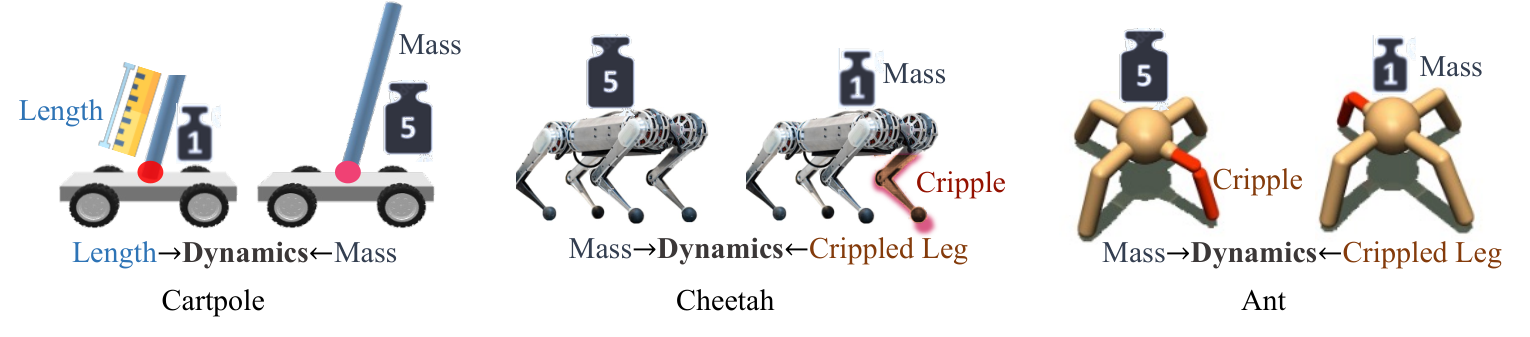

 ), length of leg (
 ), or a crippled leg (
 ). In real-world situations, all the possible confounders may change simultaneously, which bring challenges to robotic dynamics generalization.
DOMINO addresses such problem by decomposed MI optimization and achieves the state-of-the-art performance.
). In real-world situations, all the possible confounders may change simultaneously, which bring challenges to robotic dynamics generalization.
DOMINO addresses such problem by decomposed MI optimization and achieves the state-of-the-art performance.
Contribution. In this paper, we give a theoretical analysis which demonstrates that when the number of confounders increases, InfoNCE will be a loose bound of mutual information (MI) with the samples in limited seen environments, which is called MI underestimation [17]. To tackle this problem, we propose a DecOmposed Mutual INformation Optimization (DOMINO) framework for context learning in meta-RL. The context encoder aims to embed the past state-action pairs into disentangled context vectors and is optimized by maximizing the mutual information between the disentangled context vectors and historical trajectories while minimizing the state transition prediction error. DOMINO decomposes the full MI optimization problem into a summation of smaller MI optimization problems by learning disentangled context. We then theoretically prove that DOMINO could alleviate the underestimation bias of the InfoNCE and reduce the demand for the samples collected in various environments [18, 19]. Last, with the learned disentangled context, we further develop the context-aware model-based and model-free algorithms to learn the context-conditioned policy and illustrate that DOMINO can consistently improve generalization performance in both ways to overcome the challenge of multi-confounded dynamics.
Extensive experiments demonstrate that DOMINO benefits meta-RL on both the generalization performance in unseen environments and sample efficiency during the training process under the challenging multi-confounded setting. For example, as show in Figure 1(b), it achieves 1.5 times performance improvement to T-MCL [3] in the Cheetah domain and 2.6 times performance improvement to T-MCL in the Crippled-Ant domain. Visualization of the learned context demonstrates that the disentangled context generated by DOMINO under different environments could be more clearly distinguished in the embedding space, which indicates its advantage to extract high-quality contextual information from the environment.
2 Related Work
2.1 Meta-Reinforcement Learning
Meta-RL extends the framework of meta-learning [20, 21] to reinforcement learning, aiming to learn an adaptive policy being able to generalize to unseen tasks. Specifically, meta-RL methods learn the policy based on the prior knowledge discovered from various training environments and reuse the policy to fast adapt to unseen testing environments after zero or few shots. Gradient-based meta-RL algorithms [22, 23, 24, 25] learn a model initialization and adapt the parameters with few policy gradient updates in new dynamics. Context-based meta-RL algorithms [1, 2, 3, 4] learn contextual information to capture local dynamics explicitly and show great potential to tackle generalization tasks in complicated environments. Many model-free context-based methods are proposed to learn a policy conditioned on the latent context that can adapt with off-policy data by leveraging context information and is trained by maximizing the expected return. PEARL [1] adapts to a new environment by inferring latent context variables from a small number of trajectories. Recent advanced methods further improve the quality of contextual representation leveraging contrastive learning [5, 6, 7, 8]. Unlike the model-free methods mentioned above, context-aware world models are proposed to learn the dynamics with confounders directly. CaDM [26] learns a global model that generalizes across tasks by training a latent context to capture the local dynamics. T-MCL [4] combines multiple-choice learning with context-aware world model and achieves state-of-the-art results on the dynamics generalization tasks. RIA [16] further expands this method into unsupervised setting without environment label by intervention, and enhances the context learning via MI optimization.
However, existing context-based approaches focus on learning entangled context, in which each trajectory is encoded into only one context vector. In a multi-confounding environment, learning entangled contexts requires orders of magnitude higher samples to capture accurate dynamics information. To tackle this challenge, different from RIA [16] and T-MCL [4] , DOMINO infers several disentangled context vectors from a single trajectory and divides the whole MI optimization into the summation of smaller ones. The proposed decomposed MI optimization reduces the amount of demand for diverse samples and thus improves the generalization of the policy to overcome the adaptation problem in multi-confounded unseen environments.
2.2 Mutual Information Optimization for Representation Learning
Representation learning based on mutual information (MI) maximization has been applied in various tasks such as computer vision [27, 28], natural language processing [29, 19], and RL [30], exploiting noise-contrastive estimation (NCE) [31], InfoNCE [9] and variational objectives [32]. InfoNCE has gained recent interest with respect to variational approaches due to its lower variance [33] and superior performance in downstream tasks. However, InfoNCE may underestimate the true MI, given that it is limited by the number of samples. To tackle this problem, DEMI [17] first scaffolds the total MI estimation into a sequence of smaller estimation problems. In this paper, since the confounders in the real world are commonly independent, we simplify the complexity of mutual information decomposition and eliminate the need to learn conditional mutual information as a sub-term, assuming that multiple confounders are independent of each other.
3 Preliminaries
We consider standard RL framework where an agent optimizes a specified reward function through interacting with an environment. Formally, we formulate our problem as a Markov decision process (MDP) [34], which is defined as a tuple . Here, is the state space, is the action space, is the transition dynamics, is the reward function, is the initial state distribution, and is the discount factor. In order to address the problem of generalization, we further consider the distribution of MDPs, where the transition dynamics varies according to multiple confounders . The confounders can be continuous random variables, like the mass, damping, random disturbance force, or discrete random variables, such as one of the robot’s leg is crippled. We assume that the true transition dynamics model is unknown, but the state transition data can be sampled by taking actions in the environment. Given a set of training setting sampled from , the meta-training process learns a policy that adapts to the task at hand by conditioning on the embedding of the history of past transitions, which we refer as context . At test-time, the policy should adapt to the new MDP under the test setting drawn from .
Our goal is to learn a policy to maximizing the expected return condition on the context which is encoded from the sequences of current state action pairs in several training scenarios and enable it to perform well and achieve a high expected return in test scenarios never seen before.
| (1) |

 ). The context encoder embeds the past state-action pairs (
 ) into disentangled context vectors. The disentangled context vectors (
 ) are learned via the decomposed mutual information optimization (
 ) while minimizing the state transition prediction error (
 ).
Minimize transition prediction error: With the current state-action pair and the learned context vectors, future state can be predicted by the prediction network. The gradient of the prediction error will be used to update both the context encoder and the prediction network.
Decomposed MI Optimization: we optimize the MI between the learned context and the historical trajectories under the same confounder setting via maximizing the InfoNCE bound, which aims to minimize the embedding distance between the positive sampled trajectories (
).
Minimize transition prediction error: With the current state-action pair and the learned context vectors, future state can be predicted by the prediction network. The gradient of the prediction error will be used to update both the context encoder and the prediction network.
Decomposed MI Optimization: we optimize the MI between the learned context and the historical trajectories under the same confounder setting via maximizing the InfoNCE bound, which aims to minimize the embedding distance between the positive sampled trajectories ( ) and the context, while maximizing the embedding distance between the negative sampled trajectories (
 ) and the context.
4 Decomposed Mutual Information Optimization for Context Learning
In this section, we first provide a theoretical analysis to show why the multi-confounded environments are more challenging. We find that when the number of confounders increases, the InfoNCE will be a loose bound of MI with the samples in limited seen environments, resulting in the underestimation of MI. To solve such a problem, we develop the DOMINO framework to learn disentangled context by decomposed MI optimization. We theoretically illustrate that the decomposed MI optimization can alleviate the underestimation of MI and reduce the demand for the number of samples. The disentangled context is embedded by the context encoder with parameter from the past state-action pairs in current episode. DOMINO explicitly maximizes the MI between the context and the historical trajectories () collected based on the combination of multiple confounders as same as the current confounder setting, while minimizing the state transition prediction error conditioned on the learned context. We solve the MI optimization problem by optimizing the InfoNCE lower bound on MI [9], which can be viewed as a contrastive method for the MI optimization, and decompose the full MI optimization into smaller ones to alleviate the underestimation of the mutual information and reduce the demand for the number of samples collected in various environments.
4.1 InfoNCE Bound for Mutual Information Optimization
InfoNCE bound is a lower bound of the mutual information , where NCE stands for Noise-Contrastive Estimation, is a type of contrastive loss function used for self-supervised learning. InfoNCE is obtained by comparing pairs sampled from the joint distribution ( is called the positive example) to pairs built using a set of negative examples, :
| (2) |
where is a function assigning a similarity score to pairs and denotes the number of samples. Through discriminating naturally the paired positive instances from the randomly paired negative instances, it is proved to bring universal performance gains in various domains, such as computer vision and natural language processing.
Lemma 1
is a necessary condition for to be a tight bound of . (see proof in Appendix A)
Some previous context-aware methods learn an entangled context by maximizing the mutual information between the context embedded from the past state-action pairs in the current episode, and the historical trajectories collected under the same confounder setting as the current episode. They solve this problem by maximizing the InfoNCE lower bound on , which can be viewed as a contrastive estimation [9] of , and obtain promising improvement in single-confounded environment. However, according to Lemma 1, the may be loose if the true mutual information is larger than , which is called underestimation of the mutual information. Therefore, to make the InfoNCE bound to be a tight bound of , the minimum number of samples is . In real-world robotic control tasks, the dynamics of the robot is commonly influenced by multiple confounders simultaneously, under the assumption that the confounders are independent (such as mass and damping), the mutual information between the historical trajectories and the context can be derived as
| (3) |
As the number of confounders increases, the lower bound of will become larger, and the necessary condition for to be a tight bound of will become more difficult to satisfy. Since , to let the necessary consition satisfied, the amount of data must be larger than according to Lemma 1. Thus the demand for data increases significantly. Since the confounders are commonly independent in real-world, can we relax this condition by learning disentangled context vectors instead of entangled context intuitively?
4.2 Decomposed MI Optimization
If the context vectors can be independent, then we can ease this problem by applying the chain rule on MI to decompose the total MI into a sum of smaller MI terms, i.e.,
| (4) |
Theorem 1
If the context vectors can be independent, then the necessary condition for to be a tight bound can be relaxed to . Thus, the need of the number of samples can be reduced from to .
Inspired by Theorem 1, we intuitively learn disentangled context vectors and maximize the mutual information between the historical trajectories and the context vectors while minimizing the between the context vectors, i.e., to maximize the
| (5) |
where the can be obtained with the positive trajectory and negative trajectories , i.e.,
| (6) |
The context () is encoded from the past state action pairs in current episode by . Both the positive trajectory (collected in same setting of the confounders) and negative trajectory (collected in different setting of the confounders) are encoded to by . The critic function measures the cosine similarity between inputs by dot product after normalization. Under the assumption that the setting of confounders will not change in one episode, to obtain the , we use sampled from same episode like as the positive example, and use sampled from different episode as the negative example. Thus the can be derived as
| (7) |
Then, the future state can be predicted with the the current state , action and the disentangled context vectors by the state transition prediction network . We aim to minimize the prediction loss, which is equal to maximizing
| (8) |
where is the training set, and is the prediction horizon. The whole framework of DOMINO is demonstrated in Figure 2 and the overall objective function of DOMINO is
| (9) |
4.3 Combine DOMINO with Downstream RL Methods
Combination with Model-based RL. With DOMINO we can learn the context encoder and the context-aware world model together. First, the past state-action pairs are encoded into the disentangled context vectors by the context encoder. According to the learned context, the transition prediction network predicts the future states of different actions. In particular, we use the cross entropy method (CEM) [35], a typical neural model predictive control (MPC) [36] method, to select actions, in which several candidate action sequences are iteratively sampled from a candidate distribution, which is adjusted based on best-performing action samples. The optimal action sequence can be obtained by
| (10) |
Then, we use the mean value of adjusted candidate distribution as action and re-plan at every timestep. We provide detailed algorithm pseudo-code in the Appendix B.1. As for the adaptation process, the policy and context encoder zero-shot adapts to the unseen confounders setting , and we use the same adaptive planning method as T-CML[3], which selects the most accurate prediction head over a recent experience condition on the inferred context. The details is introduced in Appendix D.4
Combination with Model-free RL. Previous works show that a policy learned by model-free method can be more robust to dynamics changes when it takes the contextual information as an additional input [37, 38, 39]. Motivated by this, we investigate whether the context encoder learned by DOMINO can be used as a plug-and-play module to improve the final generalization performance of model-free RL methods. We concatenate the disentangled context encoded by a pre-trained context encoder from DOMINO and the current state-action pairs, and learn a conditional policy . We use the Proximal Policy Optimization (PPO) method to train the agent [40], which learns the policy by maximizing
| (11) |
where is the estimation of the advantage function at timestep . We provide detailed pseudo-code in the Appendix B.2.
5 Experiments
In this section, we evaluate the performance of our DOMINO method to answer the following questions: (1) Can DOMINO help the model-based RL methods overcome the multi-confounded challenges in dynamics generalization (see comparison with ablation in Figure 3 and Figure 5)? (2) Can the context encoder learned by DOMINO be used as a plug-and-play module to improve the generalization abilities of model-free RL methods in multi-confounded environments (see comparison with ablation in Table 1 and Table 3)? (3) Can the proposed decomposed MI optimization benefit the forward prediction of the world model? (see Figure 3) (4) Does the disentangled context extract more meaningful contextual information than entangled context (see Figure 7)?
5.1 Setups
We demonstrate the effectiveness of our proposed method on 8 benchmarks, which contain 6 typical robotic control tasks based on the MuJoCo physics engine [41] and 2 classical control tasks (CartPole and Pendulum) from OpenAI Gym [42]. Different from previous works, all the environments are influenced by multiple confounders simultaneously. In our experiments, we modify multiple environment parameters at the same time (e.g., mass, length, damping, push force, and crippled leg) that characterize the transition dynamics. The robotic control tasks contain 4 environments (Hopper, HalfCheetah, Ant, SlimHumanoid) affected by multiple continuous confounders and 2 more difficult environments (Crippled Ant and Crippled HalfCheetah) affected by both continuous and discrete confounders. The detailed settings are illustrated in Appendix C (Table 3). We implement these environments based on the publicly available code provide by [43, 4], and we also open-source the code of the multiple-confounded environments11 1 https://anonymous.4open.science/r/Multiple-confounded-Mujoco-Envs-01F3. For both training and testing phase, we sample the confounders at the beginning of each episode. During training, we randomly select a combination of confounders from a training set. At test time, we evaluate each algorithm in unseen environments with confounders outside the training range.
5.2 Comparison with Model-based Methods
Baselines. We consider T-MCL [3] and RIA[16] as the key baselines in comparison with model-based methods, which achieve the state-of-the-art results in zero-shot dynamics generalization tasks. Since RIA doesn’t has a adaptive planning process, we provide the DOMINO and T-MCL without adaptive planning to fair compare to the RIA. We also consider an ablation version of DOMINO as a baseline (denoted as MINO) to show the effectiveness of the decomposed MI optimization, which optimizes the MI and predicts the future states with an entangled context without decomposition.
Results. As shown in Figure 9, DOMINO achieves better generalization performance than RIA and TMCL even without the adaptive planning, especially in complex environments like Halfcheetah-- and Slim-humanoid--. Figure 3 shows the average return during the learning process in the training environments. The results illustrate that DOMINO learns the policy more efficiently than T-MCL and MINO.

Figure 5 shows the generalization performance tested in the unseen environments. The results show that DOMINO surpasses T-MCL in terms of the generalization performance and the learning sample efficiency. This demonstrates that the disentangled context improves the context-aware world model. Especially, the performance gain becomes much more significant in more complex environments (e.g., long-horizon and high-dimensional domains like Cripple-Ant, Ant, and Hopper). For example, DOMINO achieves about 2.6 times improvement to T-MCL in Cripple-Ant--, which is one of the most difficult environment, whose leg will randomly be crippled, and its mass and damping will be changed in testing. More details are shown in Appendix D.
5.3 Comparison with Model-free Methods
We also verify whether the learned disentangled context is useful for improving the generalization performance of model-free RL methods. Similar to [3, 44], we use the Proximal Policy Optimization (PPO [40]) method to train the agents.
Baselines. Our proposed method, which takes the context learned by DOMINO as conditional input (PPO+DOMINO), is compared with several context-conditional policies [45, 39]. Specifically, we consider combining the PPO with the context learned by T-MCL (PPO+T-MCL), which learns the context encoder via a context-aware world model and achieves the state-of-the-art performance on dynamics generalization. We also consider PEARL [45], which learns probabilistic context variable by maximizing the expected returns. We further develop an ablation version of DOMINO, which optimize the MI with entangled context (PPO+MINO) as a baseline to illustrate the effectiveness of the decomposed MI optimization. We provide more detailed explanations in Appendix D.
Results. Table 1 and Table 3 show the performance of various model-free RL methods on both training and test environments. PPO+DOMINO shows superior performance and shows better generalization performances than previous conditional policy methods, implying that the proposed DOMINO method can extract contextual information more effectively than both the context learned by the model-based method (PPO+T-MCL) and the context learned by the model-free method (PEARL). Furthermore, PPO+DOMINO shows an obvious advantage over PPO+MINO, especially in complex environments, such as HalfCheetah, Ant, and Hopper, which implies that the decomposed MI optimization improves the context learning significantly. Additionally, the results also show that compared to PEARL, the context learned by T-MCL and DOMINO has better performance which implies that the state transition perdition can help to extract contextual information more effectively.
Cartpole-- Pendulum-- Ant-- Train Test Train Test Train Test PEARL 197 175 -1265 -1293 153 73 PPO+T-MCL 220 182 -558 -579 176 173 PPO+MINO 267 234 -497 -526 194 PPO+DOMINO 299 283 -405 -436 227 216 Halfcheetah-- Slimhumanoid-- Hopper-- Train Test Train Test Train Test PEARL 1802 530 6947 3697 934 874 PPO+T-MCL 2032 674 6157 4136 937 896 PPO+MINO 1973 824 6179 4275 1109 964 PPO+DOMINO 2472 1034 7825 5258 1409 1137
Cripple-Ant-- Cripple-Halfcheetah-- Train Test Train Test PEARL 182 96 2538 1028 PPO+T-MCL 187 109 2368 1006 PPO+MINO 206 113 2493 1197 PPO+DOMINO 233 132 2503 1326
5.4 Disentangled Context Analysis
Prediction errors. To show that our method indeed helps with a transition prediction, we compare baseline methods with DOMINO in terms of prediction error across 8 environments with varying multiple confounders. As shown in Figure 3, our model demonstrates superior prediction performance, which indicates that the learned context capture better contextual information compare with entangled context (see more results in Appendix E.1).
Visualization. We visualize concatenation of the disentangled context vectors learned by DOMINO via t-SNE [46] and compare it with the entangled context learned by T-MCL. As shown in Figure 7, we find that the disentangled context vectors encoded from trajectories collected under different confounder settings could be more clearly distinguished in the embedding space than the entangled context learned by T-MCL. This indicates that DOMINO extracts high-quality task-specific information from the environment compared with T-MCL. We provide more visualization results based on both t-SNE [46] and PCA [47] in Appendix F.2.
6 Conclusion
In this paper, we propose a decomposed mutual information optimization (DOMINO) framework to learn the generalized context for zero-shot dynamics generalization. The disentangled context is learned by maximizing the mutual information between the context and historical trajectories while minimizing the state transition prediction error. By decomposing the whole mutual information optimization problem into smaller ones, DOMINO can reduce the need for samples collected in various environments and overcome the underestimation of the mutual information in multi-confounded environments. Extensive experiments illustrate that DOMINO benefits the generalization performance in unseen environments with both model-based RL and model-free RL. For future work, an effective combination of DOMINO and RIA [16], which expands the decomposed MI optimization to relational intervention approach proposed by RIA could become a stronger baseline for unsupervised dynamics generalization. We believe our work can lay the foundation of dynamics generalization in complex environments.
Limitations and Negative Social Impact. DOMINO sets the number of disentangled context vectors as a hyper-parameter equal to the number of confounders in the environments, and capturing the number of confounders automatically could be future works. We believe that DOMINO will not cause any negative social impact.
Acknowledgments and Disclosure of Funding
The authors would like to thank the anonymous reviewers for their valuable comments and helpful suggestions. The work is supported by Huawei Noah’s Ark Lab; Ping Luo is supported by the General Research Fund of HK No.27208720, No.17212120, and No.17200622.
References
- [1] Kate Rakelly, Aurick Zhou, Chelsea Finn, Sergey Levine, and Deirdre Quillen. Efficient off-policy meta-reinforcement learning via probabilistic context variables. In Proceedings of the 36th International Conference on Machine Learning, ICML 2019, pages 5331–5340, 2019.
- [2] Rasool Fakoor, Pratik Chaudhari, Stefano Soatto, and Alexander J. Smola. Meta-q-learning. In 8th International Conference on Learning Representations, ICLR 2020. OpenReview.net, 2020.
- [3] Kimin Lee, Younggyo Seo, Seunghyun Lee, Honglak Lee, and Jinwoo Shin. Context-aware dynamics model for generalization in model-based reinforcement learning. In International Conference on Machine Learning, 2020.
- [4] Younggyo Seo, Kimin Lee, Ignasi Clavera, Thanard Kurutach, Jinwoo Shin, and Pieter Abbeel. Trajectory-wise multiple choice learning for dynamics generalization in reinforcement learning. arXiv preprint arXiv:2010.13303, 2020.
- [5] Haotian Fu, Hongyao Tang, Jianye Hao, Chen Chen, Xidong Feng, Dong Li, and Wulong Liu. Towards effective context for meta-reinforcement learning: an approach based on contrastive learning. arXiv preprint arXiv:2009.13891, 2020.
- [6] Bernie Wang, Simon Xu, Kurt Keutzer, Yang Gao, and Bichen Wu. Improving context-based meta-reinforcement learning with self-supervised trajectory contrastive learning. arXiv preprint arXiv:2103.06386, 2021.
- [7] Lanqing Li, Yuanhao Huang, Mingzhe Chen, Siteng Luo, Dijun Luo, and Junzhou Huang. Provably improved context-based offline meta-rl with attention and contrastive learning. arXiv preprint arXiv:2102.10774, 2021.
- [8] Tong Sang, Hongyao Tang, Yi Ma, Jianye Hao, Yan Zheng, Zhaopeng Meng, Boyan Li, and Zhen Wang. Pandr: Fast adaptation to new environments from offline experiences via decoupling policy and environment representations. arXiv preprint arXiv:2204.02877, 2022.
- [9] Aaron van den Oord, Yazhe Li, and Oriol Vinyals. Representation learning with contrastive predictive coding. arXiv preprint arXiv:1807.03748, 2018.
- [10] Michael Dennis, Natasha Jaques, Eugene Vinitsky, Alexandre Bayen, Stuart Russell, Andrew Critch, and Sergey Levine. Emergent complexity and zero-shot transfer via unsupervised environment design. Advances in neural information processing systems, 33:13049–13061, 2020.
- [11] Minqi Jiang, Edward Grefenstette, and Tim Rocktäschel. Prioritized level replay. In International Conference on Machine Learning, pages 4940–4950. PMLR, 2021.
- [12] Minqi Jiang, Michael Dennis, Jack Parker-Holder, Jakob Foerster, Edward Grefenstette, and Tim Rocktäschel. Replay-guided adversarial environment design. Advances in Neural Information Processing Systems, 34:1884–1897, 2021.
- [13] Jack Parker-Holder, Minqi Jiang, Michael Dennis, Mikayel Samvelyan, Jakob Foerster, Edward Grefenstette, and Tim Rocktäschel. Evolving curricula with regret-based environment design. arXiv preprint arXiv:2203.01302, 2022.
- [14] Roberta Raileanu and Rob Fergus. Decoupling value and policy for generalization in reinforcement learning. In International Conference on Machine Learning, pages 8787–8798. PMLR, 2021.
- [15] Karl Cobbe, Christopher Hesse, Jacob Hilton, and John Schulman. Leveraging procedural generation to benchmark reinforcement learning, arxiv. arXiv preprint arXiv:1912.01588, 2019.
- [16] Jiaxian Guo, Mingming Gong, and Dacheng Tao. A relational intervention approach for unsupervised dynamics generalization in model-based reinforcement learning. In International Conference on Learning Representations, 2022.
- [17] Alessandro Sordoni, Nouha Dziri, Hannes Schulz, Geoff Gordon, Philip Bachman, and Remi Tachet Des Combes. Decomposed mutual information estimation for contrastive representation learning. In International Conference on Machine Learning, pages 9859–9869. PMLR, 2021.
- [18] David McAllester and Karl Stratos. Formal limitations on the measurement of mutual information. In International Conference on Artificial Intelligence and Statistics, pages 875–884. PMLR, 2020.
- [19] Karl Stratos. Mutual information maximization for simple and accurate part-of-speech induction. arXiv preprint arXiv:1804.07849, 2018.
- [20] Juergen Schmidhuber. Evolutionary principles in self-referential learning. 1987.
- [21] Sebastian Thrun and Lorien Y. Pratt. Learning to learn. In Springer US, 1998.
- [22] Chelsea Finn, Pieter Abbeel, and Sergey Levine. Model-agnostic meta-learning for fast adaptation of deep networks. In Proceedings of the 34th International Conference on Machine Learning, ICML 2017, pages 1126–1135, 2017.
- [23] Jonas Rothfuss, Dennis Lee, Ignasi Clavera, Tamim Asfour, and Pieter Abbeel. Promp: Proximal meta-policy search. In 7th International Conference on Learning Representations, ICLR 2019, 2019.
- [24] H. Liu, R. Socher, and Caiming Xiong. Taming maml: Efficient unbiased meta-reinforcement learning. In ICML, 2019.
- [25] A. Gupta, R. Mendonca, Yuxuan Liu, P. Abbeel, and S. Levine. Meta-reinforcement learning of structured exploration strategies. In NeurIPS, 2018.
- [26] Kimin Lee, Younggyo Seo, Seunghyun Lee, Honglak Lee, and Jinwoo Shin. Context-aware dynamics model for generalization in model-based reinforcement learning. CoRR, abs/2005.06800, 2020.
- [27] Jean-Bastien Grill, Florian Strub, Florent Altché, Corentin Tallec, Pierre H Richemond, Elena Buchatskaya, Carl Doersch, Bernardo Avila Pires, Zhaohan Daniel Guo, Mohammad Gheshlaghi Azar, et al. Bootstrap your own latent: A new approach to self-supervised learning. arXiv preprint arXiv:2006.07733, 2020.
- [28] Mathilde Caron, Ishan Misra, Julien Mairal, Priya Goyal, Piotr Bojanowski, and Armand Joulin. Unsupervised learning of visual features by contrasting cluster assignments. arXiv preprint arXiv:2006.09882, 2020.
- [29] Tomas Mikolov, Kai Chen, Greg Corrado, and Jeffrey Dean. Efficient estimation of word representations in vector space. arXiv preprint arXiv:1301.3781, 2013.
- [30] Bogdan Mazoure, Remi Tachet des Combes, Thang Doan, Philip Bachman, and R Devon Hjelm. Deep reinforcement and infomax learning. 2020.
- [31] Michael U Gutmann and Aapo Hyvärinen. Noise-contrastive estimation of unnormalized statistical models, with applications to natural image statistics. Journal of Machine Learning Research, 13:307–361, 2012.
- [32] R Devon Hjelm, Alex Fedorov, Samuel Lavoie-Marchildon, Karan Grewal, Phil Bachman, Adam Trischler, and Yoshua Bengio. Learning deep representations by mutual information estimation and maximization. 2019.
- [33] Jiaming Song and Stefano Ermon. Understanding the limitations of variational mutual information estimators. 2019.
- [34] Richard S Sutton and Andrew G Barto. Reinforcement learning: An introduction. MIT Press, 2018.
- [35] Zdravko I Botev, Dirk P Kroese, Reuven Y Rubinstein, and Pierre L’Ecuyer. The cross-entropy method for optimization. In Handbook of statistics. Elsevier, 2013.
- [36] Carlos E Garcia, David M Prett, and Manfred Morari. Model predictive control: theory and practice—a survey. Automatica, 25(3):335–348, 1989.
- [37] Wenhao Yu, Jie Tan, C Karen Liu, and Greg Turk. Preparing for the unknown: Learning a universal policy with online system identification. In RSS, 2018.
- [38] Charles Packer, Katelyn Gao, Jernej Kos, Philipp Krähenbühl, Vladlen Koltun, and Dawn Song. Assessing generalization in deep reinforcement learning. arXiv preprint arXiv:1810.12282, 2018.
- [39] Wenxuan Zhou, Lerrel Pinto, and Abhinav Gupta. Environment probing interaction policies. In ICLR, 2019.
- [40] John Schulman, Filip Wolski, Prafulla Dhariwal, Alec Radford, and Oleg Klimov. Proximal policy optimization algorithms. arXiv preprint arXiv:1707.06347, 2017.
- [41] Emanuel Todorov, Tom Erez, and Yuval Tassa. Mujoco: A physics engine for model-based control. In IROS, 2012.
- [42] Greg Brockman, Vicki Cheung, Ludwig Pettersson, Jonas Schneider, John Schulman, Jie Tang, and Wojciech Zaremba. Openai gym. arXiv preprint arXiv:1606.01540, 2016.
- [43] Anusha Nagabandi, Ignasi Clavera, Simin Liu, Ronald S Fearing, Pieter Abbeel, Sergey Levine, and Chelsea Finn. Learning to adapt in dynamic, real-world environments through meta-reinforcement learning. In ICLR, 2019.
- [44] Peter Henderson, Riashat Islam, Philip Bachman, Joelle Pineau, Doina Precup, and David Meger. Deep reinforcement learning that matters. In AAAI, 2018.
- [45] Kate Rakelly, Aurick Zhou, Deirdre Quillen, Chelsea Finn, and Sergey Levine. Efficient off-policy meta-reinforcement learning via probabilistic context variables. In ICML, 2019.
- [46] Laurens van der Maaten and Geoffrey Hinton. Visualizing data using t-sne. Journal of Machine Learning Research, 9(Nov):2579–2605, 2008.
- [47] Ian T Jolliffe. Principal component analysis for special types of data. Springer, 2002.
- [48] David Barber and Felix Agakov. The im algorithm: A variational approach to information maximization. page 201–208, 2003.
- [49] Chris Cremer, Quaid Morris, and David Duvenaud. Reinterpreting importance-weighted autoencoders. 2017.
- [50] Diederik P Kingma and Jimmy Ba. Adam: A method for stochastic optimization. In ICLR, 2015.
- [51] John Schulman, Philipp Moritz, Sergey Levine, Michael Jordan, and Pieter Abbeel. High-dimensional continuous control using generalized advantage estimation. In ICLR, 2016.
- [52] Luisa Zintgraf, Kyriacos Shiarlis, Maximilian Igl, Sebastian Schulze, Yarin Gal, Katja Hofmann, and Shimon Whiteson. Varibad: A very good method for bayes-adaptive deep rl via meta-learning. arXiv preprint arXiv:1910.08348, 2019.
Checklist
- 1.
For all authors…
- (a)
Do the main claims made in the abstract and introduction accurately reflect the paper’s contributions and scope? [Yes]
- (b)
Did you describe the limitations of your work? [Yes]
- (c)
Did you discuss any potential negative societal impacts of your work? [Yes]
- (d)
Have you read the ethics review guidelines and ensured that your paper conforms to them? [Yes]
- (a)
- 2.
- 3.
If you ran experiments…
- (a)
- (b)
Did you specify all the training details (e.g., data splits, hyperparameters, how they were chosen)? [Yes] See Appendix D.
- (c)
Did you report error bars (e.g., with respect to the random seed after running experiments multiple times)? [Yes] See Section 5.
- (d)
Did you include the total amount of compute and the type of resources used (e.g., type of GPUs, internal cluster, or cloud provider)? [Yes] See Appendix D.
- 4.
If you are using existing assets (e.g., code, data, models) or curating/releasing new assets…
- (a)
If your work uses existing assets, did you cite the creators? [Yes]
- (b)
Did you mention the license of the assets? [N/A]
- (c)
Did you include any new assets either in the supplemental material or as a URL? [Yes]
- (d)
Did you discuss whether and how consent was obtained from people whose data you’re using/curating? [N/A]
- (e)
Did you discuss whether the data you are using/curating contains personally identifiable information or offensive content? [N/A]
- (a)
- 5.
If you used crowdsourcing or conducted research with human subjects…
- (a)
Did you include the full text of instructions given to participants and screenshots, if applicable? [N/A]
- (b)
Did you describe any potential participant risks, with links to Institutional Review Board (IRB) approvals, if applicable? [N/A]
- (c)
Did you include the estimated hourly wage paid to participants and the total amount spent on participant compensation? [N/A]
- (a)
Appendix A Derivations
A.1 Proof of Lemma 1
According to the Barber and Agakov’s variational lower bound [48], the mutual information between and can be bounded as follows:
| (12) |
where is an arbitrary distribution. Specifically, is defined by independently sampling a set of examples from a proposal distribution and then choosing from in proportion to the importance weights , where is a function that takes and and outputs a scalar. According to the section 2.3 in [9], by setting the proposal distribution as the marginal distribution , the unnormalized density of given a specific set of samples and is:
| (13) |
where denotes the numbers of samples. According to the equation 3 of section 2 in [49], the expectation of with respect to resampling of the alternatives from produces a normalized density:
| (14) |
With Equation 14 and Jensen’s inequality applied in Equation 12, we have
| (15) | ||||
It is obviously that , thus we have
| (16) |
With Equation 16, we have
| (17) | ||||
Therefore, we have
| (18) |
If , then , and will be a loose bound.
Thus, is the necessary condition for to be a tight bound of .
A.2 Detailed derivation of Theorem 1
As the number of confounders increases, although the true mutual information does not increase, the necessary condition of to be a tight lower bound of becomes more difficult to satisfy, and the demand of data increases significantly.
As for an entangled context, the necessary condition of the InfoNCE lower bound to be a tight bound is
| (19) |
Since , to let the above condition satisfied, the amount of data must satisfy
| (20) |
| (21) |
Therefore, if the number of confounders increases, then the demand for data will grow exponentially.
When data is not rich enough, the nesseray condition may not be satisfied. The InfoNCE lower bound may be loose, that is may be much smaller than the true mutual information , thus the MI optimization based on will be severely affected.
is the lower bound of and the necessary condition of to be a tight bound of is
| (22) |
As for disentangled context , we then derive the necessary condition of to be a tight lower bound of :
With the assumption that the contexts are independent to each other, then could be derived as . Therefore, under the confounder independent assumption, let be a tight bound is only necessary to let every to be a tight bound.
If every is a tight bound, then we have
| (23) |
under the confounder independent assumption, we have
| (24) |
| (25) |
Thus, the necessary condition of to be a tight bound of could be relaxed to
| (26) |
Therefore, by decomposing the MI estimation under the confounder independent assumption, the demand of the amount of data could be reduced from to . And with , specificly, the the amount of data could be reduced from to .
Appendix B Pseudo-code
B.1 Combination with model-based methods
We provide the pseudo-code of DOMINO combined with model-based methods. Firstly, the past state-action pairs are encoded into the disentangled context vectors by the context encoder. According to the learned context, the transition prediction network predicts the future states of different actions. Then, the context encoder is optimized by maximizing the mutual information between the disentangled context vectors and historical trajectories while minimizing the state transition prediction error. In particular, we use the cross entropy method (CEM) [35], a typical neural model predictive control (MPC) [36] method, to select actions, in which several candidate action sequences are iteratively sampled from a candidate distribution, which is adjusted based on best-performing action samples.
B.2 Combination with model-free methods
We provide the pseudo-code for the combination between DOMINO and the model-free method, which uses the context encoder learned by DOMINO as a plug-and-play module to extract accurate context. We concatenate the disentangled context encoded by a pre-trained context encoder from DOMINO and the current state-action pairs, and learn a conditional policy . We choose the Proximal Policy Optimization (PPO) method [40] to train the agents.
Appendix C Details about the testing environments
Train Test CartPole Pendulum Half-cheetah Ant SlimHumanoid Crippled Ant crippled leg: crippled leg: Crippled Halfcheetah crippled leg: crippled leg:
For CartPole environments, we use open-source implementation of CartPoleSwingUp-v222 2 We use implementation available at https://github.com/0xangelo/gym-cartpole-swingup, which is the modified version of original CartPole environments from OpenAI Gym. The objective of CartPole task is to swing up the pole by moving a cart and keep the pole upright. For our experiments, we modify the push force and the pole length simultaneously. As for Pendulum, we scale the pendulum mass by scale factor and modify the pendulum length . For Pendulum environments, we use the open-source implementation of from the OpenAI Gym. The objective of Pendulum is to swing up the pole and keep the pole upright within 200 timesteps. We scale the pendulum mass by scale factor and modify the pendulum length .
As for Hopper, Half-cheetah, Ant, and Slimhumanoid, we use the environments from MuJoCo physics engine 33 3 We use implementation available at https://github.com/iclavera/learning_to_adapt, and scale the mass of every rigid link by scale factor , and scale damping of every joint by scale factor . As for Crippled Ant and Crippled Half-cheetah, we scale the mass of every rigid link by scale factor , scale damping of every joint by scale factor , and randomly select one leg, and make it crippled. The objectives of these tasks are to move forward as fast as possible while minimizing the action cost. The detailed settings are illustrated in Table 3. We provide the pyTorch-style pseudo-code for multi-confounded environments in Listing 1 and Listing 2. We implement these environments based on the publicly available code provide by [43, 4], and we also open-source the code of the multiple-confounded environments44 4 We provide open-source environments at https://anonymous.4open.science/r/Multiple-confounded-Mujoco-Envs-01F3. For both the training and testing phase, we sample the confounders at the beginning of each episode. During training, we randomly select a combination of confounders from a training set. At test time, we evaluate each algorithm in unseen environments with confounders outside the training range. We also provide the PyTorch-style pseudo-code for the dynamics change based on Mujoco engine.
Appendix D Implementation details
D.1 Combination with Model-based RL
The context encoder is modeled as multi-layer perceptrons (MLPs) with 3 hidden layers and N output heads which are single-layer MLPs. Every disentangled context vector is produced as a 10-dimensional vector by the 3 hidden layers and a specific output head. Then, the disentangled context vectors are used as the additional input to the prediction network, i.e., the input is given as a concatenation of state, action, and context vector. We use for the number of past observations and for the number of future observations. The prediction network is modeled as multi-layer perceptrons (MLPs) with 4 hidden layers of 200 units each and Swish activations. For each prediction head, the mean and variance are parameterized by a single linear layer that takes the output vector of the backbone network as an input. To train the prediction network, we collect 10 trajectories with 200 timesteps from environments using the MPC controller and train the model for 50 epochs at every iteration. We train the prediction network for 10 iterations for every experiment. We evaluate trained models on environments over 8 random seeds every iteration to report the testing performance. The Adam optimizer [50] is used with a learning rate . For planning, we use the cross entropy method (CEM) with 200 candidate actions for all the environments. The horizon of MPC is set as 30.
D.2 Combination with Model-free RL
We train the model-free agents for 5 million timesteps on OpenAI-Gym and MuJoCo environments (i.e., Hopper, Half-cheetah, Ant, Crippled Half-cheetah, Crippled Half-Ant, Slim-Humanoid) and 0.5 million timesteps on CartPole and Pendulum. The trained agents are evaluated every 10,000 timesteps over 5 random seeds. We use a discount factor , a generalized advantage estimator [51] parameter and an entropy bonus of 0.01 for exploration. In every iteration, the agent rollouts 200 timesteps in the environments with the learned policy, and then it will be trained for 8 epochs with 4 mini-batches. The Adam optimizer is used with the learning rate .
D.3 Details of InfoNCE
We provide detailed pseudocode for the calculation of InfoNCE bound. Specifically, the temperature is set as 0.004 to the calculation of and is set as 0.1 to calculation of .
D.4 Details of the adaptive planning used in adaption process
The prediction model has 3 output head which are used for selecting actions by planning. The adaptive planning method selects the most accurate prediction head over a recent experience. Given past transitions, we select the prediction head by
where is the mean square error function. All the hyper-parameter is set as same as T-MCL[3].
Appendix E Additional Results
E.1 Prediction Error
As shown in Figure 8, DOMINO has a smaller prediction error compared to T-MCL and its ablation version MINO (optimize MI with entangled context), indicating that the learned context can effectively help predict the future state more accurately, which is the key to the performance of the model-based planning.

E.2 More results on the comparison with RIA
We provide the comparison between the DOMINO without adaptive planning and RIA in the main paper. Here, we compare DOMINO and T-MCL with adaptive planning with RIA under multi-confounded setting, the environments including Hopper--, Halfcheetah--, Slim-humanoid-- and Pendulum--. As shown in Figure 9, DOMINO also achieves better generalization performance than RIA and the TMCL with adaptive planning.
E.3 Sensitivity Analysis of the hyper-parameter N
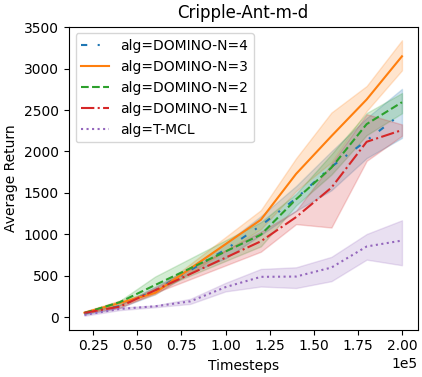
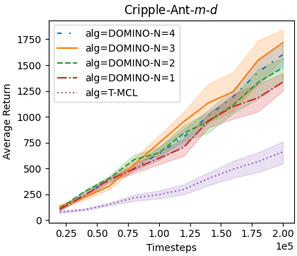
We compare the performance of DOMINO with different hyper-parameter , which is equal or not equal to the number of confounders in the environment. In this experiment, the confounder is the damping, mass, and a crippled leg (number of confounders is 3), and we compare the performance of DOMINO with different hyper-parameter . As shown in Figure 10, even though the hyper-parameter is not equal to the ground truth value of the confounder number, DOMINO also benefits the context learning compared to the baselines like TMCL.
Appendix F Visualization
F.1 Verifying whether the contexts is disentangled
We add an additional experiment to show that the context vectors inferred by DOMINO are disentangled well. We vary only one of the confounders and observe the changes of disentangled vectors. In this experiment, we set up two different confounders: mass and damping . Under the DOMINO framework, the context encoder inferred two disentangled context vectors: context 0 and context 1. As shown in Figure 12 and Figure 11, the context 1 is more related to damping. When the confounders are set as the same mass but different damping, the visualization result of context 1 under different settings are separated clearly from each other, while under the same damping but different mass settings, the visualization result of context 1 is much more blurred from each other. Similarly, context 0 is more related to mass. When the confounders are set to the same damping but different mass, the visualization result of context 0 under different settings is separated clearly from each other, while under the same mass but different damping settings, the visualization result of context 0 is less different from each other.


F.2 Visualization of the whole context
Visualization. We visualize the whole context which is a the concatenation of the disentangled contexts learned by DOMINO via t-SNE [46] and compare it with the entangled context learned by T-MCL. We run the learned policies under 5 randomly sampled setups of multiple confounders and collect 200 trajectories for each setting. Further, we encode the collected trajectories into context in embedding space and visualize via t-SNE [46] and PCA [47]. As shown in Figure 13 and Figure 14, we find that the disentangled context vectors encoded from trajectories collected under different confounder settings could be more clearly distinguished in the embedding space than the entangled context learned by T-MCL. This indicates that DOMINO extracts high-quality task-specific information from the environment compared with T-MCL. Accordingly, the policy conditioned on the disentangled context is more likely to get a higher expected return on dynamics generalization tasks, which is consistent with our prior empirical findings.

Appendix G Further discussion about the future works
G.1 Expand DOMINO into reward generalization
The reward generalization can be categorized as a kind of task generalization. The parameter of the reward function, for example, the target speed of the robot, can also be considered as a confounder that influences the reward transition. To address this problem under the DOMINO framework, we provide the following solution. The context encoder maps the current sequence of state-action-reward pairs into disentangled contexts, which contains the information of the physical confounders like mass and damping and the reward confounder. The historical trajectory also should consider the reward part, i.e., . Then the proposed decomposed mutual information optimization method can also be used in this situation to extract effective context. Moreover, the prediction loss should also add the reward prediction term. Thus, with the above design, DOMINO can address the reward generalization and dynamics generalization simultaneously.
G.2 Expand DOMINO to support related confounders
To further support the complex environment with confounders related to each other, we can explore how to extract the information that is most useful for state transfer from each of the confounders separately when they do have some correlation with each other. One possible option is to adjust the penalty factor for mutual information between the context vectors in DOMINO, which can be set to be dynamically adjustable.
G.3 Combined with VariBad and RIA
VariBad [52] introduces the VAE method and recurrent network to learn the context, which optimizes the context learning from different perspectives from DOMINO and TMCL methods. We believe the effective combination of DOMINO and Varibad will become a more powerful baseline for meta-RL. RIA[16] doesn’t need to record if the two trajectories are collected in the same episode, since the relational intervention approach could optimize the mutual information without environment labels and even without the environment ID, which provides a promising direction of unsupervised dynamics generalization. We believe that DOMINO and RIA are not in competition, on the contrary, their effective combination will become a stronger baseline, for example, the decomposed MI optimization can be expanded into the relational intervention approach proposed in RIA.