Robust analytic continuation of Green’s functions via projection, pole estimation, and semidefinite relaxation
Abstract
Green’s functions of fermions are described by matrix-valued Herglotz-Nevanlinna functions. Since analytic continuation is fundamentally an ill-posed problem, the causal space described by the matrix-valued Herglotz-Nevanlinna structure can be instrumental in improving the accuracy and in enhancing the robustness with respect to noise. We demonstrate a three-pronged procedure for robust analytic continuation called PES: (1) Projection of data to the causal space. (2) Estimation of pole locations. (3) Semidefinite relaxation within the causal space. We compare the performance of PES with the recently developed Nevanlinna and Carathéodory continuation methods and find that PES is more robust in the presence of noise and does not require the usage of extended precision arithmetics. We also demonstrate that a causal projection improves the performance of the Nevanlinna and Carathéodory methods. The PES method is generalized to bosonic response functions, for which the Nevanlinna and Carathéodory continuation methods have not yet been developed. It is particularly useful for studying spectra with sharp features, as they occur in the study of molecules and band structures in solids.
I Introduction
Green’s functions of quantum many-body systems are central subjects in condensed matter physics, quantum chemistry, and quantum field theory. Due to the difficulty of performing correlated finite-temperature calculations on the real axis, numerical methods typically obtain results on the Matsubara axis and employ analytic continuation as a postprocessing tool to infer Green’s functions along the real axis. Analytic continuation is fundamentally an ill-posed problem, and many numerical methods have been developed, such as the Padé fit Baker et al. 1996; Schött et al. 2016, maximum entropy (MaxEnt) Jarrell and Gubernatis 1996; Asakawa et al. 2001; Levy et al. 2017; Bryan 1990; Rothkopf 2020, stochastic analytic continuation and its variants Sandvik 1998; Vafayi and Gunnarsson 2007; Fuchs et al. 2010; Shao and Sandvik 2022, sparse modeling Yoshimi et al. 2019; Motoyama et al. 2022, and machine learning approaches Fournier et al. 2020; Yoon et al. 2018. All these methods encounter difficulties in satisfying causality, recovering sharp features, resolving multiple features, and/or capturing high frequency information in the spectra. Furthermore, most methods have been developed only for diagonal entries of the Green’s function. The analytic continuation of off-diagonal entries of the Green’s function Tomczak and Biermann 2007; Dang et al. 2014; Gull and Millis 2014; Kraberger et al. 2017; Reymbaut et al. 2017 is often attempted by diagonalizing the Green’s function at a certain Matsubara frequency, conducting the analytic continuation only of the diagonal entries with respect to the transformed basis at other frequencies, and neglecting the remaining non-diagonal entries.
The fermionic Green’s functions is a special type of matrix-valued Herglotz-Nevanlinna functions. These functions have a wide range of scientific and engineering applications, and have been (somewhat inconsistently) named after renowned mathematicians including Carathéodory, Herglotz, Nevanlinna, Pick, and Riesz. They are also sometimes called -functions Kac and Krein 1974. The name matrix-valued Herglotz-Nevanlinna functions adopted in this paper follows the suggestion in Belyi et al. 2006. This crucial analytic structure has only been taken into account recently by the Nevanlinna continuation method Fei et al. 2021a for diagonal entries of Green’s functions, and by the Carathéodory method Fei et al. 2021b for both diagonal and off-diagonal entries. In the absence of noise, these methods have reached unprecedented accuracy in analytic continuation by resolving complicated spectral functions with multiple features. However, these methods also have notable drawbacks. (1) They are not numerically stable, and extended precision arithmetic operations (128 bits of precision or higher) are needed to carry out such calculations (even in the absence of noise). Therefore the computational cost of the analytic continuation (especially for the Carathéodory continuation) can be large. (2) The Nevanlinna/Carathéodory interpolants exist if and only if Pick’s criterion Pick 1917; Khargonekar and Tannenbaum 1985; Fei et al. 2021a is satisfied by the Matsubara data. In practice, noisy data often violates Pick’s criterion, meaning that the computational result is not guaranteed to be causal. (3) In their standard form, matrix-valued Herglotz-Nevanlinna structure is only applicable to fermions, and hence these methods are not directly applicable to bosonic systems.
The Herglotz-Nevanlinna function and its interpolation have been thoroughly studied in areas such as the control theory (see e.g., Tannenbaum 1987 and (Doyle et al. 2013, Chapter 9.2)). The problem of analytic continuation is also intimately related to problems in signal processing, and in particular fitting with exponential functions (see e.g., Osborne and Smyth 1995; Golub and Pereyra 2003; Beylkin and Monzón 2005). One advantage of Nevanlinna and Carathéodory methods is that they require little prior knowledge of the structure of Green’s functions. With further prior knowledge of the lower and upper bound of the absolute value of the pole locations, Ying recently showed that a modified Prony’s method can be used for performing analytic continuation with noisy data with multiple features using only double precision arithmetic operations Ying 2022a; Ying 2022b.
In this article, we propose a three-pronged Projection-Estimation-Semidefinite relaxation (PES) method to perform analytic continuation within the causal space, while avoiding the aforementioned drawbacks. The meaning of the three steps are as follows: (1) Projection of the noisy data into the causal space; (2) Estimation of pole locations using the adaptive Antoulas–Anderson (AAA) algorithm Nakatsukasa et al. 2018; (3) Semidefinite relaxation (SDR) fitting of Green’s functions (diagonal and off-diagonal elements) using a bi-level optimization approach Mejuto-Zaera et al. 2020. Each step of the approach aims at resolving certain aspects of the difficulties in the analytic continuation of noisy Matsubara Green’s functions. The prior knowledge needed for the PES method is comparable to that in Nevanlinna and Carathéodory methods. We demonstrate that the PES method can robustly perform analytical continuation of noisy data using standard double precision arithmetic operations, and is applicable to both fermionic and bosonic systems. Table 1 compares the PES method with the Nevanlinna, Carathéodory, MaxEnt, and Padé method. We emphasize that each of the three steps of PES can also be useful in improving the robustness of other analytic continuation methods. For instance, the projection step can be employed as a data pre-processing step that significantly improves the robustness of the Nevanlinna and Carathéodory continuation for noisy data. The semidefinite relaxation can be combined with other continuation methods as a post-processing refinement.
| Method | Causality | Applicability | |||
|---|---|---|---|---|---|
| This work | ✓ | Double | ✓ | ✓ | |
| ✗ | Extended | ✓ | Fermion | ||
| MaxEnt | ✓ | Double | ✗ | ✓ | |
| Padé | ✗ | Extended | ✓ | ✗ |
This article is organized as follows. In Section II, we introduce the theory of the PES method. After giving a brief discussion on the setup of the analytic continuation problem in Section II.1, we explain in detail each of the three steps of the PES method: the pre-processing step using semidefinite projection in Section II.2, the pole-estimation step using AAA algorithm in Section II.3 and the SDR fitting step using SDR and bi-level optimization in Section II.4. We summarize the PES method in Section II.5. The numerical results are presented in Section III. With the Hubbard dimer example, we compare the results of our methods with the Nevanlinna, Carathéodory and MaxEnt methods, and show that the PES method is both noise-robust and efficient for sharp features, and recovers both diagonal and off-diagonal entries. We also demonstrate the necessity of the pole estimation step using this model. In Section III.2, we show that the PES method is also applicable to bosonic response functions and has a much better performance compared to MaxEnt. In Section III.3, in order to demonstrate the strength of the PES method, we conduct analytic continuations for the band structure of solids with hundreds of orbitals.
II Theory
II.1 Analytic structure of Green’s functions
Let be the annihilation and creation operator for the -th orbital, , where is the number of orbitals. In the Lehmann representation, a Green’s function can be expressed as follows (see e.g., (Negele and Orland 1988, Chapter 5.2)):
| (1) |
Here is the inverse temperature. is the -th eigenfunction of the Hamiltonian with energy , i.e.,
where , is the many-body Hamiltonian and is the partition function. The negative sign corresponds to bosons, while the positive sign corresponds to fermions.
Since is defined for , the Green’s function can be viewed as a matrix. In other words, we have where and is a rank-1 matrix, in which
| (2) |
Here is the -th component of . Note that for fermionic systems, is always nonnegative. For bosonic systems, we have if , or equivalently ; while if , or equivalently .
For orthogonal orbitals, the creation and annihilation operators satisfy the canonical relation . As a result, the matrices have the following property:
| (3) | ||||
This indicates the sum rule , where is the identity matrix. For the rest of this article, let us compress the indices into , and let be the number of matrices that are nonzero, i.e., the number of poles that actually contribute to the Green’s function. In this way, the Green’s function can be written as
| (4) |
where satisfies the rank-1 semidefinite condition:
| (5) |
| (6) |
and the sum rule
| (7) |
The function is defined on , which excludes the real axis. The Matsubara Green’s function and the retarded Green’s function share the same formula (Eq. 1 and Eq. 4) in the following way:
- •
When is on the imaginary axis, is the Matsubara (or imaginary frequency) Green’s function, is called the Matsubara frequency. For fermionic systems, ; for bosonic systems, .
- •
Since has poles on the real axis, the real-time (or real-frequency) Green’s function could only be evaluated at positions infinitesimally close to the real axis. Let be a positive infinitesimal number. When , is the retarded Green’s function.
The spectral function is defined from as follows:
| (8) |
The spectral function contains information of the excitation spectra in quantum systems. In practice, the retarded Green’s function and the spectral function are evaluated with a very small positive number.
Green’s functions of fermionic systems are closely related to the matrix-valued Herglotz-Nevanlinna functions (see e.g., Belyi et al. 2006). A matrix-valued function is said to be Herglotz-Nevanlinna if is analytic and is a positive semidefinite matrix for . Here is the open complex upper half-plane, is the set of matrices with entries in , and is the imaginary part of . The matrix-valued Herglotz-Nevanlinna functions admit the following integral representation, (see e.g., (Gesztesy and Tsekanovskii 2000, Theorem 5.4) for proof):
| (9) |
where , is positive semidefinite, is Hermitian, and is a nondecreasing matrix-valued function on such that for any vector . This condition on ensures that the above integration in Eq. 9 is well-defined. For the detailed mathematical theory of Herglotz-Nevanlinna functions, we refer the readers to (Shohat and Tamarkin 1950, Chapter 2) and (Akhiezer 2020, Chapter 3).
From Eq. 9, we may set
| (10) |
then
| (11) |
In other words, is a matrix-valued Herglotz-Nevanlinna function. This is the mathematical foundation of Nevanlinna Fei et al. 2021a and Carathéodory continuation Fei et al. 2021b methods.
The causal space for Green’s functions of fermionic systems is a subset of the Herglotz-Nevanlinna function class denoted by :
| (12) |
Similarly, the causal space of Green’s functions of bosonic systems is
| (13) |
In the definition of , the rank-1 condition in can be dropped, because any semi-definite matrix can be represented as the sum of several rank-1 semi-definite matrices. Degenerate excitations can be treated similarly by allowing the values of some ’s to be the same. This is the mathematical foundation of the semidefinite relaxation fitting Mejuto-Zaera et al. 2020.
Now we are ready to introduce the setup for analytic continuation problems of Matsubara data. Given several (possibly noisy) Matsubara data for , our goal is to obtain the fitting of these data into the following analytic form , where and is a rank-1 semidefinite matrix, and the matrices satisfies the sum rule . For fermionic systems, is positive semidefinite, while for bosonic cases, is positive semidefinite.
In summary, we would like to obtain the poles , the semidefinite matrices , and the number of poles which we may not have a priori knowledge. From such information we can infer the spectral function, as well as other diagonal and off-diagonal entries of the Green’s function.
Finally, we would like to remark that the Green’s functions are only one type of response functions. Other response functions commonly considered, such as the charge, magnetic, or superconducting susceptibilities (see e.g., (Negele and Orland 1988, Chapter 5.5)) admit the same formula Eq. 4, in which also satisfies the bosonic/fermionic semidefinite conditions (see Eqs. 5 and 6). The only difference is that may satisfy a different set of sum rules. In other words, the analytic structure of Green’s function and other response functions are similar, therefore the same methodology of analytic continuation applies.
II.2 Step 1: Projection of the noisy data to the causal space
The Matsubara data often contains unphysical noise, i.e., cannot be expressed as a matrix-value function in the set . Therefore the first step of our algorithm is to project the noisy data into the causal space. This can be achieved efficiently using semidefinite programming. For simplicity, let us choose a fine uniform grid on the real-axis
| (14) |
where is the real-axis cutoff, and is the grid size. Our goal is to fit the Matsubara data via the following form:
| (15) |
where are semidefinite matrices. The objective function is defined as
| (16) |
Here is the Frobenius norm. The solutions of the projection is obtained by solving the following optimization problem:
| (17) |
This is a convex optimization problem, and can be solved efficiently using software packages such as CVX Grant and Boyd 2014. If we are performing analytic continuation of other correlation functions, may be subject to a different sum rule.
For scalar-valued fermionic Green’s function, the positive semidefinite condition becomes the non-negativity condition . Therefore the sum rule can also be written as , i.e., an -norm constraint on the vector . The least squares problem with a -norm constraint is similar to the well-known Least Absolute Selection and Shrinkage Operator (LASSO) problem Tibshirani 1996, which favors solutions with a sparse structure (see also Candes et al. 2006). This agrees with our numerical observation that the solution often has relatively few nonzero entries. For matrix-valued Green’s function, there is a similar mechanism that induces the sparsity of solution. The natural generalization of the norm is the nuclear norm , defined as , where is the -th largest singular value for . Note that each is a positive semidefinite matrix, therefore the -th largest singular value is equal to the -th largest eigenvalue . Therefore, we have . Combined with the sum rule , we can see that the matrices ’s are enforced to satisfy the nuclear norm constraint . The nuclear norm is also a sparsity-inducing property (see e.g., Bach, Francis and Jenatton, Rodolph and Mairal, Julien and Obozinski, Guillaume 2012).
After obtaining , we can construct the projected Matsubara data :
| (18) |
This projection step can be used to improve the robustness of other analytic continuation methods, and therefore is of independent interest. For instance, the Nevanlinna analytic continuation method requires the Pick matrix to be positive semidefinite (see Fei et al. 2021a for details). Numerical results indicate that this criterion can be violated when very small perturbations are applied to the Matsubara data. Given that noise is inevitable in many Green’s function solvers (notably, quantum Monte Carlo solvers), the application range of the Nevanlinna analytic continuation is thus significantly limited by the nature of the noise. Our numerical results suggest that when the Nevanlinna method is applied to the projected noisy Matsubara data (for diagonal entries), the quality of the analytic continuation is significantly improved. (See Section III.1 and Section III.3 for details.) Similar improvements are observed on both diagonal and off-diagonal entries of the Green’s functions while applying Carathéodory continuations on the projected data (also see Section III.1 for details).
II.3 Step 2: Estimation of pole locations using the AAA algorithm
While the projection step can be viewed as an analytic continuation algorithm by itself, the quality of the continuation is constrained by the resolution of the grid on the real axis. In practice, the number of grid points (i.e., ) in the uniform grid is often too small to accurately resolve the pole locations, but is too large to be directly used in the subsequent semidefinite relaxation (SDR) step to be detailed in Section II.4. Furthermore, the loss function in the SDR step is highly non-convex, and the optimization with respect to this loss function requires a proper initial guess. These considerations lead to the second step of the algorithm for estimating the locations of a relatively small number of poles.
We use the adaptive Antoulas–Anderson (AAA) algorithm Nakatsukasa et al. 2018 for the pole estimation, which is available as a subroutine in the Chebfun package Driscoll et al. 2014. The AAA algorithm is able to obtain the poles of a scalar complex-valued function . In the context of analytic continuation, the scalar function could either be each diagonal entry of the Green’s function, or the trace . In practice, we find that performing the pole estimation on each diagonal entry separately often gives better results.
The AAA algorithm performs a rational approximation to a scalar function using barycentric representations Berrut and Trefethen 2004:
| (19) |
Here and are the numerator and denominator part of the barycentric representation, respectively. Note that the above formulation Eq. 19 automatically satisfies that .
We briefly describe the AAA algorithm below, and refer readers to Ref. Nakatsukasa et al. 2018 for more details. Assume that we are given the values of on a set of points (in analytic continuation, ), the AAA algorithm aims at finding a set of support points , which allows us to solve for the weights in Eq. 19. Here (). Starting from , the AAA algorithm gradually expands the set following a greedy algorithm.
At the -th step (), if the residual is sufficiently small for all , then the algorithm terminates. Otherwise, we pick the next support point , by choosing where the residual takes its maximum absolute value. Let us write as a column vector and define . Since is supposed to be approximated by , i.e. , we choose the normalized weight by solving the least square problem:
| (20) | ||||
The minimization problem of Eq. 20 could be viewed as the following linear algebra problem:
| (21) |
where is
| (22) |
This optimization problem Eq. 21 could be solved by performing a singular value decomposition (SVD) on the matrix , where is a orthogonal matrix, is a orthogonal matrix, is a diagonal matrix (), and is the rank of . The solution of Eq. 21 should be taken as the last column of .
After the iteration terminates at the -th step, we have and its associated weights . We can calculate the zeros of , which serve as the estimated poles of that we want to obtain, using the following generalized eigenvalue problem Nakatsukasa et al. 2018:
| (23) |
At least two of the eigenvalues in this problem are infinite, and the remaining eigenvalues are the zeros of , i.e. the complex-valued poles of .
Since all poles of the Green’s function in Eq. 4 are real-valued, after obtaining , we discard the poles far away from the real axis. In other words, we only keep poles with for some , and define to be real parts of the remaining poles. These poles will be used as the initial guess of the poles in the semidefinite relaxation step below.
II.4 Step 3: Semidefinite relaxation
In the final step, we use numerical optimization to obtain an effective fitting of the Matsubara data in the form of Eq. 4. The fitting error is defined as
| (24) | ||||
The fitting error expressed in Eq. 24 is a highly nonconvex function, and the minimization of this function can frequently be trapped in local minima, which strongly depend on the choice of the initial guess.
Recall that in Eq. 4 are required to be rank-1 semidefinite matrix. The semidefinite relaxation drops this rank-1 constraint. In other words, (or ) are only required to be positive semidefinite matrices for the analytic continuation of fermionic (bosonic) Green’s function.
For simplicity, the following discussion focuses on fermionic Green’s functions, while the same numerical treatment is applicable to bosonic Green’s functions. The minimization of can be formulated as a bi-level optimization problem:
| (25) |
where
| (26) |
When the poles are fixed, the optimization with respect to semidefinite matrices is a convex optimization problem, and could be efficiently solved using software packages such as CVX Grant and Boyd 2014. The optimization of is transformed into the optimization of , but note that such an optimization over the pole positions is still a nonconvex problem.
Therefore, we have the following SDR fitting procedure through the bi-level optimization framework: starting from an initial value for poles obtained by the previous pole estimation step, we use numerical optimization technique to minimize , where
- •
The value of and the corresponding optimal for fixed poles are found by a convex optimization solver.
- •
Since and the optimal matrices should be regarded as functions of the poles , the partial derivative of could be written as
(27) The first order optimality condition for solving Eq. 26 implies . Such an evaluation of the derivative quantities is similar to the treatment in the Hellmann-Feynman’s theorem Feynman 1939. Therefore we have
(28)
Therefore, both the function value and gradient of can be efficiently evaluated. The optimization of could be conducted with standard gradient-based optimization solvers, such as the Broyden-Fletcher-Goldfarb-Shanno (BFGS) method (see e.g. Nocedal and Wright 1999).
Note that the SDR fitting step enforces that the Green’s functions must be in the causal space, and is thus robust to unphysical noises. Since the projection step may introduce biases especially when the uniform mesh in Eq. 14 is relatively coarse, we find that the performance of SDR fitting is often better when applied to the original noisy data, instead of the data obtained after the projection.
II.5 Summary of the PES method
We summarize the PES method in Algorithm 1 below.
Computational cost: Both the projection and the semidefinite relaxation steps require the solution of convex optimization problems that can be reformulated into semidefinite programming (SDP) problems. The cost for solving the convex optimization problems can depend on the SDP reformulation, and the choice of algorithms. The default solver in the CVX software package is SDTP3 Toh et al. 2012, which implements the interior point method with a primal-dual path-following strategy Mehrotra 1992 to solve SDP problems. In the primal-dual interior point method, the cost is dominated by solving the Newton equation to obtain the primal-dual search direction. The unknown variables are positive semidefinite matrices each of size , and the total number of variables is . Therefore the cost of solving Newton’s equation can be as large as , and there is an additional cost in forming the matrices in Newton’s equation (see e.g., Vandenberghe and Boyd 1996). While the cost of solving Newton’s equation may be reduced using preconditioned and iterative solvers in certain cases Jiang, Kaifeng and Sun, Defeng and Toh, Kim-Chuan 2012, in general, the solution the SDP problem can become expensive when both and are large.
In the projection step, is usually large. Note that the pole estimation step only uses the diagonal entries of the Green’s function, and it is sufficient to only conduct projection of these diagonal entries. If is very large, we may further reduce the cost by performing projection for each diagonal entry of the Green’s functions separately. The semidefinite relaxation fitting requires the solution of matrices each of size . Therefore it is important for the pole estimation step to obtain a relatively small number of poles. Furthermore, if the non-diagonal information of the Green’s function is not needed (for example if the goal is to calculate the spectral function), the cost can be significantly reduced by conducting the semidefinite relaxation step for the diagonal entries only. Compared to solving the SDP problems, the cost of the AAA algorithm for the pole estimation is usually negligible.
Noiseless data: If the data is noiseless or if the Green’s functions are causal by construction (e.g., Green’s functions are approximated via causal diagrammatic methods), we can skip the projection step, and conduct estimation and SDR fitting directly. Furthermore, since the projection is only performed on a finite grid along the real axis, the pre-processing step may become detrimental to the accuracy when the grid size is relatively small.
Parameters in AAA: Numerical results suggest that the final result is often insensitive to the choice of the parameter . For noisy data, the Lawson refinement step Nakatsukasa and Trefethen 2020 (also implemented in Chebfun), which is based on an iteratively reweighted least-squares (IRLS) iteration can also be used to improve the fitting result. Also, the AAA algorithm in Chebfun Driscoll et al. 2014 could be implemented with or without specifying the number of poles. Prior knowledge on the on the number of peaks in the physical system can be used to control the maximal number of poles obtained by the AAA algorithm, and to enhance the robustness with respect to noise.
III Results
In order to demonstrate the strengths of the PES method and give a fair comparison with other methods, we present various results using the Hubbard dimer system and the band structure calculation of different materials. When testing the performances of analytic continuation methods in the presence of noise, we will manually add multiplicative Gaussian noise to the clean Matsubara data:
Here is the complex-valued normal Gaussian noise and is referred to as the (multiplicative) noise level of the data.
III.1 Hubbard dimer
III.1.1 Setup of the Hubbard Dimer
The Hubbard dimer example used in Fei et al. 2021b is a simple but nontrivial test case, since it has multiple sharp features while the true value of the Green’s function could be obtained by the exact diagonalization. It is also a prototypical system for studying the excitation spectra of molecules. There are only four orbitals in the Hubbard dimer, namely . The Hamiltonian is
| (29) |
where
| (30) | ||||
| (31) | ||||
and
| (32) |
The parameters are chosen the same as in Fei et al. 2021b, namely and .
III.1.2 Fitting results, with comparison to other methods

Let us first demonstrate the efficiency of the PES method. We conduct analytic continuation for four sets of Matsubara data with different noise levels: . In Fig. 1, we plot the spectral function (evaluated at , ) obtained from analytic continuation with comparison to its true values. The methods that we are comparing with PES are Nevanlinna Fei et al. 2021a, Carathéodory Fei et al. 2021b and MaxEnt Levy et al. 2017. We also implement the ES method, in which we skip the projection step and conduct the estimation and the SDR fitting directly. To make it a fair comparison, we also perform Nevanlinna and Carathéodory continuations on the projected data. Since the amplitude of MaxEnt spectral functions are very small compared to the delta peaks in the true spectral functions, we rescale the MaxEnt results for comparison with true values and results from other methods.
Our observation is summarized as follows:
- •
When the Matsubara data is clean (noise-level ), all methods except the MaxEnt continuation could retrieve all the peaks perfectly. The MaxEnt method can not deal with sharp features. In all cases, MaxEnt can only result in two (and up to three) significantly broadened peaks.
- •
Both the PES method and the ES method are robust to noise. It can retrieve almost all features of the Green’s function when the noise level is small ( and ), and can retrieve quite a few features when the noise level is relatively large ( ). Particularly, the band gap could be accurately resolved even in the large noise scenario.
- •
For noisy data, PES behaves better than ES (see noise level and ), which implies that the projection of noisy data is indeed helpful. For noiseless data (), ES behaves better than PES.
- •
Even when the data is only slightly noisy (noise-level ), the Nevanlinna and Carathéodory continuation breaks down. This is due to the violation of the Pick criterion Fei et al. 2021a. The spectral function is no longer nonnegative and multiple features are missing.
- •
If combined with the projection of data into the causal space, the results of the Nevanlinna and Carathéodory continuation are greatly improved. However, the quality of Projection+Nevanlinna and Caratheodory is still not as good as PES. This could be seen in all noisy levels. What’s more, the calculation results are still not guaranteed to be causal, as shown in the results of Projection+Carathéodory methods for relatively large noise (i.e. and ).
Since both PES method and Carathéodory continuation are able to obtain non-diagonal entries of the Green’s functions, let us show the calculation result of the real part of (also evaluated at , ) in Fig. 2, in which we compare the performances of PES, ES, Carathéodory and Projection+Carathéodory.

Similar to what we have learned from the results of spectral functions, we have the following observations:
- •
The Projection+Carathéodory does not perform as good as the PES and ES method. This could be seen at all noise levels. The two high peaks are perfectly retrieved by the PES and ES method but not by Projection+Carathéodory.
- •
At noise-level , the noise is too large and no method could recover all peaks perfectly.
With these observations, we conclude that the PES method has the most robust performance, especially for analytic continuation of the matrix-valued noisy Matsubara data. The causal projection could help cure the noise-sensitivity issue of Nevanlinna and Carathéodory continuation, but does not always guarantee a causal result, and not necessarily perform as well as the PES method.
III.1.3 Importance of the pole estimation
Now we would like to demonstrate the importance of the pole estimation step. In Mejuto-Zaera et al. 2020, the SDR step is implemented in the context of hybridization fitting without the pole estimation. A random initialization of poles could fail to converge towards the global minimum of the loss function (see (Mejuto-Zaera et al. 2020, Figure 2)). In the context of analytic continuation, we also find that a random selection of initial poles will not converge to its true positions. Particularly, the high frequency features, i.e. the poles away from zero may not be identified accurately.
To illustrate the difficulty in the SDR step, we fix the poles to be its true values except for . The true value of is . We choose its initial value to be , and then conduct the SDR fitting step. The corresponding result of the spectral function at the interval is shown in Fig. 3 (top panel). We see that even such a small deviation from the true value of can result in large errors in analytic continuation.
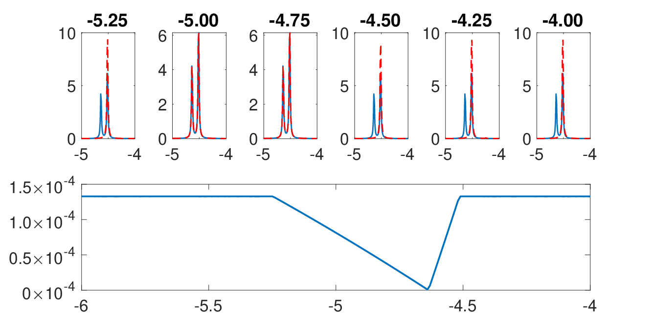
The reason behind this is as follows. Let us keep other poles fixed at their true values and let vary from to , and plot the landscape of the loss function in Fig. 3 (bottom panel). We can see that the loss function is highly nonconvex. When is outside the interval , the loss function is essentially flat. In fact, if , the optimized semidefinite matrix is a zero matrix. This will result in a vanishing gradient for (see Eq. 28), and therefore the optimization could not continue. In such an adversarial scenario, a random initialization of poles cannot recover the true pole locations.
III.2 Bosonic response functions
In order to demonstrate that the PES method is also applicable to bosonic response functions, let us consider the quantity of the Hubbard dimer model, which indicates the same-spin susceptibility for the -th site of the system. This function is also used in Schött et al. 2016 to test the performance of analytic continuation methods for bosonic functions. We use the Hubbard dimer example with the same parameters as in Section III.1 other than taking .
Let us use to denote the time-response function in the frequency domain. We are trying to fit the Matsubara data of into the following form:
| (33) |
where the quantities satisfies the semidefinite constraints Eq. 5 and the constraint
| (34) |
Here since we are only considering the time response function with respect to the -th site.
In the current physical system, the spectral function of has four peaks, with two on the positive half axis, and two on the negative half axis. In fact, is an odd function. Since the susceptibility is mirrored for negative frequencies, we only choose to plot the positive half axis. Note that since the Nevanlinna and Carathéodory continuation are not applicable to bosonic functions, we can only compare the PES method to the MaxEnt continuation method, for Matsubara data with different noise levels and . The result is shown in Fig. 4.

The MaxEnt method could not resolve the peaks of the bosonic response function under any noise level. We can see that when the noise level is small (), the PES method could recover both peaks on the positive half axis. When the noise level is large (), the PES method could only recover one peak. This means that the noise-robustness of PES method for bosonic functions are comparable to that for fermionic functions.
III.3 Band structure
We now applied the PES method to ab initio band structure calculations of solids. We use two data sets obtained from GW calculations: the matrix-valued Green’s functions for crystalline Si in the equilibrium geometry, previously analyzed in Ref. Fei et al. 2021b, and for AgI obtained with a relativistic exact two-component formulation in the one-electron approximation (x2c1e) Yeh et al. 2022a. The data have been obtained by fully self-consistent GW formulated in Gaussian Bloch orbitals, as described in detail in Ref. Yeh et al. 2022b. Both AgI and Si employ the gth-dzvp-molopt-sr basis VandeVondele and Hutter 2007 with gth-pbe pseudopotential Goedecker et al. 1996, using integrals generated by the PySCF package Sun et al. 2020 and a code based on ALPS Gaenko et al. 2017. Calculations are performed on a 6 6 6 grid Iskakov et al. 2020 and interpolated using a Wannier interpolation of Matsubara data Yeh et al. 2022b on 52 positive IR frequencies Shinaoka et al. 2017; Li et al. 2020 on a grid with 200 momentum points along a high-symmetry path. The broadening parameter of is larger than the temperature of and correlation effects.

The analytic continuation is conducted as follows. Since the number of orbitals is much larger than that in the Hubbard dimer example ( for silicon and for AgI), the computational cost will be too high if we conduct the analytic continuation for the entire matrix. Therefore we only implement the analytic continuation for the diagonal elements. The projection step is conducted on each diagonal entry separately with a fine grid of points. After the projection step, we estimate the poles of each diagonal entry using AAA algorithm, and then conduct the SDR fitting of each diagonal entry separately.
We conduct analytic continuation for Matsubara data with different noise levels and . The results of the spectral functions along a high symmetry path reveal the band structure, and are plotted in Fig. 5. We place a white marker in the plot if the corresponding component of the spectral function becomes negative to indicate that the result is unphysical.
Once again, we can see that Nevanlinna continuations could result in negative spectral functions even for the clean data, while Nevanlinna continuations combined with the causal projection can largely resolve the isuse of noise-sensitivity. PES method, ES method and the Nevanlinna continuation on projected data routine are all noise-robust. Even at a relatively large noise-level , the structure of the valence and conduction bands can be recovered. This means that our noise-robust analytic continuation methods could successfully retrieve information such as the band gap from Matsubara data even under a significant noise level.
IV Discussion
In this article, we have proposed a robust analytic continuation method called PES, consisting of the following three steps: causal projection, pole estimation and SDR fitting through bi-level optimization. The PES method is noise-robust, could deal with matrix-valued Green’s functions and is applicable to both fermionic and bosonic systems. As a by product, we also find that the causal projection could significantly improve the performance of noise-sensitive methods such as Nevanlinna and Carathéodory continuation. We have also demonstrated these properties with extensive numerical experiments.
Our current strategy of pole estimation is to perform AAA algorithm on the projected data. Note that the AAA algorithm is still an interpolation procedure can be susceptible to noise. The causal projection alleviates this drawback, and in practice it often provides a good enough initial guess for SDR fitting even in the noisy scenario. A better strategy to estimate the pole locations (e.g., by combining with the Prony method Ying 2022b) may still be helpful in improving the overall performance of the PES method. Moreover, the current SDP solver (SDPT3) can be computationally expensive when the number of variables is large. In such a case, more efficient solvers based on first-order methods may reduce the computational time in both the projection and the SDR fitting steps.
As we have shown, the PES method is useful for retrieving the excitation spectra of molecules and band structures in solids. These data feature multiple sharp peaks modeled by poles on the real axis. It could also be used to perform bath fitting in the Dynamical Mean Field Theory (DMFT) Mejuto-Zaera et al. 2020, and it is applicable in lattice gauge theory (for example, see Burnier and Rothkopf 2013; Tripolt et al. 2019). Broadened spectral functions that cannot be resolved into discrete peaks may be modeled by a relatively small number of poles away from the real axis. This would require modification of the definition of the causal space. Note that in the noisy scenario, it may be very difficult to distinguish the spectra described by a pole in the complex plane and the spectra due to many poles on or near the real axis. Therefore prior information such as the maximum number of complex poles and approximate pole locations may become necessary. This scenario will be investigated in future work.
Acknowledgment
This material is based upon work supported by the U.S. Department of Energy, Office of Science, Office of Advanced Scientific Computing Research and Office of Basic Energy Sciences, Scientific Discovery through Advanced Computing (SciDAC) program under Award Number DE-SC0022198 (Z.H.) and DE-SC0022088 (E.G.). The work is partially supported by the Air Force Office of Scientific Research under award number FA9550-18-1-0095 (L.L.). L.L. is a Simons Investigator. We thank Jiahao Yao, Lexing Ying, Yang Yu and Dominika Zgid for helpful discussions.
References
- Baker et al. (1996) G. A. Baker, G. A. Baker Jr, P. Graves-Morris, G. Baker, and S. S. Baker, Pade Approximants: Encyclopedia of Mathematics and It’s Applications, Vol. 59 George A. Baker, Jr., Peter Graves-Morris, vol. 59 (Cambridge University Press, 1996).
- Schött et al. (2016) J. Schött, I. L. Locht, E. Lundin, O. Grånäs, O. Eriksson, and I. Di Marco, Physical Review B 93, 075104 (2016).
- Jarrell and Gubernatis (1996) M. Jarrell and J. E. Gubernatis, Physics Reports 269, 133 (1996).
- Asakawa et al. (2001) M. Asakawa, Y. Nakahara, and T. Hatsuda, Progress in Particle and Nuclear Physics 46, 459 (2001).
- Levy et al. (2017) R. Levy, J. LeBlanc, and E. Gull, Computer Physics Communications 215, 149 (2017).
- Bryan (1990) R. Bryan, European Biophysics Journal 18, 165 (1990).
- Rothkopf (2020) A. Rothkopf, Data 5, 85 (2020).
- Sandvik (1998) A. W. Sandvik, Physical Review B 57, 10287 (1998).
- Vafayi and Gunnarsson (2007) K. Vafayi and O. Gunnarsson, Physical Review B 76, 035115 (2007).
- Fuchs et al. (2010) S. Fuchs, T. Pruschke, and M. Jarrell, Physical Review E 81, 056701 (2010).
- Shao and Sandvik (2022) H. Shao and A. W. Sandvik, Progress on stochastic analytic continuation of quantum monte carlo data (2022), eprint 2202.09870.
- Yoshimi et al. (2019) K. Yoshimi, J. Otsuki, Y. Motoyama, M. Ohzeki, and H. Shinaoka, Computer Physics Communications 244, 319 (2019).
- Motoyama et al. (2022) Y. Motoyama, K. Yoshimi, and J. Otsuki, Physical Review B 105, 035139 (2022).
- Fournier et al. (2020) R. Fournier, L. Wang, O. V. Yazyev, and Q. Wu, Physical Review Letters 124, 056401 (2020).
- Yoon et al. (2018) H. Yoon, J.-H. Sim, and M. J. Han, Physical Review B 98, 245101 (2018).
- Tomczak and Biermann (2007) J. M. Tomczak and S. Biermann, Journal of Physics: Condensed Matter 19, 365206 (2007).
- Dang et al. (2014) H. T. Dang, X. Ai, A. J. Millis, and C. A. Marianetti, Physical Review B 90, 125114 (2014).
- Gull and Millis (2014) E. Gull and A. J. Millis, Physical Review B 90, 041110 (2014).
- Kraberger et al. (2017) G. J. Kraberger, R. Triebl, M. Zingl, and M. Aichhorn, Physical Review B 96, 155128 (2017).
- Reymbaut et al. (2017) A. Reymbaut, A.-M. Gagnon, D. Bergeron, and A.-M. S. Tremblay, Phys. Rev. B 95, 121104 (2017).
- Kac and Krein (1974) I. S. Kac and M. G. Krein, Amer. Math. Soc. Transl 103, 1–18 (1974).
- Belyi et al. (2006) S. Belyi, S. Hassi, H. de Snoo, and E. Tsekanovskii, Linear algebra and its applications 419, 331 (2006).
- Fei et al. (2021a) J. Fei, C.-N. Yeh, and E. Gull, Physical Review Letters 126, 056402 (2021a).
- Fei et al. (2021b) J. Fei, C.-N. Yeh, D. Zgid, and E. Gull, Physical Review B 104, 165111 (2021b).
- Pick (1917) G. Pick, Mathematische annalen 78, 270 (1917).
- Khargonekar and Tannenbaum (1985) P. Khargonekar and A. Tannenbaum, IEEE Transactions on Automatic Control 30, 1005 (1985).
- Tannenbaum (1987) A. Tannenbaum, in 26th IEEE Conference on Decision and Control (IEEE, 1987), vol. 26, pp. 1635–1636.
- Doyle et al. (2013) J. C. Doyle, B. A. Francis, and A. R. Tannenbaum, Feedback control theory (Courier Corporation, 2013).
- Osborne and Smyth (1995) M. R. Osborne and G. K. Smyth, SIAM J. Sci. Comput. 16, 119 (1995).
- Golub and Pereyra (2003) G. Golub and V. Pereyra, Inverse problems 19, R1 (2003).
- Beylkin and Monzón (2005) G. Beylkin and L. Monzón, Applied and Computational Harmonic Analysis 19, 17 (2005).
- Ying (2022a) L. Ying, arXiv preprint arXiv:2202.09719 (2022a).
- Ying (2022b) L. Ying, arXiv preprint arXiv:2202.02670 (2022b).
- Nakatsukasa et al. (2018) Y. Nakatsukasa, O. Sète, and L. N. Trefethen, SIAM Journal on Scientific Computing 40, A1494 (2018).
- Mejuto-Zaera et al. (2020) C. Mejuto-Zaera, L. Zepeda-Núñez, M. Lindsey, N. Tubman, B. Whaley, and L. Lin, Physical Review B 101, 035143 (2020).
- Negele and Orland (1988) J. W. Negele and H. Orland, Quantum many-particle systems (Westview, 1988).
- Gesztesy and Tsekanovskii (2000) F. Gesztesy and E. Tsekanovskii, Mathematische Nachrichten 218, 61 (2000).
- Shohat and Tamarkin (1950) J. A. Shohat and J. D. Tamarkin, The problem of moments, vol. 1 (American Mathematical Society (RI), 1950).
- Akhiezer (2020) N. I. Akhiezer, The classical moment problem and some related questions in analysis (SIAM, 2020).
- Grant and Boyd (2014) M. Grant and S. Boyd, CVX: Matlab software for disciplined convex programming, version 2.1 (2014).
- Tibshirani (1996) R. Tibshirani, J. Royal Stat. Soc. B 58, 267 (1996).
- Candes et al. (2006) E. J. Candes, J. K. Romberg, and T. Tao, Communications on Pure and Applied Mathematics 59, 1207 (2006).
- Bach, Francis and Jenatton, Rodolph and Mairal, Julien and Obozinski, Guillaume (2012) Bach, Francis and Jenatton, Rodolph and Mairal, Julien and Obozinski, Guillaume (2012).
- Driscoll et al. (2014) T. A. Driscoll, N. Hale, and L. N. Trefethen, Chebfun guide (2014).
- Berrut and Trefethen (2004) J.-P. Berrut and L. N. Trefethen, SIAM Rev. 46, 501 (2004).
- Feynman (1939) R. P. Feynman, Physical review 56, 340 (1939).
- Nocedal and Wright (1999) J. Nocedal and S. J. Wright, Numerical optimization (Springer Verlag, 1999).
- Toh et al. (2012) K.-C. Toh, M. J. Todd, and R. H. Tütüncü, in Handbook on semidefinite, conic and polynomial optimization (Springer, 2012), pp. 715–754.
- Mehrotra (1992) S. Mehrotra, SIAM Journal on optimization 2, 575 (1992).
- Vandenberghe and Boyd (1996) L. Vandenberghe and S. Boyd, SIAM Rev. 38, 49 (1996).
- Jiang, Kaifeng and Sun, Defeng and Toh, Kim-Chuan (2012) Jiang, Kaifeng and Sun, Defeng and Toh, Kim-Chuan, SIAM J. Optim. 22, 1042 (2012).
- Nakatsukasa and Trefethen (2020) Y. Nakatsukasa and L. N. Trefethen, SIAM Journal on Scientific Computing 42, A3157 (2020).
- Yeh et al. (2022a) C.-N. Yeh, A. Shee, Q. Sun, E. Gull, and D. Zgid (2022a).
- Yeh et al. (2022b) C.-N. Yeh, S. Iskakov, D. Zgid, and E. Gull, Fully self-consistent finite-temperature in gaussian bloch orbitals for solids (2022b).
- VandeVondele and Hutter (2007) J. VandeVondele and J. Hutter, The Journal of Chemical Physics 127, 114105 (2007), eprint https://doi.org/10.1063/1.2770708.
- Goedecker et al. (1996) S. Goedecker, M. Teter, and J. Hutter, Phys. Rev. B 54, 1703 (1996).
- Sun et al. (2020) Q. Sun, X. Zhang, S. Banerjee, P. Bao, M. Barbry, N. S. Blunt, N. A. Bogdanov, G. H. Booth, J. Chen, Z.-H. Cui, et al., The Journal of Chemical Physics 153, 024109 (2020), eprint https://doi.org/10.1063/5.0006074.
- Gaenko et al. (2017) A. Gaenko, A. Antipov, G. Carcassi, T. Chen, X. Chen, Q. Dong, L. Gamper, J. Gukelberger, R. Igarashi, S. Iskakov, et al., Computer Physics Communications 213, 235 (2017), ISSN 0010-4655.
- Iskakov et al. (2020) S. Iskakov, C.-N. Yeh, E. Gull, and D. Zgid, Phys. Rev. B 102, 085105 (2020).
- Shinaoka et al. (2017) H. Shinaoka, J. Otsuki, M. Ohzeki, and K. Yoshimi, Phys. Rev. B 96, 035147 (2017).
- Li et al. (2020) J. Li, M. Wallerberger, N. Chikano, C.-N. Yeh, E. Gull, and H. Shinaoka, Phys. Rev. B 101, 035144 (2020).
- Burnier and Rothkopf (2013) Y. Burnier and A. Rothkopf, Phys. Rev. Lett. 111, 182003 (2013).
- Tripolt et al. (2019) R.-A. Tripolt, P. Gubler, M. Ulybyshev, and L. von Smekal, Computer Physics Communications 237, 129 (2019), ISSN 0010-4655.