UTHEP- 773
The Fokker-Planck formalism for closed bosonic strings
Nobuyuki Ishibashi** * e-mail: ishibashi.nobuyuk.ft@u.tsukuba.ac.jp
Tomonaga Center for the History of the Universe,
University of Tsukuba
Tsukuba, Ibaraki 305-8571, JAPAN
Every Riemann surface with genus and punctures admits a hyperbolic metric, if . Such a surface can be decomposed into pairs of pants whose boundaries are geodesics. We construct a string field theory for closed bosonic strings based on this pants decomposition. In order to do so, we derive a recursion relation satisfied by the off-shell amplitudes, using the Mirzakhani’s scheme for computing integrals over the moduli space of bordered Riemann surfaces. The recursion relation can be turned into a string field theory via the Fokker-Planck formalism. The Fokker-Planck Hamiltonian consists of kinetic terms and three string vertices. Unfortunately, the worldsheet BRST symmetry is not manifest in the theory thus constructed. We will show that the invariance can be made manifest by introducing auxiliary fields.
1 Introduction
For constructing a string field theory (SFT), we should specify a rule to cut worldsheets into fundamental building blocks, i.e. propagators and vertices. A few simple rules were proposed and SFTs for bosonic strings were constructed following these rules [1, 2, 3, 4]. Construction of an SFT for superstrings is more complicated because of the spurious singularities [5].
The worldsheets of closed strings describing scattering amplitudes are punctured Riemann surfaces. In mathematics, there exists a convenient way to decompose them into fundamental building blocks. On a Riemann surface with genus and boundaries or punctures, one can introduce a metric with constant negative curvature, if . Such a metric is called a hyperbolic metric and surfaces with hyperbolic metrics are called hyperbolic surfaces. With a hyperbolic metric, one can decompose the surface into pairs of pants with geodesic boundaries. It may be possible to consider the pair of pants as the fundamental building block of the surface.
The hyperbolic metric was used to construct SFT in [6, 7, 8], in which the kinetic term of the action was taken to be the conventional one
| (1.1) |
so that the propagators correspond to cylinders. The theories include infinitely many vertices besides the three string vertex and the Feynman graphs have nothing to do with the pants decomposition. In this paper, we would like to construct an SFT based on the pants decomposition. Namely, we will construct an SFT for closed bosonic strings regarding the pair of pants as the three string vertex and the cylinders with vanishing heights as the propagator, as depicted in Figure 1.
In such a theory, a state of string will correspond to a boundary of a pair of pants. Accordingly, the string field should be labeled by an element of the Hilbert space of the first quantized strings and the length of the boundary. The external states of the scattering amplitudes are regarded as the limit of such states. The off-shell amplitudes may correspond to Riemann surfaces which have geodesic boundaries with fixed lengths and will be expressed by integrals over the moduli spaces of such surfaces.
Unfortunately, such an approach suffers from a problem addressed in [9] (section IV. E). The three string vertex will be given by the correlation function of the worldsheet theory on hyperbolic pants with the boundary lengths specified. Suppose that one calculates the one loop one point function following the conventional Feynman rules. The amplitude corresponds to the worldsheet in Figure 2 and we should integrate over the length and the twist angle . By doing so, the fundamental domain of the modular group is covered infinitely many times, as will be seen in section 4.3. The same happens for all the other amplitudes. Therefore, the conventional Feynman rule with the vertex and the propagator in Figure 1 does not yield the correct amplitudes.
In order to overcome this problem, we formulate the theory using the Mirzakhani’s scheme [10, 11] for computing integrals over moduli space of bordered Riemann surfaces. Mirzakhani derived a recursion relation for the volume of the moduli space. Applying her method to the off-shell amplitudes of closed bosonic strings, we derive a recursion relation satisfied by these amplitudes.
As was pointed out in [12, 13], Mirzakhani’s recursion relation is related to the loop equation of minimal string theory. On the other hand, the loop equations for minimal strings can be described by an SFT via the Fokker-Planck formalism [14, 15]. We will show that the recursion relation of the off-shell amplitudes can be described by an SFT using the Fokker-Planck formalism. The Fokker-Planck Hamiltonian consists of kinetic terms and three string vertices. One can develop perturbation theory which does not suffer from the above mentioned problem. Unfortunately, the worldsheet BRST symmetry is not manifest in the SFT thus constructed. We will show that we can make the invariance manifest by introducing auxiliary fields.
The organization of this paper is as follows. In section 2, we define the off-shell amplitudes of closed bosonic string theory based on the moduli space of bordered Riemann surfaces. In section 3, we derive recursion relations satisfied by the off-shell amplitudes. In section 4, we prove that the off-shell amplitudes defined in section 2 can be derived from the Fokker-Planck formalism for string fields. We show that the solution of the recursion relations in section 3 satisfies the Schwinger-Dyson equation derived from the Fokker-Planck Hamiltonian. In section 5, we modify the theory by introducing auxiliary fields and make it manifestly BRST invariant. Section 6 is devoted to discussions and comments. In Appendix A, we present formulas for the local coordinates on hyperbolic pants. In appendix B, we prove the BRST identity.


2 Off-shell amplitudes
The off-shell amplitudes of the theory we will study should correspond to hyperbolic surfaces which have geodesic boundaries with fixed lengths. In this section, we would like to define such amplitudes. The formulation is a modification of the conventional ones [4, 16, 17, 18].
2.1 The moduli space
Let with be a genus hyperbolic surface with geodesic boundaries (labeled by an index ) whose lengths are . Cutting the surface along non-peripheral simple closed geodesics, we can decompose it into pairs of pants . There are many choices for such decomposition and here we pick one. The hyperbolic structure of the surface is specified by the lengths of the non-peripheral simple closed geodesics and the way how boundaries of ’s are identified. Therefore the hyperbolic structure of can be parametrized by the Fenchel-Nielsen coordinates , where are the lengths of the nonperipheral boundaries of and denotes the twist parameters which specify how boundaries of different pairs of pants are identified. The Teichmüller space corresponds to the region . A volume form on called the Weil-Petersson volume form is given by
does not depend on the choice of the pants decomposition. The moduli space is defined as
where denotes the mapping class group. The Fenchel-Nielsen coordinates can be used as local coordinates on . We will define the off-shell amplitudes as integrals over . The space of all inequivalent hyperbolic structures on a surface is the same as that of the complex structures. Hence the definition of the off-shell amplitudes here can be regarded as the traditional one for the case where the lengths of the external strings are specified.
2.2 -ghost insertions
Let us consider an element of . One can attach a flat semi-infinite cylinder to each boundary [8] as depicted in Figure 3 and obtain a punctured Riemann surface. The cylinder is conformally equivalent to a disk with a puncture. Let be a local coordinate on the -th disk such that corresponds to the region , the flat metric is given as
and the -th puncture corresponds to . By these conditions, is fixed up to a phase rotation. can be expressed as a function of a local coordinate on . is holomorphic in a neighborhood of .
In this way, from , we obtain a punctured Riemann surface with local coordinates around punctures, which are specified up to phase rotations. To thus obtained, one can associate a surface state, picking a local coordinate as above for each . Let us denote this surface state by . By definition, we have
| (2.1) |
where denotes the operator corresponding to the state and denotes the correlation function on . Under a phase rotation , transforms as
The correlation function is invariant under the phase rotation, if

In order to define the amplitudes, we need to construct a top form on the moduli space from the -ghost. A deformation of the hyperbolic structure of a surface induces that of the complex structure. Therefore we can construct the -ghost insertion corresponding to a tangent vector of , following the procedure given in [4, 16, 19, 18]. Let be a local coordinate on the pair of pants , such that the hyperbolic metric on is in the form
Each boundary of is either shared by another pair of pants or is equal to one of the boundaries of . In the former case, the local coordinate on and are related by
| (2.2) |
in a neighborhood of . If the boundary of coincides with , and are related by
| (2.3) |
in a neighborhood of . The transition functions describe the moduli of .
Suppose that under an infinitesimal change of moduli, change as
and we obtain
in a neighborhood of respectively. One can take to be holomorphic in neighborhoods of boundaries of and smooth inside. For such , we define
| (2.4) |
Here the integration contours are taken so that they run along keeping on the left for .
For our purpose, we need to make the formulas (2.2), (2.3) and (2.4) more explicit. itself is a hyperbolic surface with three boundaries and by attaching flat semi-infinite cylinders to the boundaries as above, we get a three punctured sphere with local coordinates . Therefore is conformally equivalent to where are the disks corresponding to the cylinders. We choose the local coordinate on to be the complex coordinate on such that the three punctures are at . The explicit forms of are given in [20, 21], which are presented in appendix A. There is a freedom in choosing which of corresponds to each boundary of , but (A.3) implies ’s are related by transformation of and a phase rotation and the choice does not change the result. If the boundary of coincides with , we can take to be equal to . Then the explicit form of (2.3) becomes
| (2.5) |
should coincide with and for some and we obtain the explicit form of (2.2) as
| (2.6) |
where is the twist angle.
We take the Fenchel-Nielsen coordinates on . Changes of the transition functions (2.5) and (2.6) under the variation describe those of the hyperbolic structure of . If is the length of , . For , we can take
for , in neighborhoods of boundaries of respectively. Therefore we define
| (2.7) |
Here for in each term is chosen so that the relevant component of the boundary corresponds to . For , we define
| (2.8) |
where for is chosen so that coincides with . The contours run along so that lies to its left for .
In the same way, for a pair of pants one of whose boundary coincides with , we define
| (2.9) |
2.3 Off-shell amplitudes
Now we define the connected loop point amplitude by
| (2.10) |
Here is defined so that
holds for any , with
| (2.11) |
The factor is due to the fact that has a symmetry. The state is taken to be an element of which consists of the states satisfying
| (2.12) |
where .
is defined by using the Fenchel-Nielsen coordinate associated to a pants decomposition of . We should check if the amplitude (2.10) does not depend on the choice of the pants decomposition. Suppose that we have two pants decompositions, in which is decomposed into pairs of pants and . Let and be the local coordinates on respectively. There should be a function holomorphic on such that
If a boundary of coincides with , we have functions such that
| (2.13) |
in a neighborhood of . Suppose that under an infinitesimal change of moduli, change as
We can derive
| (2.14) | |||||
| (2.15) |
(2.14) implies
If we take to be holomorphic in neighborhoods of the boundaries of respectively, we get
Therefore the -ghost insertion (2.4) satisfies
| (2.16) |
if and corresponds to the same change of moduli.
Let be the Fenchel-Nielsen coordinates associated to the two different pants decompositions. Using (2.16), we may be able to express in terms of . In doing so, there is one thing one should be careful about. In defining , we have taken the coordinate on to be , if coincides with a boundary of . If one of boundaries of coincides with ,
should hold with some . Here is a real function of moduli. If we fix in (2.13) to be , (2.15) implies
Therefore the relations between and should be
Here denotes acting on the -th Hilbert space. Substituting these into the amplitude (2.10), we can see that it is independent of the pants decomposition, if satisfy the condition (2.12).
By the BRST identity proved in appendix B, we have
| (2.17) |
and the amplitude is BRST invariant if one treats the boundary contributions appropriately. By construction, exists for .
The amplitude (2.10) is not something we usually deal with in string theory. In the limit , coincides with the moduli space of punctured Riemann surfaces and become the Fenchel-Nielsen coordinates on . Therefore
| (2.18) |
is equal to the on-shell amplitude when are taken to be on-shell physical states. In section 5, we will show that the off-shell amplitudes of the kind studied in [22, 23, 24] can also be derived in our formalism.
3 A recursion relation of the off-shell amplitudes
Given a propagator, one can construct the string field action which reproduces the off-shell amplitudes defined in the previous section order by order in the string coupling constant If we take the propagator to be the one depicted in Figure 1, we run into the difficulty mentioned in introduction. In this paper, as a workaround, we construct an SFT by studying equations satisfied by the off-shell amplitudes.
In order to calculate the right hand side of (2.10), we need to specify the integration region in terms of the Fenchel-Nielsen coordinates. However no concrete description of the fundamental domain of the mapping class group in is known in general. Mathematicians were trying to calculate the the Weil-Petersson volume of defined by22 2 There are two conventions for due to the presence of symmetry. Here we adopt (3.1) so as to make (3.11) look simple.
| (3.1) |
and encounter the same problem. Mirzakhani discovered [10, 11] a way to overcome this difficulty. In this section, we would like to explain her method (for reviews, see for instance [7, 25, 26]) and apply it to the off-shell amplitudes.
3.1 Mirzakhani’s scheme
Mirzakhani’s idea is to transform an integral over into the one over its covering space. Suppose are are manifolds and
is a covering map. Let be a volume form on , and we define to be the pull back, i.e.
For a function on , one can define the push forward by
Then
| (3.2) |
holds.
Eq. (3.2) can be used to calculate the volume of the moduli space , for example. We take to be and to be the following space of pairs
The set of simple closed geodesics on is a discrete set with infinitely many elements and a mapping class group orbit. can be described by the pair where is the length of and is the twist parameter corresponding to it. corresponds to the region
with . The projection can be defined by
and for , we have
If one takes the function to be a function of , the value of at becomes
where the sum is over the set of simple geodesics on . In [27], McShane proved that for ,
| (3.3) |
holds. (3.3) is called the McShane identity. For this choice of , (3.2) becomes
| (3.4) |
and we get the volume of .
Mirzakhani generalized this procedure to general , by discovering a generalization of the McShane identity. For , let be the boundaries so that the lengths of are respectively. The generalized McShane identity derived in [10] is
| (3.5) |
where
| (3.6) | |||||
| (3.7) |
and are the lengths of respectively. For , >0 and
| (3.10) |
Multiplying (3.5) by and integrating it over , one obtains the Mirzakhani’s recursion relation:
| (3.11) | |||||
which holds for . The sum here means the sum over such that33 3 Here we consider as unordered subsets of .
| (3.12) |
With the information , , it is possible to calculate for all the other by the recursion relation (3.11).
3.2 Recursion relation of the off-shell amplitudes
A recursion relation of the off-shell amplitudes (2.10) is derived in the same way as the Mirzakhani’s recursion relation. Multiplying (3.5) by and integrating it over , we obtain
| (3.13) |
The left hand side yields
Here we restrict ourselves to the case . We will rewrite the terms on the right hand side by using the formula (3.2). Let us first consider the integral
| (3.14) |
In order to unfold this integral, we take to be and to be the space of pairs
The set of possible on is exactly and is a mapping class group orbit. can be described by the triple where is the twist parameter corresponding to and is the complement of the pair of pants bounded by with . corresponds to the region
with . The projection can be defined by
and for , we have
where is the Weil-Petersson volume form on .
Now, if one takes
(3.2) becomes
| (3.15) |
Therefore (3.14) is obtained by evaluating the left hand side of (3.15).

Let us consider a pants decomposition of such that one pair of the pants is with boundaries (Figure 4). We denote this pair of pants by and the adjacent one by . Based on the pants decomposition we define the Fenchel-Nielsen coordinates such that . Cutting along , we get a three holed sphere and . inherits the pants decomposition of . Then can be expressed as
| (3.16) |
where denotes the form on defined through (2.11).
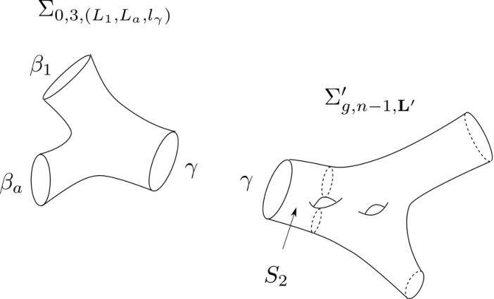
can be generated by gluing a pair of pants and (Figure 5) using the plumbing fixture relation (2.6). Hence the correlation function on the right hand side of (3.16) can be factorized into those on and . Let be a basis of the Hilbert space of the worldsheet theory of the strings and be the conjugate state of such that
Here is the BPZ conjugate of and is the ghost number of . Then we have
| (3.17) |
where
denotes the ghost number of and denotes the twist angle. The factor is due to the fact that has a symmetry for .
Substituting (3.16) and (3.17) into (3.15), we can see that the second term on the right hand side of (3.13) becomes
| (3.18) |
with .
(3.18) implies that it will be convenient to consider the recursion relation of the amplitudes of the form
| (3.19) |
Here the indices take values and
| (3.20) |
for in (3.20) denotes the pair of pants which has a boundary corresponding to the -th external line in a pants decomposition of . depends on the choice of the pants decomposition, because it corresponds to the variation with fixed. However, and the amplitude in (3.19) is independent of the choice of .
(3.18) can be recast into
| (3.21) |
We simplify the formula by introducing the following notation. The external states are labeled by (for ), , and . We denote these collectively by and rewrite (3.21) in the following way:
| (3.22) |
where
and for and
The integral
| (3.23) |
on the right hand side of (3.13) can be dealt with in the same way. In this case, there can be topologically distinct configurations of the pair in as depicted in Figure 6. They belong to different mapping class group orbits. For each orbit, we take to be the space of the combination , where is in the orbit and express the contribution to (3.23) by an integral over . The amplitudes are factorized as in Figure 7. A formula similar to (3.22) can be derived for each contribution.


Putting everything together, we can see that (3.13) is transformed into
| (3.24) | |||||
which holds for . Here are ordered sets of indices with elements respectively. The sum means the sum over such that
| (3.25) |
is the sign which will appear when we change the order of the product to , if we regard the indices as Grassmann numbers with Grassmannality of the corresponding string state.
Eq.(3.24) can be made more tractable by introducing . Since we define the amplitudes for surfaces with , amplitudes for do not exist. We here introduce a fictitious amplitude
where
which satisfies
Taking this into account, we can turn (3.24) into
| (3.26) | |||||
which holds for or . Here the summation is over such that
Let us check if (3.26) is valid for . For , (3.26) becomes44 4 Notice that does not exist.
| (3.27) |
The first term on the right hand side of (3.26) is introduced so that holds. For , we have
where denotes the Grassmannality of . Substituting (3.10) into this, we obtain
| (3.28) |
Notice that is a point and (3.19) implies
| (3.29) |
which is consistent with the above equation. For , (3.26) becomes
| (3.30) | |||||
On the other hand, can be given as
The integral on the last line can be unfolded by using the McShane identity and we get exactly (3.30).
3.3 The solution of the recursion relation
The recursion relation (3.24) is derived from the properties of the off-shell amplitudes . Conversely, can be derived by solving the equation (3.24).
is the order contribution to the point amplitude. (3.26) can be solved order by order in , because the right hand side of (3.26) consists of lower order terms compared with the on the left hand side. For example, the equation for becomes (3.28) and the solution is (3.29) because is defined for . (3.26) can be solved in the same way for general . The solution is unique, because is defined for . This unique solution should coincide with the in (3.19). Therefore the equation (3.26) can be used to derive the off-shell amplitudes of closed bosonic string theory.
For later convenience, let us define the generating functional of the off-shell amplitudes:
| (3.31) |
is taken to have the same Grassmannality as that of . It is straightforward to show that the recursion relation (3.26) is equivalent to the following identity:
| (3.32) | |||||
Here all the functional derivatives are the left derivatives.
4 The Fokker-Planck formalism
In this section, we would like to develop the Fokker-Planck formalism for the string theory from which we can derive the recursion relation (3.26) through the Schwinger-Dyson equation.
4.1 The Fokker-Planck formalism for conventional field theory
Let be a scalar field with action S[. The Euclidean correlation functions are defined by
| (4.1) |
where
| (4.2) |
In order to describe this quantum field theory, we consider a system governed by the following Fokker-Planck equation:
| (4.3) |
Here is the Fokker-Planck Hamiltonian defined by
| (4.4) |
It is possible to show that for a solution of (4.3) with an appropriate initial condition,
holds. The Fokker-Planck equation with the Fokker-Planck Hamiltonian (4.4) appears in the context of stochastic quantization [28] where coincides with the fictitious time.
The Fokker-Planck Hamiltonian can be realized as an operator acting on a Hilbert space. Let be operators satisfying the commutation relations
and be states satisfying
Then
with
gives a solution to (4.3) with initial condition . Assuming that this is a good initial condition, we get
| (4.5) |
The correlation function in (4.1) is given by
In [14], a string field theory for the minimal string theory using this kind of operator formalism was proposed. The string fields are labeled by the length of the string and we define the operators accordingly. The Fokker-Planck Hamiltonian is given by
where is the disk amplitude for the minimal string theory55 5 The correspondence between our notation and that in [14] is given by . The correlation functions of the string fields are given by
| (4.6) |
One can prove that the correlation functions thus defined coincide with the loop amplitudes of the minimal string theory, in the following way. In order for the limit (4.6) to exist,
| (4.7) |
should hold. (4.7) yields the Schwinger-Dyson equation satisfied by the correlation functions of the minimal string theory. It can be shown that the loop equation of the minimal string theory is equivalent to this Schwinger Dyson equation. Moreover this string field theory can be derived from the stochastic quantization of the one matrix model [15]. The Fokker-Planck formalism was applied to construct string field theories for general minimal string theories in [29, 30, 31].
4.2 The Fokker-Planck Hamiltonian for closed bosonic strings
In [12], it was shown that Mirzakhani’s recursion relation (3.11) is a special case of random matrix recursion relations. In [13], (3.11) is identified with a limit of the loop equation of the minimal string theory. Since minimal string theory is a close cousin of the one, it is possible to develop the Fokker-Planck formalism of string field theory corresponding to (3.11). The recursion relation in (3.24) is a (not so close) cousin of (3.11), it is conceivable that the same approach is applicable to this equation. In this subsection, we would like to show that this is the case.
We introduce operators which satisfy the commutation relations
Here we define
Let be states which satisfy
| (4.8) |
We define the correlation functions of ’s as
| (4.9) |
with Hamiltonian
| (4.10) | |||||
As we will see, the right hand side of (4.9) can be calculated perturbatively with respect to . We define the connected correlation functions in the usual way and they can be expanded as
It is possible to show that
| (4.11) |
holds.
In order to prove (4.11), we define the generating functional of the connected correlation functions
| (4.12) |
such that
Since the limit of exists, we have66 6 (4.13) can be proved perturbatively in .
| (4.13) |
Using (4.8), we get the following equation from (4.13):
| (4.14) | |||||
It is possible to solve (4.14) order by order in and obtain . For example, at , (4.14) implies
Since is defined for , we obtain the unique solution
| (4.15) |
In general, (4.14) implies an equation in which is expressed in terms of lower order correlation functions. Since is defined for , one can solve the equation and the solution is unique. Hence all the coefficients of the expansion (4.12) is uniquely fixed by (4.14). On the other hand,
| (4.16) |
yields a solution to (4.14) because satisfies (3.32). Since the solution of (4.14) should be unique, we obtain (4.11).
(4.16) implies that satisfies the equation (3.32), which can be expressed as
| (4.17) |
in the Fokker-Planck formalism. Here
| (4.18) | |||||
and we have
Since every ket vector is expressed as a linear combination of states of the form
(4.9) means that is expressed as
In the same way, we can deduce from (4.13), (4.17)
| (4.19) |
4.3 String field action
In the case of conventional field theory, the Fokker-Planck formalism is an alternative to the path integral formalism. Let us discuss if the theory we have can be formulated using a path integral with action . It is possible to define the weight following (4.5):
From (4.19), we obtain an equation for :
| (4.20) |
Using (3.10), the last term on the right hand side of (4.20) is expressed as
The integrand of the first term on the right hand side coincides with that of , but the integration region includes infinitely many fundamental domains of the mapping class group. The second term is equal to . Therefore the last term on the right hand side of (4.20) may be given as
and divergent. Hence the equation (4.20) is not well-defined.
Still, (4.20) can be solved formally order by order in and we get
| (4.21) |
This should be the action which yields the off-shell amplitudes with the propagator . Let us compute the one loop one point function using the path integral formalism. The contribution from the three string vertex becomes
and diverges. The contribution from divergent term in the action cancels this divergence and we get the correct answer . This pattern seems to continue forever. If one computes the four point amplitude using the three string vertex in (4.21), one gets a divergent result. The four string vertex cancels the divergence and make the amplitude finite.
Therefore, the Fokker-Planck formalism is necessary for a well-defined formulation of the theory in our setup. On the other hand, the formally defined action (4.21) will be useful in studying various aspects of our formulation.
4.4 SFT notation
In order to discuss various properties of the theory, it is more convenient to express the Fokker-Planck Hamiltonian (4.10) in terms of the variables in the Hilbert space of strings. Let us define
| (4.22) | |||||
| (4.23) |
The string fields are taken to satisfy
| (4.24) |
where consists of the states satisfying
where . We also impose the reality condition [4, 32]
| (4.25) |
The reality condition for will not be so simple, as is always the case in the Fokker-Planck formalism. Conditions (4.24) and (4.25) have been implicitly assumed in the previous subsection.
Notice that are Grassmann even. They satisfy the canonical commutation relation
| (4.26) |
where
is the reflector and
The states satisfy
In terms of these string fields, the Fokker-Planck Hamiltonian (4.10) is expressed as
| (4.27) | |||||
where
and the sum over repeated indices is understood. and are given by
and the correlation functions of are expressed as
| (4.28) |
The correlation functions can be calculated perturbatively. The Euclidean action corresponding to the Fokker-Planck Hamiltonian (4.27) becomes
| (4.29) |
where
satisfy the boundary conditions
The correlation functions are expressed as
| (4.30) |
using the path integral. To develop the perturbation theory, we decompose the action as , and we get propagators by Wick’s theorem:
With the propagators and the vertex, it is straightforward to compute (4.30). By construction, the results are given by the integral
unfolded by Mirzakhani’s method. The integrations can be done taking care of the contributions from the boundaries of the moduli space appropriately.
5 BRST invariant formulation
With the Fokker-Planck formalism developed in the previous section, one can express the off-shell amplitudes of the bosonic string theory. In order to describe the string theory, we need the BRST symmetry on the worldsheet to specify which states of strings are physical. Unfortunately, the Fokker-Planck Hamiltonian (4.27) and the action (4.29) are not invariant under the BRST symmetry, although the amplitudes are. We will modify the action (4.29) so that the BRST symmetry becomes manifest in our formalism.
5.1 BRST transformation
As is proved in appendix B, satisfies the BRST identity
| (5.1) |
Integrating this over , we obtain
| (5.2) |
(5.2) implies that the correlation functions of is invariant under
| (5.3) |
with a Grassmann odd parameter . This can be identified with the BRST transformation of . It is easily checked that the two point function
is also BRST invariant. The transformation of the is fixed by requiring that the commutation relation (4.26) is invariant and we obtain
| (5.4) |
The generator of the transformation is given by
which satisfies
| (5.5) |
5.2 The BRST variation of
Although the correlation functions are invariant under (5.3), the Hamiltonian (4.27) is not. The BRST variations of the correlation functions which appear on the right hand side of (4.27) yield total derivatives with respect to the length variables, but they come with the coefficients and do not vanish upon integration.
5.3 BRST invariant formulation
Although does not vanish, (5.7) and (5.8) implies that it consists of “null” quantities. Using this fact, we will make the theory manifestly invariant under the BRST transformation by introducing auxiliary fields.
We modify the Euclidean action (4.29) by adding terms involving auxiliary fields as follows:
| (5.9) | |||||
Here is equal to ) with replaced by classical fields respectively. and are taken to satisfy the boundary conditions
is invariant under the BRST transformation
The correlation functions are defined by
| (5.10) |
We would like to show that the correlation functions in this BRST invariant theory coincide with those given in (4.30). The numerator of (5.10) is computed as
The terms on the right hand side vanish because of (5.7) and (5.8), and this becomes
The denominator is evaluated in the same way and we obtain
Therefore the correlation function (5.10) coincides with (4.30).
Now the theory is invariant under the BRST symmetry, we regard the BRST invariant quantities as physical. One type of BRST invariant observable is of the form
for satisfying
As we mentioned in section 2,
gives the on-shell amplitude if we take to be on-shell physical states.
Another type of BRST invariant observable would be of the form
| (5.11) |
with . The amplitude
| (5.12) |
for these observables is in the form of an integration over the moduli space of complex structures of Riemann surfaces with boundaries. Therefore it is natural to take to be
where is the boundary state corresponding to some D-brane configuration. For example, taking the states to be the point like string state with appropriate ghost part, we obtain the off-shell amplitudes of the kind studied in [22, 23, 24]. Such amplitudes involve the external leg contributions coming from the integration region . Indeed, using (A.5), the contribution of for can be approximated as
This type of observable is suitable for studying mass renormalization [33, 34].
6 Discussions
In this paper, we have constructed a string field theory for closed bosonic strings based on the pants decomposition of hyperbolic surfaces. In such a setup, the Fokker-Planck formalism is indispensable as discussed in section 4.3. We have introduced auxiliary fields to make the theory manifestly BRST invariant. The action (5.9) we obtain consists of kinetic terms and three string vertices.
There are many interesting points that deserve further study. The most obvious one would be to construct an SFT for superstrings based on the same idea. It is straightforward to generalize our formalism to Type 0 superstring case, using the supersymmetric version of (3.5) derived in [35]. We will present the results elsewhere.
The formulation we get in section 5 is invariant under the worldsheet BRST symmetry. We should clarify the meaning of this symmetry from the point of view of string fields. In ordinary formulation of SFT, the worldsheet BRST symmetry is utilized to define the gauge or BRST transformation for string fields which is nonlinear with respect to these fields. In our case, the worldsheet BRST symmetry will not be related to the gauge or BRST symmetry of the string fields in the usual way, because the theory is not based on a triangulation of the moduli space. The similarity between the structure of our formalism and that of the covariantized light-cone SFT [36] may provide a clue to this problem.
Our formalism is based on the one constructed for minimal strings. In the minimal string case, the operator corresponding to in (4.18) becomes
and satisfies
| (6.1) |
Eq.(6.1) is equivalent to the Virasoro constraints [37, 38]. satisfies an algebra
| (6.2) |
which serves as the integrability condition of (6.1). Laplace transforming (6.2), we obtain the Virasoro algebra. We are not sure if satisfies a similar algebra. Exploring the algebra of will be crucial in understanding the structure of the theory. It may be also important to point out that one can take the Fokker-Planck Hamiltonian to be
instead of (5.6). Here is a function of satisfying for . The recursion relation can be derived from this modified Hamiltonian. Such a Hamiltonian was constructed in [39] in the minimal string case.
The classical equation of motion for string fields can be derived in our formalism. It is possible to assign the target space ghost number such that [4]
The fields with can be considered as the classical fields. Although the action is not well-defined, eq.(4.20) implies that the equation
may be identified with the classical equation of motion for string fields. In the BRST invariant formulation in section 5, this equation coincides with
| (6.3) |
under the conditions
| (6.4) |
For BRST invariance, we may also have to impose
| (6.5) |
Indeed (6.3) (6.4) and (6.3) solves the equation of motion derived from the action (5.9), if the auxiliary fields vanish.
Acknowledgments
Part of this work was presented at the workshop “Nonperturbative Analysis of Quantum Field Theory and its Applications” held at Osaka University. The author would like to thank the organizers for their warm hospitality and S. Aoki, S. Nishigaki and Y. Sumino for comments. This work was supported in part by Grant-in-Aid for Scientific Research (C) (18K03637) from MEXT.
Appendix A Hyperbolic metric on the three holed sphere
Let us consider a hyperbolic pants whose boundaries are geodesics. The pair of pants is conformally equivalent to where are disks around respectively. We take the length of to be . Around , a local coordinate is taken so that the metric becomes
The boundary corresponds to
where is an integer. can be expressed as a function of the complex coordinate on . Although have singularities in , it is well-defined around and the three-holed sphere corresponds to the region
The explicit forms of are given by[20, 21]
| (A.1) |
where
| (A.2) |
and
Notice that
| (A.3) |
hold. Attaching flat semi-infinite cylinders to the boundaries of the three holed sphere, we get a surface conformally equivalent to a three punctured sphere. The local coordinates on the cylinders are given by
| (A.4) |
up to a phase rotation and the metrics on the cylinders become
Notice that gives geodesics connecting the boundary components and perpendicular to them. Therefore become the basepoints which are used to define the twist parameters of the Fenchel-Nielsen coordinates [40].
For studying various properties of the amplitudes, it is useful to examine the limits of the formula (A.4). Since the behavior does not depend on because of (A.3), we consider the case . In the limit , (A.2) implies
where
and . From (A.1) and (A.4), we get
should be taken [20] so that and we eventually obtain
| (A.5) |
The limit can be obtained from the Fuchsian equation. We get
| (A.6) |
Appendix B BRST identity
In this appendix, we would like to prove
| (B.1) |
where
It is straightforward to derive (2.17) and (5.1) from (B.1).
Decomposing into pairs of pants, can be expressed in terms of . In order to prove (B.1), we will study some of the properties of . satisfies
Here we take the local coordinate on to be the in appendix A and is given in (A.4). We introduce the twist angles by deforming as
so that we have
| (B.2) |
where
(B.2) implies
which can be regarded as the definition of the state .
Following the formula (2.4), we define
with
Here are the stress tensors of the worldsheet theory and we have
| (B.3) |
with
It is possible to show that for any state ,
holds. Hence we obtain
| (B.4) | |||||
We can also define
and it is easy to prove
| (B.5) |
and satisfy the following commutation relations:
| (B.6) |
Other cases can be proved by using (B.7). Let us consider the next simplest case . The surface state can be expressed as
| (B.8) | |||||
Using this, we obtain
In going from the first line to the second line, we have used
| (B.10) |
Using (B.7), we eventually get
| (B.11) | |||||
The proof for all the other cases goes in the same way. We use induction with respect to . So far we have shown (B.1) for . Assuming that (B.1) is true for , let us prove (B.1) for . can be expressed by and surface states with by factorizing the surface as in Figure 5 or Figure 7. Using the induction hypothesis, we obtain (B.1) for in the same way as we did for .
References
- [1] M. Kaku and K. Kikkawa, “The field theory of relativistic strings. i. trees,” Phys. Rev. D 10 (1974) 1110.
- [2] E. Witten, “Noncommutative geometry and string field theory,” Nucl. Phys. B 268 (1986) 253–294.
- [3] T. Kugo and B. Zwiebach, “Target space duality as a symmetry of string field theory,” Prog. Theor. Phys. 87 (1992) 801–860, arXiv:hep-th/9201040.
- [4] B. Zwiebach, “Closed string field theory: Quantum action and the b-v master equation,” Nucl. Phys. B 390 (1993) 33–152, arXiv:hep-th/9206084.
- [5] C. de Lacroix, H. Erbin, S. P. Kashyap, A. Sen, and M. Verma, “Closed superstring field theory and its applications,” Int. J. Mod. Phys. A 32 (2017) no. 28n29, 1730021, arXiv:1703.06410 [hep-th].
- [6] S. F. Moosavian and R. Pius, “Hyperbolic geometry and closed bosonic string field theory. part i. the string vertices via hyperbolic riemann surfaces,” JHEP 08 (2019) 157, arXiv:1706.07366 [hep-th].
- [7] S. F. Moosavian and R. Pius, “Hyperbolic geometry and closed bosonic string field theory. part ii. the rules for evaluating the quantum bv master action,” JHEP 08 (2019) 177, arXiv:1708.04977 [hep-th].
- [8] K. Costello and B. Zwiebach, “Hyperbolic string vertices,” JHEP 02 (2022) 002, arXiv:1909.00033 [hep-th].
- [9] E. D’Hoker and D. H. Phong, “The geometry of string perturbation theory,” Rev. Mod. Phys. 60 (1988) 917.
- [10] M. Mirzakhani, “Simple geodesics and weil-petersson volumes of moduli spaces of bordered riemann surfaces,” Invent. Math. 167 (2006) no. 1, 179–222.
- [11] M. Mirzakhani, “Weil-petersson volumes and intersection theory on the moduli space of curves,” J. Am. Math. Soc. 20 (2007) no. 01, 1–24.
- [12] B. Eynard and N. Orantin, “Weil-petersson volume of moduli spaces, mirzakhani’s recursion and matrix models,” arXiv:0705.3600 [math-ph].
- [13] P. Saad, S. H. Shenker, and D. Stanford, “Jt gravity as a matrix integral,” arXiv:1903.11115 [hep-th].
- [14] N. Ishibashi and H. Kawai, “String field theory of noncritical strings,” Phys. Lett. B 314 (1993) 190–196, arXiv:hep-th/9307045.
- [15] A. Jevicki and J. P. Rodrigues, “Loop space Hamiltonians and field theory of noncritical strings,” Nucl. Phys. B 421 (1994) 278–292, arXiv:hep-th/9312118.
- [16] A. Sen, “Off-shell amplitudes in superstring theory,” Fortsch. Phys. 63 (2015) 149–188, arXiv:1408.0571 [hep-th].
- [17] T. Erler, “Four lectures on closed string field theory,” Phys. Rept. 851 (2020) 1–36, arXiv:1905.06785 [hep-th].
- [18] H. Erbin, String Field Theory: A Modern Introduction, vol. 980 of Lecture Notes in Physics. 3, 2021.
- [19] J. Polchinski, String theory. Vol. 1: An introduction to the bosonic string. Cambridge Monographs on Mathematical Physics. Cambridge University Press, 12, 2007.
- [20] L. Hadasz and Z. Jaskolski, “Classical liouville action on the sphere with three hyperbolic singularities,” Nucl. Phys. B 694 (2004) 493–508, arXiv:hep-th/0309267.
- [21] A. H. Fırat, “Hyperbolic three-string vertex,” JHEP 08 (2021) 035, arXiv:2102.03936 [hep-th].
- [22] A. G. Cohen, G. W. Moore, P. C. Nelson, and J. Polchinski, “An off-shell propagator for string theory,” Nucl. Phys. B 267 (1986) 143–157.
- [23] Z. Jaskolski, “The polyakov path integral over bordered surfaces (the closed string off-shell amplitudes),” Commun. Math. Phys. 139 (1991) 353–376.
- [24] J. Bolte and F. Steiner, “The on-shell limit of bosonic off-shell string scattering amplitudes,” Nucl. Phys. B 361 (1991) 451–468.
- [25] Do, “Moduli spaces of hyperbolic surfaces and their weil-petersson volumes,” arXiv:1103.4674 [math] (2011) .
- [26] Y. Huang, “Mirzakhani’s recursion formula on weil-petersson volume and applications,” IRMA Lect. Math. Theor. Phys. 27 (2016) 95–127, arXiv:1509.06880 [math.GT].
- [27] G. McShane, “Doctoral thesis.,” Ph. D. thesis, University of Warwick (1991) .
- [28] G. Parisi and Y.-s. Wu, “Perturbation Theory Without Gauge Fixing,” Sci. Sin. 24 (1981) 483.
- [29] N. Ishibashi and H. Kawai, “String field theory of c <= 1 noncritical strings,” Phys. Lett. B 322 (1994) 67–78, arXiv:hep-th/9312047.
- [30] M. Ikehara, N. Ishibashi, H. Kawai, T. Mogami, R. Nakayama, and N. Sasakura, “String field theory in the temporal gauge,” Phys. Rev. D 50 (1994) 7467–7478, arXiv:hep-th/9406207.
- [31] M. Ikehara, N. Ishibashi, H. Kawai, T. Mogami, R. Nakayama, and N. Sasakura, “A note on string field theory in the temporal gauge,” Prog. Theor. Phys. Suppl. 118 (1995) 241–258, arXiv:hep-th/9409101.
- [32] A. Sen, “Reality of superstring field theory action,” JHEP 11 (2016) 014, arXiv:1606.03455 [hep-th].
- [33] R. Pius, A. Rudra, and A. Sen, “Mass renormalization in string theory: Special states,” JHEP 07 (2014) 058, arXiv:1311.1257 [hep-th].
- [34] R. Pius, A. Rudra, and A. Sen, “Mass renormalization in string theory: General states,” JHEP 07 (2014) 062, arXiv:1401.7014 [hep-th].
- [35] D. Stanford and E. Witten, “Jt gravity and the ensembles of random matrix theory,” Adv. Theor. Math. Phys. 24 (2020) no. 6, 1475–1680, arXiv:1907.03363 [hep-th].
- [36] T. Kugo, “Covariantized light cone string field theory,” in 2nd Meeting on Quantum Mechanics of Fundamental Systems (CECS). 10, 1987.
- [37] M. Fukuma, H. Kawai, and R. Nakayama, “Continuum schwinger-dyson equations and universal structures in two-dimensional quantum gravity,” Int. J. Mod. Phys. A 6 (1991) 1385–1406.
- [38] R. Dijkgraaf, H. L. Verlinde, and E. P. Verlinde, “Loop equations and virasoro constraints in nonperturbative 2-d quantum gravity,” Nucl. Phys. B 348 (1991) 435–456.
- [39] M. Ikehara, “String field theories from one matrix models,” Prog. Theor. Phys. 93 (1995) 1141–1144, arXiv:hep-th/9504094.
- [40] W. Abikoff, The real analytic theory of Teichmüller space. Springer, Berlin, 1980.