Empowering Graph Representation Learning with Test-Time Graph Transformation
Abstract
As powerful tools for representation learning on graphs, graph neural networks (GNNs) have facilitated various applications from drug discovery to recommender systems. Nevertheless, the effectiveness of GNNs is immensely challenged by issues related to data quality, such as distribution shift, abnormal features and adversarial attacks. Recent efforts have been made on tackling these issues from a modeling perspective which requires additional cost of changing model architectures or re-training model parameters. In this work, we provide a data-centric view to tackle these issues and propose a graph transformation framework named GTrans which adapts and refines graph data at test time to achieve better performance. We provide theoretical analysis on the design of the framework and discuss why adapting graph data works better than adapting the model. Extensive experiments have demonstrated the effectiveness of GTrans on three distinct scenarios for eight benchmark datasets where suboptimal data is presented. Remarkably, GTrans performs the best in most cases with improvements up to 2.8%, 8.2% and 3.8% over the best baselines on three experimental settings. Code is released at https://github.com/ChandlerBang/GTrans.
1 Introduction
Graph representation learning has been at the center of various real-world applications, such as drug discovery (Duvenaud et al. 2015; Guo et al. 2022), recommender systems (Ying et al. 2018; Fan et al. 2019; Sankar et al. 2021), forecasting (Tang et al. 2020; Derrow-Pinion et al. 2021) and outlier detection (Zhao et al. 2021a; Deng & Hooi 2021). In recent years, there has been a surge of interest in developing graph neural networks (GNNs) as powerful tools for graph representation learning (Kipf & Welling 2016a; Veličković et al. 2018; Hamilton et al. 2017; Wu et al. 2019). Remarkably, GNNs have achieved state-of-the-art performance on numerous graph-related tasks including node classification, graph classification and link prediction (Chien et al. 2021; You et al. 2021; Zhao et al. 2022b).
Despite the enormous success of GNNs, recent studies have revealed that their generalization and robustness are immensely challenged by the data quality (Jin et al. 2021b; Li et al. 2022). In particular, GNNs can behave unreliably in scenarios where sub-optimal data is presented:
- 1.
Distribution shift (Wu et al. 2022a; Zhu et al. 2021a). GNNs tend to yield inferior performance when the distributions of training and test data are not aligned (due to corruption or inconsistent collection procedure of test data).
- 2.
Abnormal features (Liu et al. 2021a). GNNs suffer from high classification errors when data contains abnormal features, e.g., incorrect user profile information in social networks.
- 3.
Adversarial structure attack (Zügner et al. 2018; Li et al. 2021). GNNs are vulnerable to imperceptible perturbations on the graph structure which can lead to severe performance degradation.
To tackle these problems, significant efforts have been made on developing new techniques from the modeling perspective, e.g., designing new architectures and employing adversarial training strategies (Xu et al. 2019; Wu et al. 2022a). However, employing these methods in practice may be infeasible, as they require additional cost of changing model architectures or re-training model parameters, especially for well-trained large-scale models. The problem is further exacerbated when adopting these techniques for multiple architectures. By contrast, this paper seeks to investigate approaches that can be readily used with a wide variety of pre-trained models and test settings for improving model generalization and robustness. Essentially, we provide a data-centric perspective to address the aforementioned issues by modifying the graph data presented at test-time. Such modification aims to bridge the gap between training data and test data, and thus enable GNNs to achieve better generalization and robust performance on the new graph. Figure 1 visually describes this idea: we are originally given with a test graph with abnormal features where multiple GNN architectures yield poor performance; however, by transforming the graph prior to inference (at test-time), we enable these GNNs to achieve much higher accuracy.
In this work, we aim to develop a data-centric framework that transforms the test graph to enhance model generalization and robustness, without altering the pre-trained model. In essence, we are faced with two challenges: (1) how to model and optimize the transformed graph data, and (2) how to formulate an objective that can guide the transformation process. First, we model the graph transformation as injecting perturbation on the node features and graph structure, and optimize them alternatively via gradient descent. Second, inspired by the recent progress of contrastive learning, we propose a parameter-free surrogate loss which does not affect the pre-training process while effectively guiding the graph adaptation. Our contributions can be summarized as follows:
- 1.
For the first time, we provide a data-centric perspective to improve the generalization and robustness of GNNs with test-time graph transformation.
- 2.
We establish a novel framework GTrans for test-time graph transformation by jointly learning the features and adjacency structure to minimize a proposed surrogate loss.
- 3.
Our theoretical analysis provides insights on what surrogate losses we should use during test-time graph transformation and sheds light on the power of data-adaptation over model-adaptation.
- 4.
Extensive experimental results on three settings (distribution shift, abnormal features and adversarial structure attacks) have demonstrated the superiority of test-time graph transformation. Particularly, GTrans performs the best in most cases with improvements up to 2.8%, 8.2% and 3.8% over the best baselines on three experimental settings.
Moreover, we note: (1) GTrans is flexible and versatile. It can be equipped with any pre-trained GNNs and the outcome (the refined graph data) can be deployed with any model given its favorable transferability. (2) GTrans provides a degree of interpretability, as it can show which kinds of graph modifications can help improve performance by visualizing the data.
2 Related Work
Distribution shift in GNNs. GNNs have revolutionized graph representation learning and achieved state-of-the-art results on diverse graph-related tasks (Kipf & Welling 2016a; Veličković et al. 2018; Hamilton et al. 2017; Chien et al. 2021; Klicpera et al. 2018; Wu et al. 2019). However, recent studies have demonstrated that GNNs yield sub-optimal performance on out-of-distribution data for node classification (Zhu et al. 2021a; Wu et al. 2022a; Liu et al. 2022a) and graph classification (Chen et al. 2022; Buffelli et al. 2022; Gui et al. 2022; Wu et al. 2022b; You et al. 2023). These studies have introduced solutions to tackle distribution shifts by altering model training behavior or model architectures. For a thorough review, we refer the readers to a recent survey (Li et al. 2022). Unlike existing works, we target modifying the inputs via test-time adaption.
Robustness of GNNs. Recent studies have demonstrated the vulnerability of GNNs to graph adversarial attacks (Zügner et al. 2018; Zügner & Günnemann 2019; Xu et al. 2019; Geisler et al. 2021), i.e., small perturbations on the input graph can mislead GNNs into making wrong predictions. Several works make efforts towards developing new GNNs or adversarial training strategies to defend against attacks (Xu et al. 2019; Zhu et al. 2019; Jin et al. 2021a; Jin et al. 2021b). Instead of altering model training behavior, our work aims to modify the test graph to correct adversarial patterns.
Graph Structure Learning & Graph Data Augmentation. Graph structure learning and graph data augmentation both aim to improve GNNs’ generalization performance by augmenting the (training) graph data (Zhao et al. 2022a), either learning the graph from scratch (Franceschi et al. 2019; Jin et al. 2020; Chen et al. 2020; Zhao et al. 2021b) or perturbing the graph in a rule-based way (Rong et al. 2020; Feng et al. 2020; Ding et al. 2022). While our work also modifies the graph data, we focus on modifying the test data and not impacting the model training process.
Test-time Training. Our work is also related to test-time training (Sun et al. 2020; Wang et al. 2021; Liu et al. 2021b; Zhang et al. 2021; Zhang et al. 2022), which has raised a surge of interest in computer vision recently. To handle out-of-distribution data, Sun et al. 2020 propose the pioneer work of test-time training (TTT) by optimizing feature extractor via an auxiliary task loss. However, TTT alters training to jointly optimize the supervised loss and auxiliary task loss. To remove the need for training an auxiliary task, Tent (Wang et al. 2021) proposes to minimize the prediction entropy at test-time. Tent works by adapting the parameters in batch normalization layers, which may not always be employed by modern GNNs. In this work, we focus on a novel perspective of adapting the test graph data, which makes no assumptions about the particular training procedure or architecture.
3 Methodology
We start by introducing the general problem of test-time graph transformation (TTGT). While our discussion mainly focuses on the node classification task where the goal is to predict the labels of nodes in the graph, it can be easily extended to other tasks. Consider that we have a training graph and a test graph , and the corresponding set of node labels are denoted as and , respectively. Note that the node sets in and can either be disjoint or overlapping, and they are not necessarily drawn from the same distribution. Further, let denote the mapping function of a GNN model parameterized by , which maps a graph into the space of node labels.
Definition 1 (Test-Time Graph Transformation (TTGT)).
TTGT requires to learn a graph transformation function which refines the test graph such that the pre-trained can yield better test performance on than that on :
| (1) | ||||
where denotes the loss function measuring downstream performance; is the space of the modified graph, e.g., we may constrain the change on the graph to be small.
To optimize the TTGT problem, we are faced with two critical challenges: (1) how to parameterize and optimize the graph transformation function ; and (2) how to formulate a surrogate loss to guide the learning process, since we do not have access to the ground-truth labels of test nodes. Therefore, we propose GTrans and elaborate on how it addresses these challenges as follows.
3.1 Constructing Graph Transformation
Let denote the test graph, where is the adjacency matrix, is the number of nodes, and is the -dimensional node feature matrix. Since the pre-trained GNN parameters are fixed at test time and we only care about the test graph, we drop the subscript in and to simplify notations in the rest of the paper.
Construction. We are interested in obtaining the transformed test graph . Specifically, we model feature modification as an additive function which injects perturbation to node features, i.e., ; we model the structure modification as 11 1 can be implemented as if , otherwise ., where stands for an element-wise exclusive OR operation and is a binary matrix. In other words, indicates an edge flip. Formally, we seek to find and that can minimize the objective function:
| (2) |
where and are treated as free parameters. Further, to ensure we do not heavily violate the original graph structure, we constrain the number of changed entries in the adjacency matrix to be smaller than a budget on the graph structure, i.e., . We do not impose constraints on the node features to ease optimization. In this context, can be viewed as constraining to a binary space as well as restricting the number of changes.
Optimization. The optimization for is easy since the node features are continuous. The optimization for is particularly difficult in that (1) is binary and constrained; and (2) the search space of entries is too large especially when we are learning on large-scale graphs.
To cope with the first challenge, we relax the binary space to and then we can employ projected gradient descent (PGD) (Xu et al. 2019; Geisler et al. 2021) to update :
| (3) |
where we first perform gradient descent with step size and call a projection to project the variable to the space . Specifically, given an input vector , is expressed as:
| (4) |
where clamps the input values to , stands for a vector of all ones, and is obtained by solving the equation with the bisection method (Liu et al. 2015). To keep the adjacency structure discrete and sparse, we view each entry in as a Bernoulli distribution and sample the learned graph as .
Furthermore, to enable efficient graph structure learning, it is desired to reduce the search space of updated adjacency matrix. One recent approach of graph adversarial attack (Geisler et al. 2021) proposes to sample a small block of possible entries from the adjacency matrix and update them at each iteration. This solution is still computationally intensive as it requires hundreds of steps to achieve a good performance. Instead, we constrain the search space to only the existing edges of the graph, which is typically sparse. Empirically, we observe that this simpler strategy still learns useful structure information when combined with feature modification.
3.2 Parameter-Free Surrogate Loss
As discussed earlier, the proposed framework GTrans aims to improve the model generalization and robustness by learning to transform the test graph. Ideally, when we have test ground-truth labels, the problem can be readily solved by adapting the graph to result in the minimum cross entropy loss on test samples. However, as we do not have such information at test-time, it motivates us to investigate feasible surrogate losses to guide the graph transformation process. In the absence of labeled data, recently emerging self-supervised learning techniques (Xie et al. 2021; Liu et al. 2022b) have paved the way for providing self-supervision for TTGT. However, not every surrogate self-supervised task and loss is suitable for our transformation process, as some tasks are more powerful and some are weaker. To choose a suitable surrogate loss, we provide the following theorem.
Theorem 1.
Let denote the classification loss and denote the surrogate loss, respectively. Let denote the correlation between and , and let denote the learning rate for gradient descent. Assume that is twice-differentiable and its Hessian matrix satisfies for all . When and , we have
| (5) |
The proof can be found in Appendix A.1. Theorem 1 suggests that when the gradients from classification loss and surrogate loss have a positive correlation, i.e., , we can update the test graph by performing gradient descent with a sufficiently small learning rate such that the classification loss on the test samples is reduced. Hence, it is imperative to find a surrogate task that shares relevant information with the classification task. To empirically verify the effectiveness of Theorem 1, we adopt the surrogate loss in Equation (6) as and plot the values of and on one test graph in Cora in Figure 2. We can observe that a positive generally reduces the test loss. Results on different losses can be found in Appendix D.9 and similar patterns are exhibited.
Parameter-Free Surrogate Loss. As one popular self-supervised paradigm, graph contrastive learning has achieved promising performance in various tasks (Hassani & Khasahmadi 2020; You et al. 2021; Zhu et al. 2021b), which indicates that graph contrastive learning tasks are often highly correlated with downstream tasks. This property is desirable for guiding TTGT as suggested by Theorem 1. At its core lies the contrasting scheme, where the similarity between two augmented views from the same sample is maximized, while the similarity between views from two different samples is minimized. However, the majority of existing graph contrastive learning methods cannot be directly applied to our scenario, as they often require a parameterized projection head to map augmented representations to another latent space, which inevitably alters the model architecture. Thus, we design a parameter-free surrogate loss which removes the projection head. Specifically, we apply an augmentation function on input graph and obtain an augmented graph . The node representations obtained from the two graphs are denoted as and , respectively; and stand for the -th node representation taken from them, respectively. We adopt DropEdge (Rong et al. 2020) as the augmentation function , and the node representations are taken from the second last layer of the trained model. Essentially, we maximize the similarity between original nodes and their augmented view while penalizing the similarity between the nodes and their negative samples:
| (6) |
where are the negative samples for corresponding nodes, which are generated by shuffling node features (Velickovic et al. 2019). In Eq. (6), the first term encourages each node to be close while the second term pushes each node away from the corresponding negative sample. Note that (1) is parameter-free and does not require modification of the model architecture, or affect the pre-training process; (2) there could be other self-supervised signals for guiding the graph transformation, and we empirically compare them with the contrastive loss in Appendix D.9. We also highlight that our unique contribution is not the loss in Eq. (6) but the proposed TTGT framework as well as the theoretical and empirical insights on how to choose a suitable surrogate loss. Furthermore, the algorithm of GTrans is provided in Appendix B.
3.3 Further Analysis
In this subsection, we study the theoretical property of Eq. (6) and compare the strategy of adapting data versus that of adapting model. We first demonstrate the rationality of the proposed surrogate loss through the following theorem.
Theorem 2.
Assume that the augmentation function generates a data view of the same class for the test nodes and the node classes are balanced. Assume for each class, the mean of the representations obtained from and are the same. Minimizing the first term in Eq. (6) is approximately minimizing the class-conditional entropy between features and labels .
The proof can be found in Appendix A.2. Theorem 2 indicates that minimizing the first term in Eq. (6) will approximately minimize , which encourages high intra-class compactness, i.e., learning a low-entropy cluster in the embedded space for each class. Notably, can be rewritten as . It indicates that minimizing Eq. (6) can also help promote , the mutual information between the hidden representation and downstream class. However, we note that only optimizing this term can result in collapse (mapping all data points to a single point in the embedded space), which stresses the necessity of the second term in Eq. (6).
Next, we use an illustrative example to show that adapting data at test-time can be more useful than adapting model in some cases. Given test samples , we consider a linearized GNN which first performs aggregation through a function and then transforms the aggregated features via a function . Hence, only the function is parameterized by .
Example. Let denote the neighbors for node . If there exist two nodes with the same aggregated features but different labels, i.e., , adapting the data can achieve lower classification error than adapting the model at test stage.
Illustration. Let and . For simplicity, we
consider the following mean square loss as the classification error:
| (7) |
It is easy to see that reaches its minimum when and . In this context, it is impossible to find such that can map to different labels since it is not a one-to-many function. However, since and are in the label space of training data, we can always modify the test graph to obtain newly aggregated features such that and , which minimizes . In the extreme case, we may drop all node connections for the two nodes, and let and where and are the aggregated features taken from the training set. Hence, adapting data can achieve lower classification loss.
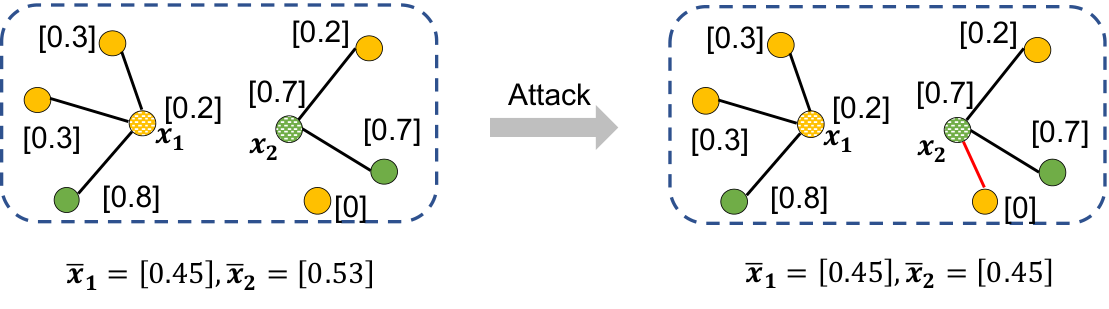
Remark 1. Note that the existence of two nodes with the same aggregated features but different labels is not rare when considering adversarial attack or abnormal features. We provide a figurative example in Figure 5 in Appendix A.3: the attacker injects one adversarial edge into the graph and changes the aggregated features and to be the same.
Remark 2. When we consider , whether we can find satisfying and depends on the expressiveness of the the transformation function. If it is not powerful enough (e.g., an under-parameterized neural network), it could fail to map different data points to different labels. On the contrary, adapting the data does not suffer this problem as we can always modify the test graph to satisfy and .
Remark 3. The above discussion can be easily extended to nonlinear GNN by considering as the output before the last linear layer of GNN.
4 Experiment
4.1 Generalization on Out-of-distribution Data
Setup. Following the settings in EERM (Wu et al. 2022a), which is designed for node-level tasks on OOD data, we validate GTrans on three types of distribution shifts with six benchmark datasets: (1) artificial transformation for Cora (Yang et al. 2016) and Amazon-Photo (Shchur et al. 2018), (2) cross-domain transfers for Twitch-E and FB-100 (Rozemberczki et al. 2021a) (Lim et al. 2021), and (3) temporal evolution for Elliptic (Pareja et al. 2020) and OGB-Arxiv (Hu et al. 2020). Moreoever, Cora and Amazon-Photo have 1/1/8 graphs for training/validation/test sets. The splits are 1/1/5 on Twitch-E, 3/2/3 on FB-100, 5/5/33 on Elliptic, and 1/1/3 on OGB-Arxiv. More details on the datasets are provided in Appendix C. We compare GTrans with four baselines: empirical risk minimization (ERM, i.e., standard training), data augmentation technique DropEdge (Rong et al. 2020), test-time-training method Tent (Wang et al. 2021), and the recent SOTA method EERM (Wu et al. 2022a) which is exclusively developed for graph OOD issue. Further, we evaluate all the methods with four popular GNN backbones including GCN (Kipf & Welling 2016a), GraphSAGE (Hamilton et al. 2017), GAT (Veličković et al. 2018), and GPR (Chien et al. 2021). Their default setup follows that in EERM22 2 We note that the GCN used in the experiments of EERM does not normalize the adjacency matrix according to its open-source code. Here we normalize the adjacency matrix to make it consistent with the original GCN.. We refer the readers to Appendix 5 for more implementation details of baselines and GTrans. Notably, all experiments in this paper are repeated 10 times with different random seeds. Due to page limit, we include more baselines such as SR-GNN (Zhu et al. 2021a) and UDA-GCN (Wu et al. 2020) in Appendix D.1.
Results. Table 1 reports the averaged performance over the test graphs for each dataset as well as the averaged rank of each algorithm. From the table, we make the following observations:
(a) Overall Performance. The proposed framework consistently achieves strong performance across the datasets: GTrans achieves average ranks of 1.0, 1.7, 2.0 and 1.7 with GCN, SAGE, GAT and GPR, respectively, while the corresponding ranks for the best baseline EERM are 2.9, 3.4, 3.0 and 2.0. Furthermore, in most of the cases, GTrans significantly improves the vanilla baseline (ERM) by a large margin. Particularly, when using GCN as backbone, GTrans outperforms ERM by 3.1%, 5.0% and 2.0% on Cora, Elliptic and OGB-Arxiv, respectively. These results demonstrate the effectiveness of GTrans in tackling diverse types of distribution shifts.
(b) Comparison to other baselines. Both DropEdge and EERM modify the training process to improve model generalization. Nonetheless, they are less effective than GTrans, as GTrans takes advantage of the information from test graphs. As a test-time training method, Tent also performs well in some cases, but Tent only adapts the parameters in batch normalization layers and cannot be applied to models without batch normalization.
We further show the performance on each test graph on Cora with GCN in Figure 2 and the results for other datasets are provided in Appendix D.4. We observe that GTrans generally improves over individual test graphs within each dataset, which validates the effectiveness of GTrans.
Efficiency Comparison. Since EERM performs the best among baselines, Table 2 showcases the efficiency comparison between our proposed GTrans and EERM on the largest test graph in each dataset. The additional running time of GTrans majorly depends on the number of gradient descent steps. As we only use a small number (5 or 10) throughout all the experiments, the time overhead brought by GTrans is negligible. Compared with the re-training method EERM, GTrans avoids the complex bilevel optimization and thus is significantly more efficient. Furthermore, EERM imposes a considerably heavier memory burden.
| Backbone | Method | Amz-Photo | Cora | Elliptic | FB-100 | OGB-Arxiv | Twitch-E | Rank |
|---|---|---|---|---|---|---|---|---|
| GCN | ERM | 93.79±0.97 | 91.59±1.44 | 50.90±1.51 | 54.04±0.94 | 38.59±1.35 | 59.89±0.50 | 3.8 |
| DropEdge | 92.11±0.31 | 81.01±1.33 | 53.96±4.91 | 53.00±0.50 | 41.26±0.92 | 59.95±0.39 | 3.6 | |
| Tent | 94.03±1.07 | 91.87±1.36 | 51.71±2.00 | 54.16±1.00 | 39.33±1.40 | 59.46±0.55 | 3.3 | |
| EERM | 94.05±0.40 | 87.21±0.53 | 53.96±0.65 | 54.24±0.55 | OOM | 59.85±0.85 | 2.9 | |
| GTrans | 94.13±0.77∗ | 94.66±0.63∗∗ | 55.88±3.10∗∗ | 54.32±0.60 | 41.59±1.20∗∗ | 60.42±0.86∗ | 1.0 | |
| SAGE | ERM | 95.09±0.60 | 99.67±0.14 | 56.12±4.47 | 54.70±0.47 | 39.56±1.66 | 62.06±0.09 | 3.2 |
| DropEdge | 92.61±0.56 | 95.85±0.30 | 52.38±3.11 | 54.51±0.69 | 38.89±1.74 | 62.14±0.12 | 4.2 | |
| Tent | 95.72±0.43 | 99.80±0.10 | 55.89±4.87 | 54.86±0.34 | 39.58±1.26 | 62.09±0.09 | 2.3 | |
| EERM | 95.57±0.13 | 98.77±0.14 | 58.20±3.55 | 54.28±0.97 | OOM | 62.11±0.12 | 3.4 | |
| GTrans | 96.91±0.68∗∗ | 99.45±0.13 | 60.81±5.19∗∗ | 54.64±0.62 | 40.39±1.45∗∗ | 62.15±0.13∗ | 1.7 | |
| GAT | ERM | 96.30±0.79 | 94.81±1.28 | 65.36±2.70 | 51.77±1.41 | 40.63±1.57 | 58.53±1.00 | 3.0 |
| DropEdge | 90.70±0.29 | 76.91±1.55 | 63.78±2.39 | 52.65±0.88 | 42.48±0.93 | 58.89±1.01 | 3.3 | |
| Tent | 95.99±0.46 | 95.91±1.14 | 66.07±1.66 | 51.47±1.70 | 40.06±1.19 | 58.33±1.18 | 3.3 | |
| EERM | 95.57±1.32 | 85.00±0.96 | 58.14±4.71 | 53.30±0.77 | OOM | 59.84±0.71 | 3.0 | |
| GTrans | 96.67±0.74∗∗ | 96.37±1.00∗∗ | 66.43±2.57∗∗ | 51.16±1.72 | 43.76±1.25∗∗ | 58.59±1.07 | 2.0 | |
| GPR | ERM | 91.87±0.65 | 93.00±2.17 | 64.59±3.52 | 54.51±0.33 | 44.38±0.59 | 59.72±0.40 | 2.7 |
| DropEdge | 88.81±1.48 | 79.27±1.39 | 61.02±1.78 | 55.04±0.33 | 43.65±0.77 | 59.89±0.05 | 3.3 | |
| Tent33 3 | - | - | - | - | - | - | - | |
| EERM | 90.78±0.52 | 88.82±3.10 | 67.27±0.98 | 55.95±0.03 | OOM | 61.57±0.12 | 2.0 | |
| GTrans | 91.93±0.73 | 93.05±2.02 | 69.03±2.33∗∗ | 54.38±0.31 | 46.00±0.46∗∗ | 60.11±0.53∗∗ | 1.7 |
- 3
Tent cannot be applied to models which do not contain batch normalization layers.
figureResults on Cora under OOD. GTrans improves GCN on most test graphs.
| Extra Running Time (s) | Total GPU Memory (GB) | |||||||
| Cora | Photo | Ellip. | Arxiv | Cora | Photo | Ellip. | Arxiv | |
| EERM | 25.9 | 396.4 | 607.9 | - | 2.5 | 10.5 | 12.8 | 32 |
| GTrans | 0.3 | 0.5 | 0.6 | 2.6 | 1.4 | 1.5 | 1.3 | 3.9 |
4.2 Robustness to Abnormal Features
Setup. Following the setup in AirGNN (Liu et al. 2021a), we evaluate the robustness in the case of abnormal features. Specifically, we simulate abnormal features by assigning random features taken from a multivariate standard Gaussian distribution to a portion of randomly selected test nodes. Note that the abnormal features are injected after model training (at test time) and we vary the ratio of noisy nodes from 0.1 to 0.4 with a step size of 0.05. This process is performed for four datasets: the original version of Cora, Citeseer, Pubmed, and OGB-Arxiv. In these four datasets, the training graph and the test graph have the same graph structure but the node features are different. Hence, we use the training classification loss combined with the proposed contrastive loss to optimize GTrans. We use GCN as the backbone model and adopt four GNNs as the baselines including GAT (Veličković et al. 2018), APPNP (Klicpera et al. 2018), AirGNN and AirGNN-t. Note that AirGNN-t tunes the message-passing hyper-parameter in AirGNN at test time. For a fair comparison, we tune AirGNN-t based on the performance on both training and validation nodes.
Results. For each model, we present the node classification accuracy on both abnormal nodes and all test nodes (i.e., both normal and abnormal ones) in Figure 3 and Figure 7 (See Appendix D.5), respectively. From these figures, we have two observations. First, GTrans significantly improves GCN in terms of the performance on abnormal nodes and all test nodes for all datasets across all noise ratios. For example, on Cora with 30% noisy nodes, GTrans improves GCN by 48.2% on abnormal nodes and 31.0% on overall test accuracy. This demonstrates the effectiveness of the graph transformation process in GTrans in alleviating the effect of abnormal features. Second, GTrans shows comparable or better performance with AirGNNs, which are the SOTA defense methods for tackling abnormal features. It is worth mentioning that AirGNN-t improves AirGNN by tuning its hyper-parameter at test time, which aligns with our motivation that test-time adaptation can enhance model test performance. To further understand the effect of graph transformation, we provide the visualization of the test node embeddings obtained from abnormal graph (0.3 noise ratio) and transformed graph for Cora in Figures 4a and 4b, respectively. We observe that the transformed graph results in well-clustered node representations, which indicates that GTrans can promote intra-class compactness and counteract the effect of abnormal patterns.

4.3 Robustness to Adversarial Attack
Setup. We further evaluate GTrans under the setting of adversarial attack where we perturb the test graph, i.e., evasion attack. Specifically, we use PR-BCD (Geisler et al. 2021), a scalable attack method, to attack the test graph in OGB-Arxiv. We focus on structural attacks, and vary the perturbation rate, i.e., the ratio of changed edges, from 5% to 25% with a step of 5%. Similar to Section 4.2, we adopt the training classification loss together with the proposed contrastive loss to optimize GTrans. We use GCN as the backbone and employ four robust baselines implemented by the adversarial attack repository DeepRobust (Li et al. 2020) including GAT (Veličković et al. 2018), RobustGCN (Zhu et al. 2019), SimPGCN (Jin et al. 2021a) and GCNJaccard (Xu et al. 2019) as comparisons. Among them, GCNJaccard pre-processes the attacked graph by removing edges where the similarities of connected nodes are less than a threshold; we tune this threshold at test time based on the performance on both training and validation nodes.
Results. Table 3 reports the performances under structural evasion attack. We observe that GTrans consistently improves the performance of GCN under different perturbation rates of adversarial attack. Particularly, GTrans improves GCN by a larger margin when the perturbation rate is higher. For example, GTrans outperforms GCN by over 40% under the 25% perturbation rate. Such observation suggests that GTrans can counteract the devastating effect of adversarial attacks. In addition, the best performing baseline GCNJaccard also modifies the graph at test time, which demonstrates the importance of test-time graph adaptation. Nonetheless, it consistently underperforms our proposed GTrans, indicating that a learnable transformation function is needed to achieve better robustness under adversarial attacks, which GCNJaccard does not employ.
Interpretation. To understand the modifications made on the graph, we compare several properties among clean graph, attacked graph (20% perturbation rate), graph obtained by GCNJaccard, and graph obtained by GTrans in Table 13 in Appendix D.6. First, adversarial attack decreases homophily and feature similarity, but GTrans and GCNJaccard promote such information to alleivate the adversarial patterns. Our experiment also shows that GTrans removes 77% adversarial edges while removing 30% existing edges from the attacked graph. Second, both GTrans and GCNJaccard focus on deleting edges from the attacked graph, but GCNJaccard removes a substantially larger amount of edges, which may destroy clean graph structure and lead to sub-optimal performance.
| Ptb. Rate | GCN | GAT | RobustGCN | SimPGCN | GCNJaccard | GTrans |
|---|---|---|---|---|---|---|
| 5% | 57.47±0.54 | 64.56±0.43 | 61.55±1.20 | 61.30±0.42 | 65.01±0.26 | 66.29±0.25 |
| 10% | 47.97±0.65 | 61.20±0.70 | 58.15±1.55 | 57.01±0.70 | 63.25±0.30 | 65.16±0.52 |
| 15% | 38.04±1.22 | 58.96±0.59 | 55.91±1.27 | 54.13±0.73 | 61.83±0.29 | 64.40±0.38 |
| 20% | 29.05±0.73 | 57.29±0.49 | 54.39±1.09 | 52.26±0.87 | 60.57±0.34 | 63.44±0.50 |
| 25% | 19.58±2.32 | 55.86±0.53 | 52.76±1.44 | 50.46±0.85 | 59.17±0.39 | 62.95±0.67 |
| Tr\Te | GCN | APPNP | AirGNN | GAT |
|---|---|---|---|---|
| GCN | 67.36 | 70.65 | 70.84 | 58.62 |
| APPNP | 67.87 | 70.39 | 69.59 | 64.46 |
| AirGNN | 68.00 | 70.37 | 72.68 | 64.93 |
| GAT | 54.85 | 60.37 | 65.22 | 54.60 |
| Noisy | 44.29 | 48.26 | 58.51 | 21.23 |
4.4 Further Analysis
Cross-Architecture Transferability. Since the outcome of GTrans is a refined graph, it can conceptually be employed by any GNN model. Thus, we can transform the graph based on one pre-trained GNN and test the transformed graph on another pre-trained GNN. To examine such transferability, we perform experiments GCN, APPNP, AirGNN and GAT under the abnormal feature setting with 30% noisy nodes on Cora. The results on all test nodes in Table 4.3. Note that “Tr” stands for GNNs used in TTGT while “Te” denotes GNNs used for obtaining predictions on the transformed graph; “Noisy” indicates the performance on the noisy graph. We observe that the transformed graph yields good performance even outside the scope it was optimized for. We anticipate that such transferability can alleviate the need for costly re-training on new GNNs.
Adapting Model vs. Adapting Data. We empirically compare the performance between adapting data and adapting model and consider the OOD and abnormal feature settings. Specifically, we use GCN as the backbone and adapt the model parameters by optimizing the same loss function as used in GTrans. The results are shown in Figures 4c and 4d. In OOD setting, both adapting model and adapting data can generally improve GCN’s performance. Since their performances are still close, it is hard to give a definite answer on which strategy is better. However, we can observe significant performance differences when the graph contains abnormal features: adapting data outperforms adapting model on 3 out of 4 datasets. This suggests that adapting data can be more powerful when the data is perturbed, which aligns with our analysis in Section 3.3.
Learning Features v.s. Learning Structure. Since our framework learns both node features and graph structure, we investigate when one component plays a more important role than the other. Our results are shown in Tables 16 and 17 in Appendix D.8. From the tables, we observe that (1) while each component can improve the vanilla performance, feature learning is more crucial for counteracting feature corruption and structure learning is more important for defending structure corruption; and (2) combining them generally yields a better or comparable performance.
5 Conclusion
GNNs tend to yield unsatisfying performance when the presented data is sub-optimal. To tackle this issue, we seek to enhance GNNs from a data-centric perspective by transforming the graph data at test time. We propose GTrans which optimizes a contrastive surrogate loss to transform graph structure and node features, and provide theoretical analysis with deeper discussion to understand this framework. Experimental results on distribution shift, abnormal features and adversarial attack have demonstrated the effectiveness of our method. In the future, we plan to explore more applications of our framework such as mitigating degree bias and long-range dependency.
Acknolwedgement
This research is supported by the National Science Foundation (NSF) under grant numbers IIS1845081, IIS1928278, IIS1955285, IIS2212032, IIS2212144, IOS2107215, and IOS2035472, the Army Research Office (ARO) under grant number W911NF-21-1-0198, MSU Foundation, the Home Depot, Cisco Systems Inc, Amazon Faculty Award, Johnson & Johnson and Snap Inc.
Ethics Statement
To the best of our knowledge, there are no ethical issues with this paper.
Reproducibility Statement
To ensure reproducibility of our experiments, we provide our source code at https://github.com/ChandlerBang/GTrans. The hyper-parameters are described in details in the appendix. We also provide a pseudo-code implementation of our framework in the appendix.
References
- Boudiaf et al. (2020) Malik Boudiaf, Jérôme Rony, Imtiaz Masud Ziko, Eric Granger, Marco Pedersoli, Pablo Piantanida, and Ismail Ben Ayed. A unifying mutual information view of metric learning: cross-entropy vs. pairwise losses. In European conference on computer vision, pp. 548–564. Springer, 2020.
- Buffelli et al. (2022) Davide Buffelli, Pietro Liò, and Fabio Vandin. Sizeshiftreg: a regularization method for improving size-generalization in graph neural networks. Advances in Neural Information Processing Systems, 2022.
- Chen et al. (2022) Yongqiang Chen, Yonggang Zhang, Han Yang, Kaili Ma, Binghui Xie, Tongliang Liu, Bo Han, and James Cheng. Invariance principle meets out-of-distribution generalization on graphs. arXiv preprint arXiv:2202.05441, 2022.
- Chen et al. (2020) Yu Chen, Lingfei Wu, and Mohammed Zaki. Iterative deep graph learning for graph neural networks: Better and robust node embeddings. In H. Larochelle, M. Ranzato, R. Hadsell, M.F. Balcan, and H. Lin (eds.), Advances in Neural Information Processing Systems, volume 33, pp. 19314–19326, 2020.
- Chien et al. (2021) Eli Chien, Jianhao Peng, Pan Li, and Olgica Milenkovic. Adaptive universal generalized pagerank graph neural network. In ICLR, 2021. URL https://openreview.net/forum?id=n6jl7fLxrP.
- Deng & Hooi (2021) Ailin Deng and Bryan Hooi. Graph neural network-based anomaly detection in multivariate time series. In Proceedings of the AAAI Conference on Artificial Intelligence, volume 35, pp. 4027–4035, 2021.
- Derrow-Pinion et al. (2021) Austin Derrow-Pinion, Jennifer She, David Wong, Oliver Lange, Todd Hester, Luis Perez, Marc Nunkesser, Seongjae Lee, Xueying Guo, Brett Wiltshire, et al. Eta prediction with graph neural networks in google maps. In Proceedings of the 30th ACM International Conference on Information & Knowledge Management, pp. 3767–3776, 2021.
- Ding et al. (2022) Kaize Ding, Zhe Xu, Hanghang Tong, and Huan Liu. Data augmentation for deep graph learning: A survey. arXiv preprint arXiv:2202.08235, 2022.
- Duvenaud et al. (2015) David K Duvenaud, Dougal Maclaurin, Jorge Iparraguirre, Rafael Bombarell, Timothy Hirzel, Alán Aspuru-Guzik, and Ryan P Adams. Convolutional networks on graphs for learning molecular fingerprints. Advances in neural information processing systems, 28, 2015.
- Entezari et al. (2020) Negin Entezari, Saba A Al-Sayouri, Amirali Darvishzadeh, and Evangelos E Papalexakis. All you need is low (rank) defending against adversarial attacks on graphs. In Proceedings of the 13th International Conference on Web Search and Data Mining, pp. 169–177, 2020.
- Fan et al. (2019) Wenqi Fan, Yao Ma, Qing Li, Yuan He, Eric Zhao, Jiliang Tang, and Dawei Yin. Graph neural networks for social recommendation. In The world wide web conference, pp. 417–426, 2019.
- Fatemi et al. (2021) Bahare Fatemi, Layla El Asri, and Seyed Mehran Kazemi. Slaps: Self-supervision improves structure learning for graph neural networks. Advances in Neural Information Processing Systems, 34:22667–22681, 2021.
- Feng et al. (2020) Wenzheng Feng, Jie Zhang, Yuxiao Dong, Yu Han, Huanbo Luan, Qian Xu, Qiang Yang, Evgeny Kharlamov, and Jie Tang. Graph random neural networks for semi-supervised learning on graphs. Advances in neural information processing systems, 33:22092–22103, 2020.
- Franceschi et al. (2019) Luca Franceschi, Mathias Niepert, Massimiliano Pontil, and Xiao He. Learning discrete structures for graph neural networks. arXiv preprint arXiv:1903.11960, 2019.
- Ganin et al. (2016) Yaroslav Ganin, Evgeniya Ustinova, Hana Ajakan, Pascal Germain, Hugo Larochelle, François Laviolette, Mario Marchand, and Victor Lempitsky. Domain-adversarial training of neural networks. The journal of machine learning research, 17(1):2096–2030, 2016.
- Geisler et al. (2021) Simon Geisler, Tobias Schmidt, Hakan Şirin, Daniel Zügner, Aleksandar Bojchevski, and Stephan Günnemann. Robustness of graph neural networks at scale. Advances in Neural Information Processing Systems, 34:7637–7649, 2021.
- Gui et al. (2022) Shurui Gui, Xiner Li, Limei Wang, and Shuiwang Ji. Good: A graph out-of-distribution benchmark. arXiv preprint arXiv:2206.08452, 2022.
- Guo et al. (2022) Zhichun Guo, Bozhao Nan, Yijun Tian, Olaf Wiest, Chuxu Zhang, and Nitesh V Chawla. Graph-based molecular representation learning. arXiv preprint arXiv:2207.04869, 2022.
- Halcrow et al. (2020) Jonathan Halcrow, Alexandru Mosoi, Sam Ruth, and Bryan Perozzi. Grale: Designing networks for graph learning. In Proceedings of the 26th ACM SIGKDD International Conference on Knowledge Discovery & Data Mining, pp. 2523–2532, 2020.
- Hamilton et al. (2017) Will Hamilton, Zhitao Ying, and Jure Leskovec. Inductive representation learning on large graphs. Advances in neural information processing systems, 30, 2017.
- Hassani & Khasahmadi (2020) Kaveh Hassani and Amir Hosein Khasahmadi. Contrastive multi-view representation learning on graphs. In International Conference on Machine Learning, pp. 4116–4126. PMLR, 2020.
- Hu et al. (2020) Weihua Hu, Matthias Fey, Marinka Zitnik, Yuxiao Dong, Hongyu Ren, Bowen Liu, Michele Catasta, and Jure Leskovec. Open graph benchmark: Datasets for machine learning on graphs. Advances in neural information processing systems, 33:22118–22133, 2020.
- Jin et al. (2020) Wei Jin, Yao Ma, Xiaorui Liu, Xianfeng Tang, Suhang Wang, and Jiliang Tang. Graph structure learning for robust graph neural networks. arXiv preprint arXiv:2005.10203, 2020.
- Jin et al. (2021a) Wei Jin, Tyler Derr, Yiqi Wang, Yao Ma, Zitao Liu, and Jiliang Tang. Node similarity preserving graph convolutional networks. In Proceedings of the 14th ACM international conference on web search and data mining, pp. 148–156, 2021a.
- Jin et al. (2021b) Wei Jin, Yaxing Li, Han Xu, Yiqi Wang, Shuiwang Ji, Charu Aggarwal, and Jiliang Tang. Adversarial attacks and defenses on graphs. ACM SIGKDD Explorations Newsletter, 22(2):19–34, 2021b.
- Kipf & Welling (2016a) Thomas N Kipf and Max Welling. Semi-supervised classification with graph convolutional networks. arXiv preprint arXiv:1609.02907, 2016a.
- Kipf & Welling (2016b) Thomas N Kipf and Max Welling. Variational graph auto-encoders. arXiv preprint arXiv:1611.07308, 2016b.
- Klicpera et al. (2018) Johannes Klicpera, Aleksandar Bojchevski, and Stephan Günnemann. Predict then propagate: Graph neural networks meet personalized pagerank. arXiv preprint arXiv:1810.05997, 2018.
- Li et al. (2022) Haoyang Li, Xin Wang, Ziwei Zhang, and Wenwu Zhu. Out-of-distribution generalization on graphs: A survey. arXiv preprint arXiv:2202.07987, 2022.
- Li et al. (2021) Jintang Li, Tao Xie, Chen Liang, Fenfang Xie, Xiangnan He, and Zibin Zheng. Adversarial attack on large scale graph. IEEE Transactions on Knowledge and Data Engineering, 2021.
- Li et al. (2020) Yaxin Li, Wei Jin, Han Xu, and Jiliang Tang. Deeprobust: A pytorch library for adversarial attacks and defenses. arXiv preprint arXiv:2005.06149, 2020.
- Lim et al. (2021) Derek Lim, Xiuyu Li, Felix Hohne, and Ser-Nam Lim. New benchmarks for learning on non-homophilous graphs. arXiv preprint arXiv:2104.01404, 2021.
- Liu et al. (2022a) Hongrui Liu, Binbin Hu, Xiao Wang, Chuan Shi, Zhiqiang Zhang, and Jun Zhou. Confidence may cheat: Self-training on graph neural networks under distribution shift. In Proceedings of the ACM Web Conference 2022, pp. 1248–1258, 2022a.
- Liu et al. (2015) Sijia Liu, Swarnendu Kar, Makan Fardad, and Pramod K Varshney. Sparsity-aware sensor collaboration for linear coherent estimation. IEEE Transactions on Signal Processing, 63(10):2582–2596, 2015.
- Liu et al. (2021a) Xiaorui Liu, Jiayuan Ding, Wei Jin, Han Xu, Yao Ma, Zitao Liu, and Jiliang Tang. Graph neural networks with adaptive residual. In A. Beygelzimer, Y. Dauphin, P. Liang, and J. Wortman Vaughan (eds.), Advances in Neural Information Processing Systems, 2021a. URL https://openreview.net/forum?id=hfkER_KJiNw.
- Liu et al. (2022b) Yixin Liu, Ming Jin, Shirui Pan, Chuan Zhou, Yu Zheng, Feng Xia, and Philip Yu. Graph self-supervised learning: A survey. IEEE Transactions on Knowledge and Data Engineering, 2022b.
- Liu et al. (2021b) Yuejiang Liu, Parth Kothari, Bastien van Delft, Baptiste Bellot-Gurlet, Taylor Mordan, and Alexandre Alahi. Ttt++: When does self-supervised test-time training fail or thrive? Advances in Neural Information Processing Systems, 34:21808–21820, 2021b.
- Pareja et al. (2020) Aldo Pareja, Giacomo Domeniconi, Jie Chen, Tengfei Ma, Toyotaro Suzumura, Hiroki Kanezashi, Tim Kaler, Tao Schardl, and Charles Leiserson. Evolvegcn: Evolving graph convolutional networks for dynamic graphs. In Proceedings of the AAAI Conference on Artificial Intelligence, volume 34, pp. 5363–5370, 2020.
- Rong et al. (2020) Yu Rong, Wenbing Huang, Tingyang Xu, and Junzhou Huang. Dropedge: Towards deep graph convolutional networks on node classification. In International Conference on Learning Representations, 2020. URL https://openreview.net/forum?id=Hkx1qkrKPr.
- Rozemberczki et al. (2021a) Benedek Rozemberczki, Carl Allen, and Rik Sarkar. Multi-scale attributed node embedding. Journal of Complex Networks, 9(2):cnab014, 2021a.
- Rozemberczki et al. (2021b) Benedek Rozemberczki, Peter Englert, Amol Kapoor, Martin Blais, and Bryan Perozzi. Pathfinder discovery networks for neural message passing. In Proceedings of the Web Conference 2021, pp. 2547–2558, 2021b.
- Sankar et al. (2021) Aravind Sankar, Yozen Liu, Jun Yu, and Neil Shah. Graph neural networks for friend ranking in large-scale social platforms. In Proceedings of the Web Conference 2021, pp. 2535–2546, 2021.
- Shchur et al. (2018) Oleksandr Shchur, Maximilian Mumme, Aleksandar Bojchevski, and Stephan Günnemann. Pitfalls of graph neural network evaluation. arXiv preprint arXiv:1811.05868, 2018.
- Shen et al. (2020) Xiao Shen, Quanyu Dai, Fu-lai Chung, Wei Lu, and Kup-Sze Choi. Adversarial deep network embedding for cross-network node classification. In Proceedings of the AAAI Conference on Artificial Intelligence, volume 34, pp. 2991–2999, 2020.
- Sun et al. (2020) Yu Sun, Xiaolong Wang, Zhuang Liu, John Miller, Alexei Efros, and Moritz Hardt. Test-time training with self-supervision for generalization under distribution shifts. In International conference on machine learning, pp. 9229–9248. PMLR, 2020.
- Suresh et al. (2021) Susheel Suresh, Pan Li, Cong Hao, and Jennifer Neville. Adversarial graph augmentation to improve graph contrastive learning. Advances in Neural Information Processing Systems, 34:15920–15933, 2021.
- Tang et al. (2020) Xianfeng Tang, Yozen Liu, Neil Shah, Xiaolin Shi, Prasenjit Mitra, and Suhang Wang. Knowing your fate: Friendship, action and temporal explanations for user engagement prediction on social apps. In Proceedings of the 26th ACM SIGKDD international conference on knowledge discovery & data mining, pp. 2269–2279, 2020.
- Traud et al. (2012) Amanda L Traud, Peter J Mucha, and Mason A Porter. Social structure of facebook networks. Physica A: Statistical Mechanics and its Applications, 391(16):4165–4180, 2012.
- Veličković et al. (2018) Petar Veličković, Guillem Cucurull, Arantxa Casanova, Adriana Romero, Pietro Lio, and Yoshua Bengio. Graph attention networks. 2018.
- Velickovic et al. (2019) Petar Velickovic, William Fedus, William L Hamilton, Pietro Liò, Yoshua Bengio, and R Devon Hjelm. Deep graph infomax. ICLR (Poster), 2(3):4, 2019.
- Wang et al. (2021) Dequan Wang, Evan Shelhamer, Shaoteng Liu, Bruno Olshausen, and Trevor Darrell. Tent: Fully test-time adaptation by entropy minimization. In International Conference on Learning Representations, 2021. URL https://openreview.net/forum?id=uXl3bZLkr3c.
- Wu et al. (2020) Man Wu, Shirui Pan, Chuan Zhou, Xiaojun Chang, and Xingquan Zhu. Unsupervised domain adaptive graph convolutional networks. In Proceedings of The Web Conference 2020, pp. 1457–1467, 2020.
- Wu et al. (2022a) Qitian Wu, Hengrui Zhang, Junchi Yan, and David Wipf. Handling distribution shifts on graphs: An invariance perspective. In International Conference on Learning Representations, 2022a. URL https://openreview.net/forum?id=FQOC5u-1egI.
- Wu et al. (2022b) Yingxin Wu, Xiang Wang, An Zhang, Xiangnan He, and Tat-Seng Chua. Discovering invariant rationales for graph neural networks. In International Conference on Learning Representations, 2022b. URL https://openreview.net/forum?id=hGXij5rfiHw.
- Wu et al. (2019) Zonghan Wu, Shirui Pan, Fengwen Chen, Guodong Long, Chengqi Zhang, and Philip S Yu. A comprehensive survey on graph neural networks. arXiv preprint arXiv:1901.00596, 2019.
- Xie et al. (2021) Yaochen Xie, Zhao Xu, Jingtun Zhang, Zhengyang Wang, and Shuiwang Ji. Self-supervised learning of graph neural networks: A unified review. arXiv preprint arXiv:2102.10757, 2021.
- Xu et al. (2019) Kaidi Xu, Hongge Chen, Sijia Liu, Pin-Yu Chen, Tsui-Wei Weng, Mingyi Hong, and Xue Lin. Topology attack and defense for graph neural networks: An optimization perspective. arXiv preprint arXiv:1906.04214, 2019.
- Yang et al. (2021a) Jingkang Yang, Kaiyang Zhou, Yixuan Li, and Ziwei Liu. Generalized out-of-distribution detection: A survey. arXiv preprint arXiv:2110.11334, 2021a.
- Yang et al. (2021b) Shuo Yang, Lu Liu, and Min Xu. Free lunch for few-shot learning: Distribution calibration. In International Conference on Learning Representations (ICLR), 2021b.
- Yang et al. (2021c) Shuo Yang, Songhua Wu, Tongliang Liu, and Min Xu. Bridging the gap between few-shot and many-shot learning via distribution calibration. IEEE Transactions on Pattern Analysis and Machine Intelligence, 44(12):9830–9843, 2021c.
- Yang et al. (2016) Zhilin Yang, William Cohen, and Ruslan Salakhudinov. Revisiting semi-supervised learning with graph embeddings. In International conference on machine learning, pp. 40–48. PMLR, 2016.
- Ying et al. (2018) Rex Ying, Ruining He, Kaifeng Chen, Pong Eksombatchai, William L Hamilton, and Jure Leskovec. Graph convolutional neural networks for web-scale recommender systems. In Proceedings of the 24th ACM SIGKDD international conference on knowledge discovery & data mining, pp. 974–983, 2018.
- You et al. (2020) Yuning You, Tianlong Chen, Yongduo Sui, Ting Chen, Zhangyang Wang, and Yang Shen. Graph contrastive learning with augmentations. Advances in Neural Information Processing Systems, 33:5812–5823, 2020.
- You et al. (2021) Yuning You, Tianlong Chen, Yang Shen, and Zhangyang Wang. Graph contrastive learning automated. Proceedings of International Conference on Machine Learning, 2021.
- You et al. (2023) Yuning You, Tianlong Chen, Zhangyang Wang, and Yang Shen. Graph domain adaptation via theory-grounded spectral regularization. In International Conference on Learning Representations, 2023.
- Zellinger et al. (2017) Werner Zellinger, Thomas Grubinger, Edwin Lughofer, Thomas Natschläger, and Susanne Saminger-Platz. Central moment discrepancy (cmd) for domain-invariant representation learning. arXiv preprint arXiv:1702.08811, 2017.
- Zhang et al. (2021) Marvin Zhang, Sergey Levine, and Chelsea Finn. Memo: Test time robustness via adaptation and augmentation. arXiv preprint arXiv:2110.09506, 2021.
- Zhang et al. (2022) Yifan Zhang, Bryan Hooi, Lanqing Hong, and Jiashi Feng. Self-supervised aggregation of diverse experts for test-agnostic long-tailed recognition. In Advances in Neural Information Processing Systems, 2022.
- Zhao et al. (2021a) Tong Zhao, Tianwen Jiang, Neil Shah, and Meng Jiang. A synergistic approach for graph anomaly detection with pattern mining and feature learning. IEEE Transactions on Neural Networks and Learning Systems, 2021a.
- Zhao et al. (2021b) Tong Zhao, Yozen Liu, Leonardo Neves, Oliver Woodford, Meng Jiang, and Neil Shah. Data augmentation for graph neural networks. In AAAI, 2021b.
- Zhao et al. (2022a) Tong Zhao, Wei Jin, Yozen Liu, Yingheng Wang, Gang Liu, Stephan Günneman, Neil Shah, and Meng Jiang. Graph data augmentation for graph machine learning: A survey. arXiv preprint arXiv:2202.08871, 2022a.
- Zhao et al. (2022b) Tong Zhao, Gang Liu, Daheng Wang, Wenhao Yu, and Meng Jiang. Learning from counterfactual links for link prediction. In International Conference on Machine Learning, pp. 26911–26926. PMLR, 2022b.
- Zhu et al. (2019) Dingyuan Zhu, Ziwei Zhang, Peng Cui, and Wenwu Zhu. Robust graph convolutional networks against adversarial attacks. In Proceedings of the 25th ACM SIGKDD international conference on knowledge discovery & data mining, pp. 1399–1407, 2019.
- Zhu et al. (2020) Jiong Zhu, Yujun Yan, Lingxiao Zhao, Mark Heimann, Leman Akoglu, and Danai Koutra. Beyond homophily in graph neural networks: Current limitations and effective designs. Advances in Neural Information Processing Systems, 33:7793–7804, 2020.
- Zhu et al. (2021a) Qi Zhu, Natalia Ponomareva, Jiawei Han, and Bryan Perozzi. Shift-robust gnns: Overcoming the limitations of localized graph training data. Advances in Neural Information Processing Systems, 34, 2021a.
- Zhu et al. (2021b) Yanqiao Zhu, Yichen Xu, Feng Yu, Qiang Liu, Shu Wu, and Liang Wang. Graph contrastive learning with adaptive augmentation. In Proceedings of the Web Conference 2021, pp. 2069–2080, 2021b.
- Zügner et al. (2018) Daniel Zügner, Amir Akbarnejad, and Stephan Günnemann. Adversarial attacks on neural networks for graph data. In Proceedings of the 24th ACM SIGKDD international conference on knowledge discovery & data mining, pp. 2847–2856, 2018.
- Zügner & Günnemann (2019) Daniel Zügner and Stephan Günnemann. Adversarial attacks on graph neural networks via meta learning. In International Conference on Learning Representations, 2019. URL https://openreview.net/forum?id=Bylnx209YX.
Appendix A Proofs
A.1 Thereom 1
Theorem 1.
Let denote the classification loss and denote the surrogate loss, respectively. Let denote the correlation between and , and let denote the learning rate for gradient descent. Assume that is twice-differentiable and its Hessian matrix satisfies for all . When and , we have
| (8) |
Proof.
Given that is differentiable and twice-differentiable, we perform first-order Taylor expansion with Lagrange form of remainder at :
| (9) | ||||
where is a constant given by Lagrange form of the Taylor’s remainder (here we slightly abuse the notation), and is the correlation between and :
| (10) |
Before we proceed to the next steps, we first show that given a vector and a symmetric matrix , the inequality holds:
| (11) |
Since the Hessian matrix is symmetric, we can use the above inequality to derive:
| (12) | ||||
Then we rewrite Eq. (12) as:
| (13) | ||||
Given , we know
| (14) | ||||
By setting , we have
| (15) |
Therefore, when and , we have
| (16) |
∎
A.2 Thereom 2
Theorem 2.
Assume that the augmentation function generates a data view of the same class for the test nodes and the node classes are balanced. Assume for each class, the mean of the representations obtained from and are the same. Minimizing the first term in Eq. (6) is approximately minimizing the class-conditional entropy between features and labels .
Proof.
For convenience, we slightly abuse the notations to replace and with and , respectively. Then we have . Let denote the set of test samples from class ; thus . Let denote equality up to a multiplicative and/or additive constant. Then the first term in Eq. (6) can be rewritten as:
| (17) |
Let be the mean of hidden representations from class ; then we have . Now we build the connection between Eq. (17) and :
| (18) | ||||
| (19) |
By comparing Eq. (17) and Eq. (19), the only difference is that Eq. (19) includes more positive pairs for loss calculation. Hence, minimizing Eq. (17) can be viewed as approximately minimizing Eq. (19) or Eq. (18) through sampling positive pairs. As demonstrated in the work (Boudiaf et al. 2020), Eq. (18) can be interpreted as a conditional cross-entropy between and another random variable , whose conditional distribution given is a standard Gaussian centered around :
| (20) |
Hence, minimizing the first term in Eq. (6) is approximately minimizing . ∎
Discussion: We note that the assumption “the mean of the representations obtained from and are the same” can be inferred by the first assumption about data augmentation. Let denote the distribution of samples with class and let denote the sample with class . Recall that we assume the data augmentation function is strong enough to generate a data view that can simulate the test data from the same class. In this regard, the new data view can be regarded as an independent sample from the same class, i.e., . Hence, the expectation of and is the same and we would approximately have that “the mean of and is the same for each class”. Particularly, when the number of samples is relatively large, the mean of () would be close to the true distribution mean. For example, on one graph of Cora, the mean absolute difference between the two mean representations of and are [0.018, 0.009, 0.021, 0.024, 0.016, 0.014, 0.0, 0.016, 0.023] for each class, which are actually very small.
A.3 A Figurative Example
In Figure 5, we show an example of adversarial attack which causes the aggregated features for two nodes to be the same. Given two nodes and and their connections, we are interested in predicting their labels. Assume a mean aggregator is used for aggregating features from the neighbors. Before attack, the aggregated features for them are and while after attack the aggregated features become the same . In this context, it is impossible to learn a classifier that can distinguish the two nodes.
Appendix B Algorithm
We show the detailed algorithm of GTrans in Algorithm 1. In detail, we first initialize and as zero matrices and calculate based on Eq. (6). Since we alternatively optimize and , we update every epochs and update every epochs. When the optimization is done, we sample the discrete graph structure for times and select the one that results in the smallest as the final adjacency matrix.
Output: Model prediction and transformed graph .
Initialize and as zero matrices
for do 1
else 3
# store the best loss
for do 4
Calculate with as input
if then 5
Return: ,
Appendix C Datasets and Hyper-Parameters
In this section, we reveal the details of reproducing the results in the experiments. We will release the source code upon acceptance.
C.1 Out-of-Distribution (OOD) Setting
The out-of-distribution (OOD) problem indicates that the model does not generalize well to the test data due to the distribution gap between training data and test data (Yang et al. 2021a), which is also referred to as distribution shifts. Numerous research studies have been conducted to explore this problem and propose potential solutions (Ganin et al. 2016; Zhu et al. 2021a; Yang et al. 2021b; Yang et al. 2021c; Wu et al. 2022a; Liu et al. 2022a; Chen et al. 2022; Buffelli et al. 2022; Gui et al. 2022; Wu et al. 2022b; You et al. 2023). In the following, we introduce the datasets used for evaluating the methods that tackle the OOD issue in graph domain.
Dataset Statistics. For the evaluation on OOD data, we use the datasets provided by Wu et al. 2022a. The dataset statistics are shown in Table 5, which includes three distinct type of distribution shifts: (1) artificial transformation which indicates the node features are replaced by synthetic spurious features; (2) cross-domain transfers which means that graphs in the dataset are from different domains and (3) temporal evolution where the dataset is a dynamic one with evolving nature. Notably, we use the datasets provided by Wu et al. 2022a, which were adopted from the aforementioned references with manually created distribution shifts. Note that there can be multiple training/validaiton/test graphs. Specifically, Cora and Amazon-Photo have 1/1/8 graphs for training/validation/test sets. Similarly, the splits are 1/1/5 on Twitch-E, 3/2/3 on FB-100, 5/5/33 on Elliptic, and 1/1/3 on OGB-Arxiv.
| Distribution Shift | Dataset | #Nodes | #Edges | #Classes | Train/Val/Test Split | Metric | Adapted From |
|---|---|---|---|---|---|---|---|
| Artificial Transformation | Cora | 2,703 | 5,278 | 10 | Domain-Level | Accuracy | Yang et al. 2016 |
| Amz-Photo | 7,650 | 119,081 | 10 | Domain-Level | Accuracy | Shchur et al. 2018 | |
| Cross-Domain Transfers | Twitch-E | 1,912 9,498 | 31,299 - 153,138 | 2 | Domain-Level | ROC-AUC | Rozemberczki et al. 2021a |
| FB100 | 769 41,536 | 16,656 - 1,590,655 | 2 | Domain-Level | Accuracy | Traud et al. 2012 | |
| Temporal Evolution | Elliptic | 203,769 | 234,355 | 2 | Time-Aware | F1 Score | Pareja et al. 2020 |
| OGB-Arxiv | 169,343 | 1,166,243 | 40 | Time-Aware | Accuracy | Hu et al. 2020 |
Hyper-Parameter Setting. For the setup of backbone GNNs, we majorly followed Wu et al. 2022a:
- (a)
GCN: the architecture setup is 5 layers with 32 hidden units for Elliptic and OGB-Arxiv, and 2 layers with 32 hidden units for other datasets, and with batch normalization for all datasets. The learning rate is set to 0.001 for Cora and Amz-Photo, 0.01 for other datasets; the weight decay is set to 0 for Elliptic and OGB-Arxiv, and 0.001 for other datasets.
- (b)
GraphSAGE: the architecture setup is 5 layers with 32 hidden units for Elliptic and OGB-Arxiv, and 2 layers with 32 hidden units for other datasets, and with batch normalization for all datasets. The learning rate is set to 0.01 for all datasets; the weight decay is set to 0 for Elliptic and OGB-Arxiv, and 0.001 for other datasets.
- (c)
GAT: the architecture setup is 5 layers for Elliptic and OGB-Arxiv, and 2 layers for other datasets, and with batch normalization for all datasets. Each layer contains 4 attention heads and each head is associated with 32 hidden units. The learning rate is set to 0.01 for all datasets; the weight decay is set to 0 for Elliptic and OGB-Arxiv, and 0.001 for other datasets.
- (d)
GPR: We use 10 propagation layers and 2 transformation layers with 32 hidden units. The learning rate is set to 0.01 for all datasets; the weight decay is set to 0 for Elliptic and OGB-Arxiv, and 0.001 for other datasets. Note that GPR does not contain batch normalization layers.
For the baseline methods, we tuned their hyper-parameters based on the validation performance. For DropEdge, we search the drop ratio in the range of [0, 0.05, 0.1, 0.15, 0.2, 0.3, 0.5, 0.7]. For Tent, we search the learning rate in the range of [1e-2, 1e-3, 1e-4, 1e-5, 1e-6] and the running epochs in [1, 10, 20, 30]. For EERM, we followed the instruction provided by the original paper. For GTrans, we alternatively optimize node features for epochs and optimize graph structure epoch. We adopt DropEdge as the augmentation function and set the drop ratio to 0.5. We use Adam optimizer for both feature learning and structure learning. We further search the learning rate of feature adaptation in [5e-3, 1e-3, 1e-4, 1e-5, 1e-6], learning rate of structure adaptation in [0.5, 0.1, 0.01], the modification budget in [0.5%, 1%, 5%] of the original edges, total epochs in [5, 10]. We note that the process of tuning hyper-parameters is quick due to the high efficiency of test-time adaptation as we demonstrated in Section 4.1.
Evaluation Protocol. For ERM (standard training), we train all the GNN backbones using the common cross entropy loss. For DropEdge, we drop a certain amount of edges at each training epoch. For EERM, it optimizes a bi-level problem to obtain a trained classifier. Note that the aforementioned three methods do not perform any test-time adaptation and their model parameters are fixed during test. For the two test-time adaptation methods, Tent and GTrans, we first obtain the GNN backbones pre-trained from ERM and adapt the model parameters or graph data at test time, respectively. Furthermore, Tent minimizes the entropy loss while GTrans minimizes the contrastive surrogate loss.
Quantifying Distribution Shifts. Following SR-GNN (Zhu et al. 2021a), we adopt central moment discrepancy (CMD) (Zellinger et al. 2017) as the measurement to quantify the distribution shifts in different graphs. Specifically, given a pre-trained model, we obtain its hidden representation on the training graph and test graphs, denoted as and . Then we calculate their distance by the CMD metric, i.e., . We show the results in Table 6 and we can observe certain distribution shifts as these values are not small. Let’s take the OGB-Arxiv dataset as an example, where we select papers published before 2011 for training, 2011-2014 for validation, and within 2014-2016/2016-2018/2018-2020 for test. In this context, the distribution shift is from the temporal change. In Table 7, we show the CMD values, ERM performance and GTrans performance. From the table, we can find that (1) the CMD value on the validation graph is essentially smaller than those on test graphs; and (2) GCN performances on test graphs (with larger shifts) are lower than that on the validation graph.
| GraphID | |||||||||
|---|---|---|---|---|---|---|---|---|---|
| Amz-Photo | 6.4 | 5.1 | 5.5 | 3.7 | 2.8 | 3.7 | 3.9 | 6.6 | - |
| Cora | 5.4 | 4.2 | 4.8 | 6.3 | 5.5 | 4.8 | 4.6 | 5.4 | - |
| Elliptic | 80.2 | 90.8 | 114.3 | 86.5 | 789.3 | 781.6 | 99.4 | 100.4 | 150.6 |
| OGB-Arxiv | 14.7 | 20.6 | 10.4 | - | - | - | - | - | - |
| FB-100 | 29.7 | 16.9 | 32.9 | - | - | - | - | - | - |
| Twitch-E | 8.6 | 6.1 | 9.0 | 8.4 | 9.7 | - | - | - | - |
| Method | 2011-2014 (Val) | 2014-2016 | 2014-2016 | 2016-2018 | 2018-2020 |
|---|---|---|---|---|---|
| CMD | 2.5 | 14.7 | 14.7 | 20.6 | 10.4 |
| ERM | 45.32±0.50 | 41.29±1.13 | 41.29±1.13 | 38.69±1.33 | 35.78±1.81 |
| GTrans | 45.82±0.38 | 44.03±0.95 | 44.03±0.95 | 41.90±1.28 | 38.81±1.47 |
C.2 Abnormal Features
Dataset Statistics. In these two settings, we choose the original version of popular benchmark datasets Cora, Citeseer, Pubmed and OGB-Arxiv. The statistics for these datasets are shown in Table 8. Note that we only have one test graph, and the injection of abnormal features or adversarial attack happens after the training process of backbone model, which can be viewed as evasion attack.
| Dataset | Classes | Nodes | Edges | Features | Training Nodes | Validation Nodes | Test Nodes |
|---|---|---|---|---|---|---|---|
| Cora | 7 | 2708 | 5278 | 1433 | 20 per class | 500 | 1000 |
| Citeseer | 6 | 3327 | 4552 | 3703 | 20 per class | 500 | 1000 |
| Pubmed | 3 | 19717 | 44324 | 500 | 20 per class | 500 | 1000 |
| OGB-Arxiv | 40 | 169343 | 1166243 | 128 | 54% | 18% | 28% |
Hyper-Parameter Settings. We closely followed AirGNN (Liu et al. 2021a) to set up the hyper-parameters for the baselines:
- (a)
GCN: the architecture setup is 2 layers with 64 hidden units without batch normalization for Cora, Citeseer and Pubmed, and 3 layers with 256 hidden units with batch normalization for OGB-Arxiv. The learning rate is set to 0.01.
- (b)
GAT: the architecture setup is 2 layers with 8 hidden units in each of the 8 heads without batch normalization for Cora, Citeseer and Pubmed, and 3 layers with 32 hidden units in each of the 8 heads with batch normalization for OGB-Arxiv. The learning rate is set to 0.005.
- (c)
APPNP: the architecture setup is 2-layer transformation with 64 hidden units and 10-layer propagation without batch normalization for Cora, Citeseer and Pubmed; the architecture is set to 3-layer transformation with 256 hidden units and 10-layer propagation with batch normalization for OGB-Arxiv. The learning rate is set to 0.01.
- (d)
AirGNN: The architecture setup is the same as APPNP and the hyper-parameter is set to 0.3 for OGB-Arxiv and 0.5 for other datasets.
- (e)
AirGNN-t: The architecture setup is the same as AirGNN but we tune the hyper-parameter in AirGNN based on performance on the combination of training and validation nodes at test stage. This is because the test graph has the same graph structure as the training graph; thus we can take advantage of the label information of training nodes (as well as validation nodes) to tune the hyper-parameters. Specifically, we search in the range of [0, 0.1, 0.2, 0.3, 0.4, 0.5, 0.6, 0.7, 0.8, 0.9] for each noise ratio.
For the setup of GTrans, we alternatively optimize node features for epochs and optimize graph structure epoch. We adopt DropEdge as the augmentation function and set the drop ratio to 0.5. We use Adam optimizer for both feature learning and structure learning. We further search the learning rate of feature adaptation in [1, 1e-1, 1e-2], total epochs in [10, 20]. The modification budget to 5% of the original edges and the learning rate of structure adaptation is set to 0.1. It is worth noting that we use a weighted combination of contrastive loss and training classification loss, i.e., , instead of optimizing the contrastive loss alone. We adaopt this strategy because that the training graph and the test graph were the same graph before the injection of abnormal features. Here the is tuned in the range of [1e-2, 1e-3, 1e-4]. We study the effects of contrastive loss and training classification loss in Appendix D.7.
C.3 Adversarial Attack
Dataset Statistics. We used OGB-Arxiv for the adversarial attack experiments and the dataset statistics can be found in Table 8. Again, we only have one test graph for this dataset.
Hyper-Parameter Settings. The setup of GCN and GAT is the same as that in the setting of abnormal features. For the defense methods including SimPGCN, RobustGCN and GCNJaccard, we use the DeepRobust (Li et al. 2020) library to implement them. For GCNJaccard, we tune its threshold hyper-parameter in the range of [0.1, 0.2, 0.3, 0.4, 0.5, 0.6, 0.7, 0.8, 0.9]. The hyper-parameter is also tuned based on the performance of training and validation nodes (same as Appendix C.2). Note that the popular defenses ProGNN (Jin et al. 2020) and GCNSVD (Entezari et al. 2020) were not included because they throw OOM error due to the expensive eigen-decomposition operation.
We use the official implementation of the scalable attack PR-BCD (Geisler et al. 2021) to attack the test graph. We note that when performing adversarial attacks, the setting is more like transductive setting where the training graph and test graph are the same. However, the test graph becomes different from the training graph after the attack. Since the training graph and test graph were originally the same graph, we use a weighted combination of contrastive loss and training classification loss, i.e., , instead of optimizing the contrastive loss alone. For the setup of GTrans, we alternatively optimize node features for epoch and optimize graph structure epochs. We fix the learning rate of feature adaptation to 1e-3, learning rate of structure adaptation to 0.1, to 1, total epochs to 50 and modification budget to 30% of the original edges.
C.4 Hardware and Software Configurations.
We perform experiments on NVIDIA Tesla V100 GPUs. The GPU memory and running time reported in Table 2 are measured on one single V100 GPU. Additionally, we use eight CPUs, with the model name as Intel(R) Xeon(R) Platinum 8260 CPU @ 2.40GHz. The operating system we use is CentOS Linux 7 (Core).
Appendix D More Experimental Results
D.1 Comparison to Graph Domain Adaptation
Our work is related to graph domain adaptation (GraphDA) (Shen et al. 2020; Wu et al. 2020; Zhu et al. 2021a), but they are also highly different. In Table 9, we summarize the differences between GraphDA and GTrans. In detail, there are the following differences:
- (a)
Data and losses: GraphDA methods optimize the loss function based on both labeled source data (training data) and unlabeled target data (test data), while GTrans only requires target data during inference. Hence, GraphDA methods are infeasible when access to the source data is prohibited such as online service.
- (b)
Parameter: To our best knowledge, existing GraphDA methods are model-centric approaches while GTrans is a data-centric approach. GTrans adapts the data instead of the model, which can be more useful in some settings as we showed in the Example of Section 3.3.
- (c)
Efficiency: GraphDA is indeed a training-time adaptation and for each given test graph, it would require training the model on the source and target data. Thus, it is much less efficient than GTrans, especially when we have multiple test graphs (e.g., 33 test graphs for Elliptic).
| Setting | Source | Target | Train Loss | Test Loss | Parameter | Efficiency |
|---|---|---|---|---|---|---|
| GraphDA | - | Low | ||||
| GTrans | - | - | High |
To compare their empirical performance, we include two GraphDA methods (SR-GNN (Zhu et al. 2021a) and UDA-GCN (Wu et al. 2020)) and one general domain adaptation method (DANN (Ganin et al. 2016)). SR-GNN regularizes the model’s performance on the source and target domains. Note that SR-GNN is originally developed under the transductive setting where the training graph and test graph are the same. To apply SR-GNN in our OOD setting, we assume the test graph is available during the training stage of SR-GNN, as typically done in domain adaptation methods. UDA-GCN is another work that tackles graph data domain adaptation, which exploits local and global information for different domains. In addition, we also include DANN, which adopts an adversarial domain classifier to promote the similarity of feature distributions between different domains. We followed the authors’ suggestions in their paper to tune the hyper-parameters and the results are shown in Table 10. On the one hand, we can observe that GraphDA methods generally improve the performance of GCN under distribution shift and SRGNN is the best performing baseline. On the other hand, GTrans performs the best on all datasets except Amz-Photo. On Amz-Photo, GTrans does not improve as much as SR-GNN, which indicates that joint optimization over source and target is necessary for this dataset. However, recall that domain adaptation methods are less efficient due to the joint optimization on source and target: the adaptation time of SR-GNN on the 8 graphs of Amz-Photo is 83.5s while that of GTrans is 4.9s (plus pre-training time 10.1s). Overall, test-time graph transformation exhibits strong advantages of effectiveness and efficiency.
| Method | Amz-Photo | Cora | Elliptic | FB-100 | OGB-Arxiv | Twitch-E |
|---|---|---|---|---|---|---|
| ERM | 93.79±0.97 | 91.59±1.44 | 50.90±1.51 | 54.04±0.94 | 38.59±1.35 | 59.89±0.50 |
| UDA-GCN | 91.70±0.35 | 92.65±0.46 | 51.57±1.31 | 54.11±0.54 | 39.43±0.71 | 52.12±0.38 |
| DANN | 94.08±0.21 | 92.89±0.64 | 53.00±0.97 | 51.53±1.47 | 36.60±1.26 | 60.13±0.53 |
| SRGNN | 94.64±0.17 | 94.08±0.28 | 51.94±0.81 | 54.08±1.10 | 38.92±0.65 | 59.21±0.51 |
| GTrans | 94.13±0.77 | 94.66±0.63 | 55.88±3.10 | 54.32±0.60 | 41.59±1.20 | 60.42±0.86 |
D.2 Comparison to Graph Structure Learning
Our work is also relevant to graph structure learning (GSL) (Franceschi et al. 2019; Jin et al. 2020; Chen et al. 2020; Zhao et al. 2021b; Rozemberczki et al. 2021b; Halcrow et al. 2020; Fatemi et al. 2021) which learns the graph structure during the training time while not adapting the graph structure at test stage. Our proposed test-time graph transform is essentially different from these works as we do not modify the training data but only the test data. It can be of interest to adopt GSL method at test time by also adapting the test graph structure. However, most existing GSL methods optimize the cross entropy loss defined on the labels to update graph structure, thus not applicable in the absence of test labels. One exception is SLAPS (Fatemi et al. 2021) which utilizes a self-supervised loss together with the cross entropy loss to optimize the graph structure. However, the default setting in SLAPS is generating structure for raw data points (with no given graph structure). Hence, using SLAPS for our settings requires considerable changes. Furthermore, we highlight two more weaknesses of SLAPS compared to GTrans.
- (a)
Introducing additional parameters. SLAPS uses a denoising loss as self-supervision. In detail, it first injects noise into node features and trains a denoising autoencoder to denoise the noisy features. This introduces additional parameters from the denoising autoencoder and inevitably changes the model architecture.
- (b)
Not learning features. As other GSL methods, SLAPS does not learn node features. We argue that feature learning is highly important under the abnormal feature setting as shown in Table 16. For example, structure learning only improves GCN by 2% on OGB-Arxiv while feature learning can improve GCN by 20%. Thus, without the feature learning component, the performance will significantly drop when encountering noisy features.
Since GTrans is highly versatile and we can use any self-supervised loss as the surrogate loss, we can simply replace the contrastive loss in Eq. (6) with the denoising loss of SLAPS instead of paying considerable efforts in adjusting SLAPS. We refer to the loss used for denoising as SLAPS loss and adopt it for TTGT. Note that we first train the parameters of the DAE used for denoising while keeping the pre-trained model fixed. Then we fix both DAE and the pre-trained model and optimize the test graph for TTGT. The results are shown in Table 11. From the table, we can observe that the SLAPS loss (or feature denoising loss) does not work as well as the contrastive loss.
| Amz-Photo | Cora | Elliptic | FB-100 | OGB-Arxiv | Twitch-E | |
|---|---|---|---|---|---|---|
| None | 93.79±0.97 | 91.59±1.44 | 50.90±1.51 | 54.04±0.94 | 38.59±1.35 | 59.89±0.50 |
| SLAPS | 93.97±1.04 | 91.41±1.23 | 50.54±1.81 | 54.08±0.76 | 41.38±1.35 | 59.85±0.68 |
| in Eq. (6) | 94.13±0.77 | 94.66±0.63 | 55.88±3.10 | 54.32±0.60 | 41.59±1.20 | 60.42±0.86 |
D.3 Comparison to AD-GCL
Next, we compare our method with a graph contrastive learning method with learnable augmentation AD-GCL (Suresh et al. 2021). Since AD-GCL is originally designed for graph classification as a pre-training strategy, the direct empirical comparison between AD-GCL and GTrans is not easy. However, due to the flexibility of GTrans, we can integrate AD-GCL into our TTGT framework, denoted as TTGT+AD-GCL. We present the empirical results in Table 12. We can observe that TTGT+AD-GCL generally performs worse than GTrans except on Amz-Photo, which indicates that GTrans is a stronger realization of TTGT. Furthermore, we highlight some key differences between it and GTrans.
- (a)
AD-GCL requires optimization of a min-max problem which involves parameters of graph structure and model. Thus, adopting it for TTGT would change the pre-trained model architecture.
- (b)
AD-GCL only augments the graph structure while not learning the features. We argue that feature learning is highly important under the abnormal feature setting as shown in Table 16. For example, structure learning only improves GCN by 2% on OGB-Arxiv while feature learning can improve GCN by 20%. Thus, without the feature learning component, the performance will significantly drop when encountering noisy features.
- (c)
According to Eq. (9) in the AD-GCL paper, it calculates the similarities between all samples within each mini-batch. When we increase the batch size, we would easily get the out-of-memory issue while a small mini-batch will slow down the learning process. As a consequence, TTGT+AD-GCL is less efficient than GTrans: the adaptation time of TTGT+AD-GCL on OGB-Arxiv is 12.7s while that of GTrans is 2.6s.
| Amz-Photo | Cora | Elliptic | FB-100 | OGB-Arxiv | Twitch-E | |
|---|---|---|---|---|---|---|
| ERM | 93.79±0.97 | 91.59±1.44 | 50.90±1.51 | 54.04±0.94 | 38.59±1.35 | 59.89±0.50 |
| TTGT+AD-GCL | 94.96±0.52 | 92.38±1.35 | 54.38±2.77 | 53.81±0.87 | 39.16±0.98 | 59.78±0.65 |
| GTrans | 94.13±0.77 | 94.66±0.63 | 55.88±3.10 | 54.32±0.60 | 41.59±1.20 | 60.42±0.86 |
D.4 Out-of-Distribution (OOD) Setting
To show the performance on individual test graphs, we choose GCN as the backbone model and include the box plot on all test graphs within each dataset in Figure 6. We observe that GTrans generally improves over each test graph within each dataset, which validates the effectiveness of test-time graph transformation.
D.5 Abnormal Features
For each model, we present the node classification accuracy on all test nodes (i.e., both normal and abnormal ones) in Figure 7. GTrans significantly improves GCN in terms of the performance on all test nodes for all datasets across all noise ratios. For example, on Cora with 30% noisy nodes, GTrans improves GCN by 31.0% on overall test accuracy. These results further validate that the proposed GTrans can produce expressive and generalizable representations.
D.6 Interpretation on the Refined Graph for Adversarial Attack Setting
To understand the modifications made on the graph, we compare several properties among clean graph, attacked graph (20% perturbation rate), graph obtained by GCNJaccard, and graph obtained by GTrans in Table 13. We follow the definition in (Zhu et al. 2020) to measure homophily; “Pairwise Feature Similarity” is the averaged feature similarity among all pairs of connected nodes; “#Edge+/-” indicates the number of edges that the modified graph adds/deletes compared to the clean graph. From Table 13, we observe that first, adversarial attack decreases homophily and feature similarity, but GTrans and GCNJaccard promote such information to defend against adversarial patterns. Second, both GTrans and GCNJaccard focus on deleting edges from the attacked graph, but GCNJaccard removes a substantially larger amount of edges, which may destroy clean graph structure and lead to suboptimal performance.
| GTrans | GCNJaccard | Attacked | Clean | |
|---|---|---|---|---|
| Homophily | 0.689 | 0.636 | 0.548 | 0.654 |
| Pairwise Feature Similarity | 0.825 | 0.863 | 0.809 | 0.827 |
| #Edges | 1,945k | 1,754k | 2,778k | 2,316k |
| #Edge+ | 108k | 118k | 463k | - |
| #Edge- | 479k | 679k | 0.6k | - |
D.7 Ablation Study on Surrogate Loss
Since we optimized a combined loss in the settings of abnormal features and adversarial attack, we now perform ablation study to examine the effect of each component. We choose GCN as the backbone model and choose 0.3 noise ratio for abnormal features. The results for abnormal features and adversarial attack are shown in Tables 14 and 15, respectively. “None” indicates the vanilla GCN without any test-time adaptation and “Combined” indicates jointly optimizing a combination of the two losses. From the two tables, we can conclude that (1) both and help counteract abnormal features and adversarial attack; and (2) optimizing the combined loss generally outperforms optimizing or alone.
| All Test Nodes | Abnormal Nodes | |||||||
|---|---|---|---|---|---|---|---|---|
| Dataset | None | Combined | None | Combined | ||||
| OGB-Arxiv | 44.29±1.20 | 46.70±1.20 | 64.60±0.22 | 64.64±0.24 | 31.50±1.12 | 35.22±1.17 | 57.54±0.93 | 57.69±0.93 |
| Citeseer | 39.26±2.02 | 45.41±2.71 | 54.97±1.55 | 52.54±1.08 | 17.30±1.86 | 32.93±2.81 | 42.67±2.78 | 44.10±2.97 |
| Cora | 36.35±1.87 | 48.71±3.02 | 66.77±2.54 | 67.29±1.44 | 15.80±2.33 | 35.40±4.05 | 61.67±3.64 | 63.90±2.55 |
| Pubmed | 62.72±1.20 | 65.49±1.65 | 66.56±0.64 | 70.55±1.55 | 36.47±1.85 | 56.77±3.60 | 60.20±1.97 | 67.93±2.11 |
| Loss | =5% | =10% | =15% | =20% | =25% |
|---|---|---|---|---|---|
| None | 57.47±0.54 | 47.97±0.65 | 38.04±1.22 | 29.05±0.73 | 19.58±2.32 |
| 62.40±0.45 | 59.76±0.93 | 57.85±1.03 | 55.26±1.35 | 52.64±2.35 | |
| 65.54±0.25 | 64.00±0.31 | 62.99±0.34 | 61.95±0.40 | 61.55±0.58 | |
| Combined | 66.29±0.25 | 65.16±0.52 | 64.40±0.38 | 63.44±0.50 | 62.95±0.67 |
D.8 Ablation Study on Feature Learning and Structure Learning
In this subsection, we investigate the effects of the feature learning component and structure learning component. We show results for abnormal features and adversarial attack in Tables 16 and 17, respectively. Note that “None” indicates the vanilla GCN without any test-time adaptation; “” or “” is the variants of GTrans which solely learns structure or node features; “Both” indicates the method GTrans that learn both structure and node features. From Table 16, we observe that (1) while both feature learning and structure learning can improve the vanilla performance, feature learning is more powerful than structure learning; (2) combining them does not seem to further improve the performance but it achieves a comparable performance to sole feature learning. From Table 17, we observe that (1) while both feature learning and structure learning can improve the vanilla performance, structure learning is more powerful than feature learning; and (2) combining them can further improve the performance. From these observations, we conclude that (1) feature learning is more crucial for counteracting feature corruption and structure learning is more important for defending structure corruption; and (2) combining them always yields a better or comparable performance.
| All Test Nodes | Abnormal Nodes | |||||||
|---|---|---|---|---|---|---|---|---|
| Dataset | None | Both | None | Both | ||||
| OGB-Arxiv | 44.29±1.20 | 46.02±1.09 | 64.88±0.23 | 64.64±0.24 | 31.50±1.12 | 31.96±1.05 | 58.12±0.83 | 57.69±0.93 |
| Citeseer | 39.26±2.02 | 39.67±1.96 | 54.99±1.55 | 54.97±1.55 | 17.30±1.86 | 17.13±1.81 | 42.73±2.81 | 42.67±2.78 |
| Cora | 36.35±1.87 | 37.02±1.82 | 67.40±1.62 | 67.29±1.44 | 15.80±2.33 | 15.67±2.15 | 64.17±3.18 | 63.90±2.55 |
| Pubmed | 62.72±1.20 | 62.50±1.21 | 70.53±1.52 | 70.55±1.55 | 36.47±1.85 | 36.57±1.96 | 67.90±2.07 | 67.93±2.11 |
| Param | =5% | =10% | =15% | =20% | =25% |
|---|---|---|---|---|---|
| None | 57.47±0.54 | 47.97±0.65 | 38.04±1.22 | 29.05±0.73 | 19.58±2.32 |
| 64.16±0.24 | 61.59±0.29 | 60.07±0.32 | 59.04±0.49 | 58.82±0.68 | |
| 65.93±0.32 | 64.31±0.71 | 63.14±0.39 | 61.42±0.58 | 60.18±1.53 | |
| Both | 66.29±0.25 | 65.16±0.52 | 64.40±0.38 | 63.44±0.50 | 62.95±0.67 |
D.9 Comparing Different Self-Supervised Signals
As there can be other choices to guide our test-time graph transformation process, we examine the effects of other self-supervised signals. We choose the OOD setting to perform experiments and consider the following two parameter-free self-supervised loss:
- (a)
Reconstruction Loss. Data reconstruction is considered as a good self-supervised signal and we can adopt link reconstruction (Kipf & Welling 2016b) as the guidance. Minimizing the reconstruction loss is equivalent to maximizing the similarity for connected nodes, which encourages the connected nodes to have similar representations.
- (b)
Entropy Loss. Entropy loss calculates the entropy of the model prediction. Minimizing the entropy can force the model to be certain about the prediction. It has been demonstrated effective in Tent (Wang et al. 2021) when adapting batch normalization parameters.
- (c)
SLAPS Loss. SLAPS (Fatemi et al. 2021) utilizes self-supervision to guide the graph structure learning process. Specifically, it injects random noise into node features and employs a denoising autoencoder (DAE) to denoise the node features. We refer to the loss used for denoising as SLAPS loss and adopt it for TTGT. Note that we first train the parameters of the DAE used for denoising while keeping the pre-trained model fixed. Then we fix both DAE and the pre-trained model and optimize the test graph for TTGT.
We summarize the results in Table 18. From the table, we observe that in most of the cases, the above three losses underperform our proposed surrogate loss and even degrade the vanilla performance. It validates the effectiveness of our contrastive loss in guiding the test-time graph transformation.
| Amz-Photo | Cora | Elliptic | FB-100 | OGB-Arxiv | Twitch-E | |
|---|---|---|---|---|---|---|
| None | 93.79±0.97 | 91.59±1.44 | 50.90±1.51 | 54.04±0.94 | 38.59±1.35 | 59.89±0.50 |
| Recon | 93.77±1.01 | 91.37±1.41 | 49.33±1.37 | 53.94±1.03 | 44.93±4.06 | 59.17±0.77 |
| Entropy | 93.67±0.98 | 91.54±1.14 | 49.93±1.56 | 54.29±0.97 | 41.11±2.19 | 59.48±0.64 |
| SLAPS | 93.97±1.04 | 91.41±1.23 | 50.54±1.81 | 54.08±0.76 | 41.38±1.35 | 59.85±0.68 |
| in Eq. (6) | 94.13±0.77 | 94.66±0.63 | 55.88±3.10 | 54.32±0.60 | 41.59±1.20 | 60.42±0.86 |
Gradient Correlation. In Figure 2, we have empirically verified the effectiveness of Theorem 1 when adopting the surrogate loss in Eq. (6) as . We further plot the values of with different surrogate losses (i.e., entropy, reconstruction and SLAPS) and on one test graph in Cora in Figure 8. We can observe that a positive generally reduces the test classification loss. For example, when using entropy loss, the test loss generally reduces when is positive and starts to increase after becomes negative.
D.10 Sensitivity to Hyper-Parameter
In this subsection, we examine the sensitivity of GTrans’ performance with respect to the perturbation budget, i.e., hyper-parameter . Specifically, we vary the value of in the range of and perform experiments on the OGB-Arxiv dataset for the three settings in Table 19. Specifically, “Abn. Feat” stands for abnormal feature setting with 30% noisy feature while “Adv. Attack” stands for the adversarial attack setting with 20% perturbation rate. From the table, we can observe budget has a smaller effect on OOD and abnormal feature settings while highly impacting the performance under structural adversarial attack. This is because most of the changes made by adversarial attack are edge injections as shown in Table 13, and we need to use a large budget to remove adversarial patterns. By contrast, GTrans is much less sensitive to the value of in the other two settings.
| Setting | =0.5% | =1% | =5% | =10% | =20% | =30% |
|---|---|---|---|---|---|---|
| OOD | 40.52 | 40.69 | 41.32 | 41.40 | 41.70 | 41.65 |
| Abn. Feat. | 64.78 | 64.80 | 64.64 | 64.60 | 64.57 | 64.57 |
| Adv. Attack | 56.66 | 56.89 | 58.30 | 59.93 | 62.31 | 63.47 |
D.11 Different Augmentations Used in Contrastive Loss
In Eq. (6), we used DropEdge as the augmentation function to obtain the augmented view. In practice, the choice of augmentation can be flexible and here we explore two other choices: node dropping (You et al. 2020) and subgraph sampling (Zhu et al. 2021b). We perform experiments on OOD setting with GCN as the backbone model and report the results in Table 20. Specifically, we adopt a ratio of 0.05 for node dropping, and ratios of 0.05 and 0.5 for DropEdge. From the table, we can observe that (1) GTrans with any of the three augmentations can greatly improve the performance of GCN under distribution shift, and (2) different augmentations lead to slightly different performance on different datasets.
| Augmentation | Amz-Photo | Cora | Elliptic | FB-100 | OGB-Arxiv | Twitch-E |
|---|---|---|---|---|---|---|
| Node Dropping | 94.45±0.70 | 95.00±0.65 | 56.57±2.99 | 54.15±0.60 | 39.95±1.11 | 60.38±0.74 |
| Subgraph Sampling | 94.18±0.75 | 94.95±0.64 | 55.40±3.00 | 54.51±0.56 | 41.44±1.17 | 60.52±0.80 |
| DropEdge (0.05) | 94.43±0.68 | 95.10±0.66 | 56.78±2.86 | 54.17±0.60 | 40.19±1.08 | 60.31±0.74 |
| DropEdge (0.5) | 94.13±0.77 | 94.66±0.63 | 55.88±3.10 | 54.32±0.60 | 41.59±1.20 | 60.42±0.86 |
| ERM | 93.79±0.97 | 91.59±1.44 | 50.90±1.51 | 54.04±0.94 | 38.59±1.35 | 59.89±0.50 |