Spiking Neural Networks for Nonlinear Regression

Alexander Henkes Jason K. Eshraghian Henning Wessels Thanks: Manuscript received October 26, 2022

Abstract

Spiking neural networks, also often referred to as the third generation of neural networks, carry the potential for a massive reduction in memory and energy consumption over traditional, second-generation neural networks. Inspired by the undisputed efficiency of the human brain, they introduce temporal and neuronal sparsity, which can be exploited by next-generation neuromorphic hardware. To broaden the pathway toward engineering applications, where regression tasks are omnipresent, we introduce this exciting technology in the context of continuum mechanics. However, the nature of spiking neural networks poses a challenge for regression problems, which frequently arise in the modeling of engineering sciences. To overcome this problem, a framework for regression using spiking neural networks is proposed. In particular, a network topology for decoding binary spike trains to real numbers is introduced, utilizing the membrane potential of spiking neurons. Several different spiking neural architectures, ranging from simple spiking feed-forward to complex spiking long short-term memory neural networks, are derived. Numerical experiments directed towards regression of linear and nonlinear, history-dependent material models are carried out. As SNNs exhibit memory-dependent dynamics, they are a natural fit for modelling history-dependent materials which are prevalent through all of engineering sciences. For example, we show that SNNs can accurately model materials that are stressed beyond reversibility, which is a challenging type of non-linearity. A direct comparison with counterparts of traditional neural networks shows that the proposed framework is much more efficient while retaining precision and generalizability. All code has been made publicly available in the interest of reproducibility and to promote continued enhancement in this new domain.

Index Terms:

artificial neural networks, spiking neural networks, regression, continuum mechanics, neuromorphic hardware

I Introduction

In recent years, artificial neural networks (ANN) have gained much attention in the engineering sciences and applied mathematics due to their flexibility and universal approximation capabilities, both for functions [1, 2] and operators [3]. Their outstanding but surprising generalizability capabilities are yet to be understood [4]. In computational engineering sciences, their advantages have been utilized in a variety of applications, including fluid dynamics [5, 6, 7, 8, 9], solid mechanics [10, 11, 12, 13], micromechanics [14, 15, 16, 17], material parameter identification [18, 19, 20, 21, 22], constitutive modeling [23, 24, 25, 26], fracture mechanics [27, 28], microstructure generation [29, 30, 31], contact problems [32, 33, 34, 35] heat transfer [36, 37, 38, 39] and uncertainty quantification [40, 41, 42, 43], among numerous others. See [44, 45, 46] for review publications.

Despite the success of ANNs, several problems arise alongside their utilization, such as the need for high-frequency memory access, which leads to high computational power demand [47, 48]. This results in huge costs for training and often makes it preferable to run inference in remote servers during deployment. In general, ANNs are most often trained on GPUs, whose energy consumption is problematic in embedded systems (e.g., sensor devices) as is required in automotive and aerospace applications [49]. Furthermore, high latency during prediction time can arise where acceleration or parallelization is not available.

Originally motivated by the human brain, today’s traditional ANN architectures are an oversimplification of biology, relying on dense matrix multiplication. From a numerical and computational hardware point of view, dense matrix multiplication is often suboptimal. Sparsity is thought to be favorable as it reduces dependence on memory access and data communication [50]. In contrast, the human brain is much more efficient, where neurons are considered to be sparsely activated [51]. This stems from the fact that the brain uses sparse electronic signals for information transmission instead of dense activations. This leads to remarkable capabilities by using only about 10-20 watts of energy. One attempt to overcome these drawbacks of ANNs is to introduce the information transmission mechanism of biological neurons into network architectures. These networks are called spiking neural networks (SNN) due to the electronic impulses or spikes used for communication between neurons [52]. This leads to sparse activations, which can be efficiently exploited by neuromorphic hardware, such as Loihi [53], SpinNaker [54], and TrueNorth [55]. It has been shown that these specialized hardware chips are able to reduce the energy consumption of neural network-based processes by factors of up to $\times$ 1000 [53, 56, 57, 58, 59].

What was classically in the domain of neuroscientists recently has been investigated in the context of deep learning, e.g., the adoption of SNNs to supervised learning as popularised with traditional ANNs in frameworks such as TensorFlow [60] and PyTorch [61], resulting in similar frameworks for spiking deep learning like snnTorch [62]. Some applications of spiking deep learning includes image processing using a spiking ResNet [63] and temporal data processing using spiking LSTM variants [64, 65]. A combination of spiking convolutional neural networks and LSTMs was proposed in [66]. SNNs have been used for image segmentation [67] and localization [68, 69].

To the best of the author’s knowledge, the scope of regression modeling using SNNs remains limited. In [70], an architecture using inter-spike interval temporal encoding has been proposed, where learned functions were limited to piecewise constant functions. In [71], a SNN was used for the regression of angular velocities of a rotating event camera. Building on these results, [72] proposed a SNN for depth reconstruction. In [73], a DeepONet [74] using SNN was proposed, which used a floating point decoding scheme to regress on simple one-dimensional functions. In [75], gradient descent was applied to learn spike times, and in [76] classification problems were recast as regression tasks in the context of memristor based hardware. The focus of the present work lays on neuromorphic hardware, which is specifically designed for SNNs.

As regression problems are omnipresent in engineering sciences, a flexible and broadly applicable framework would enable SNNs to be utilized in a variety of engineering applications and further unfold the potential of neuromorphic hardware. To this end, the present study aims towards the following key contributions:

•

Introduction of spiking neural networks: Concise introduction of this emerging technique. Open source benchmark code for the research community.
•

History dependent regression framework: SNNs are naturally suited for classification. Engineering problems often involve regression tasks. We present a flexible framework to use SNNs in complex regression tasks, namely history-dependent material behavior in the case of isotropic hardening plasticity. As such, we demonstrate that SNNs can model systems that exhibit hysteresis.
•

Efficiency, sparsity and latency: We benchmark our SNN on neuromorphic hardware in terms of energy consumption as compared to non-spiking equivalent networks, demonstrating that they are much more efficient with respect to memory and power consumption, making neural networks more sustainable. Their deployment on neuromorphic hardware allows highly efficient usage in embedded environments. We present a detailed comparison with standard ANN for memory consumption and power consumption.

The present work intends to introduce this important novel technique to the community of computational mechanics and applied mathematics. To concentrate on the novelties and keep the presentation concise, we restrict ourselves to one-dimensional, history-dependent regression problems. However, the framework is not restricted to single-variable regression and is easily applicable to a multivariable regression. Furthermore, we explicitly do not consider advanced modeling concepts that ensure the thermodynamical consistency of the material models at hand. Nevertheless, our framework can be easily extended towards these important constraints by utilizing works from, e.g., [77, 78, 79]. The latter are translatable from classical ANNs to SNNs.

The remainder of this paper is structured as follows. In Section II, the basic notations of SNNs are derived from traditional ANNs. A simple spiking counterpart to the classical densely connected feed-forward neural network is introduced. After that, our regression SNN topology is proposed. First applications toward linear elasticity point out the problems arising in SNN regression. This basic architecture is extended towards recurrent feedback loops in Section III. The ability of these recurrent SNNs is showcased on a nonlinear material model. To process history-dependent regression tasks with dependencies over a large number of time steps, a spiking LSTM is introduced in Section IV. An application to a history-dependent plasticity model shows that SNNs can achieve similar accuracies as their traditional counterparts while being much more efficient. The paper closes with a conclusion and an outlook toward future research directions in Section V. For the code accompanying this manuscript, see the data availability section at the end of this manuscript.

II SNN for regression

SNNs are considered to be the third generation of neural networks. While the first generation was restricted to shallow networks, the second generation is characterized by deep architectures. A broad use of 2^nd generation neural networks has been enabled by the availability of automatic differentiation and software frameworks such as Tensorflow [60]. To introduce spiking neural networks, we compare them with their well-known 2^nd generation counterparts. Our notation follows [62]. Standard works in theoretical neuroscience include [80, 81] and [82]. Several overviews of SNNs with respect to deep learning can be found in [83, 84, 85]. First, the standard feed-forward densely connected ANN is introduced. After that, a basic SNN is derived from this.

An ANN is a parametrized, nonlinear function composition. The universal function approximation theorem [1] states that arbitrary Borel measurable functions can be approximated with ANNs. There are several different architectures for ANNs, e.g., feed-forward, recurrent, or convolutional networks, which can be found in standard references such as [86, 87, 88, 89, 90]. Following [91], most ANN formulations can be unified. An ANN $\mathcal{N}$ , more precisely, a densely connected feed-forward neural network, is a function from an input space $\mathbb{R}^{d_{x}}$ to an output space $\mathbb{R}^{d_{y}}$ , defined by a composition of nonlinear functions $\bm{h}^{(l)}$ , such that

$\displaystyle\mathcal{N}:\mathbb{R}^{d_{x}}$	$\displaystyle\to\mathbb{R}^{d_{y}}$	((1))
$\displaystyle\bm{x}$	$\displaystyle\mapsto\mathcal{N}(\bm{x})=\bm{h}^{(l)}\circ\ldots\circ\bm{h}^{(0)}=\bm{y},$
$\displaystyle l$	$\displaystyle=1,\ldots,n_{L}.$

Here, $\bm{x}$ denotes an input vector of dimension $d_{x}$ and $\bm{y}$ an output vector of dimension $d_{y}$ . The nonlinear functions $\bm{h}^{(l)}$ are called layers and define an $l$ -fold composition, mapping input vectors to output vectors. Consequently, the first layer $\bm{h}^{(0)}$ is defined as the input layer and the last layer $\bm{h}^{(n_{L})}$ as the output layer, such that

\bm{h}^{(0)}=\bm{x}\in\mathbb{R}^{d_{x}},\qquad\bm{h}^{(n_{L})}=\bm{y}\in\mathbb{R}^{d_{y}}.

((2))

The layers $\bm{h}^{(l)}$ between the input and output layer, called hidden layers, are defined as

	$\displaystyle\bm{h}^{(l)}$	$\displaystyle=\left\{h_{\eta}^{(l)},\;\eta=1,\ldots,n_{u}\right\},$		((3))
	$\displaystyle h_{\eta}^{(l)}$	$\displaystyle=\phi^{(l)}\left(\bm{W}^{(l)}_{\eta}\bm{h}^{(l-1)}\right),$

where $h_{\eta}^{(l)}$ is the $\eta$ -th neural unit of the $l$ -th layer $\bm{h}^{(l)}$ , $n_{u}$ denotes the total number of neural units per layer, $\bm{W}_{\eta}^{(l)}$ is the weight vector of the $\eta$ -th neural unit in the $l$ -th layer $\bm{h}^{(l)}$ and $\bm{h}^{(l-1)}$ is the output of the preceding layer, where bias terms are absorbed [88]. Furthermore, $\phi^{(l)}:\mathbb{R}\to\mathbb{R}$ is a nonlinear activation function. All weight vectors $\bm{W}_{\eta}^{(l)}$ of all layers $\bm{h}^{(l)}$ can be gathered in a single expression, such that

\bm{\theta}_{\text{ANN}}=\left\{\bm{W}_{\eta}^{(l)}\right\},

((4))

where $\bm{\theta}$ inherits all parameters of the ANN $\mathcal{N}(\bm{x})$ from Eq. (1). Consequently, the notation $\mathcal{N}(\bm{x};\bm{\theta})$ emphasizes the dependency of the outcome of an ANN on the input on the one hand and the current realization of the weights on the other hand. The specific combination of layers $\bm{h}^{(l)}$ from Eq. (3), neural units $h_{\eta}^{(l)}$ and activation functions $\phi^{(l)}$ from Eq. (3) is called topology of the ANN $\mathcal{N}(\bm{x};\bm{\theta})$ . The weights $\bm{\theta}$ from Eq. (4) are typically found by gradient-based optimization with respect to a task-specific loss function [87]. An illustration of a densely connected feed-forward ANN is shown in Figure 1.

Fig. 1: Densely connected feed forward neural network topology of an ANN

\mathcal{N}(\bm{x};\bm{\theta})

as described in Eq. (1).

It can be seen that the ANN described in Eq. (1) takes an input $\bm{x}$ and produces an output $\bm{y}$ , one at a time. If history-dependent input and output data $\bm{x}_{t}\in\mathbb{R}^{d_{t}\times d_{x}}$ and $\bm{y}_{t}\in\mathbb{R}^{d_{t}\times d_{y}}$ is considered, the formulation of the hidden layers reads

	$\displaystyle\bm{h}_{t}^{(l)}$	$\displaystyle=\left\{h_{\eta,t}^{(l)},\;\eta=1,\ldots,n_{u},\;t=0,\ldots,d_{t}\right\},$		((5))
	$\displaystyle h_{\eta,t}^{(l)}$	$\displaystyle=\phi^{(l)}\left(\bm{W}^{(l)}_{\eta}\bm{h}_{t}^{(l-1)}\right),$

where the time component is discrete. This can be understood as processing each discrete-time slice of the input vector of the preceding layer $\bm{h}_{t=0}^{(l-1)}\rightarrow\bm{h}_{t=1}^{(l-1)}\rightarrow,\ldots,\rightarrow\bm{h}_{t=d_{t}}^{(l-1)}$ sequentially, where the weights $\bm{W}^{(l)}_{\eta}$ are shared over all time steps. At this stage, the formulation in Eq. (5) is purely notationally, as there is no connection of the weights through different time steps.

Now, a SNN can be seen as a history-dependent ANN, which introduces memory effects by means of biologically inspired processes. To this end, the activation function $\phi^{(l)}$ in Eq. (5) can be formulated as

\displaystyle\phi_{\text{spk},t}^{(l)}=\begin{cases}1,\quad U_{\eta,t}^{(l)}\geq U_{\text{thr},\eta}^{(l)}\\ 0,\quad U_{\eta,t}^{(l)}<U_{\text{thr},\eta}^{(l)},\end{cases}

((6))

with

U_{\eta,t}^{(l)}=\beta_{\eta}^{(l)}U_{\eta,t-1}^{(l)}+\bm{W}^{(l)}_{\eta}\bm{h}_{t}^{(l-1)}-\phi_{\text{spk},t-1}^{(l)}U_{\text{thr},\eta}^{(l)},

((7))

where $U_{\eta,t}^{(l)}$ is the membrane potential of the $\eta$ -th neural unit at time $t$ , $U_{\text{thr},\eta}^{(l)}$ denotes the membrane threshold, $\beta_{\eta}^{(l)}$ is the membrane potential decay rate and $\bm{W}^{(l)}_{\eta}\bm{h}_{t}^{(l-1)}$ is the standard ANN weight multiplied with the preceding layer of the current time step, respectively, see Eq. (5). Basically, the SNN activation restricts the neural unit to output discrete pulses $(\phi_{\text{spk}}=1)$ if the membrane threshold is reached by the time-evolving membrane potential, or to remain silent $(\phi_{\text{spk}}=0)$ . These pulses are called spikes. The last summand in Eq. (6), $-\phi_{\text{spk},t-1}^{(l)}U_{\text{thr},\eta}^{(l)}$ , is called the reset mechanism and resets the membrane potential by the threshold potential once a spike is emitted. The membrane threshold and membrane potential decay rate can be optimized during training, such that the optimization parameters of a SNN are

\bm{\theta}_{\text{SNN}}=\left\{\bm{W}_{\eta}^{(l)},\beta_{\eta}^{(l)},U_{\text{thr},\eta}^{(l)}\right\}.

((8))

The SNN formulation in Eq. (7) is called the leaky integrate and fire (LIF) neuron model, and is one of the most widely used models in spike-based deep learning. It can be seen as the baseline SNN and plays a similar role as densely connected feed-forward ANN in classical deep learning.

The formulation in Eq. (7) can be seen as the explicit forward Euler solution of an ordinary differential equation, describing the time variation of the membrane potential, see [62] for details.

Refer to caption — Fig. 2: Spiking Neuron Dynamics. Input spikes $\phi^{i,0}_{\rm spk}$ trigger changes in the membrane potential $U^{1}$ , which when sufficiently excited beyond a threshold $U_{\rm thr}$ causes the neuron to emit an output spike $\phi^{j,1}_{\rm spk}$ .

The main difference between SNNs and classical ANNs lies in the way information is processed and propagated through the network from neuron to neuron. In standard ANNs, inputs, hidden layers, and output vectors are handled via dense matrices. In spiking neural networks, sparsity is introduced by utilizing spikes, which are single events expressed via a Dirac delta function or a discrete pulse in continuous or discrete settings, respectively. A group of spikes over time is called a spike train $\bm{i}=\left[i_{t},\quad t=0,...,n_{t}\right]$ . To this end, a spiking neuron is subjected to a spike train over a time interval, consisting of spikes $(1)$ or zero input $(0)$ . The membrane potential $U_{\eta,t}^{(l)}$ is modulated with incoming spikes $i_{t}$ . In the absence of input spikes, the membrane voltage decays over time due to the membrane decay rate $\beta_{\eta}^{(l)}$ . The absence of spikes introduces sparsity because in every time step, the neural unit output is constrained to either zero or one. This fact can be exploited on neuromorphic hardware, where memory and synaptic weights need only be accessed if a spike is apparent. Otherwise, no information is transmitted. In contrast, conventional ANNs do not leverage sparsely activated neurons, and most deep learning accelerators, such as GPUs or TPUs, are correspondingly not optimized for it.

Unfortunately, the spiking activation $\phi_{\text{spk},t}^{(l)}$ in Eq. (6) is non-differentiable. To use the backpropagation algorithm from standard ANNs, the activation is replaced using a surrogate gradient during the backward pass. Several different formulations have been proposed, see, e.g., [92, 50, 93]. In this work, the arcus tangent surrogate activation from [94] is used:

\phi_{\text{surr}}\left(x\right)=\frac{1}{\pi}\operatorname{arctan}\left(\pi x\right),\qquad\phi_{\text{surr}}^{\prime}\left(x\right)=\frac{1}{1+\left(\pi x\right)^{2}},

((9))

for some input $x$ . The surrogate $\phi_{\text{surr}}\left(x\right)$ is continuously differentiable and preserves the gradient dynamics of the network. Thus, for training using backpropagation and its variants, $\phi_{\text{surr}}^{\prime}$ is employed. Illustrations can be found in Figure 3 and Figure 4.

II-A Network topology

The key question for using SNN in regression is how to transform real input values into binary spikes and binary spike information at the output layer back to real numbers. The former task is called spike encoding, whereas the latter is called spike decoding. In this work, a constant current injection is chosen for the encoding part, whereas a novel population voting on membrane potential approach is chosen for the decoding part. Other forms of encoding include rate encoding, latency encoding and delta modulation, among others. Similarly, different decoding strategies exist, such as rate decoding and latency decoding. An illustration of various encoding and decoding strategies is shown in Figure 5. See [62] for an overview and detailed description.

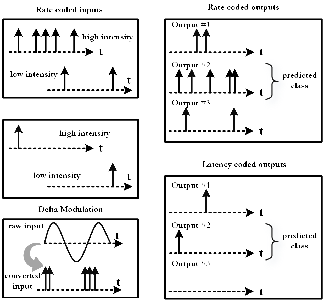
All network topologies used in the upcoming numerical examples follow a general scheme, which is flexible and suited for regression tasks. First, the real input $\bm{x}_{t}$ is provided as a constant input to the first layer $\bm{h}_{t}^{(0)}$ , for all time steps $t$ , such that

\bm{h}_{t}^{(0)}\left(\bm{x}_{t}\right)=\bm{h}_{t}^{\text{const}}\left(\bm{x}_{t}\right)=\bm{x}_{t}\;\forall\;t\in\left[0,d_{t}\right].

((10))

Then, several SNN layers $\bm{h}_{t}^{(l)}$ follow, where the exact formulation is arbitrary, and will be given for every numerical example. The output of the last spiking layer $\bm{h}_{t}^{(n_{L})}$ is transformed into a decoding layer $\bm{h}_{t}^{\text{dec}}$ , which takes the membrane potential of every time step as input and outputs real numbers

\bm{h}_{t}^{\text{dec}}=\beta_{\eta}^{(l)}U_{\eta,t-1}^{(l)}+\bm{W}^{(l)}_{\eta}\bm{h}_{t}^{(l-1)},

((11))

which is essentially the formulation of Eq. (7), where no spikes and reset mechanisms are used. The transformed values are then transferred to the ‘population voting layer’, where the output of all neurons of the decoding layer are averaged to give real numbers. This results in

\bm{h}_{t}^{\text{pop}}=\frac{1}{n_{o}}\sum_{n_{o}}\left(\beta_{\eta}^{(l)}U_{\eta,t-1}^{(l)}+\bm{W}^{(l)}_{\eta}\bm{h}_{t}^{(l-1)}\right),

((12))

where $n_{o}$ denotes the number of neurons in the population voting layer and again, no spikes or reset mechanisms are used.

The final spiking regression topology network $\mathcal{S}$ can be written as

$\displaystyle\mathcal{S}:\mathbb{R}^{d_{t}\times d_{x}}$	$\displaystyle\to\mathbb{R}^{d_{t}\times d_{y}}$	((13))
$\displaystyle\bm{x}_{t}$	$\displaystyle\mapsto\bm{h}_{t}^{\text{pop}}\circ\bm{h}_{t}^{\text{dec}}\circ\bm{h}_{t}^{(n_{L})}\circ\ldots\circ\bm{h}_{t}^{(l)}\circ\ldots$
	$\displaystyle\ldots\circ\bm{h}_{t}^{(1)}\circ\bm{h}_{t}^{\text{const}}\left(\bm{x}_{t}\right)=\bm{y}_{t}.$

To summarize, information flows in the form of constant current (real numbers) into the input layer $\bm{h}_{t}^{\text{const}}$ , is then transformed into binary spikes in the spiking layers $\bm{h}_{t}^{(l)}$ and transformed back into real numbers in the translation layer $\bm{h}_{t}^{\text{dec}}$ . The output is formed in the population layer $\bm{h}_{t}^{\text{pop}}$ . A graphical interpretation is given in Figure 6.

Fig. 6: Topology of the spiking regression network introduced in Section II-A.

For all the following numerical examples, the AdamW optimizer from [95] is used. The parameter are set as follows: learning rate $\alpha=1\times 10^{-3}$ , exponential decay rates for the first and second moment estimates $\beta_{1}=0.9$ and $\beta_{2}=0.999$ , respectively, weight decay $\lambda=0.01$ . The training was carried out on a Nvidia GeForce RTX 3090 GPU using snnTorch [62] and PyTorch [61]. In this work, the mean relative error $\mathcal{E}$ is used, which is defined as

\mathcal{E}_{\bullet}(\bullet)=\frac{1}{n_{s}}\displaystyle\sum_{i=1}^{n_{s}}\frac{||\hat{{\bullet}}_{i}-{\bullet}_{i}||_{2}}{||\hat{{\bullet}}_{i}||_{2}},

((14))

for some input $\bullet$ and baseline $\hat{\bullet}$ . If the error is reported for all time steps, $\bullet$ is a vector containing the values of all time steps. If the error is reported for the last time step, $\bullet$ is equal to the last component of the corresponding history-dependent vector.

II-B Numerical experiment: Linear elasticity

The first study investigates the effect of the number of time steps on the performance of the proposed LIF topology in a simple linear regression problem. To this end, the general model described in Section II-A with LIF defined in Eq. (7) is used, resulting in the following network topology

\mathcal{S}\left(\varepsilon_{t}\right)=\bm{h}_{t}^{\text{pop}}\circ\bm{h}_{t}^{\text{dec}}\circ\bm{h}_{t}^{\text{LIF}}\circ\bm{h}_{t}^{\text{LIF}}\circ\bm{h}_{t}^{\text{LIF}}\circ\bm{h}_{t}^{\text{const}}\left(\varepsilon_{t}\right)=\sigma_{t}.

((15))

To begin with, a simple linear elastic material model with strains in the range of $\varepsilon=[0,0.001]$ and fixed Young’s modulus $E=2.1\times 10^{5}$ MPa is considered, such that the resulting stress $\sigma$ is

\sigma=E\varepsilon.

((16))

The training data consists of strain input, uniformly sampled in the interval $\varepsilon=[0,0.001]$ , and stress output calculated according to Eq. (16). Three datasets are generated, namely a training set, a validation and a test set consisting each of $n_{\text{train}}=n_{\text{val}}=n_{\text{test}}=1024$ samples. All three datasets are standardized using the mean and standard deviation from the training set. The batch size is chosen as $n_{\text{batch}}=1024$ . The number of neurons $n_{u}$ is chosen as $n_{u}=128$ and is kept constant over all layers. The training is carried out for $2\times 10^{3}$ epochs. The model performing best on the validation set is chosen for subsequent evaluations. The mean relative error accumulated over all time steps and the mean relative error of the last time step with respect to the test set are reported.

The results are illustrated in Figure 7. It can be seen, that the mean relative error is lowest for $d_{t}=5$ time steps. For $d_{t}=2$ , the error is larger. This could be caused by a lack of a sufficient number of time steps for the neuron dynamics to effectively be calculated. It can be understood as a failure due to too large time steps in the explicit stepping scheme in Eq. (7). Clearly, the highest error can be observed for $d_{t}=100$ time steps. In contrast, as depicted in Figure 8, the error at the last time step is lowest for $d_{t}=100$ time steps. To illustrate the cause, the prediction of the network for two different samples, one for $d_{t}=5$ and one for $d_{t}=100$ time steps are shown in Figure 9 and Figure 10, respectively. While good agreement on the endpoints is apparent, fluctuation during the rest of the time steps causes the rise in the error. Seemingly, the LIF has difficulties regressing a large number of time steps. This could be caused by the lack of recurrent connections in the LIF formulation from Eq. (15), where history dependency is only weakly included in the form of the membrane potential. To counter this problem, recurrent LIFs will be introduced in Section III.

Remark: The seemingly simple linear regression task provides a challenge for SNN, as effectively an ordinary differential equation has to be fitted to a linear function while relying on binary information transmission and inexact gradients.

Fig. 7: Elasticity - error of all timesteps: Mean relative error for all time steps with respect to the different total number of time steps. The error is rising for a larger number of time steps.

Fig. 8: Elasticity - error at last time step: Mean relative error for the last time step with respect to the different total number of time steps. The error is converging for a larger number of time steps.

Fig. 9: Elasticity - prediction in 5 time steps: Prediction of the LIF from Eq. (15) for

d_{t}=5

. Deviations from the true solution can be observed in the middle part.

Fig. 10: Elasticity - prediction in 100 time steps: Prediction of the LIF from Eq. (15) for

d_{t}=100

. Fluctuations around the true solution can be observed.

III Nonlinear regression using RLIF

In order to counter the problems of vanishing information for a large number of time steps encountered in the preceding section, a recurrent SNN architecture is proposed (Section III-A). Its performance is demonstrated by means of a numerical example in Section III-B.

III-A Recurrent Leaky Integrate and Fire (RLIF)

The standard LIF is a feed-forward neuron, such that information is flowing unidirectionally in the form of spikes. By adding a feedback loop, a recurrent LIF (RLIF) can be formulated, which builds on the standard recurrent neural network (RNN) formulation. This enables the network to use relationships along several time steps for the prediction of the current time step. It was shown in [96], that recurrent loops can retain information for a relatively longer number of time steps when compared to their non-recurrent counterparts.

Here, the formulation of the hidden layer in Eq. (5) includes additional recurrent weights $\bm{V}^{(l)}_{\eta}$ , such that

h_{\eta,t}^{(l)}=\phi^{(l)}\left(\bm{W}^{(l)}_{\eta}\bm{h}_{t}^{(l-1)}+\bm{V}^{(l)}_{\eta}\bm{h}_{t-1}^{(l-1)}\right).

((17))

In this RNN, the influence of the preceding time step is explicitly included by means of additional recurrent weights $\bm{V}^{(l)}_{\eta}$ . The resulting set of trainable parameters reads

\bm{\theta}_{\text{RNN}}=\left\{\bm{W}_{\eta}^{(l)},\bm{V}^{(l)}_{\eta}\right\}.

((18))

The RNN formulation can be included in the LIF formulation from Eq. (7) to obtain an RLIF, such that

	$\displaystyle U_{\eta,t}^{(l)}$	$\displaystyle=\beta_{\eta}^{(l)}U_{\eta,t-1}^{(l)}+\bm{W}^{(l)}_{\eta}\bm{h}_{t}^{(l-1)}$		((19))
		$\displaystyle\quad+\bm{V}^{(l)}_{\eta}\bm{h}_{t-1}^{(l-1)}-\phi_{\text{spk},t-1}^{(l)}U_{\text{thr},\eta}^{(l)},$

where $U_{\eta,t}^{(l)}$ is again the membrane potential of the $\eta$ -th neural unit at time $t$ , $U_{\text{thr},\eta}^{(l)}$ denotes the membrane threshold, $\beta_{\eta}^{(l)}$ is the membrane potential decay rate and $\bm{W}^{(l)}_{\eta}\bm{h}_{t}^{(l-1)}$ is the standard ANN weight multiplied with the preceding layer at the current time step, respectively. Additionally, $\bm{V}^{(l)}_{\eta}$ denotes the recurrent weights from Eq. (17). This leads to the following set of trainable parameters

\bm{\theta}_{\text{RLIF}}=\left\{\bm{W}_{\eta}^{(l)},\bm{V}^{(l)}_{\eta},\beta_{\eta}^{(l)},U_{\text{thr},\eta}^{(l)}\right\}.

((20))

III-B Numerical experiment: Ramberg-Osgood

The performance of the RLIF is investigated toward nonlinear function regression. The well-known nonlinear Ramberg-Osgood power law for modeling history-independent plasticity is chosen. The formulation of the stress $\sigma$ with respect to the strain $\varepsilon$ reads

\varepsilon=\frac{\sigma}{E}+0.002\left(\frac{\sigma}{\sigma_{Y}}\right)^{n},

((21))

where $\varepsilon$ is the infinitesimal, one-dimensional elastic strain, $\sigma$ denotes the one-dimensional Cauchy stress, $E$ is Young’s modulus, $\alpha$ and $n$ are constants describing the hardening behavior of plastic deformation and $\sigma_{Y}$ is the yield strength of the material. In Figure 11, different stress-strain curves are depicted for different yield strength values, obtained with a classical Newton-Raphson method. Note that this plasticity model is only suited for a single loading direction and does not incorporate accumulation of plastic strain. It is only used as a prototypical nonlinear model to show the ability of the RLIF to regress over a moderate number of time steps.

To this end, the general model described in Section II-A using RLIF defined in Eq. (19) is used, resulting in the following architecture

	$\displaystyle\mathcal{S}\left(\sigma_{Y}\right)$	$\displaystyle=\bm{h}_{t}^{\text{pop}}\circ\bm{h}_{t}^{\text{dec}}\circ\bm{h}_{t}^{\text{RLIF}}\circ\bm{h}_{t}^{\text{RLIF}}\circ\bm{h}_{t}^{\text{RLIF}}$		((22))
		$\displaystyle\quad\circ\bm{h}_{t}^{\text{const}}\left(\sigma_{Y}\right)=\sigma_{t},$

where the yield strength $\sigma_{Y}$ is provided as a constant current, that is a constant spike train, for each time step $d_{t}$ .

Fig. 11: Ramberg-Osgood - reference solutions. Stress-strain curves of the Ramberg-Osgood material model for five different values of the yield stress

\sigma_{Y}

obtained with Newton-Raphson algorithm.

The training data consists of yield strength $\sigma_{Y}$ as input for fixed strains in the interval $\varepsilon=[0,0.01]$ for $d_{t}=20$ time steps. The yield strength is uniformly sampled in the interval $\sigma_{Y}=[100,500]$ MPa, and the stress output is calculated according to Eq. (21). The Young’s modulus is chosen as $E=2.1\times 10^{5}$ MPa and $n=10$ . Three datasets are generated, namely a training set, a validation and test set with $n_{\text{train}}=n_{\text{val}}=n_{\text{test}}=1024$ samples, respectively. All three sets are standardized using the mean and standard deviation from the training set. The batch size is chosen as $n_{\text{batch}}=1024$ . The number of neurons $n_{u}$ is chosen as $n_{u}=128$ and is kept constant over all layers. The training is carried out for $5\times 10^{3}$ epochs. The model performing best on the validation set is chosen for subsequent evaluations. The mean relative error and the mean relative error of the last time step with respect to the test set are reported.

The results of five different samples, randomly chosen from the $n_{test}=1024$ test samples, can be seen in Figure 13. For the test set, a mean relative error for all time steps of $8.7934\times 10^{-2}$ and a mean relative error for the last time step of $8.0200\times 10^{-2}$ is obtained. The predictions on these five samples are more accurate than would be suspected from the mean relative error. The cause can be found in Figure 12, where the mean relative error for all time steps is plotted for every sample of the test set. It can be observed, that a small number of samples has a much higher error than the rest, which impacts the error measure. This is caused by the purely data-driven nature of the experiment and can be tackled with approaches introduced in, e.g., [77, 78, 79]. Nevertheless, the RLIF is able to regress on the varying yield strength $\sigma_{Y}$ and can predict the resulting nonlinear stress-strain behavior, as can be seen in the predictions Figure 13. Deviations can be observed around the yield point as well as the endpoints of the curves. To be able to take into account long-term history dependent behavior, the RLIF formulation will be expanded towards the incorporation of explicit long-term memory in the next section, where a more complex plasticity model is investigated.

Fig. 12: Ramberg-Osgood - RLIF test error. The mean relative error over all time steps for 1024 samples from the test set for the numerical experiment described in Section III-B. It can be seen, that some outliers have large error values, resulting in a mean error over all samples of

8.7934\times 10^{-2}

. Most samples have a significantly lower error.

Fig. 13: Ramberg-Osgood - RLIF prediction. Prediction of the RLIF from Eq. (22) for five different yield strength

\sigma_{Y}

sampled from the test set for the nonlinear Ramberg-Osgood plasticity law.

IV History-dependent regression using SLSTM

To extend the limited memory of the RNN in Section III, a spiking long short-term memory neural network (SLSTM, Section IV-A) is investigated on a history-dependent plasticity model (Section IV-B).

IV-A Spiking long short-term memory network (SLSTM)

A SLSTM is the spiking version of the standard LSTM [97], where the latter is defined as

h_{\eta,t}^{(l)}=o_{\eta,t}^{(l)}\odot\phi_{\text{tanh}}\left(c_{\eta,t}^{(l)}\right),

((23))

with

	$\displaystyle o_{\eta,t}^{(l)}$	$\displaystyle=\phi_{\text{sigmoid}}\left(\bm{W}^{(l)}_{o,\eta}\bm{h}_{t}^{(l-1)}+\bm{V}^{(l)}_{o,\eta}\bm{h}_{t-1}^{(l-1)}\right),$
	$\displaystyle c_{\eta,t}^{(l)}$	$\displaystyle=f_{\eta,t}^{(l)}\odot c_{\eta,t-1}^{(l)}+i_{\eta,t}^{(l)}\odot\tilde{c}_{\eta,t}^{(l)},$
	$\displaystyle f_{\eta,t}^{(l)}$	$\displaystyle=\phi_{\text{sigmoid}}\left(\bm{W}^{(l)}_{f,\eta}\bm{h}_{t}^{(l-1)}+\bm{V}^{(l)}_{f,\eta}\bm{h}_{t-1}^{(l-1)}\right),$
	$\displaystyle i_{\eta,t}^{(l)}$	$\displaystyle=\phi_{\text{sigmoid}}\left(\bm{W}^{(l)}_{i,\eta}\bm{h}_{t}^{(l-1)}+\bm{V}^{(l)}_{i,\eta}\bm{h}_{t-1}^{(l-1)}\right),$
	$\displaystyle\tilde{c}_{\eta,t}^{(l)}$	$\displaystyle=\phi_{\text{tanh}}\left(\bm{W}^{(l)}_{c,\eta}\bm{h}_{t}^{(l-1)}+\bm{V}^{(l)}_{c,\eta}\bm{h}_{t-1}^{(l-1)}\right),$

where $f_{t}$ denotes the forget gate with sigmoid activation $\phi_{\text{sigmoid}}$ or tangent hyperbolicus activation $\phi_{\text{tanh}}$ and corresponding weights $\bm{W}_{f},\bm{V}_{f}$ with absorbed biases. The same nomenclature holds for the input gate $i_{t}$ , the output gate $o_{t}$ , the cell input $\tilde{c}_{t}$ and the cell state $c_{t}$ with their respective activations and weights. The new cell state $c_{t}$ and the output of the LSTM $h_{t}$ are formed using the Hadamard or point-wise product $\odot$ . The parameters of the LSTM are its weights, such that

	$\displaystyle\bm{\theta}_{\text{LSTM}}=\Big\{$	$\displaystyle\bm{W}^{(l)}_{f,\eta},\bm{W}^{(l)}_{i,\eta},\bm{W}^{(l)}_{o,\eta},\bm{W}^{(l)}_{c,\eta},$		((24))
		$\displaystyle\bm{V}^{(l)}_{f,\eta},\bm{V}^{(l)}_{i,\eta},\bm{V}^{(l)}_{o,\eta},\bm{V}^{(l)}_{c,\eta}.\Big\}.$

For detailed derivations and explanations of standard LSTM, see, e.g., [87, 88]. The SLSTM can be obtained from the LSTM by using spike activations within the LSTM formulation from Eq. (23), such that

h_{\eta,t}^{(l)}=o_{\eta,t}^{(l)}\odot\phi_{\text{tanh}}\left(c_{\eta,t}^{(l)}\right){-\phi_{\text{spk},t-1}^{(l)}U_{\text{thr},\eta}^{(l)}},

((25))

where the output $h_{\eta,t}^{(l)}$ is used to determine if a spike is produced

\displaystyle\phi_{\text{spk},t}^{(l)}=\begin{cases}1,\quad h_{\eta,t}^{(l)}\geq U_{\text{thr},\eta}^{(l)}\\ 0,\quad h_{\eta,t}^{(l)}<U_{\text{thr},\eta}^{(l)}.\end{cases}

((26))

In other words, the output of $h_{\eta,t}^{(l)}$ can be interpreted as the membrane potential of the SLSTM, such that $h_{\eta,t}^{(l)}=U_{\eta,t}^{(l)}$ . A decay parameter $\beta$ is not used in this formulation. Rather than using decay to remove information from the cell state $c_{\eta,t}^{(l)}$ , this is achieved by carefully regulated gates.

The corresponding optimization parameters of the SLSTM are

	$\displaystyle\bm{\theta}_{\text{SLSTM}}=\Big\{$	$\displaystyle\bm{W}^{(l)}_{f,\eta},\bm{W}^{(l)}_{i,\eta},\bm{W}^{(l)}_{o,\eta},\bm{W}^{(l)}_{c,\eta},$		((27))
		$\displaystyle\bm{V}^{(l)}_{f,\eta},\bm{V}^{(l)}_{i,\eta},\bm{V}^{(l)}_{o,\eta},\bm{V}^{(l)}_{c,\eta},U_{\text{thr},\eta}^{(l)}\Big\}.$

Basically, the cell state $c_{\eta,t}^{(l)}$ acts as long-term memory, just like in the standard LSTM formulation. The communication between layers is handled via spike trains that depend on the membrane potential $h_{\eta,t}^{(l)}=U_{\eta,t}^{(l)}$ in Eq. (25) and the activation function $\phi_{\text{spk},t}^{(l)}$ from Eq. (26).

IV-B Numerical experiment: Isotropic hardening using SLSTM

The following numerical experiments aim to investigate the performance of the proposed SLSTM on nonlinear, history-dependent problems. Therefore, a one-dimensional plasticity model with isotropic hardening is investigated. Following [98], the model is defined by

		$\displaystyle 1.\quad\varepsilon=\varepsilon_{\text{el}}+\varepsilon_{\text{pl}},$		((28))
		$\displaystyle 2.\quad\sigma=E\left(\varepsilon-\varepsilon_{\text{pl}}\right),$
		$\displaystyle 3.\quad\dot{\varepsilon}_{\text{pl}}=\gamma\operatorname{sign}\left(\sigma\right),\quad\dot{\alpha}=\gamma,$
		$\displaystyle 4.\quad f\left(\sigma,\alpha\right)=\|\sigma\|-\left(\sigma_{Y}+K\alpha\right)\leq 0,$
		$\displaystyle 5.\quad\gamma\geq 0,\quad f\left(\sigma,\alpha\right)\leq 0,\quad\gamma f\left(\sigma,\alpha\right)=0,$
		$\displaystyle 6.\quad\gamma\dot{f}\left(\sigma,\alpha\right)=0,\quad\text{if}\;f\left(\sigma,\alpha\right)=0,$

where

1.

is the additive elasto-plastic split of the small-strain tensor $\varepsilon$ into a purely elastic part $\varepsilon_{\text{el}}$ and a purely plastic part $\varepsilon_{\text{el}}$ .
2.

denotes the elastic stress-strain relationship for the Cauchy stress tensor $\sigma$ and elastic modulus $E$ .
3.

describes the flow rule and isotropic hardening law with consistency parameter $\gamma$ and equivalent plastic strain $\alpha$ .
4.

gives the yield condition $f\left(\sigma,\alpha\right)$ with hardening modulus $K$ .
5.

denotes the Kuhn-Tucker complementarity conditions and
6.

describes the consistency condition.

In Figure 14, different stress-strain paths are shown for varying strains. Especially long-time dependencies are of interest. To this end, the predictive capabilities of the SNN are investigated for inference over $d_{t}=100$ time steps, where the elasto-plastic model is evaluated using a classical explicit return-mapping algorithm, see [98].

Fig. 14: Isotropic hardening - reference solutions. Five stress-strain curves sampled from the isotropic hardening material model for different maximum strains obtained from Eq. (28).

The training data consists of strain as input, uniformly sampled in the interval $\varepsilon=[0,0.01]$ , and stress as output calculated according to Eq. (28). The yield stress is chosen as $\sigma_{Y}=300$ MPa, the elastic modulus $E=2.1\times 10^{5}$ MPa and the hardening modulus as $2.1\times 10^{4}$ MPa. Three datasets are generated, namely a training set with $n_{\text{train}}=10240$ samples and a validation and test set with $n_{\text{val}}=n_{\text{test}}=1024$ samples, respectively. All three sets are standardized using the mean and standard deviation from the training set. The batch size is chosen as $n_{\text{batch}}=1024$ . The training is carried out for 500 epochs. The model performing best on the validation set is chosen for subsequent evaluations. The mean relative error accumulated over all time steps and the mean relative error of the last time step with respect to the test set are reported. The last time step is of special importance, as in the case of numerical simulations, only the resulting stress from the last time step is used for subsequent calculations.

The first study investigates the prediction accuracy as a function of (1) the number of output neurons, which participate in the population regression outlined in Section II-A and (2) different capacities of the SLSTM in the sense of layer width. To this end, the SLSTM defined in Eq. (26) is used, resulting in the following architecture:

	$\displaystyle\mathcal{S}_{\textit{SLSTM}}\left(\varepsilon_{t}\right)$	$\displaystyle=\bm{h}_{t}^{\text{pop}}\circ\bm{h}_{t}^{\text{dec}}\circ\bm{h}_{t}^{\text{SLSTM}}\circ\bm{h}_{t}^{\text{SLSTM}}\circ\bm{h}_{t}^{\text{SLSTM}}$		((29))
		$\displaystyle\quad\circ\bm{h}_{t}^{\text{const}}\left(\varepsilon_{t}\right)=\sigma_{t}.$

Multiple simulations with output neurons and hidden layers drawn from the grid $n_{u}\times n_{o}=[16,32,64,128,256]\times[16,32,64,128,256]$ are carried out. The resulting mean relative error for all time steps with respect to the test set is shown in Figure 15, whereas the resulting mean relative error of the last time step with respect to the test set is depicted in Figure 16. A clear convergence behavior can be observed for the number of hidden neurons $n_{u}$ , where larger numbers of neurons lead to lower errors. For the number of output neurons $n_{o}$ , a tendency can be observed upon convergence with respect to $n_{u}$ . For the largest number of hidden neurons $n_{u}=256$ , the mean relative error over all time steps and the mean relative error of the last time step get larger for $n_{o}=[128,256]$ output neurons, whereas for $n_{o}=[16,32,64]$ the errors are almost the same. The lowest mean relative error for all time steps is $5.2445\times 10^{-2}$ for $n_{u}=256$ hidden neurons per layer and $n_{o}=64$ output neurons. The lowest mean relative error for the last time steps is $2.8729\times 10^{-3}$ $n_{u}=256$ hidden neurons per layer and $n_{o}=32$ output neurons. Again, the seemingly high errors are caused by outliers polluting the average, as described in Section III-B. The same counter-measures can be applied to prohibit outliers, e.g., by enforcing thermodynamic consistency.

Fig. 15: Isotropic hardening - error versus width. The mean relative error of the last time step versus the number of hidden neurons per layer is shown for different numbers of output neurons in the isotropic hardening experiment from Section IV using the SLSTM from Eq. (29).

Fig. 16: Isotropic hardening - error versus width. The mean relative error of all time steps versus the number of hidden neurons per layer is shown for different numbers of output neurons in the isotropic hardening experiment from Section IV using the SLSTM from Eq. (29).

For the second experiment, the SLSTM using $n_{o}=64$ output neurons and $n_{u}=256$ hidden neurons per layer are compared to a standard LSTM with an equal number of optimization parameters. The aim of this study is the comparison of the prediction accuracy, but also the difference in memory and energy consumption on neuromorphic hardware. For both ANN variants to be comparable, the same topology is chosen for the LSTM as for the SLSTM, such that

	$\displaystyle\mathcal{N}_{\textit{LSTM}}\left(\varepsilon_{t}\right)$	$\displaystyle=\bm{h}_{t}^{\text{dense}}\circ\bm{h}_{t}^{\text{dense}}\circ\bm{h}_{t}^{\text{LSTM}}\circ\bm{h}_{t}^{\text{LSTM}}\circ\bm{h}_{t}^{\text{LSTM}}$		((30))
		$\displaystyle\quad\circ\bm{h}_{t}^{\text{const}}\left(\varepsilon_{t}\right)=\sigma_{t},$

where the last two layers are replaced by densely connected conventional feed-forward neural networks. Again, the training was carried out for $5\times 10^{3}$ epochs and the same datasets from the previous experiments are used. The standard LSTM from Eq. (30) reached a mean relative error of $4.8611\times 10^{-2}$ over all time steps and a mean relative error of $4.7569\times 10^{-3}$ for the last time step. The SLSTM from Eq. (29) reached a mean relative error of $9.3832\times 10^{-2}$ over all time steps and a mean relative error of $4.0497\times 10^{-3}$ for the last time step. The resulting prediction for one strain path is illustrated in Figure 17. Clearly, both networks are able to accurately predict the history-dependent, nonlinear stress-strain behavior.

Some deviations from the SLSTM can be seen in the beginning of the curve. The dynamics of the spiking formulation results in a higher mean relative error over all time steps with respect to the LSTM. However, the endpoint has a better fit than the LSTM. This is seen in the lower error at the last time step. Whether this is just an effect due to our experimental setting or a general feature of the method has to be investigated in a larger statistical analysis in upcoming studies.

To assess the potential of interfacing our model in embedded, resource-constrained sensors in the wild, we performed a series of power profiling experiments for our SNNs (both using LIF neurons and SLSTMs) when processed on the Loihi neuromorphic chip [53]. These results are compared against their non-spiking equivalents on an NVIDIA V100 GPU. Data were extracted using the energy profiler in KerasSpiking v0.3.0.

The first difference in energy usage is that the spiking implementation is measured in an ‘event-based’ manner, where processing only occurs when a neuron emits a spike. In contrast, a non-spiking network processed on a GPU continuously computes with all activations. Note that the cost of overhead did not need to be accounted for (i.e., transferring data between devices) because all models fit on a single device. The second difference is that SNNs require multiple time steps of a forward pass, whereas their non-spiking counterparts do not (unless the input to the network varies over time).

Architecture	Energy		Architecture	Energy
Dense	Loihi (nJ)	GPU (nJ)	LSTM	Loihi (nJ)	GPU (nJ)
$\mathbin{\vbox{\hbox{\scalebox{.5}{$\bullet$}}}}$ FC1	6.9e-2	0.61	$\mathbin{\vbox{\hbox{\scalebox{.5}{$\bullet$}}}}$ LSTM1	0.28	2.5
$\mathbin{\vbox{\hbox{\scalebox{.5}{$\bullet$}}}}$ FC2	1.3	160	$\mathbin{\vbox{\hbox{\scalebox{.5}{$\bullet$}}}}$ LSTM2	11	2.5e3
$\mathbin{\vbox{\hbox{\scalebox{.5}{$\bullet$}}}}$ FC3	1.3	160	$\mathbin{\vbox{\hbox{\scalebox{.5}{$\bullet$}}}}$ LSTM3	10	2.5e3
$\mathbin{\vbox{\hbox{\scalebox{.5}{$\bullet$}}}}$ FC4	1.2	160	$\mathbin{\vbox{\hbox{\scalebox{.5}{$\bullet$}}}}$ FC1	2.6	630
$\mathbin{\vbox{\hbox{\scalebox{.5}{$\bullet$}}}}$ FC5	0.3	39	$\mathbin{\vbox{\hbox{\scalebox{.5}{$\bullet$}}}}$ FC2	0.21	39
Total Energy	4.25	512	Total Energy	24	5.7e3
Reduction	$\times$ 120		Reduction Factor	$\times$ 238
Synaptic Memory	0.86 MB		Synaptic Memory	9.5 MB

TABLE I: Comparison between spiking and non-spiking forward-pass energy consumption and memory usage.

Each network has been broken up into its constituent layers to measure how much they contribute to energy usage on each device. The total energy consumption per forward pass of the non-spiking network on the V100 is 512 nJ, whereas the equivalent SNN is 4.25 nJ. This represents a 120x reduction in energy consumption. The non-spiking LSTM network consumed 5.7 $\mu$ J while the proposed spiking-LSTM architecture required 24 nJ, a 238 $\times$ reduction. Detailed results are summarized in Table I.

Fig. 17: Isotropic hardening - LSTM versus SLSTM. Prediction of a single load path using the return-mapping algorithm as a reference, the standard LSTM and the spiking LSTM formulation.

V Conclusion and outlook

In the present study a framework for regression using SNNs was proposed based on a membrane potential spiking decoder and a population voting layer. Several numerical examples using different spiking neural architectures investigated the performance of the introduced topology towards linear, nonlinear, and history-dependent regression problems.

First, a simple feed-forward SNN, the LIF, was derived from the classical densely connected feed-forward ANN. It was shown, that the SNN can be seen as a special kind of activation function, which produces binary outputs, so-called spikes. These spikes are used to propagate information through a possibly deep spiking neural network. The spikes occur due to the dynamic behavior of the membrane potential inside the neuron, which rises when spikes appear at the input and decays over time if no spikes appear. If a certain threshold value is reached, the membrane potential is reset and the neuron emits a spike itself. This formulation introduces more hyperparameters, which fortunately can be learned during training. The spikes introduce sparsity in the network, which can be effectively exploited by neuromorphic hardware to improve latency, power, and memory efficiency. The non-differentiability of the binary spikes is circumvented by surrogate gradients during backpropagation.

Next, a network topology was proposed, which decodes binary spikes into real numbers, which is essential for all kinds of regression problems. A decoding layer takes the membrane potentials of all neurons in the last spiking layer and propagates them to a population voting layer, which provides its mean potential resulting in a real number. The proposed topology can be used for arbitrary temporal input and output dimensions. A simple experiment on a linear elastic material model using LIFs showed, that the proposed topology is able to regress the problem. It was shown, that errors are introduced for a large number of time steps. This problem was overcome by introducing RLIF, which extends the LIF by recurrent feedback loops. An experiment using a nonlinear Ramberg-Osgood plasticity model showed that the proposed topology using RLIF is able to regress varying yield limits accurately. The final extension was concerned with the introduction of explicit long-term memories inspired by the classical LSTM formulation, resulting in a spiking LSTM. The performance of this SLSTM was investigated on a history-dependent isotropic hardening model, where different load paths were accurately regressed. During prediction, the SLSTM was able to generalize even better than the LSTM for the final load step. Furthermore, the convergence of the proposed method was shown.

Power profiling and memory analysis were conducted on the LIF and SLSTM networks to compare efficiency on neuromorphic hardware as against a GPU. The Loihi neuromorphic processor was able to achieve a 120 $\times$ reduction in energy consumption when processing the dense LIF network, and the SLSTM offered a 238 $\times$ reduction in energy during inference.

The range of possible future application scenarios enabled by regression with Spiking Neural Networks are manifold. For instance, today’s sensing systems cannot capture all quantities that are relevant for structural health-monitoring. In the context of mechanics, displacement and strain are quiet easy to assess, but the mechanical stress, which reflects the actual response of structures and materials to deformation, remains a so-called hidden-quantity. Physics-informed machine learning offers the potential to reconstruct hidden quantities from data by leveraging information from physical models, given in the form of partial differential equations. It is expected that the developments in the field of neuromorphic hardware will foster the development of a new generation of embedded systems, which will ultimately enable control of structures and processes based on partial differential equations.

Declaration of competing interest

The authors declare that they have no known competing financial interests or personal relationships that could have appeared to influence the work reported in this paper.

Data availability

The code will be available upon acceptance at https:github.com/ahenkes1/HENKES_SNN and [henkes_code_snn_ZENODO].

References

[1] K. Hornik, M. Stinchcombe, and H. White, “Multilayer feedforward networks are universal approximators,” Neural networks, vol. 2, no. 5, pp. 359–366, 1989.
[2] G. Cybenko, “Approximation by superpositions of a sigmoidal function,” Mathematics of control, signals and systems, vol. 2, no. 4, pp. 303–314, 1989.
[3] T. Chen and H. Chen, “Universal approximation to nonlinear operators by neural networks with arbitrary activation functions and its application to dynamical systems,” IEEE Transactions on Neural Networks, vol. 6, no. 4, pp. 911–917, 1995.
[4] J. Berner, P. Grohs, G. Kutyniok, and P. Petersen, “The modern mathematics of deep learning,” arXiv preprint arXiv:2105.04026, 2021.
[5] J. N. Kutz, “Deep learning in fluid dynamics,” Journal of Fluid Mechanics, vol. 814, pp. 1–4, 2017.
[6] W.-W. Zhang and B. R. Noack, “Artificial intelligence in fluid mechanics,” Acta Mechanica Sinica, vol. 37, no. 12, pp. 1715–1717, 2021.
[7] S. Cai, Z. Mao, Z. Wang, M. Yin, and G. E. Karniadakis, “Physics-informed neural networks (pinns) for fluid mechanics: A review,” Acta Mechanica Sinica, pp. 1–12, 2022.
[8] M. Raissi, A. Yazdani, and G. E. Karniadakis, “Hidden fluid mechanics: Learning velocity and pressure fields from flow visualizations,” Science, vol. 367, no. 6481, pp. 1026–1030, 2020.
[9] H. Wessels, C. Weißenfels, and P. Wriggers, “The neural particle method–an updated lagrangian physics informed neural network for computational fluid dynamics,” Computer Methods in Applied Mechanics and Engineering, vol. 368, p. 113127, 2020.
[10] E. Haghighat, M. Raissi, A. Moure, H. Gomez, and R. Juanes, “A physics-informed deep learning framework for inversion and surrogate modeling in solid mechanics,” Computer Methods in Applied Mechanics and Engineering, vol. 379, p. 113741, 2021.
[11] G. Buffa, L. Fratini, and F. Micari, “Mechanical and microstructural properties prediction by artificial neural networks in fsw processes of dual phase titanium alloys,” Journal of Manufacturing Processes, vol. 14, no. 3, pp. 289–296, 2012.
[12] D. W. Abueidda, Q. Lu, and S. Koric, “Meshless physics-informed deep learning method for three-dimensional solid mechanics,” International Journal for Numerical Methods in Engineering, vol. 122, no. 23, pp. 7182–7201, 2021.
[13] Z. Nie, H. Jiang, and L. B. Kara, “Stress field prediction in cantilevered structures using convolutional neural networks,” Journal of Computing and Information Science in Engineering, vol. 20, no. 1, p. 011002, 2020.
[14] A. Henkes, I. Caylak, and R. Mahnken, “A deep learning driven pseudospectral PCE based FFT homogenization algorithm for complex microstructures,” Computer Methods in Applied Mechanics and Engineering, vol. 385, p. 114070, 2021.
[15] A. Henkes, H. Wessels, and R. Mahnken, “Physics informed neural networks for continuum micromechanics,” Computer Methods in Applied Mechanics and Engineering, vol. 393, p. 114790, 2022.
[16] J. R. Mianroodi, N. H Siboni, and D. Raabe, “Teaching solid mechanics to artificial intelligence—a fast solver for heterogeneous materials,” Npj Computational Materials, vol. 7, no. 1, pp. 1–10, 2021.
[17] H. Wessels, C. Böhm, F. Aldakheel, M. Hüpgen, M. Haist, L. Lohaus, and P. Wriggers, “Computational homogenization using convolutional neural networks,” in Current Trends and Open Problems in Computational Mechanics. Springer, 2022, pp. 569–579.
[18] H. Dehghani and A. Zilian, “Poroelastic model parameter identification using artificial neural networks: on the effects of heterogeneous porosity and solid matrix poisson ratio,” Computational Mechanics, vol. 66, no. 3, pp. 625–649, 2020.
[19] P. Thakolkaran, A. Joshi, Y. Zheng, M. Flaschel, L. De Lorenzis, and S. Kumar, “Nn-euclid: deep-learning hyperelasticity without stress data,” arXiv preprint arXiv:2205.06664, 2022.
[20] E. Zhang, M. Yin, and G. E. Karniadakis, “Physics-informed neural networks for nonhomogeneous material identification in elasticity imaging,” arXiv preprint arXiv:2009.04525, 2020.
[21] E. Zhang, M. Dao, G. E. Karniadakis, and S. Suresh, “Analyses of internal structures and defects in materials using physics-informed neural networks,” Science advances, vol. 8, no. 7, p. eabk0644, 2022.
[22] D. Anton and H. Wessels, “Identification of material parameters from full-field displacement data using physics-informed neural networks,” Researchgate Preprint, 2021.
[23] F. As’ ad, P. Avery, and C. Farhat, “A mechanics-informed artificial neural network approach in data-driven constitutive modeling,” International Journal for Numerical Methods in Engineering, vol. 123, no. 12, pp. 2738–2759, 2022.
[24] H. Yang, H. Qiu, Q. Xiang, S. Tang, and X. Guo, “Exploring elastoplastic constitutive law of microstructured materials through artificial neural network—a mechanistic-based data-driven approach,” Journal of Applied Mechanics, vol. 87, no. 9, p. 091005, 2020.
[25] K. Xu, D. Z. Huang, and E. Darve, “Learning constitutive relations using symmetric positive definite neural networks,” Journal of Computational Physics, vol. 428, p. 110072, 2021.
[26] M. Fernández, S. Rezaei, J. Rezaei Mianroodi, F. Fritzen, and S. Reese, “Application of artificial neural networks for the prediction of interface mechanics: a study on grain boundary constitutive behavior,” Advanced Modeling and Simulation in Engineering Sciences, vol. 7, no. 1, pp. 1–27, 2020.
[27] F. Aldakheel, R. Satari, and P. Wriggers, “Feed-forward neural networks for failure mechanics problems,” Applied Sciences, vol. 11, no. 14, p. 6483, 2021.
[28] S.-W. Liu, J. H. Huang, J.-C. Sung, and C. Lee, “Detection of cracks using neural networks and computational mechanics,” Computer methods in applied mechanics and engineering, vol. 191, no. 25-26, pp. 2831–2845, 2002.
[29] A. Henkes and H. Wessels, “Three-dimensional microstructure generation using generative adversarial neural networks in the context of continuum micromechanics,” arXiv preprint arXiv:2206.01693, 2022.
[30] T. Hsu, W. K. Epting, H. Kim, H. W. Abernathy, G. A. Hackett, A. D. Rollett, P. A. Salvador, and E. A. Holm, “Microstructure generation via generative adversarial network for heterogeneous, topologically complex 3d materials,” JOM, vol. 73, no. 1, pp. 90–102, 2021.
[31] L. Mosser, O. Dubrule, and M. J. Blunt, “Reconstruction of three-dimensional porous media using generative adversarial neural networks,” Physical Review E, vol. 96, no. 4, p. 043309, 2017.
[32] J. Ma, S. Dong, G. Chen, P. Peng, and L. Qian, “A data-driven normal contact force model based on artificial neural network for complex contacting surfaces,” Mechanical Systems and Signal Processing, vol. 156, p. 107612, 2021.
[33] E. Öner, B. Şengül Şabano, E. Uzun Yaylacı, G. Adıyaman, M. Yaylacı, and A. Birinci, “On the plane receding contact between two functionally graded layers using computational, finite element and artificial neural network methods,” ZAMM-Journal of Applied Mathematics and Mechanics/Zeitschrift für Angewandte Mathematik und Mechanik, vol. 102, no. 2, p. e202100287, 2022.
[34] M. M. Ardestani, Z. Chen, L. Wang, Q. Lian, Y. Liu, J. He, D. Li, and Z. Jin, “Feed forward artificial neural network to predict contact force at medial knee joint: Application to gait modification,” Neurocomputing, vol. 139, pp. 114–129, 2014.
[35] Z. Feng, J. Yan, and Y. Gao, “Prediction of contact resistance between copper blocks under cyclic load based on deep learning algorithm,” AIP Advances, vol. 12, no. 7, p. 075009, 2022.
[36] S. Cai, Z. Wang, S. Wang, P. Perdikaris, and G. E. Karniadakis, “Physics-informed neural networks for heat transfer problems,” Journal of Heat Transfer, vol. 143, no. 6, 2021.
[37] R. Laubscher, “Simulation of multi-species flow and heat transfer using physics-informed neural networks,” Physics of Fluids, vol. 33, no. 8, p. 087101, 2021.
[38] H. R. Tamaddon-Jahromi, N. K. Chakshu, I. Sazonov, L. M. Evans, H. Thomas, and P. Nithiarasu, “Data-driven inverse modelling through neural network (deep learning) and computational heat transfer,” Computer Methods in Applied Mechanics and Engineering, vol. 369, p. 113217, 2020.
[39] S. A. Niaki, E. Haghighat, T. Campbell, A. Poursartip, and R. Vaziri, “Physics-informed neural network for modelling the thermochemical curing process of composite-tool systems during manufacture,” Computer Methods in Applied Mechanics and Engineering, vol. 384, p. 113959, 2021.
[40] V. A. Felipe Ramudo, “Machine learning to build reduced order models of solid mechanic models with uncertainty,” Master’s thesis, Universitat Politècnica de Catalunya, 2020.
[41] G. Balokas, S. Czichon, and R. Rolfes, “Neural network assisted multiscale analysis for the elastic properties prediction of 3d braided composites under uncertainty,” Composite Structures, vol. 183, pp. 550–562, 2018.
[42] J. N. Fuhg, I. Kalogeris, A. Fau, and N. Bouklas, “Interval and fuzzy physics-informed neural networks for uncertain fields,” Probabilistic Engineering Mechanics, vol. 68, p. 103240, 2022.
[43] A. Olivier, M. D. Shields, and L. Graham-Brady, “Bayesian neural networks for uncertainty quantification in data-driven materials modeling,” Computer Methods in Applied Mechanics and Engineering, vol. 386, p. 114079, 2021.
[44] F. E. Bock, R. C. Aydin, C. J. Cyron, N. Huber, S. R. Kalidindi, and B. Klusemann, “A review of the application of machine learning and data mining approaches in continuum materials mechanics,” Frontiers in Materials, vol. 6, p. 110, 2019.
[45] S. Kumar and D. M. Kochmann, “What machine learning can do for computational solid mechanics,” in Current Trends and Open Problems in Computational Mechanics, 2021.
[46] J. Blechschmidt and O. G. Ernst, “Three ways to solve partial differential equations with neural networks—a review,” GAMM-Mitteilungen, vol. 44, no. 2, p. e202100006, 2021.
[47] K. Roy, A. Jaiswal, and P. Panda, “Towards spike-based machine intelligence with neuromorphic computing,” Nature, vol. 575, no. 7784, pp. 607–617, 2019.
[48] G. Indiveri and S.-C. Liu, “Memory and information processing in neuromorphic systems,” Proceedings of the IEEE, vol. 103, no. 8, pp. 1379–1397, 2015.
[49] G. W. Burr, R. M. Shelby, A. Sebastian, S. Kim, S. Kim, S. Sidler, K. Virwani, M. Ishii, P. Narayanan, A. Fumarola et al., “Neuromorphic computing using non-volatile memory,” Advances in Physics: X, vol. 2, no. 1, pp. 89–124, 2017.
[50] N. Perez-Nieves and D. Goodman, “Sparse spiking gradient descent,” Advances in Neural Information Processing Systems, vol. 34, pp. 11 795–11 808, 2021.
[51] B. A. Olshausen and D. J. Field, “What is the other 85 percent of v1 doing,” L. van Hemmen, & T. Sejnowski (Eds.), vol. 23, pp. 182–211, 2006.
[52] W. Gerstner and W. M. Kistler, Spiking neuron models: Single neurons, populations, plasticity. Cambridge university press, 2002.
[53] M. Davies, N. Srinivasa, T.-H. Lin, G. Chinya, Y. Cao, S. H. Choday, G. Dimou, P. Joshi, N. Imam, S. Jain et al., “Loihi: A neuromorphic manycore processor with on-chip learning,” IEEE Micro, vol. 38, no. 1, pp. 82–99, 2018.
[54] S. B. Furber, F. Galluppi, S. Temple, and L. A. Plana, “The spinnaker project,” Proceedings of the IEEE, vol. 102, no. 5, pp. 652–665, 2014.
[55] P. A. Merolla, J. V. Arthur, R. Alvarez-Icaza, A. S. Cassidy, J. Sawada, F. Akopyan, B. L. Jackson, N. Imam, C. Guo, Y. Nakamura et al., “A million spiking-neuron integrated circuit with a scalable communication network and interface,” Science, vol. 345, no. 6197, pp. 668–673, 2014.
[56] M. R. Azghadi, C. Lammie, J. K. Eshraghian, M. Payvand, E. Donati, B. Linares-Barranco, and G. Indiveri, “Hardware implementation of deep network accelerators towards healthcare and biomedical applications,” IEEE Transactions on Biomedical Circuits and Systems, vol. 14, no. 6, pp. 1138–1159, 2020.
[57] C. Frenkel and G. Indiveri, “Reckon: A 28nm sub-mm² task-agnostic spiking recurrent neural network processor enabling on-chip learning over second-long timescales,” in 2022 IEEE International Solid-State Circuits Conference (ISSCC), vol. 65. IEEE, 2022, pp. 1–3.
[58] E. Ceolini, C. Frenkel, S. B. Shrestha, G. Taverni, L. Khacef, M. Payvand, and E. Donati, “Hand-gesture recognition based on emg and event-based camera sensor fusion: A benchmark in neuromorphic computing,” Frontiers in Neuroscience, vol. 14, p. 637, 2020.
[59] G. Orchard, E. P. Frady, D. B. D. Rubin, S. Sanborn, S. B. Shrestha, F. T. Sommer, and M. Davies, “Efficient neuromorphic signal processing with loihi 2,” in 2021 IEEE Workshop on Signal Processing Systems (SiPS). IEEE, 2021, pp. 254–259.
[60] M. Abadi, A. Agarwal, P. Barham, E. Brevdo, Z. Chen, C. Citro, G. S. Corrado, A. Davis, J. Dean, M. Devin, S. Ghemawat, I. Goodfellow, A. Harp, G. Irving, M. Isard, Y. Jia, R. Jozefowicz, L. Kaiser, M. Kudlur, J. Levenberg, D. Mané, R. Monga, S. Moore, D. Murray, C. Olah, M. Schuster, J. Shlens, B. Steiner, I. Sutskever, K. Talwar, P. Tucker, V. Vanhoucke, V. Vasudevan, F. Viégas, O. Vinyals, P. Warden, M. Wattenberg, M. Wicke, Y. Yu, and X. Zheng, “TensorFlow: Large-scale machine learning on heterogeneous systems,” 2015, software available from tensorflow.org. [Online]. Available: https://www.tensorflow.org/
[61] A. Paszke, S. Gross, F. Massa, A. Lerer, J. Bradbury, G. Chanan, T. Killeen, Z. Lin, N. Gimelshein, L. Antiga, A. Desmaison, A. Kopf, E. Yang, Z. DeVito, M. Raison, A. Tejani, S. Chilamkurthy, B. Steiner, L. Fang, J. Bai, and S. Chintala, “Pytorch: An imperative style, high-performance deep learning library,” in Advances in Neural Information Processing Systems 32, H. Wallach, H. Larochelle, A. Beygelzimer, F. d'Alché-Buc, E. Fox, and R. Garnett, Eds. Curran Associates, Inc., 2019, pp. 8024–8035.
[62] J. K. Eshraghian, M. Ward, E. Neftci, X. Wang, G. Lenz, G. Dwivedi, M. Bennamoun, D. S. Jeong, and W. D. Lu, “Training spiking neural networks using lessons from deep learning,” arXiv preprint arXiv:2109.12894, 2021.
[63] W. Fang, Z. Yu, Y. Chen, T. Huang, T. Masquelier, and Y. Tian, “Deep residual learning in spiking neural networks,” Advances in Neural Information Processing Systems, vol. 34, pp. 21 056–21 069, 2021.
[64] G. Bellec, D. Salaj, A. Subramoney, R. Legenstein, and W. Maass, “Long short-term memory and learning-to-learn in networks of spiking neurons,” Advances in neural information processing systems, vol. 31, 2018.
[65] A. Rao, P. Plank, A. Wild, and W. Maass, “A long short-term memory for ai applications in spike-based neuromorphic hardware,” Nature Machine Intelligence, vol. 4, no. 5, pp. 467–479, 2022.
[66] Y. Yang, J. Eshraghian, N. D. Truong, A. Nikpour, and O. Kavehei, “Neuromorphic deep spiking neural networks for seizure detection,” www.techrxiv.org, 2022.
[67] K. Patel, E. Hunsberger, S. Batir, and C. Eliasmith, “A spiking neural network for image segmentation,” arXiv preprint arXiv:2106.08921, 2021.
[68] S. Barchid, J. Mennesson, J. Eshraghian, C. Djéraba, and M. Bennamoun, “Spiking neural networks for frame-based and event-based single object localization,” arXiv preprint arXiv:2206.06506, 2022.
[69] F. Moro, E. Hardy, B. Fain, T. Dalgaty, P. Clémençon, A. De Prà, E. Esmanhotto, N. Castellani, F. Blard, F. Gardien et al., “Neuromorphic object localization using resistive memories and ultrasonic transducers,” Nature communications, vol. 13, no. 1, pp. 1–13, 2022.
[70] N. Iannella and A. D. Back, “A spiking neural network architecture for nonlinear function approximation,” Neural networks, vol. 14, no. 6-7, pp. 933–939, 2001.
[71] M. Gehrig, S. B. Shrestha, D. Mouritzen, and D. Scaramuzza, “Event-based angular velocity regression with spiking networks,” in 2020 IEEE International Conference on Robotics and Automation (ICRA). IEEE, 2020, pp. 4195–4202.
[72] U. Rançon, J. Cuadrado-Anibarro, B. R. Cottereau, and T. Masquelier, “Stereospike: Depth learning with a spiking neural network,” arXiv preprint arXiv:2109.13751, 2021.
[73] A. Kahana, Q. Zhang, L. Gleyzer, and G. E. Karniadakis, “Function regression using spiking deeponet,” arXiv preprint arXiv:2205.10130, 2022.
[74] L. Lu, P. Jin, G. Pang, Z. Zhang, and G. E. Karniadakis, “Learning nonlinear operators via deeponet based on the universal approximation theorem of operators,” Nature Machine Intelligence, vol. 3, no. 3, pp. 218–229, 2021.
[75] S. B. Shrestha and G. Orchard, “Slayer: Spike layer error reassignment in time,” Advances in neural information processing systems, vol. 31, 2018.
[76] J. K. Eshraghian, X. Wang, and W. D. Lu, “Memristor-based binarized spiking neural networks: Challenges and applications,” IEEE Nanotechnology Magazine, vol. 16, no. 2, pp. 14–23, 2022.
[77] K. A. Kalina, L. Linden, J. Brummund, P. Metsch, and M. Kästner, “Automated constitutive modeling of isotropic hyperelasticity based on artificial neural networks,” Computational Mechanics, vol. 69, no. 1, pp. 213–232, 2022.
[78] F. Masi, I. Stefanou, P. Vannucci, and V. Maffi-Berthier, “Thermodynamics-based artificial neural networks for constitutive modeling,” Journal of the Mechanics and Physics of Solids, vol. 147, p. 104277, 2021.
[79] F. Masi and I. Stefanou, “Multiscale modeling of inelastic materials with thermodynamics-based artificial neural networks (tann),” Computer Methods in Applied Mechanics and Engineering, vol. 398, p. 115190, 2022.
[80] P. Dayan and L. F. Abbott, Theoretical neuroscience: computational and mathematical modeling of neural systems. MIT press, 2005.
[81] E. M. Izhikevich, Dynamical systems in neuroscience. MIT press, 2007.
[82] W. Gerstner, W. M. Kistler, R. Naud, and L. Paninski, Neuronal dynamics: From single neurons to networks and models of cognition. Cambridge University Press, 2014.
[83] A. Tavanaei, M. Ghodrati, S. R. Kheradpisheh, T. Masquelier, and A. Maida, “Deep learning in spiking neural networks,” Neural networks, vol. 111, pp. 47–63, 2019.
[84] M. Pfeiffer and T. Pfeil, “Deep learning with spiking neurons: opportunities and challenges,” Frontiers in neuroscience, p. 774, 2018.
[85] B. A. Richards, T. P. Lillicrap, P. Beaudoin, Y. Bengio, R. Bogacz, A. Christensen, C. Clopath, R. P. Costa, A. de Berker, S. Ganguli et al., “A deep learning framework for neuroscience,” Nature neuroscience, vol. 22, no. 11, pp. 1761–1770, 2019.
[86] C. M. Bishop, Pattern recognition and machine learning. springer, 2006.
[87] I. Goodfellow, Y. Bengio, A. Courville, and Y. Bengio, Deep learning. MIT press Cambridge, 2016, vol. 1, no. 2.
[88] C. C. Aggarwal et al., “Neural networks and deep learning,” Springer, vol. 10, pp. 978–3, 2018.
[89] A. Géron, Hands-on machine learning with Scikit-Learn, Keras, and TensorFlow: Concepts, tools, and techniques to build intelligent systems. O’Reilly Media, 2019.
[90] F. Chollet et al., Deep learning with Python. Manning New York, 2018, vol. 361.
[91] M. B. Hauser, “Principles of riemannian geometry in neural networks,” PhD thesis, 2018.
[92] E. O. Neftci, H. Mostafa, and F. Zenke, “Surrogate gradient learning in spiking neural networks: Bringing the power of gradient-based optimization to spiking neural networks,” IEEE Signal Processing Magazine, vol. 36, no. 6, pp. 51–63, 2019.
[93] F. Zenke and S. Ganguli, “Superspike: Supervised learning in multilayer spiking neural networks,” Neural computation, vol. 30, no. 6, pp. 1514–1541, 2018.
[94] W. Fang, Z. Yu, Y. Chen, T. Masquelier, T. Huang, and Y. Tian, “Incorporating learnable membrane time constant to enhance learning of spiking neural networks,” in Proceedings of the IEEE/CVF International Conference on Computer Vision, 2021, pp. 2661–2671.
[95] I. Loshchilov and F. Hutter, “Decoupled weight decay regularization,” arXiv preprint arXiv:1711.05101, 2017.
[96] R. Pascanu, T. Mikolov, and Y. Bengio, “On the difficulty of training recurrent neural networks,” in International conference on machine learning. PMLR, 2013, pp. 1310–1318.
[97] S. Hochreiter and J. Schmidhuber, “Long short-term memory,” Neural computation, vol. 9, no. 8, pp. 1735–1780, 1997.
[98] J. C. Simo and T. J. Hughes, Computational inelasticity. Springer Science & Business Media, 2006, vol. 7.

VI Biography Section

Alexander Henkes received the B.Sc. (Mechanical engineering) and M.Sc. (Mechanical engineering) degrees from University of Paderborn, Germany, in 2015 and 2018, respectively. In 2022 he received his Ph.D with honors from the Technical University of Braunschweig (TUBS), Germany. He is currently a Post-Doctoral Research Fellow at the Institute for Computational Modeling in Civil Engineering at TUBS. In 2022, he was elected as a junior member of the German Association of Applied Mathematics and Mechanics (GAMM) for his outstanding research in the field of artificial intelligence in continuum micromechanics. His research interests lies in the intersection of artificial neural networks, uncertainty quantification and continuum micromechanics.

Jason K. Eshraghian (Member, IEEE) received the B.Eng. (Electrical and Electronic), L.L.B., and Ph.D. degrees from The University of Western Australia, Perth, WA, Australia, in 2017 and 2019, respectively. From 2019 to 2022, he was a Post-Doctoral Research Fellow at the University of Michigan, Ann Arbor MI, USA. He is currently an Assistant Professor with the Department of Electrical and Computer Engineering, University of California at Santa Cruz, Santa Cruz, CA, USA. His research interests include neuromorphic computing, resistive random access memory (RRAM) circuits, and spiking neural networks.

Henning Wessels received the B.Sc., M.Sc. and Ph.D. degrees (Mechanical engineering) from Leibniz University Hannover (LUH) in 2013, 2016 and 2019, respectively. During his Ph.D. he spent six months at the University of California, Berkeley. After a Postdoc at LUH, he has been appointed Assistant Professor (tenure track) for data-driven modeling and simulation of mechanical systems at the Technical University of Braunschweig (TUBS) in May 2021. His research aims to improve and augment physics-based numerical models from the field of computational mechanics using machine learning techniques.