Stable Black Hole with Yang-Mills Hair

Introduction.—In this letter, we are interested in the Einstein-Yang-Mills (EYM) equations. In 1988, a countable family of nontrivial static globally regular (i.e., nonsingular and asymptotically flat) solutions of spherically symmetric $SU(2)$ EYM equations was discovered by Bartnik and McKinnon numerically Bartnik. After this pioneering work, a series of soliton and black hole solutions of spherically symmetric EYM equations were found 2; 3; Kun. Numerical solutions to EYM equations were also studied by many researchers cho1; cho2; cho3; cho4; nu1; nu2; nu3. The critical behavior of spherically symmetric collapse of EYM equations were studied in cho1; cho2; cho3; cho4. On the other hand, the major developments in the theoretical analysis were carried out by J. Smoller and his collaborators in a series of papers s1; s2; s3; s4; s5. Smoller and Yau et.al proved rigorously the existence of a globally defined smooth static solution s2 and showed that the $SU(2)$ EYM equations admit an infinite family of black-hole solutions with a regular event horizon s4. Meanwhile, they proved that there exist infinitely many smooth static regular solutions of EYM equations s1. However, Straumann and Zhou un1 demonstrated that Bartnik-McKinnon’s solutions are unstable under linear perturbation. The colored black hole found numerically by Bizon is also unstableun2; un3. The nonlinear stability was studied in un4 and the work provided numerical evidence for the instability of the colored black hole solutions. This instability was also studied by Choptuik cho1. The unstable mode for certain solution were also discovered in cho4; cho2.

Based on these findings, there has been a common belief that the Einstein-Yang-Mills equations do not admit stable black hole solutions. However, all the solutions considered so far are defined in the classical solution space. In this letter we shall show that, provided we enlarge the function space on which the field equations are defined to be of bounded variation($BV$) type, stable YM black hole solutions indeed exist.

The stable bounded variation solution will be constructed by solving the spherically symmetric $SU(2)$ EYM equation numerically. A six order weighted essentially nonoscillatory (WENO) scheme is adopted. Numerical experiments confirm the sixth-order convergence rate of our numerical scheme. An independent check work is also implemented by using a Discontinuous Galerkin (DG) method and the results are consistent with the results obtained by using WENO. We show that this solution are stable under the linear and nonlinear perturbation.

We should point out that the ”no-hair” conjecture for YM black holes is called into question by our discovery. The structure of a stationary black hole is completely determined by global charges defined at spatial infinity such as Arnowitt Deser-Misner (ADM) mass, angular momentum, or electric charge, according to this conjecture.

Because the global YM charges are always zero for our stable EYM black holes, the ADM mass is still the only global parameter used to describe these solutions. Since the YM hair is not connected to any global charge that would prevent it from radiating away to infinity, the existence of such black holes is inconsistent with the fundamental tenet of the no-hair conjecture. Our result complement the work of Bartnik-McKinnon Bartnikand Bizon 2.

Einstein-Yang-Mills equations and boundary conditions.—The static, spherically symmetric metric can be written as cho2

$$g=-Ae^{-2\delta}dt^{2}+\frac{dr^{2}}{A}+r^{2}(d\theta^{2}+\sin^{2}\theta d\phi^{2}).$$

Let $\tau_{1},\tau_{2},\tau_{3}$ denote the Pauli matrices. The spherically symmetric Yang-Mills connection with $SU(2)$ gauge group can be written in the following form

$$\mathfrak{A}=u\tau_{3}dt+(W\tau_{1}+\tilde{W}\tau_{2})d\theta+(\cot\theta\tau_{3}+W\tau_{2}-\tilde{W}\tau_{1})\sin\theta d\phi,$$

where $u$, $W$ and $\tilde{W}$ are functions of $t$ and $r$. We can choose $u=0$ and $\tilde{W}=0$. Then the Yang-Mills field corresponding to the simplified gauge potential becomes

$$\mathfrak{A}=W\tau_{1}d\theta+(\cot\theta\tau_{3}+W\tau_{2})\sin\theta d\phi.$$

The Yang-Mills curvature tensor is given by

$$F=W^{\prime}\tau_{1}dr\wedge d\theta+W^{\prime}\tau_{2}dr\wedge\sin\theta d\phi-(1-W^{2})\tau_{3}d\theta\wedge\sin\theta d\phi.$$

The radial and angular magnetic curvatures are defined as

$$B_{L}=-\frac{1-W^{2}}{r^{2}}\tau_{3},B_{T}=\frac{W^{\prime}}{r}\tau_{1}.$$

The Einstein-Yang-Mills equations with $SU(2)$ gauge potential have been derived in many papers. One can find more details in s2; Bartnik; cho2. For the sake of brevity, we just write down the Einstein-Yang-Mills system directly,

	$\displaystyle r^{2}AW^{{}^{\prime\prime}}$	$\displaystyle=(\frac{(W^{2}-1)^{2}}{r}+r(A-1))W^{{}^{\prime}}+W(W^{2}-1),$		(1)
	$\displaystyle rA^{{}^{\prime}}$	$\displaystyle=1-\frac{(W^{2}-1)^{2}}{r^{2}}-A(2{W^{{}^{\prime}}}^{2}+1),$		(2)
	$\displaystyle\delta^{{}^{\prime}}$	$\displaystyle=-\frac{2(W^{{}^{\prime}})^{2}}{r}$		(3)

with boundary conditions

	$\displaystyle W(0)$	$\displaystyle=\pm 1,$		(4)
	$\displaystyle W(\infty)$	$\displaystyle=\mp 1,$		(5)
	$\displaystyle A(0)$	$\displaystyle=1,$		(6)
	$\displaystyle\delta(0)$	$\displaystyle=0,$		(7)

where ${}^{{}^{\prime}}=\frac{\partial}{\partial r}$. Note that (1) and (2) do not involve $\delta$, so one can first solve these two equations for $A$ and $W$ and then use (3) to obtain $\delta$. In this paper, we need a new coordinate transformation

	$\displaystyle x$	$\displaystyle=f(r)=\ln(r),$		(8)
	$\displaystyle r$	$\displaystyle=e^{x},$		(9)

which gives

$\displaystyle\frac{d}{dr}$

$\displaystyle=\frac{1}{r}\frac{d}{dx},~~\frac{d^{2}}{dr^{2}}=-\frac{1}{r^{2}}\frac{d}{dx}+\frac{1}{r^{2}}\frac{d^{2}}{dx^{2}}.$

Then the equations for $W$ and $A$ become

		$\displaystyle AW_{xx}-(2A-1+\frac{(W^{2}-1)^{2}}{r^{2}})W_{x}+(1-W^{2})W=0,$		(10)
		$\displaystyle-(1+\frac{2}{r^{2}}W_{x}^{2})A+1-\frac{1}{r^{2}}(W^{2}-1)^{2}=A_{x}.$		(11)

We consider the following evolution version of (10) and (11)

		$\displaystyle AW_{xx}-(2A-1+\frac{(W^{2}-1)^{2}}{r^{2}})W_{x}+(1-W^{2})W=W_{t},$		(12)
		$\displaystyle-(1+\frac{2}{r^{2}}W_{x}^{2})A+1-\frac{1}{r^{2}}(W^{2}-1)^{2}=A_{x},$		(13)

and aim to compute this system to steady state numerically.

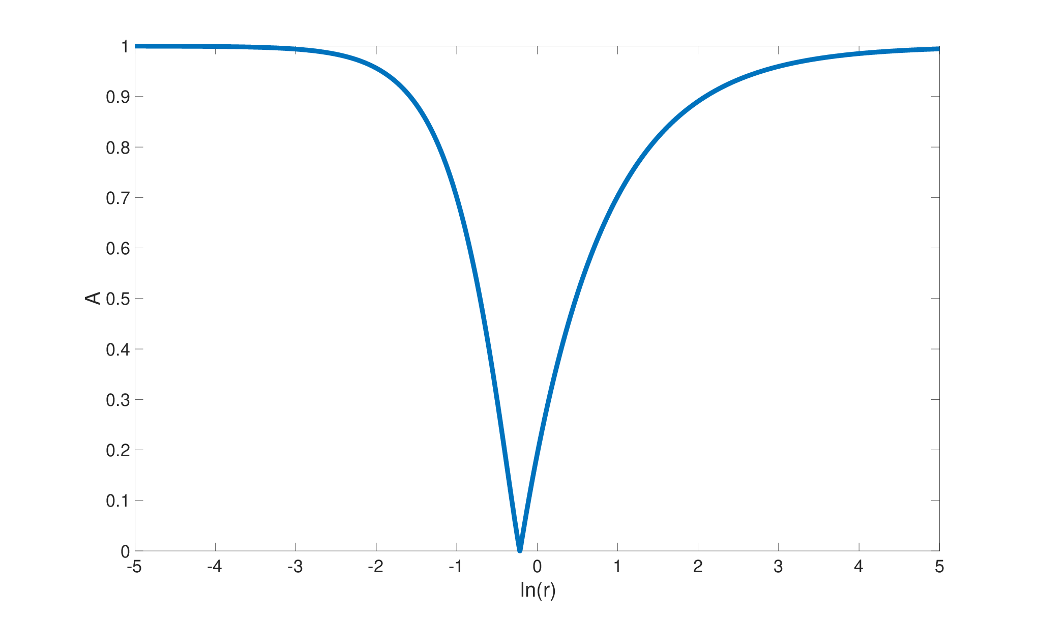
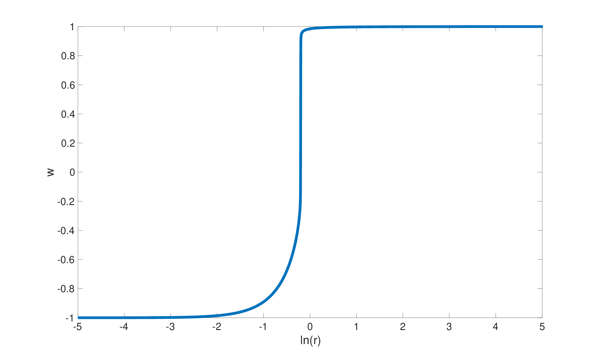
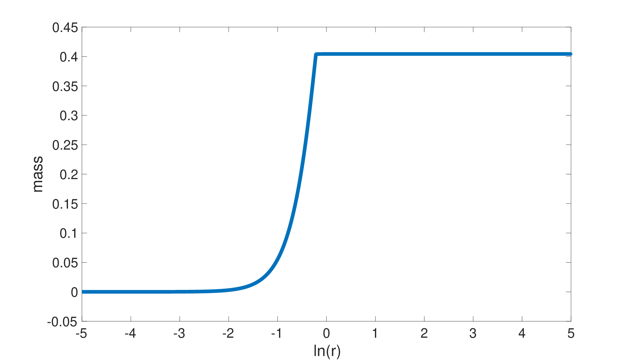
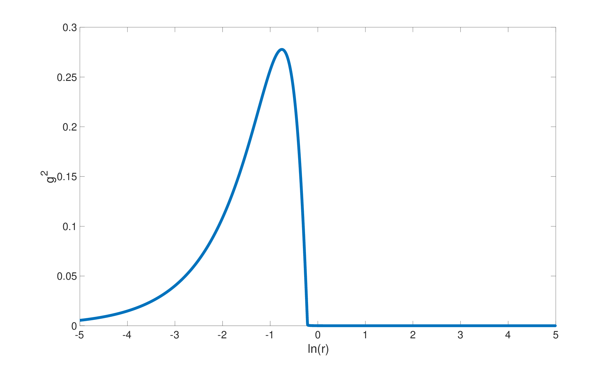
We compute the $L^{\infty}$ and $L_{1}$ errors and orders in Table 1. Since we do not know the exact solution of EYM equations, as a substitution we use numerical solutions obtained on a fine grid with $2^{15}$ points as approximations to the exact solutions, which are denoted by $W_{15}$ and $A_{15}$. This table show that our numerical scheme converge to the right solution with sixth-order. The mass is defined by

$$m=\frac{r}{2}(1-A).$$

We plot the mass in Fig. 1.

The mass function $m(r)$ increase to the total mass $M=0.40.$ Bizon’s solution is quite similar to the Resissner-Nordstrom solution near to the event horizon2. In order to compare with Bizon’s cloled black hole, we define the RN (magnetic) charge as Bartink

$$g^{2}(r)=2r(M-m).$$

Fig. 1 indicates that $g^{2}$ is approximately 0.3 near the horizon. However, Bizon’s colored black hole have the charge $g^{2}\approx 1$ close to horizon2. In the far-field region, $W\to 1$ and the YM charge disappear. The ADM mass is the sole global parameter used to describe the metric at infinity. The Schwarzschild solution must therefore be the only black hole solution, in accordance with the no-hair conjecture.

Separation of variables

	$\displaystyle\tilde{W}(t,r)$	$\displaystyle=\xi(r)e^{i\sigma t},$		(18)
	$\displaystyle\tilde{A}(t,r)$	$\displaystyle=\alpha(r)e^{i\sigma t},$		(19)
	$\displaystyle\tilde{\delta}(t,r)$	$\displaystyle=\beta(r)e^{i\sigma t}.$		(20)

We reduce the following ODE eigenvalue problem

	$\displaystyle p(x)\xi\sigma^{2}$	$\displaystyle=-\xi_{xx}g_{1}(x)^{2}+\Omega_{1}(x)\xi_{x}+\Omega_{2}(x)\xi,$		(21)
	$\displaystyle\xi(-5)$	$\displaystyle=0,~\xi(5)=0.$		(22)

where $p(x),\Omega_{1},\Omega_{2},g_{1}$ are defined in supplemental material. We use the second order center finite difference scheme to approximate (21):

	$\displaystyle p_{j}\xi_{j}\sigma^{2}=-\frac{g_{1}(x_{j})^{2}}{h^{2}}(\xi_{j+1}-2\xi_{j}+\xi_{j-1})+$
	$\displaystyle\Omega_{1}(x_{j})\frac{1}{2h}(\xi_{j+1}-\xi_{j-1})+\Omega_{2}(x_{j})\xi_{j}$		(23)

for $j=1,..n$ with the following boundary conditions

	$\displaystyle\xi_{0}$	$\displaystyle=0,$		(24)
	$\displaystyle\xi_{n+1}$	$\displaystyle=0.$		(25)

Then we obtain an algebraic eigenvalue problem which can be written as

$\displaystyle\Lambda\Xi=\sigma^{2}P\Xi,$

(26)

where $\Lambda$ is a tridiagonal matrix, $\Xi$ is the vector with components $\xi_{j}$ and $P$ is a diagonal matrix whose $j$th element is $p_{j}$. We now find the eigenvalues by using a standard matrix technique such as the Rayleigh quotient iteration and QR Algorithm. The first eigenvalue with is

$$\min(\sigma^{2})=462.04855,$$

which means $\sigma$ is a real number. Substituting this value into (18)-(20), we can see that the amplitude of the perturbation will not grow. But we still need a strong evidence that the perturbation will decay. Hence, we consider the nonlinear perturbation of the static solution in the next section.

Nonlinear perturbation.—The EYM equation can be written as

	$\displaystyle r^{2}e^{\delta}(\frac{e^{\delta}}{A}W_{t})_{t}$	$\displaystyle=AW_{xx}+(1-2A-\frac{(1-W^{2})^{2}}{r^{2}})W_{x}$
		$\displaystyle~~~+(1-W^{2})W,$		(27)
	$\displaystyle A_{x}$	$\displaystyle=-(1+\Pi^{2}+\Phi^{2})A+1-\frac{(1-W^{2})^{2}}{r^{2}},$		(28)
	$\displaystyle\delta_{x}$	$\displaystyle=-(\Pi^{2}+\Phi^{2}),$		(29)

where

$\displaystyle\Pi$

$\displaystyle=\frac{e^{\delta}}{A}W_{t},~\Phi=\frac{\sqrt{2}W_{x}}{r}.$

(30)

We give the initial perturbations as:

	$\displaystyle\text{data 1}:W(0,x)$	$\displaystyle=W_{0}(x)+0.1e^{-50(x-3)^{2}},W_{t}(0,x)=0,$		(31)
	$\displaystyle\text{ data 2}:W(0,x)$	$\displaystyle=W_{0}(x)+0.1e^{-50(x+3)^{2}},W_{t}(0,x)=0.$		(32)

where $W_{0}(x)$ is static solution. We introduce auxiliary variables $\alpha$ and $\beta$ defined as below and thus can rewrite the EYM equations as

	$\displaystyle c$	$\displaystyle=2A-1+\frac{(W^{2}-1)^{2}}{r^{2}},$		(33)
	$\displaystyle\alpha$	$\displaystyle=\frac{e^{2\delta}r^{2}}{A},$		(34)
	$\displaystyle\beta$	$\displaystyle=r^{2}e^{\delta}(\frac{e^{\delta}}{A})_{t},$		(35)
	$\displaystyle\alpha W_{tt}+\beta W_{t}$	$\displaystyle=AW_{xx}-cW_{x}+(1-W^{2})W,$		(36)
	$\displaystyle A_{x}$	$\displaystyle=-(1+\Pi^{2}+\Phi^{2})A+1-\frac{(1-W^{2})^{2}}{r^{2}},$		(37)
	$\displaystyle\delta_{x}$	$\displaystyle=-(\Pi^{2}+\Phi^{2}).$		(38)

One can find the numerical detail in Chapter 4 of supplemental material. Next, we define $\Delta W(t,x)=W(t,x)-W_{0}(x)$ and compute the evolution of $\Delta W(t,x)$.
Based on the numerical evidence, we speculate that the static solution $W(x,t)$ is stable in the $BV$ norm. More precisely, we conjecture that $\|\Delta W\|_{BV}\to 0$ as $t\to\infty$.

As shown in Fig.2, both the $L^{\infty}$ norm and the $BV$ norm of $\Delta W$ decay to 0 as the time increases. Therefore, the perturbation solution converges to the steady state solution $W_{0}$, which indicates that our solution $W_{0}$ is nonlinearly stable.

Geometry and light cones in EYM spacetime — The Riemann curvature of EYM spacetime are regular at $r=0$ (i.e., $x=-\infty$), but are singular at $x=-0.21$,furthermore, the Kretschmann scalar and Ricci scalar also blow up at the horizon but keep regular at $r=0$,which are different from Schwarzschild spacetime. The light cone structure shows that there is an apparent horizon at $x=-0.21$. For more detail, such as the null geodesics, the time-like geodesic and the space-time diagram in Eddington-Finkelstein coordinates. One can find in Chapter 5 of supplemental material.

Conclusion and Discussion— In this paper, we give strong evidence of stability of our solution. In the future, rigorous analytical proof will be given. We shall also study more general metric where the tensor will have more mixed terms. On the physical side, the stability of the solutions suggests that, in early universe when gauge field plays a dominant role in the evolution, the coupling of gravity and gauge field would generate a new type of stable black holes. These primordial black holes left over from early Universe might be a source of dark matter at the present epoch dm; bcm.

References

- (1) R. Bartnik and J. McKinnon, Particle-like solutions of the Einstein Yang-Mills equations, Phys. Rev. Lett. 61, 141 (1988).
- (2) P. Bizon, Colored black holes, Phys. Rev. Lett. 64, 2844 (1990).
- (3) M. S. Volkov and D. V. Gal’tsov, NonAbelian Einstein-Yang-Mills black holes, Sov. J. Nucl. Phys. 51, 1171 (1990).
- (4) H. P. Künzle and A. K. M. Masood-ul-Alam, Spherically symmetric static Einstein-Yang-Mills fields, J. Math. Phys. 31, 928 (1990).
- (5) M. W. Choptuik, J. Chmaj, and P. Bizoń, Critical Behavior in Gravitational Collapse of a Yang-Mills Field, Phys. Rev. Lett. 773, 424-427 (1996).
- (6) M. Maliborski and O. Rinne, Critical phenomena in the general spherically symmetric Einstein-Yang-Mills system, Phys. Rev. D 97, 044053 (2018).
- (7) M. W. Choptuik, E. W. Hirschmann, and R. L. Marsa. New Critical Behavior in Einstein-Yang-Mills Collapse, Phys. Rev. D 60, 124011 (1999).
- (8) O. Rinne, Formation and decay of Einstein-Yang-Mills black holes, Phys. Rev. D 90, 124084 (2014).
- (9) A. Zenginolu, A hyperboloidal study of tail decay rates for scalar and Yang-Mills fields, Class. Quantum Grav. 25, 175013 (2008).
- (10) M. Pürrer and P. C. Aichelburg, Tails for the Einstein-Yang-Mills system, Class. Quantum Grav. 26, 035004 (2009).
- (11) P. Bizoń, A. Rostworowski, and A. Zenginoulu, Saddle-point dynamics of a Yang-Mills field on the exterior Schwarzschild spacetime, Class. Quantum Grav. 27, 175003 (2010).
- (12) J. A. Smoller, A. G. Wasserman, S.-T. Yau, and J. B. McLeod, Smooth static solutions of the Einstein-Yang/Mills equation, Commun. Math. Phys. 143, 115-147 (1991).
- (13) J. A. Smoller, A. G. Wasserman, and S.-T. Yau, Existence of black-hole solutions for the Einstein-Yang/Mills equations, Commun. Math. Phys. 154, 377-401 (1993).
- (14) J. A. Smoller, A. G. Wasserman, Existence of infinitely-many smooth, static, global solutions of the Einstein/Yang-Mills equations, Commun. Math. Phys. 151, 303-325 (1993).
- (15) J. A. Smoller and A. G. Wasserman, Reissner-Nordström-like solutions of the spherically symmetric Einstein/Yang-Mills equations, J. Math. Phys. 38, 6522-6559 (1997).
- (16) J. A. Smoller and A. Wasserman, Regular solutions of the Einstein-Yang-Mills equations, J. Math. Phys. 36, 4301-4323 (1995).
- (17) N. Straumann and Z. H. Zhou, Instability of the Bartnik-mckinnon solution of the Einstein-Yang-Mills Equations, Phys. Lett. B 237, 353-356 (1990).
- (18) N. Straumann and Z. H. Zhou, Instability of a colored black hole solution, Phys. Lett. B 243, 33-35 (1990).
- (19) P. Bizon and R. M. Wald, The colored black hole is unstable, Phys. Lett. B 267, 173-174 (1991).
- (20) Z. H. Zhou and N. Straumann, Nonlinear perturbations of Einstein-Yang-Mills solitons and non-abelian black holes, Nucl. Phys. B 360, 180-196 (1991).
- (21) Y. Liu, C.-W Shu, and M. Zhang, High order finite difference WENO schemes for nonlinear degenerate parabolic equations, SIAM J. Sci. Comput. 33 (2), 939–965 (2011).
- (22) C.-W. Shu, Essentially non-oscillatory and weighted essentially non-oscillatory schemes for hyperbolic conservation laws, in Advanced Numerical Approximation of Nonlinear Hyperbolic Equations. B. Cockburn, C. Johnson, C.-W. Shu, and E. Tadmor (Editor: A. Quarteroni), Lecture Notes in Mathematics, volume 1697, Springer, pp. 325-432 (1998).
- (23) B. Carr and F. Kühnel, Primordial Black Holes as Dark Matter: Recent Developments, Annu. Rev. Nucl. Part. Sci. 70, 355–394 (2020).
- (24) S. Bird, I. Cholis, J. B. Muñoz, Y. Ali-Haïmoud, M. Kamionkowski, E. D. Kovetz, A. Raccanelli, and A. G. Riess, Did LIGO Detect Dark Matter? Phys. Rev. Lett. 116, 201301 (2016).