Capture of a diffusing lamb by a diffusing lion when both return home
Abstract
A diffusing lion pursues a diffusing lamb when both of them are allowed to get back to their homes intermittently. Identifying the system with a pair of vicious random walkers, we study their dynamics under Poissonian and sharp resetting. In absence of any resets, the location of intersection of the two walkers follows a Cauchy distribution. In presence of resetting, the distribution of the location of annihilation is composed of two parts: one in which the trajectories cross without being reset (center) and the other where trajectories are reset at least once before they cross each other (tails). We find that the tail part decays exponentially for both the resetting protocols. The central part of the distribution, on the other hand, depends on the nature of the restart protocol, with Cauchy for Poisson resetting and Gaussian for sharp resetting. We find good agreement of the analytical results with numerical calculations.
I Introduction
Search is a fundamental endeavor to survival ranging from human search Bell 2012 to rescue operations Shlesinger 2009 to animal foraging Bartumeus and Catalan 2009; Bénichou et al. 2006 to protein binding on DNA Coppey et al. 2004, transcription factors searching for a specific DNA von Hippel 2007; Gorman and Greene 2008, to mention a few. A useful search strategy involves intermittent phases of slow motion aiding the searcher in target detection and fast motion allowing the searcher to cover maximal ground in minimal time Bénichou et al. 2011. Restarting a search process at intermittent intervals, aka stochastic resetting, has been extensively shown to expedite search Evans et al. 2020. Stochastic resetting has been a very active topic of research within the realm of nonequilibrium statistical physics over the past decade Evans et al. 2020. The basic essence of stochastic resetting is that in any kind of search process, the search is rarely successful in the first attempt. Following which the search is restarted again and again until the process culminates with success. This property is common to a wide variety of search processes. Now it is almost always true that if sufficient amount of time is devoted, then any search shall meet success. The question of value is, however, whether an intermittent restart of the search process tends to reduce the time of completion? Answer to this question is affirmative. At least in the case of stochastic algorithms it has been shown that a simple restart might expedite completion Luby et al. 1993; Tong et al. 2008; Avrachenkov et al. 2013. Not only in endeavors of human interest, nature also employs restarts in many processes, for example enzymatic reactions following the Michaelis-Menten reaction scheme Michaelis and Menten 1913.
The idea of stochastic resetting to Brownian search problem was first applied in the seminal work of Evans and Majumdar Evans and Majumdar 2011a. They showed that restarting a Brownian particle to its initial location at a constant rate renders the mean first passage time (MFPT) finite. The process of restarting a stochastic process at a constant rate is termed as Poissonian resetting. In addition to Brownian motion, Poissonian resetting has been applied to run and tumble particles Evans and Majumdar 2018, fluctuating interfaces Gupta et al. 2014, dynamical phase transitions Majumdar et al. 2015; Singh et al. 2022, resetting transitions Ahmad et al. 2019; Ahmad et al. 2022, telegraphic processes Masoliver 2019, comb-like structures Domazetoski et al. 2020; Singh et al. 2021, multiple Brownian searchers Evans and Majumdar 2014, etc. However, Poissonian resetting is not exclusive and other protocols like power-law distributed resetting times Nagar and Gupta 2016, resetting rates depending on space Evans and Majumdar 2011b and time Pal et al. 2016 have also been extensively studied. This raises an interesting question: given the wide class of resetting protocols, does there exist a reset mechanism under which MFPT is minimal? This question is difficult to answer in its full generality. However, when resetting is renewal, then sharp resetting in which the time interval between two resets is fixed serves as the best strategy Pal and Reuveni 2017; Chechkin and Sokolov 2018. In other words, “if there exists a stochastic resetting protocol that improves search process, then there exists a deterministic restart protocol that performs as good or better” Eliazar and Reuveni 2020.
Poissonian and sharp restarts lie at the two extremes of renewal resetting, former being memoryless and the latter retaining its entire memory. Both these protocols were compared against each other for a system of Brownian particles searching for a target in Ref. Bhat et al. 2016 and it was shown that sharp resetting typically leads to a lower search cost than that in Poissonian resetting. This study was taken further for a system of Brownian particles where interactions are relevant, for example, in population genetics da Silva and Fragoso 2021. Inclusion of interactions further allows to consider more nontrivial forms of resetting mechanisms such as those which are driven by the interactions between the constituent particles Falcao and Evans 2017 or space dependent resetting in interacting Brownian particles Bertin 2022. One of the most important examples which involves interacting random walks is the well known prey predator model which culminates when the prey is captured by the predator Krapivsky and Redner 1996. An exactly solvable prey predator model with resetting was recently considered by Evans and co-workers Evans et al. 2022 where the prey on its encounter with a predator can either perish or be reset to its initial location.
In the present work we consider the prey predator model within the realm of vicious random walks which annihilate each other the moment their trajectories cross Bray et al. 2013. The concept was first introduced by Fisher in the context of interfacial wetting in 1+1 dimensions Fisher 1984; Huse and Fisher 1984 and has since been applied to Coulomb gas Forrester 1989 and random matrices Baik 2000. The survival probability for vicious random walkers in one dimension exhibits power law decaying tails Bray and Winkler 2004, and any two such walkers shall certainly meet each other as a random walk in one dimension is recurrent Klafter and Sokolov 2011; Weiss and Rubin 1983. The problem of reunion of two vicious random walks corresponds to the following chemical reaction: Cardy and Täuber 1996 and is one of the most classic problems in nonequilibrium statistical physics Fisher and Gelfand 1988; Schehr et al. 2008; Kundu et al. 2014. The annihilating nature of the vicious walkers makes them suitable for studying directed polymer brushes wherein the viciousness captures the role of the non-intersecting property of polymers Essam and Guttmann 1995. Vicious random walks have also been applied to breathing DNA with the collapse of the bubbles viewed as an annihilation of two vicious walkers moving in opposite potentials Pedersen et al. 2009. Furthermore, the distribution of the location of coalescence makes it relevant to study the location where the trajectories of two vicious walkers cross. In the context of the capture problem where a hungry lion pursues a lamb Redner and Krapivsky 1999, the location of intersection tells us how far the hunt is made from the home. The scenario also makes the concept of resetting very natural Reuveni 2016. This is because either the lamb shall every now and then return to its home, or the lion to its den, or both. The reason that such a thing might happen as the lion pursues the lamb but could not catch it and gets tired eventually getting back in its cave. On the other hand, the freely roaming lamb might spot the lion and run away from it. This makes the study of vicious random walks under resetting very natural. In other words, if we have two vicious Brownian particles we want to know how long do they survive without crossing each other’s paths? And if their trajectories cross, what is the nature of the distribution of such a point? Do the answers to these questions depend on the resetting protocol employed? We address these questions in the following sections by studying the system of two vicious Brownian particles under resetting. The particles are reset identically to their respective initial positions either at constant rates (Poissonian resetting) or after fixed time intervals (sharp resetting).
II Two vicious random walkers
Consider two Brownian particles:
| (1a) | ||||
| (1b) | ||||
where are independent Gaussian random deviates with mean zero and delta correlated variance, that is, and . At the two walkers are at and . The two walkers annihilate each other as soon as their paths cross, that is, . The problem is readily transformed to the motion of the center of mass and relative separation of the two particles . In terms of the new coordinates, the center of mass moves as a free Brownian particle as
| (2) |
where and with . On the other hand, the relative coordinate moves like a Brownian particle on line
| (3) |
where and with . Before the trajectories of the two particles cross, the center of mass exhibits a Brownian motion centered at with a diffusion coefficient and the relative coordinate is a Brownian particle starting at with an absorbing wall at . The first passage time distribution (FPTD) of the relative coordinate to the absorbing wall at is and the probability density function (PDF) of the center of mass motion is Gardiner 1985; Redner 2001. From the FPTD it is evident that the mean time to the annihilation of the two vicious walkers is infinite. The recurrence of a Brownian motion in one dimension, however, implies that the two walkers will eventually collide, and the PDF of the location of intersection is
| (4) |
which is a Cauchy distribution centered at . Similar to the MFPT, there is no well defined mean location of the intersection of the two vicious walkers. This is because even though the two walkers shall certainly meet, they may take really long time to do so by venturing out in opposite directions resulting in the divergence of MFPT and a well defined mean location of annihilation. In other words, the hungry lion may keep pursuing the lamb forever and might eventually die of hunger. And this is where resetting comes in to prevent the hungry lion from dying.
III Resetting to initial configuration
With the vector defining the system, define a resetting protocol: after an interval of reset time the system is reverted back to its initial configuration. The time is either an exponentially distributed random variable (Poissonian resetting) or a fixed quantity (sharp resetting). For simplicity let us assume that the two walkers are reset via identical resetting protocols at exact same time. The reason for this choice is the following: let us assume that the two walkers are reset at different times and , then a scenario is possible in which and just before reset has taken place. The moment after the reset we have which apparently means that the two trajectories have crossed paths. Such crossing of two walkers is, however, erroneous as at the time of reset the first particle is removed from its current location and put back to its initial location instantaneously. This makes intersection point an ill-defined quantity simply for the reason that actual trajectories did not cross. We avoid such a pathological situation by requiring that the two particles be reset at exact same time. Furthermore, restarting the two walkers identically retains the advantage that the two particle system is still described by the motion of the center of mass and motion about the center of mass. Next we consider the two resetting protocols one by one.
III.1 Poissonian resetting
Let the two walkers be reset to their respective initial locations at a rate . Then the FPTD of the relative coordinate under Poissonian resetting is Reuveni 2016
| (5) |
where is the Laplace transform of the FPTD without resetting Oberhettinger and Badii 2012. From this follows the MFPT under Poissonian resetting as: . This result has been previously derived in Evans and Majumdar 2011a via the backward Fokker-Planck equation and many works following it. Here we state the result as a reminder that MFPT under Poissonian resetting is finite.
In order to study the effect of resetting on the PDF of intersection of the two trajectories, we need the FPTD given in terms of the Bromwich integral Arfken and Weber 1999
| (6) |
where and . This integral is easily evaluated from the residue of at the pole closest to . The pole of is given by the solution of which in terms of reads Evans and Majumdar 2011a
| (7) |
and has a unique nonzero solution . Thus, the FPTD at large times is Evans and Majumdar 2011a
| (8) |
where implying that at large times the FPTD under resetting possesses exponentially decaying tails. This result is verified numerically and a good agreement is found for the characteristic decay exponent as shown in Fig. 1(a).


Next, we estimate the PDF of the center of mass motion under resetting, following the renewal equation Evans et al. 2020
| (9) |
where the first term gives the contribution from the trajectories which have not been reset at all, while the second term describes the effect of resetting. As a result, the PDF of the intersection point of the two vicious walkers under Poissonian resetting annihilating each other with FPTD is
| (10) |
where denotes the single integral and denotes the double integral. In what follows we shall see that having the contribution of intersection points without reset captures the central part of the PDF . While describes the tails consisting the intersection points with reset, hence the usage of the superscripts and respectively. Let us now proceed to evaluate the two integrals in (III.1) one by one.
For the single integral in Eq. (III.1), , since the system behaves like the one without resetting. Furthermore, if we look at the FPTD under Poissonian resetting, that is, , then at small times , which is exactly the same quantity as appearing in the first integral in (III.1). In other words, the probability of crossing of two trajectories without being reset is , effectively modifying the FPTD entering in the evaluation of . Hence, we have
| (11) |
where is the modified Bessel function of the second kind and it enters while evaluating the Laplace transform of Oberhettinger and Badii 2012. The double integral in (III.1) is similarly evaluated
| (12) |
where and . Combining the results in (III.1) and (III.1) we have
| (13) |
From Eq. (13), it is evident that describes the center and the tails of the PDF . This is due to the rapid decay of the modified Bessel function as compared to exponential. Furthermore, for small arguments decays algebraically, that is, Abramowitz et al. 1988, from where it follows that behaves like a Cauchy distribution. Thus, when the two walkers are reset to their initial locations at a constant rate, the PDF exhibits a Cauchy distributed center and exponentially decaying tails. In other words, Poissonian resetting of the two walkers reduces the fat tails of the PDF to the center and the far tails are modified to exponential. In summary,
| (14) |
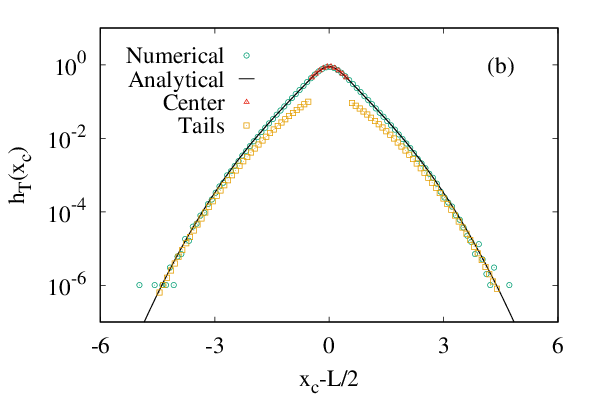
We compare the analytically estimated PDF in Eq. (13) (black solid line) with numerical calculations (green circles) in Fig. 1(b) and find that they are in close proximity.
The contribution to the PDF coming from in the range is scaled by a factor to match the numerically estimated . The reason for doing this is to show that indeed captures the shape of the center of the PDF. The tail part in region matches well with numerically estimated as following the similar decay rate as shown in Fig. 1(b). Here, we refer to the region as the central part. The simple reason for the usage of this terminology is that the center of mass is midway between the two vicious particles and an annihilation taking place within this region would simply mean that the center of mass has not ventured far from its mean position.
III.2 Sharp resetting
In sharp resetting, the two walkers are reset to their respective initial locations after fixed intervals of time . In order to estimate the FPTD under sharp resetting, we use the results derived by Pal and Reuveni in Ref. Pal and Reuveni 2017. They show that if is the time of completion of a stochastic process without restart, and is the time interval of restart, then the FPTD under restart reads Pal and Reuveni 2017
| (15) |
where is the random restart time given restart occurred before completion and is the random completion time without any restarts. For Poissonian resetting when is an exponentially distributed random variable, that is, , Eq. (15) reduces to (5) (see SM in Ref. Pal and Reuveni 2017). For sharp resetting at fixed intervals of time , the distribution of restart times is . As a result,
| (16) |
The integral in the third line does not contribute anything as the limits of integration do not contain the point . In a similar manner
| (17) |
Using (III.2) and (17) in Eq. (15) we find that the FPTD of a stochastic process under sharp restart is given by
| (18) |
where is the FPTD without restart and the subscript on the lhs denotes the time of sharp restart . From the FPTD in (18) follows the MFPT under sharp restart
| (19) |
which has been earlier derived in Ref. Eliazar and Reuveni 2020 in an alternative manner with denoting the survival probability.
For the system of two vicious random walkers Redner 2001. Using these in (19) we have the MFPT to annihilation under sharp resetting
| (20) |
The integral of above has been evaluated using the integral representation of the error function and related Laplace transforms Oberhettinger and Badii 2012; Gradshteyn and Ryzhik 2014. Once again it is evident that resetting gives a finite MFPT. Next we look at the PDF of the intersection point.
In order to evaluate the PDF of the intersection point under sharp resetting, we need the time domain representation of FPTD in Eq. (18). Using we have
| (21) |
where we have used the approximation in the limit of large times (small behavior). The integral is now straightforwardly evaluated from the pole in the complex plane located at . As a result
| (22) |
which implies that at large times decays exponentially as , since . We numerically estimate the characteristic decay time in Fig. 2(a) and find good agreement with the analytical result.

Now we estimate the PDF of the center of mass under sharp resetting. When the two vicious walkers are reset to their initial locations regularly after interval , the number of renewals taking place upto time equals ( denotes the floor function). Furthermore, since the center of mass starts afresh after every reset, its PDF at time is given by
| (23) |
For we have and the center of mass evolves with the PDF . If the trajectories of the two walkers cross before any restart, then the time of their annihilation follows the FPTD . As a result, similar to the case of Poissonian resetting, the PDF of the intersection point is composed of two parts: one coming from the trajectories which annihilate each other at , and the remaining ones which undergo at least one reset event before crossing their paths. Thus, the PDF of the intersection point under sharp resetting is
| (24) |
where and denote the integrals in the intervals and respectively and are defined analogous to their Poissonian counterparts. The first integral is relatively straightforward and evaluates to
| (25) |
This implies that under sharp resetting the fat tails of the Cauchy distribution are tamed to an effective Gaussian. It becomes even more interesting once we realize that here we are considering those trajectories which have not even reset once. In other words, the fact that a restart is set to take place at , forces a certain fraction of trajectories to cross their paths, thus introducing Gaussian cutoffs in the tails. In addition, the central part of the PDF close to the initial location of the center of mass is Gaussian. Now coming to the second integral in (III.2), we have
| (26) |
where the limits of integration are kept from to for reasons stated above. The integral in (III.2) can be evaluated by decomposing the interval of integration into subintervals of length . This helps us to reduce the integral on the real line to an integration over the interval . The reason we can do this is that the floor function turns into a periodic function. As a result
| (27) |
where and the integral is evaluated using MAXIMA. This implies that the PDF of the intersection point has exponentially decaying tails for large . Using (III.2) in (III.2) and then along with (III.2) in Eq. (III.2) we have
| (28) |
We numerically study the PDF of the intersection point in Fig. 2(b) and find that Eq. (III.2) agrees well with numerical calculations. Furthermore, the PDFs (with a scale factor ) and also individually agree with the numerically estimated in their respective ranges (as stated above in case of Poissonian resetting). While it may not be apparent from Fig. 2 (b), the tails of are indeed exponential. This follows from the fact that in Eq. (III.2) the second erfc term describing the tails approaches a constant for large fluctuations, while the third term approaches zero. As a consequence, for large .
IV Comparing Poisson resetting and sharp resetting


So far we have studied the dynamics of two vicious walkers under Poissonian and sharp resetting, but in separate scenarios. It thus becomes interesting to comparing the two protocols against each other. Answer to this question is known partly in that sharp resetting wins over Poissonian resetting in renewal resetting scenario Pal and Reuveni 2017. Hence we compare the minima of the MFPTs under the two resetting protocols. For this purpose let us choose and . As a result we have
| (29a) | ||||
| (29b) | ||||
From the above equations, the minima of the MFPT occurs at where . For this value of the resetting rate . Similarly, has a global minima at which implies . To get a perspective of these numbers, the diffusive time scale of the relative coordinate to cover a distance is for . On this time scale, the MFPT for the two vicious walkers to annihilate each other is . Furthermore, the relative advantage of sharp resetting over Poissonian resetting is which is significant. In other words, while it is suitable for the lion to quickly hunt that both the lion and the lamb return to their homes after fixed time intervals, for the lamb Poissonian resetting is better as it might survive a little longer. We compare the two resetting protocols graphically in Fig. 3(a) and see the relative advantage of sharp resetting over Poisson resetting.
Let us now look at the tail behavior of the PDF of the intersection point for Poisson and sharp resetting at their optimal levels respectively. From Eq. (III.1) it is clear that for Poissonian resetting . On the other hand, for sharp resetting we have . As a result, the tail part of the PDF of the location of intersection is . This implies that at optimal resetting, the tails of the PDF decay faster for sharp resetting as compared to Poissonian resetting. This also follows from the fact that at optimal resetting , as a result both the lion and the lamb do not venture far from their homes at the time of capture under sharp resetting as compared to Poissonian resetting. We compare the two PDFs both numerically and analytically in Fig. 3 (b) and find the PDF for Poissonian resetting has a higher spread as compared to that for sharp resetting.
V Conclusions
In the realm of nonequilibrium statistical physics vicious random walkers are used to model interfacial wetting in dimensions and non-intersecting polymers. In these contexts the survival probability and the distribution of the location of coalescence are relevant quantities to address. Within the domain of capture problems, vicious random walks translate to the capture of a prey by a predator. Motivated by these examples, in this paper we study the annihilation properties of two vicious random walkers under Poissonian and sharp resetting protocols. In absence of resetting the mean time of capture is divergent while the location of annihilation follows a Cauchy distribution. Introduction of resetting in the system renders finite MFPT due to the fact that the FPTD tails now decay exponentially as compared to algebraically in absence of resetting. Furthermore, tails of the PDF of annihilation location now decay exponentially. This is independent of the exact nature of resetting protocol. The central part of the PDF, however, depends on the way system is reset to its initial location. For Poissonian resetting the central part of the PDF is a Cauchy distribution, while for sharp resetting it is a Gaussian.
We have reset the two walkers identically so that we can reduce the two particle system as to be described by the motion of the center of mass and motion about the center of mass. We have also assumed that restarts are instantaneous, but in any realistic scenario bringing back the system to its initial state takes a finite amount of time. Even within the realm of instantaneous resetting, we chose the particles to be identical. What would happen if we include inertia and assign different masses to different particles? We explore these and other interesting possibilities in future works.
Acknowledgments: RKS thanks the Israel Academy of Sciences and Humanities (IASH) and the Council of Higher Education (CHE) Fellowship. SS acknowledges the HPC facility at Ben-Gurion University.
References
- Bell (2012) W. J. Bell, Searching behaviour: the behavioural ecology of finding resources (Springer Science & Business Media, 2012).
- Shlesinger (2009) M. F. Shlesinger, J. Phys. A: Math. Theor. 42, 434001 (2009).
- Bartumeus and Catalan (2009) F. Bartumeus and J. Catalan, J. Phys. A: Math. Theor. 42, 434002 (2009).
- Bénichou et al. (2006) O. Bénichou, C. Loverdo, M. Moreau, and R. Voituriez, Phys. Rev. E 74, 020102 (2006).
- Coppey et al. (2004) M. Coppey, O. Bénichou, R. Voituriez, and M. Moreau, Biophys. J. 87, 1640 (2004).
- von Hippel (2007) P. H. von Hippel, Annual Rev. Biophys. Biomol. Struct. 36, 79 (2007).
- Gorman and Greene (2008) J. Gorman and E. C. Greene, Nature Struct. & Mol. Bio. 15, 768 (2008).
- Bénichou et al. (2011) O. Bénichou, C. Loverdo, M. Moreau, and R. Voituriez, Rev. Mod. Phys. 83, 81 (2011).
- Evans et al. (2020) M. R. Evans, S. N. Majumdar, and G. Schehr, J. Phys. A: Math. Theor. 53, 193001 (2020).
- Luby et al. (1993) M. Luby, A. Sinclair, and D. Zuckerman, Information Processing Lett. 47, 173 (1993).
- Tong et al. (2008) H. Tong, C. Faloutsos, and J.-Y. Pan, Knowledge and Information Systems 14, 327 (2008).
- Avrachenkov et al. (2013) K. Avrachenkov, A. Piunovskiy, and Y. Zhang, J. Appl. Prob. 50, 960 (2013).
- Michaelis and Menten (1913) L. Michaelis and M. L. Menten, Biochem. z 49, 352 (1913).
- Evans and Majumdar (2011a) M. R. Evans and S. N. Majumdar, Phys. Rev. Lett. 106, 160601 (2011a).
- Evans and Majumdar (2018) M. R. Evans and S. N. Majumdar, J. Phys. A: Math. Theor. 51, 475003 (2018).
- Gupta et al. (2014) S. Gupta, S. N. Majumdar, and G. Schehr, Phys. Rev. Lett. 112, 220601 (2014).
- Majumdar et al. (2015) S. N. Majumdar, S. Sabhapandit, and G. Schehr, Phys. Rev. E 91, 052131 (2015).
- Singh et al. (2022) R. K. Singh, K. Gorska, and T. Sandev, Phys. Rev. E 105, 064133 (2022).
- Ahmad et al. (2019) S. Ahmad, I. Nayak, A. Bansal, A. Nandi, and D. Das, Phys. Rev. E 99, 022130 (2019).
- Ahmad et al. (2022) S. Ahmad, K. Rijal, and D. Das, Phys. Rev. E 105, 044134 (2022).
- Masoliver (2019) J. Masoliver, Phys. Rev. E 99, 012121 (2019).
- Domazetoski et al. (2020) V. Domazetoski, A. Masó-Puigdellosas, T. Sandev, V. Méndez, A. Iomin, and L. Kocarev, Phys. Rev. Res. 2, 033027 (2020).
- Singh et al. (2021) R. K. Singh, T. Sandev, A. Iomin, and R. Metzler, J. Phys. A: Math. Theor. 54, 404006 (2021).
- Evans and Majumdar (2014) M. R. Evans and S. N. Majumdar, J. Phys. A: Math. Theor. 47, 285001 (2014).
- Nagar and Gupta (2016) A. Nagar and S. Gupta, Phys. Rev. E 93, 060102 (2016).
- Evans and Majumdar (2011b) M. R. Evans and S. N. Majumdar, J. Phys. A: Math. Theor. 44, 435001 (2011b).
- Pal et al. (2016) A. Pal, A. Kundu, and M. R. Evans, J. Phys. A: Math. Theor. 49, 225001 (2016).
- Pal and Reuveni (2017) A. Pal and S. Reuveni, Phys. Rev. Lett. 118, 030603 (2017).
- Chechkin and Sokolov (2018) A. Chechkin and I. M. Sokolov, Phys. Rev. Lett. 121, 050601 (2018).
- Eliazar and Reuveni (2020) I. Eliazar and S. Reuveni, J. Physics A: Math. Theor. 53, 405004 (2020).
- Bhat et al. (2016) U. Bhat, C. De Bacco, and S. Redner, J. Stat. Mech.: Theor. Exp. 2016, 083401 (2016).
- da Silva and Fragoso (2021) T. T. da Silva and M. D. Fragoso, J. Phys. A: Math. Theor. 55, 014003 (2021).
- Falcao and Evans (2017) R. Falcao and M. R. Evans, J. Stat. Mech.: Theor. Exp. 2017, 023204 (2017).
- Bertin (2022) E. Bertin, arXiv preprint arXiv:2205.00817 (2022).
- Krapivsky and Redner (1996) P. L. Krapivsky and S. Redner, J. Phys. A: Math. Gen. 29, 5347 (1996).
- Evans et al. (2022) M. R. Evans, S. N. Majumdar, and G. Schehr, J. Phys. A: Math. Theor. 55, 274005 (2022).
- Bray et al. (2013) A. J. Bray, S. N. Majumdar, and G. Schehr, Adv. Phys. 62, 225 (2013).
- Fisher (1984) M. E. Fisher, J. Stat. Phys. 34, 667 (1984).
- Huse and Fisher (1984) D. A. Huse and M. E. Fisher, Phys. Rev. B 29, 239 (1984).
- Forrester (1989) P. J. Forrester, J. Stat. Phys. 56, 767 (1989).
- Baik (2000) J. Baik, Commun. Pure Appl. Math.: A Journal Issued by the Courant Institute of Mathematical Sciences 53, 1385 (2000).
- Bray and Winkler (2004) A. J. Bray and K. Winkler, J. Phys. A: Math. Gen. 37, 5493 (2004).
- Klafter and Sokolov (2011) J. Klafter and I. M. Sokolov, First steps in random walks: from tools to applications (OUP Oxford, 2011).
- Weiss and Rubin (1983) G. H. Weiss and R. J. Rubin, Adv. Chem. Phys. 52, 363 (1983).
- Cardy and Täuber (1996) J. Cardy and U. C. Täuber, Phys. Rev. Lett. 77, 4780 (1996).
- Fisher and Gelfand (1988) M. E. Fisher and M. P. Gelfand, J. Stat. Phys. 53, 175 (1988).
- Schehr et al. (2008) G. Schehr, S. N. Majumdar, A. Comtet, and J. Randon-Furling, Phys. Rev. Lett. 101, 150601 (2008).
- Kundu et al. (2014) A. Kundu, S. N. Majumdar, and G. Schehr, J. Stat. Phys. 157, 124 (2014).
- Essam and Guttmann (1995) J. W. Essam and A. J. Guttmann, Phys. Rev. E 52, 5849 (1995).
- Pedersen et al. (2009) J. N. Pedersen, M. S. Hansen, T. Novotnỳ, T. Ambjörnsson, and R. Metzler, J. Chem. Phys. 130, 164117 (2009).
- Redner and Krapivsky (1999) S. Redner and P. L. Krapivsky, Amer. J. Phys. 67, 1277 (1999).
- Reuveni (2016) S. Reuveni, Phys. Rev. Lett. 116, 170601 (2016).
- Gardiner (1985) C. W. Gardiner, Springer series in synergetics 13, 3 (1985).
- Redner (2001) S. Redner, A guide to first-passage processes (Cambridge university press, 2001).
- Oberhettinger and Badii (2012) F. Oberhettinger and L. Badii, Tables of Laplace transforms (Springer Science & Business Media, 2012).
- Arfken and Weber (1999) G. B. Arfken and H. J. Weber, “Mathematical methods for physicists,” (1999).
- Abramowitz et al. (1988) M. Abramowitz, I. A. Stegun, and R. H. Romer, “Handbook of mathematical functions with formulas, graphs, and mathematical tables,” (1988).
- Gradshteyn and Ryzhik (2014) I. S. Gradshteyn and I. M. Ryzhik, Table of integrals, series, and products (Academic press, 2014).