Measurability of neutron star tidal deformability from merging neutron star-black hole binaries
Abstract
The neutron star-black hole binary (NSBH) system has been considered one of the promising detection candidates for ground-based gravitational-wave (GW) detectors such as LIGO and Virgo. The tidal effects of neutron stars (NSs) are imprinted on the GW signals emitted from NSBHs as well as binary neutron stars. The NS tidal deformability () was successfully measured by the binary neutron star signal GW170817 but could not be constrained in the analysis of the two NSBH signals GW200105 and GW200115 due to the low signal-to-noise ratio. In this work, we study how accurately the parameter can be measured in GW parameter estimation for NSBH signals. We set the parameter range for the NSBH sources to for the black hole mass, for the NS mass, and for the dimensionless black hole spin. For realistic populations of sources distributed in different parameter spaces, we calculate the measurement errors of () using the Fisher matrix method. In particular, we perform a single-detector analysis using the advanced LIGO and the Cosmic Explorer detectors and a multi-detector analysis using the 2G (advanced LIGO-Hanford, advanced LIGO-Livingstone, advanced Virgo, and KAGRA) and the 3G (Einstein Telescope and Cosmic Explorer) networks. We show the distribution of for the population of sources as a one-dimensional probability density function. Our result shows that the probability density function curves are similar in shape between advanced LIGO and Cosmic Explorer, but Cosmic Explorer can achieve times better accuracy overall in the measurement of . In the case of the network detectors, the probability density functions are maximum at and for the 2G and the 3G networks, respectively, and the 3G network can achieve times better accuracy overall. Specifically, we investigate the distribution of for Monte Carlo sources in our parameter range with the NS mass fixed to , and the result shows that if the sources are located at , the parameter estimation results for of the sources can distinguish between the theoretical EOS models at the 1– level, using the 3G network. Additionally, we demonstrate that our PDF results are almost unaffected by different choices of the true value of .
I Introduction
Since the first gravitational-wave (GW) signal was detected in 2015 Abbott et al. 2016, the network of the two advanced LIGO (aLIGO) Aasi et al. 2015 and advanced Virgo Acernese et al. 2015 detectors has observed GW candidates Abbott et al. 2019a; Abbott et al. 2021a; Abbott et al. 2021b; Abbott et al. 2021c through three observing runs. All GW signals were emitted from a compact binary coalescence (CBC) system such as binary black hole (BBH), binary neutron star (BNS), and neutron star-black hole binary (NSBH). Most GW sources originated from BBHs, and various BH masses and spins were measured from these signals. The sources of the two signals GW170817 Abbott et al. 2017a; Abbott et al. 2019b and GW190425 Abbott et al. 2020 were identified as BNSs, and GW170817 enabled us to directly measure the NS tidal deformability for the first time through observation means. In particular, since GW170817 had a high signal-to-noise ratio (SNR) , it could be inferred that the soft equation-of-state (EOS) model is preferred over the stiff EOS model Abbott et al. 2019b. In parameter estimation for BNS signals, a well-constrained tidal parameter is the effective tidal deformability rather than the component tidal deformability. The effective tidal deformability is defined by the combination of the masses () and the component tidal parameters (). Since and are generally strongly correlated, their measurement errors can be large even though the effective tidal parameter is well constrained as shown in the result of GW170817 Abbott et al. 2019b.
On the other hand, the two NSBH signals GW200105 and GW200115 were also captured by the LIGO-Virgo network during the third observing run Abbott et al. 2021d (for a brief overview of NSBH mergers, refer to Foucart 2020). Since the GWs from NSBHs also contain an NS tidal effect, information on the tidal parameter can be extracted from those signals. However, the contribution of tidal deformability to the waveform of the NSBH system is relatively small compared to that of the BNS system, especially when the BH mass is much larger than the NS mass. Therefore, a sufficiently high SNR is required to measure the tidal deformability from the NSBH signals. Unfortunately, the observed NSBH signals were not able to constrain the tidal deformability of the NSs well due to their low SNRs. Meanwhile, a large advantage of the NSBH signals when measuring the tidal parameter is that the individual NS tidal deformability rather than the effective tidal deformability can be obtained directly through parameter estimation because the tidal deformability of BH is zero.
The purpose of this work is to investigate how accurately the NS tidal deformability () can be measured from NSBH signals. To this end, we utilize the Fisher matrix method implemented in the python package GWBench Borhanian 2021 and calculate the measurement errors of for realistic populations of NSBH sources. Several parameter estimation studies on the measurability of the NS tidal deformability have been done using Bayesian analysis with stochastic sampling on NSBH systems as well as Fisher Matrix studies. Lackey et al.Lackey et al. 2012 estimated tidal deformability from NSBH systems with nonspinning BHs by applying the Fisher matrix method to the hybrid waveforms based on BBH waveforms calibrated to NSBH numerical simulations, and they extended it to the spinning NSBH systems in subsequent work Lackey et al. 2014. In the former, they showed that for a single aLIGO detector, the tidal parameter can be extracted to accuracy from single events for mass ratios of and at a distance of , and in the latter, for –, BH spins –, NS masses –, and a distance of , a single aLIGO detector can measure to a – uncertainty of –. For both works, they showed that the uncertainty in is an order of magnitude smaller for the 3G detector Einstein Telescope. On the other hand, Kumar et al.Kumar et al. 2017 performed a Bayesian analysis of NSBH systems with spinning BHs to study the measurability of with aLIGO and found that 20–35 events can constrain within –, depending on the EOS.
This paper is organized as follows. In Sec. II, we introduce various waveform models recently developed for use in GW data analysis for BNS or NSBH systems based on the Effective-One-Body (EOB) formalism and the phenomenological fit approach. Next, we give a brief overview of the Bayesian parameter estimation and the Fisher matrix approach in terms of parameter measurement accuracy and list the 2G and the 3G detectors used in our analysis. The results are given in Sec. III. First, we compare the parameter measurement errors obtained from the Fisher matrix approach with those obtained from the Bayesian parameter estimation simulations and verify the reliability of the Fisher matrix method in our analysis. Next, we investigate the suitability of four recent waveform models for applying the Fisher matrix method to NSBH sources in our parameter range and adopt a representative waveform model (denoted by SEOBNR_T in this work). Then, we apply the Fisher matrix method to SEOBNR_T and calculate the measurement errors of for our NSBH sources. We perform a single-detector analysis as well as a multi-detector analysis and provide comparisons between the 2G and the 3G detectors. In particular, using the results for the 3G network, we present a specific example describing how well the theoretical EOS models can be constrained by the NSBH signals. In Sec. IV, we summarize our results and provide some discussion.
II Method
II.1 Waveform models
To simulate an NSBH signal, the waveform model requires the full Inspiral-Merger-Ringdown (IMR) expression, including the NS tidal effect. To date, various IMR waveform models have been developed and implemented in LAL (LIGO Algorithm Library LIGO Scientific Collaboration 2018) for use in GW data analysis. Those models are roughly classified into two waveform families according to the construction formalism. One is based on the Effective-One-Body (EOB) formalism and the other is based on the phenomenological fit approach. In both approaches, the waveform from the late inspiral to the merger-ringdown is calibrated against the aligned-spin BBH NR waveforms. So they are represented by the “SEOBNR” and “IMRPhenom” models.
The EOB formalism is basically constructed in the time domain. For computational efficiency, the frequency-domain model SEOBNRv4_ROM Pürrer 2014; Bohé et al. 2017 has been developed based on the time-domain model SEOBNRv4 using a reduced-order-quadrature rule Smith et al. 2016. SEOBNRv4_ROM_NRTidalv2 builds on SEOBNRv4_ROM by adding tidal correction terms that are constructed from high-resolution BNS NR simulations Dietrich et al. 2017; Dietrich et al. 2019. SEOBNRv4_ROM_NRTidalv2_NSBH Matas et al. 2020 was built from SEOBNRv4_ROM_NRTidalv2 to generate aligned-spin NSBH waveforms by adding corrections to the wave amplitude Pannarale et al. 2015.
Meanwhile, the IMRPhenom models are defined in the frequency domain. Early versions of the IMRPhenom models were developed for the BBH system. IMRPhenomPv2 has been mainly used for CBC analyses in recent years. This model is based on the precessing-spin model IMRPhenomP Hannam et al. 2014 and the aligned-spin model IMRPhenomD Husa et al. 2016; Khan et al. 2016. IMRPhenomPv2_NRTidalv2 is based on IMRPhenomPv2 and includes the same tidal correction terms Dietrich et al. 2017; Dietrich et al. 2019 as in SEOBNRv4_ROM_NRTidalv2. The IMRPhenom family also has an NSBH model IMRPhenomNSBH Thompson et al. 2020. This model is based on the amplitude of IMRPhenomC Santamaría et al. 2010 and the phase of IMRPhenomD Husa et al. 2016; Khan et al. 2016, and incorporates NS tidal effects Dietrich et al. 2019 and amplitude corrections Pannarale et al. 2015 similar to SEOBNRv4_ROM_NRTidalv2_NSBH.
In this work, four recent IMR waveform models containing NS tidal effects are considered, which are listed in Table 1. Finally, we note that the TaylorF2 model also includes NS tidal effects but generates inspiral-only waveforms. TaylorF2 is reliable in parameter estimation for BNS systems such as GW170817 Abbott et al. 2019b and GW100425 Abbott et al. 2020. However, after some consistency tests, we have verified that TaylorF2 is not suitable for the analysis of our NSBH sources.
| Full name (implemented in LAL) | References | |
|---|---|---|
| Short label (used in this work) | Base model | Corrections |
| SEOBNRv4_ROM_NRTidalv2 | Smith et al. 2016; Pürrer 2014; Bohé et al. 2017 | Dietrich et al. 2017; Dietrich et al. 2019 |
| SEOBNR_T | ||
| SEOBNRv4_ROM_NRTidalv2_NSBH Matas et al. 2020 | Smith et al. 2016; Pürrer 2014; Bohé et al. 2017 | Dietrich et al. 2017; Dietrich et al. 2019; Pannarale et al. 2015 |
| SEOBNR_NSBH | ||
| IMRPhenomPv2_NRTidalv2 | Hannam et al. 2014; Husa et al. 2016; Khan et al. 2016 | Dietrich et al. 2017; Dietrich et al. 2019 |
| IMRPhenomP_T | ||
| IMRPhenomNSBH Thompson et al. 2020 | Santamaría et al. 2010; Husa et al. 2016; Khan et al. 2016 | Dietrich et al. 2019; Pannarale et al. 2015 |
| IMRPhenom_NSBH | ||
II.2 Bayesian parameter estimation
The physical properties of the GW source can be measured in the parameter estimation procedure Veitch et al. 2015. This process is based on Bayesian inference statistics, and the algorithm explores the entire parameter space, computing the overlaps between model waveforms and detector data. The result of Bayesian parameter estimation can be given as the posterior probability density functions (PDFs) of the parameters considered. Given the detector data containing the GW signal and noise , the overlap between and the model waveform is defined as
| (1) |
where the tilde denotes the Fourier transform of the time-domain waveform, is the detector’s noise power spectral density (PSD). For efficiency, the integration is performed in the frequency range , and the choice of these frequencies depends on the PSD curve.
The Bayesian posterior probability that the GW signal contained in the data is characterized by the parameters , where is the set of parameters considered in the analysis, can be given by the prior and the likelihood as
| (2) |
The likelihood is given as Finn 1992; Cutler and Flanagan 1994
| (3) | |||||
| (4) |
If the signal is strong enough (i.e., high SNR limit), the noise can be removed from the above equation, giving the likelihood function as
| (6) |
Employing the definition of SNR Allen et al. 2012, the above equation can be re-written as
| (7) |
where , and we assume that the waveform model can describe the signal waveform almost exactly, i.e., (where represents the true parameter values), hence . In the above equation, the term represents the distribution of the normalized overlaps between the signal and the model waveforms, and this overlap distribution is maximum at . Therefore, the shape of the likelihood surface can be given by the overlap distribution, and its scale of interest depends on the SNR Cho et al. 2013. At small scales (i.e., high SNRs), the shape of the overlap distribution is nearly quadratic around the maximum position. If we assume a flat prior in Eq. 2, the posterior distribution is equivalent to the likelihood distribution. Therefore, in the high SNR limit, the posterior PDF follows a multivariate Gaussian distribution centered around the position of the true parameter values.
II.3 Fisher matrix
If a multivariate Gaussian function is represented by
| (8) |
corresponds to the covariance matrix, and its inverse matrix represents the Fisher matrix (). Therefore, given the Gaussian function above, the Fisher matrix can be obtained by
| (9) |
Analogously, since the likelihood in Eq. 7 follows a multivariate Gaussian distribution, the corresponding Fisher matrix can be given by
| (10) |
Thus, the Fisher matrix describes the curvature of the log-likelihood or the overlap surface at the position of the true parameter values, Furthermore, the second equality means that a specific iso-match contour in the overlap surface corresponds to a specific confidence region of the likelihood distribution for a given SNR Baird et al. 2013; Cho and Lee 2014; Cho 2015. Using the relation , the above formula can equivalently be written as Jaranowski and Krolak 1994; Vallisneri 2008; Porter 2002
| (11) |
The last term is the familiar expression of the Fisher matrix. In a multivariate Gaussian distribution, the measurement error () and the correlation coefficient () can be obtained from the Fisher matrix as
| (12) |
Since the Fisher matrix has a simple functional form and is easy to apply to analytical waveform models, this approach has been mainly used in many past works since it was introduced in Cutler and Flanagan 1994; Poisson and Will 1995. However, the Fisher matrix has some well-known limitations (for detailed reviews, refer to Vallisneri 2008). First of all, the Fisher matrix is only reliable at high SNRs because it is derived with a high SNR assumption as described above. In addition, since the computation of the Fisher matrix is entirely dependent on the waveform model as in Eq. 11, the results highly rely on the accuracy of the model used. Some issues induced by using the inspiral-only waveform model TaylorF2 have been thoroughly studied in past works Rodriguez et al. 2013; Mandel et al. 2014; Cho and Lee 2014. Recently, Harry and Lundgren Harry and Lundgren 2021 pointed out that the TaylorF2-applied Fisher matrix is unsuitable to predict the match between two BNS waveforms when including tidal terms. Another well-known limitation of the Fisher matrix is the poor applicability of prior information. Bayesian parameter estimation allows for all forms of prior information, while only Gaussian prior functions can be applied analytically to the Fisher matrix method Cutler and Flanagan 1994; Poisson and Will 1995. Cho Cho 2022a showed that the measurement error of the intrinsic parameters can be reduced to of the original priorless error () if the standard deviation of the Gaussian prior is similar to , and thus the prior effect can be ignored at sufficiently high SNRs. Therefore, we choose the IMR waveform model and the high SNR in our analysis to avoid the above limitations.
To describe the waveforms of an aligned-spin NSBH system, five extrinsic parameters (true distance , orbital inclination , polarization angle , and sky position angles RA, DEC), five intrinsic parameters (two masses , dimensionless spins , and dimensionless NS tidal deformability ), and two arbitrary constants (coalescence time and coalescence phase ) are required. Since the NS mass is much smaller than the BH mass and the NS spins observed from BNS systems are very small () Burgay et al. 2003; Stovall et al. 2018, the NS spin has a negligible contribution to the wave phase and thus has no effect on our analysis. Therefore, for simplicity, we assume the NS spin to be zero and consider only the BH spin () in this work. In addition, we adopt the soft EOS model APR4 Read et al. 2009, which is one of the most preferred models in the parameter estimation results for GW170817 Abbott et al. 2019b, to choose the true value of .
A GW waveform can be described as
| (13) |
The signal strength (i.e., SNR) is entirely governed by the wave amplitude (), and the amplitude is given by the extrinsic parameters and the chirp mass (, where is the symmetric mass ratio). The wave phase is only a function of the intrinsic parameters and and . The true values of and can be arbitrarily selected, and their choice does not affect the measurement accuracy of other parameters. However, since these two parameters are strongly correlated with the intrinsic parameters, they must be considered variables when constructing the Fisher matrix (e.g., see Table A1 of Cho 2022a). On the other hand, the extrinsic parameters are strongly correlated with each other but weakly correlated with the intrinsic parameters. Thus, when focusing on the intrinsic parameters, it is very efficient to use a single effective parameter that represents the five extrinsic parameters, and we use the parameter (effective distance Allen et al. 2012) in this work. At leading order, the wave amplitude can be given by . For fixed , the measurement errors of the intrinsic parameters are independent of the choice of the individual extrinsic parameters, so the extrinsic parameters are not considered variables in our Fisher matrix. Therefore, in this work, the Fisher matrix can be given by a matrix with the components .
II.4 Detectors
We consider the four 2G GW detectors, aLIGO-Hanford (H) and Livingstone (L) Aasi et al. 2015, advanced Virgo (V) Acernese et al. 2015, and KAGRA (K) Aso et al. 2013, and the two 3G detectors, Cosmic Explorer (CE) Abbott et al. 2017b and Einstein Telescope (ET) Punturo et al. 2010. The sensitivity curves of the detectors are shown in Fig. 1. These PSDs are available in GWBench Borhanian 2021, labeled aLIGO (H & L), V+ (V), K+ (K), ET (ET), and CE1-40-CBO (CE). We assume and 5 Hz for the 2G and the 3G detectors, respectively, and Hz for all detectors. The locations (longitude and latitude) and the orientations (orientation of the y-arm with respect to due East) of the detectors are summarized in Table III and Fig. 4 of Borhanian 2021. Note that H and L have the same PSD curve but their locations and orientations are different. CE (Idaho, USA) is located at a site similar to H (Washington, USA) but has a different orientation. ET is set to the same coordinates as V (Cascina, Italy) and consists of three V-shaped detectors, ET1, ET2, and ET3, that form an equilateral triangle, and one of them has the same orientation as V.
III Result
III.1 Comparison between Bayesian parameter estimation and Fisher matrix

We assume our fiducial NSBH source with the true values . Here, the true value of is determined by the NS mass () according to the APR4 EOS model. We inject the fiducial NSBH signal into the aLIGO PSD11 1 For our fiducial binary system, the time to merger from is about 2400 seconds, which is about 6.5 times longer than that from , so a much longer time is required to run parameter estimation for 3G detectors. Moreover, the reliability of the Fisher matrix method is almost independent of PSD. Therefore, in this work, for comparison with the Fisher matrix results, we perform Bayesian parameter estimation only for the aLIGO detector. and perform Bayesian parameter estimation using the Bilby library Ashton et al. 2019, which is one of the parameter estimation packages. We use the Dynesty nested sampling algorithm Speagle 2020 and the multi-banded likelihood technique described in Morisaki 2021. The parameter estimation algorithm typically explores the entire extrinsic and intrinsic parameter space. However, since we focus on the intrinsic parameters, we fix the extrinsic parameters with their injection values that satisfy , thus the algorithm runs in the 6–D space with the parameters . Note that, even if the extrinsic parameters are considered variables in the parameter estimation runs, the results of the intrinsic parameters are nearly unchanged, (e.g., see, Fig. 16 of Cho 2022b). We assume the flat priors in the ranges for and , for , and for . The priors of and are given as and [], respectively.
To verify consistency between the four waveform models, we perform four parameter estimation runs using those models for the same fiducial NSBH source. The results for the main intrinsic parameters are displayed in Fig. 2, showing similar posterior distributions for all waveform models. In each panel, the 2–D contours correspond to 39, 86, and confidence regions, respectively. The three parameters and are strongly correlated with each other but weakly correlated with the NS tidal parameter . For direct comparison, we show the 1–D PDF curves for all waveform models together in Fig. 3. In each plot, all curves are similar to Gaussian distributions and show similar confidence intervals (i.e., measurement errors).
| Waveform model | ||||
|---|---|---|---|---|
| SEOBNR_T | 7.16E-5 | 1.61E-3 | 7.21E-3 | 155 |
| SEOBNR_NSBH | 7.29E-5 | 1.67E-3 | 7.42E-3 | 152 |
| IMRPhenomP_T | 6.91E-5 | 1.56E-3 | 6.94E-3 | 141 |
| IMRPhenom_NSBH | 4.86E-5 | 0.96E-3 | 4.44E-3 | 26 |
We also calculate the measurement errors for the main intrinsic parameters using the Fisher matrix method. The results for the four waveform models are listed in Table 2. The SEOBNR_T, SEOBNR_NSBH, and IMRPhenomP_T models show very consistent errors for all parameters, but the IMRPhenom_NSBH model gives significantly smaller errors compared to the other models, especially for the tidal parameter. For a measurement error given by the Fisher matrix, one can set a Gaussian PDF with the standard deviation equal to the error. Figure 4 shows the Gaussian PDFs determined by the measurement errors in Table 2, ignoring the result for IMRPhenom_NSBH. For all parameters, the Gaussian curves for the three models are nearly identical. We also present the Bayesian posterior PDF for the SEOBNR_T model together with the Gaussian curves. It can be seen that all posterior PDFs are slightly asymmetric but their maximum positions are unbiased from the true values. The comparison between the Bayesian and the Gaussian PDF curves shows that the Fisher matrix and Bayesian parameter estimation give similar results at high SNRs, which is indeed an underlying assumption for doing any Fisher matrix study in the first place.

III.2 Choice of the waveform model: SEOBNR_T

We set our parameter range in the – plane to for the NS mass and for the BH mass. For NSBH sources distributed in our parameter space, we calculate the measurement errors of the intrinsic parameters, and , using the Fisher matrix method. We adopt the aLIGO PSD and assume and 22 2 The condition can be simply obtained by choosing the distance , the optimal sky position (i.e., the direction perpendicular to the plane given by the detector arms), and the optimal orientation (). for all sources. Figure 5 shows the measurement errors in the – plane for the four waveform models. The first three models show similar trends of contours across the parameter space for all parameters, but the IMRPhenom_NSBH model gives significantly inconsistent results. Thus, we rule out the IMRPhenom_NSBH model from our analysis. Meanwhile, the results of SEOBNR_NSBH and IMRPhenom_NSBH exhibit irregular behavior in the bottom-left corner, where the measurement errors of the masses and the spin parameters abruptly drop off. Thus, we also rule out the SEOBNR_NSBH model from our analysis. Finally, the SEOBNR_T and the IMRPhenomP_T models show relatively consistent error contours, but the result of SEOBNR_T looks more clear and has less variation in contours, especially for the tidal parameter. Therefore, we select SEOBNR_T as our reference waveform model for our main analysis of the NS tidal deformability. Although the tidal correction terms of SEOBNR_T are calibrated to equal-mass BNS systems Dietrich et al. 2017; Dietrich et al. 2019, the error contours for this model are similar to those for SEOBNR_NSBH overall and do not show any irregular behavior in our entire mass range. Therefore, we conclude that SEOBNR_T is suitable for our Fisher matrix study.
To investigate the origin of the irregular behavior in the two NSBH-dedicated models, we compare the NSBH-dedicated models with SEOBNR_T. To carry out their comparisons, we calculate the faithfulness, which is determined by maximizing the normalized overlap over the coalescence time and phase:
| (14) |
where and represent the waveforms of two different models with the same intrinsic parameters. The result is given in Fig. 6. We obtain good agreement between the SEOBNR_T and the NSBH-dedicated models with , and find no irregular behavior in the entire parameter space. We also find that the IMRPhenomP_T waveform is very consistent with the SEOBNR_T waveform. Additionally, we have verified that the correlation between any two of the and parameters suddenly decreased significantly or changed the sign in the bottom-left corner for the NSBH-dedicated models, and these irregular behaviors were independent of the accuracy of the matrix inversion. Therefore, we conclude that the issue is with the Fisher Matrix method and not using a particular waveform model which is otherwise sound, when combined with Fisher matrix studies, that makes no sense at all.
III.3 Single detector analysis
| Population | Parameter space | |||
|---|---|---|---|---|
| Pop-I | – | 0 | ||
| Pop-II | –– | |||
| Pop-III | –––RA–DEC |
In this subsection, we perform a single-detector analysis using the aLIGO and the CE PSDs, respectively. We prepare three populations of NSBH sources. In the first population (Pop-I), we produce Monte Carlo sources distributed in the 2–D – space assuming and . In the second population (Pop-II), we produce Monte Carlo sources distributed in the 3–D –- space assuming . Finally, in the third population (Pop-III), we produce Monte Carlo sources distributed in the 5–D –-–RA-DEC space assuming and . The ranges of the intrinsic parameters are given as for , for , and for . We do not restrict the range of the sky position, i.e., for RA and for DEC. The description of the populations is summarized in Table 3. Using these populations, we calculate the SNRs and obtain the measurement errors from the Fisher matrices with the variables .
Figure 7 shows the SNR results for the sources in Pop-I. The left panel displays the SNRs in the – plane for the aLIGO and the CE detectors. For both detectors, the contours show a very smooth and clear trend. The right panel shows the SNRs as a function of the chirp mass (), and this result clearly describes the SNR’s strong dependence on . The CE detector can have much larger SNRs than those for aLIGO, and the SNR ratios () are distributed in a very narrow range .

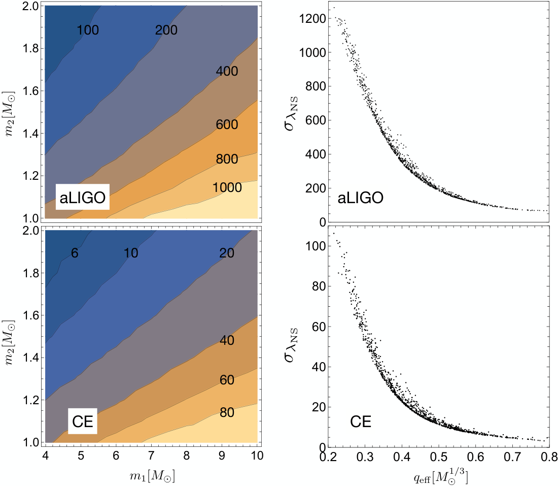
Similarly, Figure 8 shows the measurement errors of the NS tidal deformability for the sources in Pop-I. As in the case of SNR, the error contours also show similar trends between aLIGO and CE. However, the errors seem to depend mainly on the mass ratio rather than the chirp mass. We have verified that the error distribution exhibits the narrowest band if we display the errors as a function of the effective mass ratio defined by , which is shown in the right panel. We performed the same analysis using the TaylorF2 waveform model, and the errors showed a narrower distribution like a thin curve (see Appendix V). We tried to figure out how could be derived from the post-Newtonian equation through the Fisher matrix formalism, but it was unsuccessful. The definition of was empirically chosen from the shape of the contours. Further study is needed for a reasonable explanation, and we leave it for future work. The CE detector can measure the tidal deformability much more accurately than aLIGO, and the error ratios () are distributed in a range .
To see the dependence on the BH spin (), we select three sources with different masses, and for these signals, we calculate the SNRs and the errors varying the true value of in the range . The results are given in Fig. 9. For efficiency, we give the fractional values, where and denote the values of the SNR and the error at , respectively. In the upper panel, the SNR is quite symmetric between positive and negative spins and depends almost linearly on the BH spin for all sources. The variation in is more pronounced for aLIGO and larger for more massive binaries. The largest variation is and at for aLIGO and CE, respectively. In the lower panel, the errors do not show consistent behavior between aLIGO and CE as well as between the sources. The variation in is much larger than the variation in and increases up to in our spin range for both detectors.
Geometrically, an L–Shaped single detector configuration such as LIGO can have two optimal positions and four hidden positions. The optimal positions correspond to the two directions perpendicular to the detector-arms plane, and the hidden positions correspond to the four directions that bisect the detector-arms axes. Figure 10 shows the SNR distribution in the RA–DEC (sky position) plane obtained by using the aLIGO-Hanford (H) and the CE detectors, respectively. Again, we assume the fiducial NSBH source () with a fixed distance () and the optimal orbital orientation (). In the upper panel, the optimal sky positions, where the SNR is maximum, for H and CE are very similar because they are located at a similar site. However, they have different hidden sky positions due to their different orientations. On the other hand, the shape of the PDF curve is almost identical between the two detectors independently of the detector location because the two detectors have the same L-shaped arms and the SNRs are averaged over the entire sky position. The SNR PDF gradually increases in the low region but falls quickly at the end. The SNR value ranges from zero to and is maximum at for aLIGO (CE).
To obtain generalized PDFs of the SNR and , we perform the Fisher matrix analysis on the sources in Pop-I, Pop-II, and Pop-III, respectively. In Fig. 11, we display the PDF of the SNR (top), the PDF of (middle), and its cumulative distribution function (CDF) (bottom). In the top panel, it can be seen that although the parameter space has been extended from two to three dimensions by including the BH spin parameter, there is no noticeable difference between the Pop-I and Pop-II PDFs. This is because the SNR fluctuations due to the BH spin are only a few percent as shown in Fig. 9, and thus the overall distribution is rarely affected by the spin. However, the PDF of Pop-III is more widely distributed in the lower region. In this case, the SNR can have a very small value around the hidden positions. The SNR ranges from to for aLIGO (CE) in both the Pop-I and the Pop-II cases. In the case of Pop-III, the SNR value starts from zero but can increase to the same value as the maximum value of Pop-II when the source is located at the optimal sky position. In the middle panel, the PDF curves of are similar in shape between H and CE but different between the three populations. In the case of Pop-I, the PDF has a sharp peak in the low region and slowly decreases. As the parameter dimension of the population increases, the peak becomes lower and flatter and the tail becomes longer. The errors range broadly from to more than for H (CE), but most errors are concentrated in the low region. The results of for the single-detector analysis are summarized in Table 4. In the case of H, the values of , where the PDF is maximum, are given as and 210, and the values of , where , are given as , and for Pop-I, Pop-II, and Pop-III, respectively, In the case of CE, those are and 15 and , and , respectively. Overall, our results suggest an improvement of about 20 times between H and CE in tidal deformability measurements. On the other hand, Lackey et al.Lackey et al. 2014 also estimated the measurement errors of from NSBH systems for single aLIGO and (L-shaped) ET detectors and found an order of magnitude better accuracy in the case of ET. The PDFs for the other three intrinsic parameters are given in Appendix VI.
| aLIGO (H) | CE | |||||||
|---|---|---|---|---|---|---|---|---|
| Population | ||||||||
| Pop-I | 140 | 220 | 400 | 840 | 9 | 13 | 24 | 55 |
| Pop-II | 190 | 225 | 460 | 1130 | 14 | 12 | 23 | 56 |
| Pop-III | 210 | 360 | 700 | 1500 | 15 | 19 | 39 | 96 |
III.4 Multidetector network analysis
In this subsection, we perform a multi-detector analysis using the networks of the 2G and the 3G detectors, respectively. We adopt the 2G network HLVK consisting of aLIGO-Hanford (H), aLIGO-Livingstone (L), advanced Virgo (V), and KAGRA (K), and the 3G network ETCE consisting of Einstein Telescope (ET) and Cosmic Explorer (CE). In a network, the SNR can be given by
| (15) |
where indicates the SNR of the –th detector. Similarly, the measurement error can be calculated from the network Fisher matrix given by
| (16) |
Figure 12 shows the SNR distribution in the RA–DEC plane obtained by using the 2G and the 3G networks, respectively. We assume the fiducial NSBH source () with a fixed distance () and the optimal orbital orientation. Unlike the single detector case, the trends of the SNR contours are quite different between the 2G and the 3G networks, and there are no hidden positions. The SNR ranges from to for the 2G(3G) network, and the shapes of the PDF curves are significantly different between the two networks. The PDF is maximum at and for the 2G and the 3G networks, respectively.

In Fig. 13, we display the PDF of the SNR (top), the PDF of (middle), and its CDF (bottom) for the sources in Pop-III. In the top panel, the SNR ranges from to for the 2G network and from to for the 3G network. The SNR PDFs are maximum at and for the 2G and the 3G networks, respectively, and they are much larger than those in the single detector case. In the middle and the bottom panels, the overall trends of the PDF and the CDF curves are similar to those in the single detector case, but of the two networks, the 3G network can have a PDF curve with a sharper peak and a longer tail between the two networks. The results of for the multi-detector analysis are summarized in Table 5. The values are given as and and the values are given as and for the 2G and the 3G networks, respectively. The PDFs for the other three intrinsic parameters are given in Appendix VI.
| HLVK | ETCE | |||||||
|---|---|---|---|---|---|---|---|---|
| Population | ||||||||
| Pop-III | 130 | 140 | 260 | 470 | 4 | 10 | 21 | 53 |
III.5 Constraining EOS models
Here, we utilize our results to evaluate how well the theoretical EOS models can be constrained by GW parameter estimation for NSBH signals. We choose four EOS models, WFF1, APR4, SLy, and MPA1 Read et al. 2009, which lie well inside of the credible region of the PDFs for all waveform models used in the analysis of GW170817 Abbott et al. 2019b. In Fig. 14, the upper panel presents the tidal parameter as a function of the NS mass (). For all models, monotonically decreases with increasing NS mass, and the stiffer EOS model gives a higher parameter value for a given NS mass. The parameter values of at are widely distributed from to depending on the EOS model, but they are less than 50 at for all models. The lower panel displays the distribution of for the sources in Pop-III obtained with the 3G network. The error distribution is also wider for smaller NS masses. However, the distribution width is much narrower than that of (in the upper panel) in the low-mass region but is comparable in the high-mass region. This implies that the smaller the NS mass, the better the recovered value of can be constrained between different EOS models.

We provide a concrete example to illustrate how well the EOS models can be distinguished from each other. We prepare a specific population Pop-IV, where Monte Carlo sources are distributed in the 4–D ––RA–DEC space with the NS mass fixed to . For all sources, we assume and . Thus, this population is equivalent to Pop.III except that the NS mass is fixed. For all sources, we obtain the errors from the 6–D Fisher matrices using the 3G network. In Fig. 15, the upper panel shows the CDF curves of for the sources in Pop-IV located at , and , respectively. Note that the results for and can be obtained simply by applying a scale factor as . The horizontal dashed line indicates . We find and 164 for the cases and , respectively, and that means of the sources in Pop-IV satisfy and 164, respectively. These error scales are illustrated in the lower panel, where the gray line indicates the value of according to the EOS model for an NS with , and the error bars correspond to (black), 82 (red), and 164 (blue), respectively. This plot shows the measurability of each EOS model for the sources in Pop-IV located at a certain distance. For example, if enough sources in Pop-IV located at are detected by the 3G network, of their parameter estimation results cannot distinguish the two models SLy and APR4 at the 1– level, where we assume that the true value of is determined by SLy or APR4. On the contrary, if , of the parameter estimation results can distinguish between all EOS models well.
III.6 Dependence on the EOS model
In the above analysis, we adopted the soft EOS model APR4 to choose the true value of . In this subsection, we show how our results can be affected if the true value of is given by other EOS models. To this end, we perform the same Fisher matrix analysis for the sources in Pop-I with the aLIGO PSD using the stiffer EOS model MPA1 Read et al. 2009. The comparison result between APR4 and MPA1 is given in Fig. 16. The upper panel shows the error contours for the soft () and the stiffer () EOS models in the – plane, where the result of is taken from Fig. 8. The result exhibits a highly consistent contour trend between the soft and the stiffer EOS models but shows small differences in the bottom-left region. In the lower panel, the left plot displays the PDFs of for both EOS models. For the same population of sources, the two EOS models provide PDF curves that are similar overall but slightly different. These small differences are well quantified in the right plot, which shows the PDF and the CDF curves of the fractional difference between the error for the stiffer () and the error for the soft () models. We have verified that of the Monte Carlo sources can satisfy , and all of the sources with are concentrated in the bottom-left region (). Therefore, we conclude that the PDF curves obtained in this work are almost unaffected by the choice of the EOS model.
IV Summary and discussion
In this work, we investigated how accurately the NS tidal deformability () can be measured by GW parameter estimation for NSBH signals. For the three populations of NSBH sources distributed in the 2–D – space (Pop–I), the 3–D –– space (Pop–II), and the 5–D –––RA–DEC space (Pop–III), we calculated the measurement errors () using the Fisher matrix method and showed their general distributions as the 1–D PDFs. We chose as our reference waveform model SEOBNR_T, which is one of the recent IMR models including the NS tidal effect, and adopted the four 2G detectors, H, L, V, and K, and the two 3G detectors, ET and CE.
We performed a single-detector analysis for the sources in Pop–I, Pop–II, and Pop–III and compared the SNRs () and the measurement errors () between the aLIGO and the CE detectors. We find that the PDF curves of and are similar in shape between the two detectors, but CE can achieve times better accuracy overall in the measurement of the NS tidal deformability . We also performed a multi-detector analysis using the 2G and the 3G networks for the sources in Pop–III. The PDF curves of are maximum at and for the 2G and the 3G networks, respectively. Overall, the 3G network can achieve times better accuracy in the measurement of . The results for the single and the network detectors are summarized in Tables 4 and 5, respectively. From the results for the Monte Carlo sources distributed in the 4–D ––RA–DEC space with the NS mass fixed to , we found that if , the parameter estimation results for of the sources can distinguish between the EOS models, WFF1, APR4, SLy, and MPA1, at the 1– level, using the 3G network. Finally, we demonstrated that the PDF curves obtained in this work are almost independent of the true value of .
To date, since there are only two NSBH signals, GW200105 and GW200115, detected by the LIGO-Virgo network, it is difficult to predict how many NSBH signals will be detected in the 3G network era. Our PDF curves may not be suitable for direct application to a small number of detection signals because the PDFs represent the statistical distributions obtained by using Monte Carlo samples.
Acknowledgements.
This work was supported by the National Research Foundation of Korea (NRF) grants funded by the Korea government (No. 2018R1D1A1B07048599, No. 2019R1I1A2A01041244, and No. 2020R1C1C1003250)V RESULTS OF THE TaylorF2 WAVEFORM MODEL
Figure 17 shows the SNRs and the measurement errors for the sources in Pop-I obtained by using the TaylorF2 waveform model. We assume to be the frequency at the innermost-stable-circular-orbit. The upper (lower) panel clearly shows the strong dependence of the SNR (error) on the chirp mass (effective mass ratio). These results are obtained by using the same sources (Pop-I) and the same PSD (aLIGO) as in Figs. 7 and 8, hence directly comparable to the results for SEOBNR_T. Note that the results for are significantly different between TaylorF2 and SEOBNR_T, especially in the low mass ratio region, indicating the inadequacy of the TaylorF2 model in our analysis.

VI RESULTS OF THE OTHER INTRINSIC PARAMETERS
In Fig. 18, we present the results of the chirp mass, the symmetric mass ratio, and the BH spin for the sources in Pop-I, Pop-II, and Pop-III, obtained by the single-detector analysis using aLIGO (H) and CE. In Fig. 19, we also present the results of the three parameters for the sources in Pop-III obtained by the multi-detector analysis using the 2G and the 3G networks.
VII ACCURACY OF THE MATRIX INVERSION
We examine the inversion accuracy of our covariance matrix by measuring the matrix norm
| (17) |
where is the identity matrix. If is larger than a certain threshold, the covariance matrix cannot be trusted. We empirically selected the threshold in this work (cf. Gupta et al. 2020). We have verified that almost all NSBH sources used in our 6–D Fisher matrices can satisfy , and we disregarded the sources with values beyond the threshold in our PDFs.
References
- Abbott et al. (2016) B. P. Abbott et al., Observation of gravitational waves from a binary black hole merger, Phys. Rev. Lett. 116, 061102 (2016).
- Aasi et al. (2015) J. Aasi et al., Advanced LIGO, Classical and Quantum Gravity 32, 074001 (2015).
- Acernese et al. (2015) F. Acernese et al., Advanced virgo: a second-generation interferometric gravitational wave detector, Classical and Quantum Gravity 32, 024001 (2015).
- Abbott et al. (2019a) B. P. Abbott et al., Gwtc-1: A gravitational-wave transient catalog of compact binary mergers observed by ligo and virgo during the first and second observing runs, Phys. Rev. X 9, 031040 (2019a).
- Abbott et al. (2021a) R. Abbott et al., Gwtc-2: Compact binary coalescences observed by ligo and virgo during the first half of the third observing run, Phys. Rev. X 11, 021053 (2021a).
- Abbott et al. (2021b) R. Abbott et al., Gwtc-2.1: Deep extended catalog of compact binary coalescences observed by ligo and virgo during the first half of the third observing run, arXiv:2108.01045 (2021b).
- Abbott et al. (2021c) R. Abbott et al., Gwtc-3: Compact binary coalescences observed by ligo and virgo during the second part of the third observing run, arXiv:2111.03606 (2021c).
- Abbott et al. (2017a) B. P. Abbott et al., Gw170817: Observation of gravitational waves from a binary neutron star inspiral, Phys. Rev. Lett. 119, 161101 (2017a).
- Abbott et al. (2019b) B. P. Abbott et al., Properties of the binary neutron star merger gw170817, Phys. Rev. X 9, 011001 (2019b).
- Abbott et al. (2020) B. P. Abbott et al., GW190425: Observation of a compact binary coalescence with total mass 3.4 m, The Astrophysical Journal Letters 892, L3 (2020).
- Abbott et al. (2021d) R. Abbott et al., Observation of gravitational waves from two neutron star–black hole coalescences, The Astrophysical Journal Letters 915, L5 (2021d).
- Foucart (2020) F. Foucart, A brief overview of black hole-neutron star mergers, Frontiers in Astronomy and Space Sciences 7, 10.3389/fspas.2020.00046 (2020).
- Borhanian (2021) S. Borhanian, GWBENCH: a novel fisher information package for gravitational-wave benchmarking, Classical and Quantum Gravity 38, 175014 (2021).
- Lackey et al. (2012) B. D. Lackey, K. Kyutoku, M. Shibata, P. R. Brady, and J. L. Friedman, Extracting equation of state parameters from black hole-neutron star mergers: Nonspinning black holes, Phys. Rev. D 85, 044061 (2012).
- Lackey et al. (2014) B. D. Lackey, K. Kyutoku, M. Shibata, P. R. Brady, and J. L. Friedman, Extracting equation of state parameters from black hole-neutron star mergers: Aligned-spin black holes and a preliminary waveform model, Phys. Rev. D 89, 043009 (2014).
- Kumar et al. (2017) P. Kumar, M. Pürrer, and H. P. Pfeiffer, Measuring neutron star tidal deformability with advanced ligo: A bayesian analysis of neutron star-black hole binary observations, Phys. Rev. D 95, 044039 (2017).
- LIGO Scientific Collaboration (2018) LIGO Scientific Collaboration, LIGO Algorithm Library - LALSuite, free software (GPL) (2018).
- Pürrer (2014) M. Pürrer, Frequency-domain reduced order models for gravitational waves from aligned-spin compact binaries, Classical and Quantum Gravity 31, 195010 (2014).
- Bohé et al. (2017) A. Bohé et al., Improved effective-one-body model of spinning, nonprecessing binary black holes for the era of gravitational-wave astrophysics with advanced detectors, Phys. Rev. D 95, 044028 (2017).
- Smith et al. (2016) R. Smith, S. E. Field, K. Blackburn, C.-J. Haster, M. Pürrer, V. Raymond, and P. Schmidt, Fast and accurate inference on gravitational waves from precessing compact binaries, Phys. Rev. D 94, 044031 (2016).
- Dietrich et al. (2017) T. Dietrich, S. Bernuzzi, and W. Tichy, Closed-form tidal approximants for binary neutron star gravitational waveforms constructed from high-resolution numerical relativity simulations, Phys. Rev. D 96, 121501 (2017).
- Dietrich et al. (2019) T. Dietrich, A. Samajdar, S. Khan, N. K. Johnson-McDaniel, R. Dudi, and W. Tichy, Improving the nrtidal model for binary neutron star systems, Phys. Rev. D 100, 044003 (2019).
- Matas et al. (2020) A. Matas, T. Dietrich, A. Buonanno, T. Hinderer, M. Pürrer, F. Foucart, M. Boyle, M. D. Duez, L. E. Kidder, H. P. Pfeiffer, and M. A. Scheel, Aligned-spin neutron-star–black-hole waveform model based on the effective-one-body approach and numerical-relativity simulations, Phys. Rev. D 102, 043023 (2020).
- Pannarale et al. (2015) F. Pannarale, E. Berti, K. Kyutoku, B. D. Lackey, and M. Shibata, Aligned spin neutron star-black hole mergers: A gravitational waveform amplitude model, Phys. Rev. D 92, 084050 (2015).
- Hannam et al. (2014) M. Hannam, P. Schmidt, A. Bohé, L. Haegel, S. Husa, F. Ohme, G. Pratten, and M. Pürrer, Simple model of complete precessing black-hole-binary gravitational waveforms, Phys. Rev. Lett. 113, 151101 (2014).
- Husa et al. (2016) S. Husa, S. Khan, M. Hannam, M. Pürrer, F. Ohme, X. J. Forteza, and A. Bohé, Frequency-domain gravitational waves from nonprecessing black-hole binaries. i. new numerical waveforms and anatomy of the signal, Phys. Rev. D 93, 044006 (2016).
- Khan et al. (2016) S. Khan, S. Husa, M. Hannam, F. Ohme, M. Pürrer, X. J. Forteza, and A. Bohé, Frequency-domain gravitational waves from nonprecessing black-hole binaries. ii. a phenomenological model for the advanced detector era, Phys. Rev. D 93, 044007 (2016).
- Thompson et al. (2020) J. E. Thompson, E. Fauchon-Jones, S. Khan, E. Nitoglia, F. Pannarale, T. Dietrich, and M. Hannam, Modeling the gravitational wave signature of neutron star black hole coalescences, Phys. Rev. D 101, 124059 (2020).
- Santamaría et al. (2010) L. Santamaría, F. Ohme, P. Ajith, B. Brügmann, N. Dorband, M. Hannam, S. Husa, P. Mösta, D. Pollney, C. Reisswig, E. L. Robinson, J. Seiler, and B. Krishnan, Matching post-newtonian and numerical relativity waveforms: Systematic errors and a new phenomenological model for nonprecessing black hole binaries, Phys. Rev. D 82, 064016 (2010).
- Veitch et al. (2015) J. Veitch, V. Raymond, B. Farr, W. Farr, P. Graff, S. Vitale, et al., Parameter estimation for compact binaries with ground-based gravitational-wave observations using the lalinference software library, Phys. Rev. D 91, 042003 (2015).
- Finn (1992) L. S. Finn, Detection, measurement, and gravitational radiation, Phys. Rev. D 46, 5236 (1992).
- Cutler and Flanagan (1994) C. Cutler and E. E. Flanagan, Gravitational waves from merging compact binaries: How accurately can one extract the binary’s parameters from the inspiral waveform?, Phys. Rev. D 49, 2658 (1994).
- Allen et al. (2012) B. Allen, W. G. Anderson, P. R. Brady, D. A. Brown, and J. D. E. Creighton, Findchirp: An algorithm for detection of gravitational waves from inspiraling compact binaries, Phys. Rev. D 85, 122006 (2012).
- Cho et al. (2013) H.-S. Cho, E. Ochsner, R. O’Shaughnessy, C. Kim, and C.-H. Lee, Gravitational waves from black hole-neutron star binaries: Effective fisher matrices and parameter estimation using higher harmonics, Phys. Rev. D 87, 024004 (2013).
- Baird et al. (2013) E. Baird, S. Fairhurst, M. Hannam, and P. Murphy, Degeneracy between mass and spin in black-hole-binary waveforms, Phys. Rev. D 87, 024035 (2013).
- Cho and Lee (2014) H.-S. Cho and C.-H. Lee, Application of the effective fisher matrix to the frequency domain inspiral waveforms, Classical and Quantum Gravity 31, 235009 (2014).
- Cho (2015) H.-S. Cho, Parameter estimation using a complete signal and inspiral templates for low-mass binary black holes with advanced LIGO sensitivity, Classical and Quantum Gravity 32, 235007 (2015).
- Jaranowski and Krolak (1994) P. Jaranowski and A. Krolak, Optimal solution to the inverse problem for the gravitational wave signal of a coalescing compact binary, Phys. Rev. D 49, 1723 (1994).
- Vallisneri (2008) M. Vallisneri, Use and abuse of the fisher information matrix in the assessment of gravitational-wave parameter-estimation prospects, Phys. Rev. D 77, 042001 (2008).
- Porter (2002) E. K. Porter, Computational resources to filter gravitational wave data with p-approximant templates, Classical and Quantum Gravity 19, 4343 (2002).
- Poisson and Will (1995) E. Poisson and C. M. Will, Gravitational waves from inspiraling compact binaries: Parameter estimation using second-post-newtonian waveforms, Phys. Rev. D 52, 848 (1995).
- Rodriguez et al. (2013) C. L. Rodriguez, B. Farr, W. M. Farr, and I. Mandel, Inadequacies of the fisher information matrix in gravitational-wave parameter estimation, Phys. Rev. D 88, 084013 (2013).
- Mandel et al. (2014) I. Mandel, C. P. L. Berry, F. Ohme, S. Fairhurst, and W. M. Farr, Parameter estimation on compact binary coalescences with abruptly terminating gravitational waveforms, Classical and Quantum Gravity 31, 155005 (2014).
- Harry and Lundgren (2021) I. Harry and A. Lundgren, Failure of the fisher matrix when including tidal terms: Considering construction of template banks of tidally deformed binary neutron stars, Phys. Rev. D 104, 043008 (2021).
- Cho (2022a) H.-S. Cho, Improvement of the parameter measurement accuracy by the third-generation gravitational wave detector einstein telescope, Classical and Quantum Gravity 39, 085006 (2022a).
- Burgay et al. (2003) M. Burgay et al., An increased estimate of the merger rate of double neutron stars from observations of a highly relativistic system, Nature 426, 531 (2003).
- Stovall et al. (2018) K. Stovall et al., PALFA discovery of a highly relativistic double neutron star binary, The Astrophysical Journal 854, L22 (2018).
- Read et al. (2009) J. S. Read, B. D. Lackey, B. J. Owen, and J. L. Friedman, Constraints on a phenomenologically parametrized neutron-star equation of state, Phys. Rev. D 79, 124032 (2009).
- Aso et al. (2013) Y. Aso, Y. Michimura, K. Somiya, M. Ando, O. Miyakawa, T. Sekiguchi, D. Tatsumi, and H. Yamamoto (The KAGRA Collaboration), Interferometer design of the kagra gravitational wave detector, Phys. Rev. D 88, 043007 (2013).
- Abbott et al. (2017b) B. P. Abbott et al., Exploring the sensitivity of next generation gravitational wave detectors, Classical and Quantum Gravity 34, 044001 (2017b).
- Punturo et al. (2010) M. Punturo et al., The einstein telescope: a third-generation gravitational wave observatory, Classical and Quantum Gravity 27, 194002 (2010).
- Ashton et al. (2019) G. Ashton et al., Bilby: A user-friendly bayesian inference library for gravitational-wave astronomy, The Astrophysical Journal Supplement Series 241, 27 (2019).
- Speagle (2020) J. S. Speagle, dynesty: a dynamic nested sampling package for estimating bayesian posteriors and evidences, Monthly Notices of the Royal Astronomical Society 493, 3132 (2020).
- Morisaki (2021) S. Morisaki, Accelerating parameter estimation of gravitational waves from compact binary coalescence using adaptive frequency resolutions, Phys. Rev. D 104, 044062 (2021).
- Cho (2022b) H.-S. Cho, Systematic bias due to eccentricity in parameter estimation for merging binary neutron stars, Phys. Rev. D 105, 124022 (2022b).
- Gupta et al. (2020) A. Gupta, S. Datta, S. Kastha, S. Borhanian, K. G. Arun, and B. S. Sathyaprakash, Multiparameter tests of general relativity using multiband gravitational-wave observations, Phys. Rev. Lett. 125, 201101 (2020).