跳到论文正文
W Papers独立论文阅读器 arXiv:2210.02560 论文正文 计算阅读时间 · 0%
引用这篇论文根据当前论文元数据生成,正式投稿前建议核对。


License: CC BY 4.0
arXiv:2210.02560v1 [math.DS] 05 Oct 2022

Bifurcation analysis of Bogdanov-Takens bifurcations in delay differential equationsThanks: Submitted to the editors DATE.

M.M. Bosschaert Thanks: Department of Mathematics, Hasselt University, Diepenbeek Campus, Agoralaan Gebouw D, 3590 Diepenbeek, Belgium (\emailmaikel.bosschaert@uhasselt.be).    Yu.A. Kuznetsov Thanks: Department of Mathematics, Utrecht University, Budapestlaan 6, 3508 TA Utrecht, The Netherlands and Department of Applied Mathematics, University of Twente, Zilverling Building, 7500AE Enschede, The Netherlands (\emailI.A.Kouznetsov@uu.nl).
Abstract

In this paper, we will perform the parameter-dependent center manifold reduction near the generic and transcritical codimension two Bogdanov–Takens bifurcation in classical delay differential equations (DDEs). Using a generalization of the Lindstedt-Poincaré method to approximate the homoclinic solution allows us to initialize the continuation of the homoclinic bifurcation curves emanating from these points. The normal form transformation is derived in the functional analytic perturbation framework for dual semigroups (sun-star calculus) using a normalization technique based on the Fredholm alternative. The obtained expressions give explicit formulas, which have been implemented in the freely available bifurcation software package DDE-BifTool. The effectiveness is demonstrated on various models.

{keywords}

generic Bogdanov–Takens bifurcation, transcritical Bogdanov–Takens bifurcation, homoclinic solutions, delay differential equations, sun-star calculus, strongly continuous semi-groups, Center Manifold Theorem, DDE-BifTool

{AMS}

37G05, 37G10, 65P30, 34K16, 34K18, 34K19

1 Introduction

The Bogdanov–Takens bifurcation caused by the presence of an equilibrium with a double zero eigenvalue is a well-studied singularity in dynamical systems. It implies existence of saddle homoclinic orbits nearby, which is a global phenomenon. In particular, the codimension two Bogdanov–Takens bifurcation in finite-dimensional ordinary differential equations (ODEs) has been studied theoretically and applied in numerous reserach publications. The same is true for the infinite-dimensional dynamical systems generated by delay differential equations (DDEs). In the simplest case, often encountered in applications, such DDEs have the form

x˙​(t)=f⁡(x⁡(t),x⁡(t−τ1),…,x⁡(t−τm),α),t≥0,\dot{x}(t)=f(x(t),x(t-\tau_{1}),\ldots,x(t-\tau_{m}),\alpha),\qquad t\geq 0, (1)

where x⁡(t)∈ℝn,α∈ℝpx(t)\in\mathbb{R}^{n},\ \alpha\in\mathbb{R}^{p}, while 0<τ1<τ2<⋯<τm0<\tau_{1}<\tau_{2}<\cdots<\tau_{m} are constant delays, and f:ℝn×(m+1)×ℝp→ℝnf:\mathbb{R}^{n\times(m+1)}\times\mathbb{R}^{p}\to\mathbb{R}^{n} is a smooth mapping. These are known as discrete DDEs.

Up to date, the standard available parameter-dependent center manifold theorem for DDEs in [13] assumed that the equilibrium persists for all nearby parameter values. This was a serious limitation, since in generic unfoldings of the codimension two Bogdanov–Takens singularity it is not the case.

However, recently, in [2], this obstruction has been removed and the existence of finite-dimensional smooth parameter-dependent local center manifolds has been rigorously established in the functional analytic perturbation framework for dual semigroups (sun-star calculus) developed in [5, 6, 7, 8]. Once the existence of these invariant manifolds is proved, the normalization technique for local bifurcations of ODEs developed in [27] can be lifted rather easily to the infinite dimensional setting of DDEs. The advantages of this normalization technique are that the center manifold reduction and the calculation of the normal form coefficients are performed simultaneously by solving the so-called homological equation. This method gives explicit expressions for the coefficients rather than a procedure as developed in [17, 18]. The explicit expressions make them particularly suitable for both symbolic and numerical evaluation.

Indeed, utilizing the normalization method, the authors in [2] obtained asymptotics to initialize the continuation of codimension one bifurcation curves of nonhyperbolic equilibria and cycles emanating from the codimension two generalized Hopf, fold-Hopf, Hopf-Hopf and transcritical-Hopf bifurcation points in DDEs of the form Eq. 1. These asymptotics have been implemented into the fully GNU Octave compatible MATLAB package DDE-BifTool [16, 35].

Another recent developent is the rigorous derivation of higher-order asymptotics for the codimension one homoclinic bifurcation curve emanating from the generic codimension two Bogdanov–Takens bifurcation point in in two-parameter ODEs [3]. Thus, by combining the results of the parameter-dependent center manifolds in DDEs from [2] and the homoclinic asymptotics in ODEs from [3], we are in the position to perform the parameter-dependent center manifold reduction and normalization for the generic and transcritical codimension two Bogdanov–Takens bifurcations. This will allow us to initialize the continuation of codimension one bifurcation curves of nonhyperbolic equilibria and homoclinic solutions emanating from these codimension two points. Hopefully, our results and their software implementation will make the numerical analysis of Bogdanov–Takens bifurcations in DDEs from applications rather routine.

This paper is organized as follows. We begin in Section 2 with a short summary from [2] on parameter-dependent center manifolds for classical DDEs and we state various results needed for the normalization technique. In Section 3 we describe the general technique that we use to derive the transformation from the orbital normal form on the parameter-dependent center manifold in the infinite-dimensional setting of DDEs. In Section 4 the method is then applied to the generic and transcritical codimension two Bogdanov–Takens bifurcations. We provide explicit transformations necessary for the predictors of codimension one bifurcation curves. We do this in a form suitable for classical DDEs, covering cases that are more general than Eq. 1. It is here where we see the true benefit of allowing for orbital normal forms on the center manifold. Indeed, we do not need to derive homoclinic asymptotics for the transcritical codimension two Bogdanov–Takens bifurcation separately. Instead, we only need to derive the center manifold transformation for the transcritical codimension two Bogdanov–Takens bifurcation. Then, using the blow-up transformations Eq. 82, we obtain the same perturbed Hamiltonian system (up to order three) as in the generic Bogdanov–Takens bifurcation.

We employ our implementation in DDE-BifTool to illustrate the accuracy of the codimension one bifurcation curve predictors through various example models, displaying the generic and transcritical codimension two Bogdanov–Takens bifurcations in Section 5. An in-depth treatment of the examples, including the MATLAB and Julia source code to reproduce the obtained results, as well as a more in-depth analysis of the examples, are provided in the Supplement.

2 Parameter-dependent center manifolds for DDEs

Here we summarize those results from [2] on parameter-dependent center manifold for classical DDEs, which are required for the normalization technique in Section 4. For a general introduction on perturbation theory for dual semigroups (also known as sun-star calculus) we refer to [13].

Consider the classical parameter-dependent DDE

x˙​(t)=F⁡(xt,α),t≥0,\dot{x}(t)=F(x_{t},\alpha),\qquad t\geq 0, (DDE)

where F:X×ℝp→ℝnF:X\times\mathbb{R}^{p}\to\mathbb{R}^{n} is CkC^{k}-smooth for some k≥1k\geq 1 with F⁡(0,0)=0F(0,0)=0 and X≔C⁡([−h,0],ℝn)X\coloneqq C([-h,0],\mathbb{R}^{n}). Here for each t≥0t\geq 0, the history function xt:[−h,0]→ℝnx_{t}:[-h,0]\to\mathbb{R}^{n} defined by

xt​(θ)≔x⁡(t+θ),∀θ∈[−h,0].x_{t}(\theta)\coloneqq x(t+\theta),\qquad\forall\,\theta\in[-h,0].

It is convenient to split the right hand-side into its linear and nonlinear parts and write

F⁡(ϕ,α)=⟨ζ,ϕ⟩+D2​F​(0,0)​α+G⁡(xt,α).F(\phi,\alpha)=\langle\zeta,\phi\rangle+D_{2}F(0,0)\alpha+G(x_{t},\alpha). (2)

Here ζ:[0,h]→ℝn×n\zeta:[0,h]\to\mathbb{R}^{n\times n} is a matrix-valued function of bounded variation, normalized by the requirement that ζ⁡(0)=0\zeta(0)=0 and is right-continuous on the open interval (0,h)(0,h), and G:X→ℝnG:X\to\mathbb{R}^{n} is a CkC^{k}-smooth nonlinear operator with G⁡(0,0)=G1​(0,0)=G2​(0,0)=0G(0,0)=G_{1}(0,0)=G_{2}(0,0)=0. The pairing is defined by

⟨ζ,ϕ⟩≔∫0hd​ζ​(θ)​ϕ​(−θ),\langle\zeta,\phi\rangle\coloneqq\int_{0}^{h}{d\zeta(\theta)\phi(-\theta}), (3)

where the integral is of the Riemann–Stieltjes type.

Let TT be the 𝒞0\mathcal{C}_{0}-semigroup on XX corresponding to the linearization of Eq. DDE at 0∈X0\in X for the critical parameter value α=0\alpha=0. Suppose that the generator

𝒟(A)={ϕ∣ϕ˙∈X,ϕ˙(0)=⟨ζ,ϕ⟩},Aϕ=ϕ˙,\mathcal{D}{(A)}=\{\phi\mid\dot{\phi}\in X,\dot{\phi}(0)=\langle\zeta,\phi\rangle\},\qquad A\phi=\dot{\phi},

of TT has 1≤n0<∞1\leq n_{0}<\infty purely imaginary eigenvalues with corresponding n0n_{0}-dimensional real center eigenspace X0X_{0}. Then by [2, Corollary 20] there exists a CkC^{k}-smooth map 𝒞:U×Up→X\mathcal{C}:U\times U_{p}\to X defined in a neighborhood of the origin in X0×ℝpX_{0}\times\mathbb{R}^{p} and such that for every sufficiently small α∈ℝp\alpha\in\mathbb{R}^{p} the manifold 𝒲locc​(α)≔𝒞⁡(U,α)\mathcal{W}^{c}_{\text{loc}}(\alpha)\coloneqq\mathcal{C}(U,\alpha) is locally positively invariant for the semiflow generated by Eq. DDE at parameter value α\alpha.

Since XX is not reflexive, i.e. does not isomorphic to its dual space X⋆X^{\star}, the adjoint semigroup T⋆T^{\star} is only weak⋆\text{weak}^{\star} continuous on X⋆X^{\star} and A⋆A^{\star} generates T⋆T^{\star} only in the weak⋆\text{weak}^{\star} sense. The maximal subspace of strong continuity

X⊙≔{x⋆∈X⋆:t↦T⋆​(t)​x⋆​ is norm-continuous on ​ℝ+}X^{\odot}\coloneqq\left\{x^{\star}\in X^{\star}\,:\,t\mapsto T^{\star}(t)x^{\star}\text{ is norm-continuous on }\mathbb{R}_{+}\right\}

is invariant under T⋆T^{\star}, and we have the representation

X⊙=ℝn⋆×L1([0,h],ℝn⋆).X^{\odot}=\mathbb{R}^{n\star}\times L^{1}([0,h],\mathbb{R}^{n\star}). (4)

The duality pairing between ϕ⊙=(c,g)∈X⊙\phi^{\odot}=(c,g)\in X^{\odot} and ϕ∈X\phi\in X is

⟨ϕ⊙,ϕ⟩=c​ϕ​(0)+∫0hg⁡(θ)​ϕ​(−θ)​𝑑θ.\langle\phi^{\odot},\phi\rangle=c\phi(0)+\int_{0}^{h}g(\theta)\,\phi(-\theta)\,d\theta. (5)

At this stage, we again have a 𝒞0\mathcal{C}_{0}-semigroup T⊙T^{\odot} with generator A⊙A^{\odot} on a Banach space X⊙X^{\odot} so we can iterate the above construction once more. On the dual space

X⊙⁣⋆=ℝn×L∞​([−h,0],ℝn),X^{\odot\star}=\mathbb{R}^{n}\times L^{\infty}([-h,0],\mathbb{R}^{n}),

we obtain the adjoint semigroup T⊙⁣⋆T^{\odot\star} with the weak⋆\text{weak}^{\star} generator

𝒟⁡(A⊙⁣⋆)={(α,ϕ)∈X⊙⁣⋆∣ϕ∈Lip⁡(α)},A⊙⁣⋆​(α,ϕ)=(⟨ζ,ϕ⟩,ϕ˙).\mathcal{D}{(A^{\odot\star})}=\{(\alpha,\phi)\in X^{\odot\star}\mid\phi\in\LIP(\alpha)\},\qquad A^{\odot\star}(\alpha,\phi)=(\langle\zeta,\phi\rangle,\dot{\phi}). (6)

The duality pairing between ϕ⊙⁣⋆=(a,ψ)∈X⊙⁣⋆\phi^{\odot\star}=(a,\psi)\in X^{\odot\star} and ϕ⊙=(c,g)∈X⊙\phi^{\odot}=(c,g)\in X^{\odot} is

⟨ϕ⊙⁣⋆,ϕ⊙⟩=c​a+∫0hg⁡(θ)​ψ​(−θ)​𝑑θ.\langle\phi^{\odot\star},\phi^{\odot}\rangle=ca+\int_{0}^{h}g(\theta)\,\psi(-\theta)\,d\theta. (7)

By restriction to the maximal subspace of strong continuity X⊙⁣⊙=𝒟⁡(A⊙⁣⋆)¯X^{\odot\odot}=\overline{\mathcal{D}(A^{\odot\star})}, we end up with the 𝒞\mathcal{C}-semigroup T⊙⁣⊙T^{\odot\odot}. Its generator A⊙⁣⊙A^{\odot\odot} is the part of A⊙⁣⋆A^{\odot\star} in X⊙⁣⊙X^{\odot\odot}. The canonical injection j:X→X⊙⁣⋆j:X\to X^{\odot\star} is given by

j⁡(ϕ)=(ϕ⁡(0),ϕ),j(\phi)=\left(\phi(0),\phi\right), (8)

mapping XX onto X⊙⁣⊙X^{\odot\odot}. Therefore, XX is sun-reflexive with respect to the shift semigroup TT.

We are now in the position to state the second part of [2, Corollary 20]. That is, if the history xtx_{t} associated with a solution of Eq. DDE exists on some nondegenerate interval II and xt∈𝒲locc​(α)x_{t}\in\mathcal{W}^{c}_{\text{loc}}(\alpha) for all t∈It\in I, then u:I→Xu:I\to X defined by u⁡(t)≔xtu(t)\coloneqq x_{t} is differentiable and satisfies

j​u˙​(t)=A⊙⁣⋆​j​u​(t)+(D2​F​(0,0)​α)​r⊙⁣⋆+G⁡(u⁡(t),α)​r⊙⁣⋆,∀t∈I.j\dot{u}(t)=A^{\odot\star}ju(t)+(D_{2}F(0,0)\alpha)r^{\odot\star}+G(u(t),\alpha)r^{\odot\star},\qquad\forall\,t\in I.

Here, for i=1,…,ni=1,\ldots,n, we denote ri⊙⁣⋆≔(ei,0)r^{\odot\star}_{i}\coloneqq(e_{i},0), where eie_{i} is the iith standard basis vector of ℝn\mathbb{R}^{n} and

w​r⊙⁣⋆≔∑i=1nwi​ri⊙⁣⋆,∀w=(w1,…,wn)∈ℝn.wr^{\odot\star}\coloneqq\sum_{i=1}^{n}{w_{i}r^{\odot\star}_{i}},\qquad\forall\,w=(w_{1},\ldots,w_{n})\in\mathbb{R}^{n}.

2.1 Spectral computations for classical DDEs in case of multiple eigenvalues

It is well known that for classical DDEs all spectral information about the generator AA is contained in a holomorphic characteristic matrix function Δ:ℂ→ℂn×n\Delta:\mathbb{C}\to\mathbb{C}^{n\times n} defined by

Δ⁡(z)≔z​I−ζ^​(z)withζ^​(z)≔∫0he−z​θ​𝑑ζ​(θ),\Delta(z)\coloneqq zI-\hat{\zeta}(z)\qquad\text{with}\qquad\hat{\zeta}(z)\coloneqq\int_{0}^{h}{e^{-z\theta}\,d\zeta(\theta)}, (9)

where ζ\zeta is the real kernel from Eq. 3, see [13, Sections IV.4 and IV.5]. In particular, the eigenvalues of AA are the roots of the characteristic equation

det⁡Δ⁡(z)=0,\operatorname{det}{\Delta(z)}=0, (10)

and the algebraic multiplicity of an eigenvalue equals its order as a root of Eq. 10.

For the normalization technique in Section 4, we will need normalized representations for the (generalized) eigenfunctions and adjoint (generalized) eigenfunctions of the generator AA and A⋆A^{\star}, respectively. In this section, we will consider the more general case where λ\lambda is an eigenvalue of algebraic multiplicity k∈ℕk\in\mathbb{N} and geometric multiplicity 1. Although in Section 4 we will only need the special case where λ=0\lambda=0 is a double eigenvalue of AA, the expressions are useful when considering for example the 1:1 resonant Hopf bifurcation and the triple zero bifurcation.

{proposition}

Let λ\lambda be an eigenvalue of the generator AA with algebraic multiplicity k∈ℕk\in\mathbb{N} and geometric multiplicity one, then there are ((generalized )) eigenfunctions ϕi\phi_{i} such that

A​ϕ0=λ​ϕ0,A​ϕi=λ​ϕi+ϕi−1,i∈{1,…,k−1},A\phi_{0}=\lambda\phi_{0},\qquad A\phi_{i}=\lambda\phi_{i}+\phi_{i-1},\qquad i\in\{1,\dots,k-1\}, (11)

and adjoint ((generalized )) eigenfunctions ψi\psi_{i} such that

A⋆​ψk−1=λ​ψk−1,A⋆​ψk−i=λ​ψk−i+ψk−i+1,i∈{2,…,k}.A^{\star}\psi_{k-1}=\lambda\psi_{k-1},\qquad A^{\star}\psi_{k-i}=\lambda\psi_{k-i}+\psi_{k-i+1},\qquad i\in\{2,\dots,k\}. (12)

Let the ordered set (q0,…,qk−1)(q_{0},\dots,q_{k-1}) of vectors be a Jordan chain for Δ⁡(λ)\Delta(\lambda), i.e. q0≠0q_{0}\neq 0 and

Δ⁡(z)​[q0+(z−λ)​q1+⋯+(z−λ)k​qk−1]=𝒪⁡((z−λ)k).\Delta(z)[q_{0}+(z-\lambda)q_{1}+\cdots+(z-\lambda)^{k}q_{k-1}]=\mathcal{O}((z-\lambda)^{k}).

Similarly, let (pk−1,…,p0)(p_{k-1},\dots,p_{0}) be a Jordan chain for ΔT​(λ)\Delta^{T}(\lambda). Then the ((generalized ))) eigenfunctions and adjoint ((generalized )) eigenfunctions are given by

ϕi:[−h,0]→ℝn\displaystyle\phi_{i}\colon[-h,0]\rightarrow\mathbb{R}^{n} :θ↦eλ​θ​∑l=0iqi−l​θll!,\displaystyle\colon\theta\mapsto e^{\lambda\theta}\sum_{l=0}^{i}q_{i-l}\frac{\theta^{l}}{l!}, (13)
ψi:[0,h]→ℝn\displaystyle\psi_{i}\colon[0,h]\rightarrow\mathbb{R}^{n} :θ↦pi+∑l=0k−1−ipi+l​∫0θ∫σheλ⁡(σ−s)​(σ−s)ll!​dζ​(s)​dσ,\displaystyle\colon\theta\mapsto p_{i}+\sum_{l=0}^{k-1-i}p_{i+l}\int_{0}^{\theta}\int_{\sigma}^{h}e^{\lambda(\sigma-s)}\frac{(\sigma-s)^{l}}{l!}d\zeta(s)d\sigma,

for i∈{0,…,k−1}i\in\{0,\dots,k-1\}, respectively. Furthermore, the following identities hold

⟨ψi,ϕj⟩\displaystyle\left<\psi_{i},\phi_{j}\right> =⟨ψi+1,ϕj+1⟩,\displaystyle=\left<\psi_{i+1},\phi_{j+1}\right>, i,j∈{0,…,k−2},\displaystyle i,j\in\{0,\dots,k-2\}, (14)
⟨ψk−1,ϕk−1⟩\displaystyle\left<\psi_{k-1},\phi_{k-1}\right> =pk−1​∑l=0k−1Δ(l+1)​(λ)(l+1)!​qk−1−l,\displaystyle=p_{k-1}\sum_{l=0}^{k-1}\frac{\Delta^{(l+1)}(\lambda)}{(l+1)!}q_{k-1-l},
⟨ψi,ϕj⟩\displaystyle\left<\psi_{i},\phi_{j}\right> =0,\displaystyle=0, i>j,\displaystyle i>j,
⟨ψ0,ϕj⟩\displaystyle\left<\psi_{0},\phi_{j}\right> =∑l=0k−1∑m=0jpl​Δ(l+m+1)​(λ)(l+m+1)!​qj−m,\displaystyle=\sum_{l=0}^{k-1}\sum_{m=0}^{j}p_{l}\frac{\Delta^{(l+m+1)}(\lambda)}{(l+m+1)!}q_{j-m}, j>0,\displaystyle j>0,

which can be normalized to satisfy

⟨ψi,ϕj⟩=δi​j.\langle\psi_{i},\phi_{j}\rangle=\delta_{ij}. (15)
Proof.

The (generalized) eigenspace at an eigenvalue λ\lambda of AA of algebraic multiplicity kk and geometric multiplicity 1 is given by

𝒩⁡((A−λ)k),\mathcal{N}((A-\lambda)^{k}),

which leads to the expressions in Eq. 11 and similarly for Eq. 12. The representations of the (generalized) eigenfunctions and adjoint (generalized) eigenfunctions can be found in Theorem IV.5.5 and IV.5.9 in [13], respectively.

The first identity in Eq. 14 follows directly from

⟨ψi+1,ϕj+1⟩=⟨(λ−A⋆)​ψi,ϕj+1⟩=⟨ψi,(λ−A)​ϕj+1⟩=⟨ψi,ϕj⟩,\left<\psi_{i+1},\phi_{j+1}\right>=\left<(\lambda-A^{\star})\psi_{i},\phi_{j+1}\right>=\left<\psi_{i},(\lambda-A)\phi_{j+1}\right>=\left<\psi_{i},\phi_{j}\right>,

where i,j∈{0,…,k−2}i,j\in\{0,\dots,k-2\}. For the second identity in Eq. 14 we notice that

⟨ψk−1,ϕk−1⟩\displaystyle\left<\psi_{k-1},\phi_{k-1}\right> =∫0hd​ψk−1​(θ)​ϕk−1​(−θ)=pk−1​q0+∫0hψk−1′​(θ)​ϕk−1​(−θ)​𝑑θ\displaystyle=\int_{0}^{h}d\psi_{k-1}(\theta)\phi_{k-1}(-\theta)=p_{k-1}q_{0}+\int_{0}^{h}\psi^{\prime}_{k-1}(\theta)\phi_{k-1}(-\theta)d\theta
=pk−1​q0+∫0hpk−i​∫θheλ⁡(θ−s)​𝑑ζ​(s)​e−λ​θ​∑l=0k−1qi−l​(−1)l​θll!​𝑑θ\displaystyle=p_{k-1}q_{0}+\int_{0}^{h}p_{k-i}\int_{\theta}^{h}e^{\lambda(\theta-s)}d\zeta(s)e^{-\lambda\theta}\sum_{l=0}^{k-1}q_{i-l}\frac{(-1)^{l}\theta^{l}}{l!}d\theta
=pk−1​q0+pk−i​∑l=0k−1∫0h∫θhe−λ​s​(−1)l​θll!​𝑑ζ​(s)​𝑑θ​qi−l\displaystyle=p_{k-1}q_{0}+p_{k-i}\sum_{l=0}^{k-1}\int_{0}^{h}\int_{\theta}^{h}e^{-\lambda s}\frac{(-1)^{l}\theta^{l}}{l!}d\zeta(s)d\theta q_{i-l}
=pk−1​q0+pk−i​∑l=0k−1∫0h∫0se−λ​s​(−1)l​θll!​𝑑θ​𝑑ζ​(s)​qi−l\displaystyle=p_{k-1}q_{0}+p_{k-i}\sum_{l=0}^{k-1}\int_{0}^{h}\int_{0}^{s}e^{-\lambda s}\frac{(-1)^{l}\theta^{l}}{l!}d\theta d\zeta(s)q_{i-l}
=pk−1​q0+pk−i​∑l=0k−1∫0he−λ​s​(−1)l​sl+1(l+1)!​𝑑ζ​(s)​qi−l=pk−1​∑l=0k−1OPENΔ(lCLOSE)​(λ)(l+1)!​qi−l,\displaystyle=p_{k-1}q_{0}+p_{k-i}\sum_{l=0}^{k-1}\int_{0}^{h}e^{-\lambda s}\frac{(-1)^{l}s^{l+1}}{(l+1)!}d\zeta(s)q_{i-l}=p_{k-1}\sum_{l=0}^{k-1}\frac{\Delta^{(l})(\lambda)}{(l+1)!}q_{i-l},

where we used Fubini’s theorem to change the order of integration. The last equality holds since

Δ′​(z)=z​I+∫0hθ​e−z​θ​𝑑ζ​(θ)\Delta^{\prime}(z)=zI+\int_{0}^{h}{\theta e^{-z\theta}\,d\zeta(\theta)}

and

Δ(n)​(z)=(−1)n+1​∫0hθn​e−z​θ​𝑑ζ​(θ),n>1.\Delta^{(n)}(z)=(-1)^{n+1}\int_{0}^{h}{\theta^{n}e^{-z\theta}\,d\zeta(\theta)},\quad n>1.

Using the first identity in Eq. 14 and that for j>0j>0 we have

⟨ψj,ϕ0⟩=⟨(λ−A⋆)​ψj−1,ϕ0⟩=⟨ψj−1,(λ−A)​ϕ0⟩=0,\displaystyle\left<\psi_{j},\phi_{0}\right>=\left<(\lambda-A^{\star})\psi_{j-1},\phi_{0}\right>=\left<\psi_{j-1},(\lambda-A)\phi_{0}\right>=0,

the third identity in Eq. 14 follows.

For the last identity in Eq. 14, we have that

⟨ψ0,ϕj⟩\displaystyle\left<\psi_{0},\phi_{j}\right> =∫0hd​ψ0​(θ)​ϕj​(−θ)=p0​qj+∫0hψ0′​(θ)​ϕj​(−θ)​𝑑θ\displaystyle=\int_{0}^{h}d\psi_{0}(\theta)\phi_{j}(-\theta)=p_{0}q_{j}+\int_{0}^{h}\psi^{\prime}_{0}(\theta)\phi_{j}(-\theta)d\theta
=p0​qj+∫0h(∑l=0k−1pl​∫θheλ⁡(θ−s)​(θ−s)ll!​𝑑ζ​(s)​e−λ​θ​∑m=0jqj−m​(−1)m​θmm!)​𝑑θ\displaystyle=p_{0}q_{j}+\int_{0}^{h}\left(\sum_{l=0}^{k-1}p_{l}\int_{\theta}^{h}e^{\lambda(\theta-s)}\frac{(\theta-s)^{l}}{l!}d\zeta(s)e^{-\lambda\theta}\sum_{m=0}^{j}q_{j-m}(-1)^{m}\frac{\theta^{m}}{m!}\right)d\theta
=p0​qj+∑l=0k−1∑m=0jpl​∫0h∫θhe−s​λ​(θ−s)ll!​𝑑ζ​(s)​(−1)m​θmm!​𝑑θ​qj−m\displaystyle=p_{0}q_{j}+\sum_{l=0}^{k-1}\sum_{m=0}^{j}p_{l}\int_{0}^{h}\int_{\theta}^{h}e^{-s\lambda}\frac{(\theta-s)^{l}}{l!}d\zeta(s)(-1)^{m}\frac{\theta^{m}}{m!}d\theta q_{j-m}
=p0​qj+∑l=0k−1∑m=0jpl​∫0h∫0se−s​λ​(θ−s)ll!​(−1)m​θmm!​𝑑θ​𝑑ζ​(s)​qj−m\displaystyle=p_{0}q_{j}+\sum_{l=0}^{k-1}\sum_{m=0}^{j}p_{l}\int_{0}^{h}\int_{0}^{s}e^{-s\lambda}\frac{(\theta-s)^{l}}{l!}(-1)^{m}\frac{\theta^{m}}{m!}d\theta d\zeta(s)q_{j-m}
=p0​qj+∑l=0k−1∑m=0jpl​∫0he−s​λ​(−1)l+m​sl+m+1(l+m+1)!​𝑑ζ​(s)​qj−m=∑l=0k−1∑m=0jpl​Δ(l+m+1)​(λ)(l+m+1)!​qj−m.\displaystyle=p_{0}q_{j}+\sum_{l=0}^{k-1}\sum_{m=0}^{j}p_{l}\int_{0}^{h}e^{-s\lambda}\frac{(-1)^{l+m}s^{l+m+1}}{(l+m+1)!}d\zeta(s)q_{j-m}=\sum_{l=0}^{k-1}\sum_{m=0}^{j}p_{l}\frac{\Delta^{(l+m+1)}(\lambda)}{(l+m+1)!}q_{j-m}.

Here we again used Fubini’s theorem to reverse the order of integration and the beta function of Euler to integrate the term

∫0s(θ−s)l​θm​𝑑θ.\int_{0}^{s}(\theta-s)^{l}\theta^{m}d\theta.

To prove the normalization condition ⟨ψ0,ϕ0⟩=1\langle\psi_{0},\phi_{0}\rangle=1, we start by showing that ⟨ψ0,ϕ0⟩\langle\psi_{0},\phi_{0}\rangle is non-vanishing. Consider the direct sum decomposition

X\displaystyle X =𝒩((λ−A)k)⊕ℛ⁡((λ−A)k)¯=𝒩((λ−A)k)⊕𝒩⊥((λ−A⋆)k),\displaystyle=\mathcal{N}((\lambda-A)^{k})\oplus\overline{\mathcal{R}((\lambda-A)^{k})}=\mathcal{N}((\lambda-A)^{k})\oplus{}^{\bot}\mathcal{N}((\lambda-A^{\star})^{k}),

see Theorem IV.2.5 in [13]. Since ϕ0∈𝒩⁡((λ−A)k)\phi_{0}\in\mathcal{N}((\lambda-A)^{k}) and 𝒩⁡((λ−A⋆)k)\mathcal{N}((\lambda-A^{\star})^{k}) is spanned by {ψ0,⋯ψk}\{\psi_{0},\cdots\psi_{k}\} it follows that ⟨ψ0,ϕ0⟩≠0\langle\psi_{0},\phi_{0}\rangle\neq 0.

In order to achieve the normalization in Eq. 15, we observe that the eigenfunctions ϕj​(j∈{0,…​k−1})\phi_{j}\,(j\in\{0,\dots k-1\}), are invariant under the transformations

ϕ0\displaystyle\phi_{0} →α​ϕ0,\displaystyle\rightarrow\alpha\phi_{0}, (16)
ϕj\displaystyle\phi_{j} →α⁡(ϕj+δj​ϕ0),j∈{1,…,n},\displaystyle\rightarrow\alpha(\phi_{j}+\delta_{j}\phi_{0}),\quad j\in\{1,\dots,n\}, (17)

where α,δj∈ℝ\alpha,\delta_{j}\in\mathbb{R} for j∈{0,…,k−1}j\in\{0,\dots,k-1\} and α≠0\alpha\neq 0. Using the first identity in Eq. 14, we see that it is sufficient to normalize ⟨ψ0,ϕ0⟩\left<\psi_{0},\phi_{0}\right> to 1 and ⟨ψ0,ϕj⟩\left<\psi_{0},\phi_{j}\right> to 0. Thus, using the invariance of the eigenfunctions, we obtain the solutions

α=1⟨ψ0,ϕ0⟩,δj=−⟨ψ0,ϕj⟩,j∈{1,…,n}.\displaystyle\alpha=\frac{1}{\left<\psi_{0},\phi_{0}\right>},\quad\delta_{j}=-\left<\psi_{0},\phi_{j}\right>,\quad j\in\{1,\dots,n\}.

We finish with the remark that the invariance of the eigenfunctions is equivalent to the invariance for the Jordan chains (q0,q1,…,qk−1)→α⁡(q0,q1+δ1​q0,…,qk−1+δk−1​q0)(q_{0},q_{1},\dots,q_{k-1})\rightarrow\alpha(q_{0},q_{1}+\delta_{1}q_{0},\dots,q_{k-1}+\delta_{k-1}q_{0}). ∎

{remark}

The Jordan chains for (q0,…,qk−1)(q_{0},\dots,q_{k-1}) and (pk−1,…,p0)(p_{k-1},\dots,p_{0}) in the previous Section 2.1 can be computed as follows. Set for j∈ℕj\in\mathbb{N}

Pj=Pj​(z)=Δ(j−1)​(z)(j−1)!,P_{j}=P_{j}(z)=\frac{\Delta^{(j-1)}(z)}{(j-1)!},

and define Ak=Ak​(z)A_{k}=A_{k}(z) to be the (n​k)×(n​k)(nk)\times(nk)-matrix

Ak=(P10⋯0P1P2⋯0⋯⋱PkPk−1⋯P1,)k∈ℕ.A_{k}=\begin{pmatrix}P_{1}&0&\cdots&0\\ P_{1}&P_{2}&\cdots&0\\ \cdots&&\ddots&\vdots\\ P_{k}&P_{k-1}&\cdots&P_{1},\end{pmatrix}\qquad k\in\mathbb{N}.

Then the Jordan chains for (q0,…,qk−1)(q_{0},\dots,q_{k-1}) and (pk−1,…,p0)(p_{k-1},\dots,p_{0}) can be constructed via

Ak​(λ)​(q0q1qk−1)=0,(p0p1⋯pk−1)​Ak​(λ)=0,A_{k}(\lambda)\begin{pmatrix}q_{0}\\ q_{1}\\ \vdots\\ q_{k-1}\end{pmatrix}=0,\qquad\begin{pmatrix}p_{0}&p_{1}&\cdots&p_{k-1}\end{pmatrix}A_{k}(\lambda)=0,

see [13, Chapter IV Exercise 5.11].

2.2 Solvability of linear operator equations with double eigenvalues

When computing the normal form coefficients for the Bogdanov–Takens bifurcation in Section 4, using the normalization technique described in Section 3, we will encounter linear operator equations of the following form

(λ−A⊙⁣⋆)​j​v=(w0,w),\left(\lambda-A^{\odot\star}\right)jv=(w_{0},w), (18)

where λ\lambda is a double eigenvalue, while no other eigenvalues are present on the imaginary axis, (w0,w)∈X⊙⁣⋆(w_{0},w)\in X^{\odot\star} is given and v∈D⁡(A)v\in D(A) is the unknown. Note that in general w0≠w⁡(0)w_{0}\neq w(0). Although we will in Section 4 only need the special case where λ=0\lambda=0, the results below hold for non-zero (complex) eigenvalues as well.

Firstly, since λ=0\lambda=0 is an eigenvalue, we need to assure that Eq. 18 is solvable. Therefore, let ψ1\psi_{1}, as given in Section 2.1 with k=2k=2 and λ=0\lambda=0, be the adjoint eigenfunction of A⋆A^{\star}. Then Eq. 18 has a solution (ϕ0,ϕ)∈𝒟⁡(A⊙⁣⋆)(\phi_{0},\phi)\in\mathcal{D}(A^{\odot\star}) if and only if (w0,w)(w_{0},w) annihilates the null space 𝒩⁡(λ​I−A⋆)\mathcal{N}(\lambda I-A^{\star}), i.e., if and only if

⟨(w0,w),ψ1⟩=0.\langle(w_{0},w),\psi_{1}\rangle=0. (FSC)

A proof can be found in [22, Lemma 3.2]. This condition is often referred to as the Fredholm solvability condition.

{proposition}

Suppose λ\lambda is a double eigenvalue of A and assume that Eq. 18 is consistent for a given (w0,w)∈X⊙⁣⋆(w_{0},w)\in X^{\odot\star}. Let (q0,q1)(q_{0},q_{1}) and (p1,p0)(p_{1},p_{0}) be the Jordan chains for Δ⁡(0)\Delta(0) and ΔT​(0)\Delta^{T}(0), respectively. Let ϕ0\phi_{0} be an eigenfunction of AA as in Section 2.1. Then the solution to Eq. 18 is given by

v⁡(θ)=eλ​θ​ξ+∫θ0eλ⁡(θ−s)​w​(s)​𝑑s+γ​ϕ0​(θ),θ∈[−h,0],v(\theta)=e^{\lambda\theta}\xi+\int_{\theta}^{0}e^{\lambda(\theta-s)}w(s)\,ds+\gamma\phi_{0}(\theta),\qquad\theta\in[-h,0],

with

ξ=Δ​(λ)INV​[w0+∫0hd​ζ​(θ)​∫−θ0e−λ⁡(θ+s)​w​(s)​𝑑s].\xi=\Delta(\lambda)^{\mathrm{INV}}\left[w_{0}+\int_{0}^{h}d\zeta(\theta)\int_{-\theta}^{0}e^{-\lambda(\theta+s)}w(s)\,ds\right].

and γ\gamma some constant.

Proof.

From formula Eq. 6 we see that Eq. 18 is nothing more than solving the first order ordinary differential equation

λ​v−v˙=w,\lambda v-\dot{v}=w, (19)

which must satisfy

λ​v​(0)−∫0hd​ζ​(θ)​v​(−θ)=w0.\lambda v(0)-\int_{0}^{h}d\zeta(\theta)v(-\theta)=w_{0}. (20)

Solving Eq. 19 for v∈𝒟⁡(A)v\in\mathcal{D}(A) we obtain

v⁡(θ)=eλ​θ​v​(0)+∫θ0eλ⁡(θ−s)​w​(s)​𝑑s(θ∈[−h,0]).v(\theta)=e^{\lambda\theta}v(0)+\int_{\theta}^{0}e^{\lambda(\theta-s)}w(s)\,ds\qquad\left(\theta\in[-h,0]\right).

It then follows from Eq. 20 that

Δ⁡(λ)​v​(0)=w0+∫0hd​ζ​(θ)​∫−θ0e−λ⁡(θ+s)​w​(s)​𝑑s,\Delta(\lambda)v(0)=w_{0}+\int_{0}^{h}d\zeta(\theta)\int_{-\theta}^{0}e^{-\lambda(\theta+s)}w(s)\,ds,

where we used the definition of the characteristic matrix in Eq. 9. Solving for v⁡(0)v(0) yields

v⁡(0)=Δ​(λ)INV​{w0+∫0hd​ζ​(θ)​∫−θ0e−λ⁡(θ+s)​w​(s)​𝑑s}+γ​q0,v(0)=\Delta(\lambda)^{\mathrm{INV}}\left\{w_{0}+\int_{0}^{h}d\zeta(\theta)\int_{-\theta}^{0}e^{-\lambda(\theta+s)}w(s)\,ds\right\}+\gamma q_{0},

where γ\gamma is some constant. Now define

v~​(θ)=eλ​θ​ξ+∫θ0eλ⁡(θ−s)​w​(s)​𝑑s,\tilde{v}(\theta)=e^{\lambda\theta}\xi+\int_{\theta}^{0}e^{\lambda(\theta-s)}w(s)\,ds,

so that

v⁡(θ)=v~​(θ)+γ​ϕ0​(θ).v(\theta)=\tilde{v}(\theta)+\gamma\phi_{0}(\theta).

∎

{remark}

We observe that the expression for v⁡(0)v(0) itself involves a bordered matrix inverse,

ΔINV​(λ):ℛ⁡(Δ⁡(λ))→ℂn,\Delta^{\mathrm{INV}}(\lambda):\mathcal{R}(\Delta(\lambda))\to\mathbb{C}^{n},

which assigns the unique solution of the extended linear system

Δ⁡(λ)​x=y,q0⋅x=0,\Delta(\lambda)x=y,\qquad q_{0}\cdot x=0,

to every y∈ℂny\in\mathbb{C}^{n} for which the system Δ⁡(λ)​x=y\Delta(\lambda)x=y is consistent. In practice, x=ΔINV​(λ)​yx=\Delta^{\mathrm{INV}}(\lambda)y can be obtained by solving the nonsingular bordered matrix system

(Δ⁡(λ)p1Tq0T0)​(xs)=(y0)\begin{pmatrix}\Delta(\lambda)&p_{1}^{T}\\ q_{0}^{T}&0\end{pmatrix}\begin{pmatrix}x\\ s\end{pmatrix}=\begin{pmatrix}y\\ 0\end{pmatrix}

for the unknown (x,s)∈ℂn+1(x,s)\in\mathbb{C}^{n+1} that, by Cramer’s rule, necessarily satisfies s=0s=0. The properties of (finite dimensional) bordered linear systems and their role in numerical bifurcation analysis are discussed more extensively in [26] and [20, Chapter 3].

In Section 4, we will encounter solely systems in which λ=0\lambda=0 and ww is of polynomial type. For this situation, we have the following results.

{corollary}

Suppose that in addition to the assumptions in Section 2.2 that λ=0\lambda=0 and the right-hand side in Eq. 18 is given by

(w0w)=κ​r⊙⁣⋆−j⁡(θ↦c0+c1​θ+⋯+cn​θn),\begin{pmatrix}w_{0}\\ w\end{pmatrix}=\kappa r^{\odot\star}-j\left(\theta\mapsto c_{0}+c_{1}\theta+\dots+c_{n}\theta^{n}\right),

then

v⁡(θ)=ξ+c0​θ+c12​θ2+⋯+cnn+1​θn+1+γ​ϕ0​(θ),(θ∈[−h,0]),v(\theta)=\xi+c_{0}\theta+\frac{c_{1}}{2}\theta^{2}+\dots+\frac{c_{n}}{n+1}\theta^{n+1}+\gamma\phi_{0}(\theta),\qquad\left(\theta\in[-h,0]\right),

with

ξ\displaystyle\xi =ΔINV​(0)​[κ−Δ′​(0)​c0−Δ′′​(0)2​c1−⋯−Δ(n+1)​(0)n+1​cn],\displaystyle=\Delta^{\mathrm{INV}}(0)\left[\kappa-\Delta^{\prime}(0)c_{0}-\frac{\Delta^{\prime\prime}(0)}{2}c_{1}-\dots-\frac{\Delta^{(n+1)}(0)}{n+1}c_{n}\right],

is the solution to the system

−A⊙⁣⋆​j​v=(w0w).-A^{\odot\star}jv=\begin{pmatrix}w_{0}\\ w\end{pmatrix}.
{remark}

In Section 4 we will use the shorthand notation

v=B0INV​(κ−w)v=B^{\mathrm{INV}}_{0}(\kappa-w)

for the solutions in Section 2.2.

{lemma}

Suppose that in addition to the assumptions in Section 2.2 that λ=0\lambda=0 and let w∈Xw\in X be given by

w:[−h,0]→ℝn:θ↦c0+c1​θ+⋯+cn​θn.w\colon[-h,0]\rightarrow\mathbb{R}^{n}\colon\theta\mapsto c_{0}+c_{1}\theta+\dots+c_{n}\theta^{n}.

Then the pairing with the adjoint (generalized) eigenfunctions ψ0\psi_{0} and ψ1\psi_{1} in Section 2.1 with k=0k=0 and λ=0\lambda=0 are given by

⟨ψ0,w⟩\displaystyle\left<\psi_{0},w\right> =p0​(Δ′​(0)​c0+Δ′′​(0)2​c1+⋯+Δ(n+1)​(0)n+1​cn)\displaystyle=p_{0}\left(\Delta^{\prime}(0)c_{0}+\frac{\Delta^{\prime\prime}(0)}{2}c_{1}+\dots+\frac{\Delta^{(n+1)}(0)}{n+1}c_{n}\right)
+p1​(Δ′′​(0)2​c0+Δ′′′​(0)3×2​c1+⋯+Δ(n+2)​(0)(n+2)​(n+1)​cn)\displaystyle\quad+p_{1}\left(\frac{\Delta^{\prime\prime}(0)}{2}c_{0}+\frac{\Delta^{\prime\prime\prime}(0)}{3\times 2}c_{1}+\dots+\frac{\Delta^{(n+2)}(0)}{(n+2)(n+1)}c_{n}\right)

and

⟨ψ1,w⟩\displaystyle\left<\psi_{1},w\right> =p1​(Δ′​(0)​c0+Δ′′​(0)2​c1+⋯+Δ(n+1)​(0)n+1​cn),\displaystyle=p_{1}\left(\Delta^{\prime}(0)c_{0}+\frac{\Delta^{\prime\prime}(0)}{2}c_{1}+\dots+\frac{\Delta^{(n+1)}(0)}{n+1}c_{n}\right),

respectively.

3 Parameter-dependent center manifold reduction combined with normalization and time-reparametrization

In this section, we combine the results from [3] and [2]. That is, we lift the normalization technique for local bifurcations of ODEs to the infinite dimensional settings of DDEs [2], while simultaneously incorporating a time-reparametrization to allow for a further simplification of the normal form [3]. Thus, suppose that 0∈X0\in X is a stationary state of Eq. DDE at the critical parameter value 0∈ℝp0\in\mathbb{R}^{p} and assume there are n0≥1n_{0}\geq 1 eigenvalues on the imaginary axis, counting algebraic multiplicities. Let P0P_{0} be the corresponding real spectral projector on XX, so the range X0X_{0} of P0P_{0} is the real n0n_{0}-dimensional center eigenspace. [2, Corollary 20] applies to give a parameter-dependent local center manifold 𝒲locc​(α)\mathcal{W}^{c}_{\text{loc}}(\alpha) for Eq. DDE.

We allow for the introduction of a new parameter β\beta defined in a neighborhood of 0∈ℝp0\in\mathbb{R}^{p} such that α=K⁡(β)\alpha=K(\beta) for some locally defined CkC^{k}-diffeomorphism K:ℝp→ℝpK:\mathbb{R}^{p}\to\mathbb{R}^{p} that is to be determined below. If u:I→Xu:I\to X with u⁡(t)≔xt∈𝒲locc​(α)u(t)\coloneqq x_{t}\in\mathcal{W}^{c}_{\text{loc}}(\alpha) is as in [2, Corollary 20], then uu is differentiable on II and satisfies

j​u˙​(t)=A⊙⁣⋆​j​u​(t)+(D2​F​(0,0)​K​(β))​r⊙⁣⋆+R⁡(u⁡(t),K⁡(β)),∀t∈I,j\dot{u}(t)=A^{\odot\star}ju(t)+(D_{2}F(0,0)K(\beta))r^{\odot\star}+R(u(t),K(\beta)),\qquad\forall\,t\in I, (21)

where RR encodes the nonlinear part of FF as given by G⁡(u⁡(t),K⁡(β))​r⊙⁣⋆G(u(t),K(\beta))r^{\odot\star}. Choose a basis Φ\Phi of X0X_{0} and let ℋ:ℝn0×ℝp→X\mathcal{H}:\mathbb{R}^{n_{0}}\times\mathbb{R}^{p}\to X be a locally defined CkC^{k}-smooth parametrization of 𝒲locc​(α)\mathcal{W}^{c}_{\text{loc}}(\alpha) with respect to Φ\Phi and in terms of the new parameter β\beta. For every t∈It\in I we define v⁡(t)∈ℝn0v(t)\in\mathbb{R}^{n_{0}} as the coordinate vector of P0​u​(t)P_{0}u(t) with respect to Φ\Phi. Then v:I→ℝn0v:I\to\mathbb{R}^{n_{0}} satisfies a parameter-dependent ordinary differential equation of the form

v˙​(η)=∑|ν|+|μ|≥11ν!​μ!​gν​μ​vν​(η)​βμ.\dot{v}(\eta)=\sum_{|\nu|+|\mu|\geq 1}\frac{1}{\nu!\mu!}g_{\nu\mu}v^{\nu}(\eta)\beta^{\mu}. (22)

The multi-indices ν\nu and μ\mu have lengths n0n_{0} and pp, respectively. We assume that Eq. 22 is known. Since ℋ\mathcal{H} parametrizes 𝒲locc​(α)\mathcal{W}^{c}_{\text{loc}}(\alpha),

u⁡(t⁡(η))=ℋ⁡(v⁡(η),β),t∈I,u(t(\eta))=\mathcal{H}(v(\eta),\beta),\qquad t\in I, (23)

with both uu and vv depending on the parameter, although this is left implicit in the notation. Next, let the time tt in Eq. 21 and the time η\eta in the normal form Eq. 22 be related through the parameter-dependent time-rescaling

d​td​η=ϑ⁡(v,β),ϑ:ℝnc×ℝ2→ℝ.\frac{dt}{d\eta}=\vartheta(v,\beta),\qquad\vartheta\colon\mathbb{R}^{n_{c}}\times\mathbb{R}^{2}\to\mathbb{R}. (24)

Substituting the above relation Eq. 23 into Eq. 21 and taking into account Eq. 24 produces the homological equation

(A⊙⁣⋆​j​ℋ​(v,β)+(D2​F​(0,0)​K​(β))​r⊙⁣⋆+R⁡(ℋ⁡(v,β),K⁡(β)))​ϑ​(v,β)=j​D1​ℋ​(v,β)​v˙,\left(A^{\odot\star}j\mathcal{H}(v,\beta)+(D_{2}F(0,0)K(\beta))r^{\odot\star}+R(\mathcal{H}(v,\beta),K(\beta))\right)\vartheta(v,\beta)=jD_{1}\mathcal{H}(v,\beta)\dot{v}, (HOM)

with v˙\dot{v} given by the parameter-dependent normal form Eq. 22. The unknowns in Eq. HOM are ℋ\mathcal{H}, KK, ϑ\vartheta, and the coefficients gν​μg_{\nu\mu} from Eq. 22. For r,s≥0r,s\geq 0 with r+s≥1r+s\geq 1 we denote by D1r​D2s​F​(0,0):Xr×[ℝp]s→ℝnD_{1}^{r}D_{2}^{s}F(0,0):X^{r}\times[\mathbb{R}^{p}]^{s}\rightarrow\mathbb{R}^{n} the mixed Fréchet derivative of order r+sr+s, evaluated at (0,0)∈X×ℝp(0,0)\in X\times\mathbb{R}^{p}, with the understanding that at most one of the factor spaces XrX^{r} or [ℝp]s[\mathbb{R}^{p}]^{s} is absent if either r=0r=0 or s=0s=0. We expand the nonlinearity RR as

R⁡(ϕ,α)=∑r+s>11r!​s!​D1r​D2s​F​(0,0)​(ϕ(r),α(s))​r⊙⁣⋆,R(\phi,\alpha)=\sum_{r+s>1}\frac{1}{r!s!}D_{1}^{r}D_{2}^{s}F(0,0)(\phi^{(r)},\alpha^{(s)})r^{\odot\star}, (25)

where ϕ(r)≔(ϕ,…,ϕ)∈Xr\phi^{(r)}\coloneqq(\phi,\dots,\phi)\in X^{r} and α(s)≔(α,…,α)∈[ℝp]s\alpha^{(s)}\coloneqq(\alpha,\dots,\alpha)\in[\mathbb{R}^{p}]^{s}. The mappings ℋ\mathcal{H}, KK, and θ\theta can be expanded as

ℋ⁡(v,β)=\displaystyle\mathcal{H}(v,\beta)\ ={} ∑|ν|+|μ|≥11ν!​μ!​hν​μ​vν​βμ,\displaystyle\sum_{|\nu|+|\mu|\geq 1}\dfrac{1}{\nu!\mu!}h_{\nu\mu}v^{\nu}\beta^{\mu}, (26)
K⁡(β)=\displaystyle K(\beta)={} ∑|μ|≥11μ!​Kμ​βμ,\displaystyle\sum_{|\mu|\geq 1}\dfrac{1}{\mu!}K_{\mu}\beta^{\mu},
ϑ⁡(w,β)=\displaystyle\vartheta(w,\beta)={} ∑|ν|+|μ|≥01ν!​μ!​θν​μ​wν​βμ.\displaystyle\sum_{|\nu|+|\mu|\geq 0}\frac{1}{\nu!\mu!}\theta_{\nu\mu}w^{\nu}\beta^{\mu}.

Substituting Eqs. 22, 25, and 26 into Eq. HOM, collecting coefficients of terms vν​βμv^{\nu}\beta^{\mu} from lower to higher order and solving the resulting linear systems, one can solve recursively for the unknown coefficients gν​μg_{\nu\mu}, hν​μh_{\nu\mu}, and KμK_{\mu} by applying the Fredholm alternative and taking bordered inverses, as explained in Section 2.2.

{remark}

To determine the coefficients gν​μg_{\nu\mu}, hν​μh_{\nu\mu}, KμK_{\mu} and θν​μ\theta_{\nu\mu} that are needed to include in order to translate asymptotics to solutions in the normal form Eq. 22 in such a way that the approximation order to the asymptotics are also obtained in the original system under consideration, is a non-trivial task. Indeed, one needs to understand precisely which coefficients gν​μg_{\nu\mu} in Eq. 22 affect the obtained asymptotic up to a certain order. Then, using [3, Proposition 1], we can derive which coefficients hν​μh_{\nu\mu}, KμK_{\mu} and θν​μ\theta_{\nu\mu} are sufficient to include into the transformations.

4 Parameter-dependent center manifold reduction near Bogdanov–Takens points

Using the method as outlined in Section 3, we derive here the coefficients needed to translate the homoclinic third-order asymptotics emanating from generic and transcritical codimension two Bogdanov–Takens bifurcations to the parameter-dependent center manifold. Additionally, we derive asymptotics for the codimension one equilibria bifurcations emanating from these Bogdanov–Takens bifurcation points.

Thus, suppose that Eq. DDE has an equilibrium x0≡0x_{0}\equiv 0 at the critical parameter value α0=(0,0)∈ℝ2\alpha_{0}=(0,0)\in\mathbb{R}^{2} with a double (but not semisimple) zero eigenvalue

λ1,2=0,\lambda_{1,2}=0, (27)

which are the only eigenvalues on the imaginary axis. Furthermore, we assume that the critical normal coefficients aa and bb, to be defined below, are non-zero. We then consider two different cases, depending on whether the equilibrium remains fixed under parameter variation or not. For both cases there are additional transversality conditions which need to be met, guaranteeing the local invertibility of the parameter mapping KK, see Eq. 31.

4.1 Generic Bogdanov–Takens bifurcation

The C∞C^{\infty}-equivalent normal form on the parameter-dependent center manifold is

{w˙0=w1,w˙1=β1+β2​w1+a​w02+b​w0​w1+w02​w1​h​(w0,β)+w12​Q​(w0,w1,β),\begin{cases}\begin{aligned} \dot{w}_{0}&=w_{1},\\ \dot{w}_{1}&=\beta_{1}+\beta_{2}w_{1}+aw_{0}^{2}+bw_{0}w_{1}+w_{0}^{2}w_{1}h(w_{0},\beta)+w_{1}^{2}Q(w_{0},w_{1},\beta),\end{aligned}\end{cases} (28)

where hh is C∞C^{\infty} and QQ is NN-flat for an a priori given NN, see [4]. Here, the dot represents the derivative with respect to the new time η\eta of wi​(η)​(i=0,1)w_{i}(\eta)(i=0,1). Furthermore, it is shown in [3] that we can assume h⁡(0,0)=0h(0,0)=0. By [3, Proposition 1], it is both necessary and sufficient in order to translate the third-order homoclinic predictor to the system Eq. DDE to expand the functions R:X×ℝ2→X⊙⁣⋆R\colon X\times\mathbb{R}^{2}\rightarrow X^{\odot\star}, ℋ:ℝ2×ℝ2→X\mathcal{H}\colon\mathbb{R}^{2}\times\mathbb{R}^{2}\rightarrow X, K:ℝ2→ℝ2K\colon\mathbb{R}^{2}\rightarrow\mathbb{R}^{2}, and ϑ:ℝ2→ℝ\vartheta\colon\mathbb{R}^{2}\rightarrow\mathbb{R} defined in Section 3 as follows

R⁡(u,α)=\displaystyle R(u,\alpha)= (12​B​(u,u)+A1​(u,α)+12​J2​(α,α)+16​C​(u,u,u)+12​B1​(u,u,α)CLOSE\displaystyle\left(\frac{1}{2}B(u,u)+A_{1}(u,\alpha)+\frac{1}{2}J_{2}(\alpha,\alpha)+\frac{1}{6}C(u,u,u)+\frac{1}{2}B_{1}(u,u,\alpha)\right. (29)
+12A2(u,α,α)+16J3(α,α,α)+𝒪(∥(u∥,∥α)∥4))r⊙⁣⋆,\displaystyle\phantom{\Bigl(}+\left.\frac{1}{2}A_{2}(u,\alpha,\alpha)+\frac{1}{6}J_{3}(\alpha,\alpha,\alpha)+\mathcal{O}(\|(u\|,\|\alpha)\|^{4})\right)r^{\odot\star},
ℋ⁡(w,β)=\displaystyle\mathcal{H}(w,\beta)={} h0010​β1+h0001​β2+12​h2000​w02+h1100​w0​w1+12​h0200​w12\displaystyle h_{0010}\beta_{1}+h_{0001}\beta_{2}+\frac{1}{2}h_{2000}w_{0}^{2}+h_{1100}w_{0}w_{1}+\frac{1}{2}h_{0200}w_{1}^{2} (30)
+h1010​w0​β1+h1001​w0​β2+h0110​w1​β1+h0101​w1​β2+12​h0002​β22\displaystyle+h_{1010}w_{0}\beta_{1}+h_{1001}w_{0}\beta_{2}+h_{0110}w_{1}\beta_{1}+h_{0101}w_{1}\beta_{2}+\frac{1}{2}h_{0002}\beta_{2}^{2}
+h0011​β1​β2+16​h3000​w03+12​h2100​w02​w1+h1101​w0​w1​β2+12​h2001​w02​β2\displaystyle+h_{0011}\beta_{1}\beta_{2}+\frac{1}{6}h_{3000}w_{0}^{3}+\frac{1}{2}h_{2100}w_{0}^{2}w_{1}+h_{1101}w_{0}w_{1}\beta_{2}+\frac{1}{2}h_{2001}w_{0}^{2}\beta_{2}
+16​h0003​β23+12​h1002​w0​β22+12​h0102​w1​β22\displaystyle+\frac{1}{6}h_{0003}\beta_{2}^{3}+\frac{1}{2}h_{1002}w_{0}\beta_{2}^{2}+\frac{1}{2}h_{0102}w_{1}\beta_{2}^{2}
+𝒪⁡(|w1|3+|w0​w12|+|β2​w12|+|β1​|‖w‖2+|​β12​|‖w‖+|​β12|+‖(w,β)‖4),\displaystyle+\mathcal{O}(|w_{1}|^{3}+|w_{0}w_{1}^{2}|+|\beta_{2}w_{1}^{2}|+|\beta_{1}|\|w\|^{2}+|\beta_{1}^{2}|\|w\|+|\beta_{1}^{2}|+\|(w,\beta)\|^{4}),
K⁡(β)=\displaystyle K(\beta)={} K10​β1+K01​β2+12​K02​β22+K11​β1​β2+16​K03​β23\displaystyle K_{10}\beta_{1}+K_{01}\beta_{2}+\frac{1}{2}K_{02}\beta_{2}^{2}+K_{11}\beta_{1}\beta_{2}+\frac{1}{6}K_{03}\beta_{2}^{3} (31)
+𝒪⁡(|β1|2+|β1|​|β2|2+|β1|2​|β2|+|‖β‖4),\displaystyle+\mathcal{O}(|\beta_{1}|^{2}+|\beta_{1}||\beta_{2}|^{2}+|\beta_{1}|^{2}|\beta_{2}|+|\|\beta\|^{4}),
ϑ⁡(w,β)=\displaystyle\vartheta(w,\beta)={} 1+ϑ1000​w0+ϑ0001​β2+𝒪⁡(|w1|+|β2|+‖(w,β)‖2).\displaystyle 1+\vartheta_{1000}w_{0}+\vartheta_{0001}\beta_{2}+\mathcal{O}\left(|w_{1}|+|\beta_{2}|+\|(w,\beta)\|^{2}\right). (32)

Here BB, A1A_{1}, J2J_{2}, CC, B1B_{1}, A2A_{2}, and J3J_{3} are the standard multilinear forms arising from the expansion of F⁡(u,α)F(u,\alpha). For example,

B⁡(u,u)=D12​F​(0,0)​(u,u),J2​(α,α)=D22​F​(0,0)​(α,α),B1​(u,u,α)=D21​D12​F​(0,0)​(u,u,α),B(u,u)=D^{2}_{1}F(0,0)(u,u),\penalty\ J_{2}(\alpha,\alpha)=D_{2}^{2}F(0,0)(\alpha,\alpha),\penalty\ B_{1}(u,u,\alpha)=D^{1}_{2}D^{2}_{1}F(0,0)(u,u,\alpha),

etc. Explicit formulas for the multilinear forms for the simplest DDE Eq. 1 are given in [2, Section 6].

We insert the expansions Eqs. 29, 30, 31, and 32 into the homological equation Eq. HOM.

4.1.1 (Generalized) eigenfunctions

By collecting the coefficients of the linear terms in ww in the homological equation, we obtain precisely the systems defining the (generalized) eigenfunctions. By Section 2.1 with k=2k=2 and λ=0\lambda=0 we obtain

ϕ0\displaystyle\phi_{0} =ϑ↦q0,\displaystyle=\vartheta\mapsto q_{0},
ϕ1\displaystyle\phi_{1} =ϑ↦ϑ​q0+q1,\displaystyle=\vartheta\mapsto\vartheta q_{0}+q_{1},
ψ1\displaystyle\psi_{1} =(p1,ϑ↦p1∫ϑhdζ(s)),\displaystyle=\left(p_{1},\vartheta\mapsto p_{1}\int_{\vartheta}^{h}\,d\zeta(s)\right),
ψ0\displaystyle\psi_{0} =(p0,ϑ↦p0∫ϑhdζ(s)+p1∫ϑh(ϑ−s)dζ(s)),\displaystyle=\left(p_{0},\vartheta\mapsto p_{0}\int_{\vartheta}^{h}\,d\zeta(s)+p_{1}\int_{\vartheta}^{h}(\vartheta-s)\,d\zeta(s)\right),

where (q0,q1)(q_{0},q_{1}) and (p1,p0)(p_{1},p_{0}) are the Jordan chain for Δ⁡(0)\Delta(0) and ΔT​(0)\Delta^{T}(0), respectively. Furthermore, we assume the eigenfunctions to be normalized such that

⟨ψi,ϕj⟩=δi​j,0≤i,j≤1.\langle\psi_{i},\phi_{j}\rangle=\delta_{ij},\qquad 0\leq i,j\leq 1. (33)
{remark}

Note that the normalization condition above does not uniquely define the eigenfunction. Indeed, the transformation

ψ1↦1c​ψ1,ψ0↦1c​ψ0,ϕ0↦c​ϕ0,ϕ1↦c​ϕ1,\psi_{1}\mapsto\frac{1}{c}\psi_{1},\qquad\psi_{0}\mapsto\frac{1}{c}\psi_{0},\qquad\phi_{0}\mapsto c\phi_{0},\qquad\phi_{1}\mapsto c\phi_{1}, (34)

for some non-zero constant cc, leaves Eq. 33 invariant. The same holds true for the transformation

ψ0↦ψ0+c~​ψ1,ϕ1↦ϕ1−c~​ϕ0,\psi_{0}\mapsto\psi_{0}+\tilde{c}\psi_{1},\qquad\phi_{1}\mapsto\phi_{1}-\tilde{c}\phi_{0},\qquad (35)

for some constant c~\tilde{c}. In [28], the condition

q0T​q0=1,q1T​q0=0,q_{0}^{T}q_{0}=1,\qquad q_{1}^{T}q_{0}=0, (36)

is imposed to uniquely define the vectors {q0,q1,p1,p0}\{q_{0},q_{1},p_{1},p_{0}\} up to a plus or minus sign. However, since the non-uniqueness in the eigenfunctions does not alter the order of accuracy of the homoclinic predictors, we will not explicitly impose Eq. 36.

4.1.2 Critical coefficients

Collecting the w02w_{0}^{2}, w0​w1w_{0}w_{1} and w12w_{1}^{2} terms in the homological equation Eq. HOM, lead to the systems

−A⊙⁣⋆​j​h2000\displaystyle-A^{\odot\star}jh_{2000} =B⁡(ϕ0,ϕ0)​r⊙⁣⋆−2​a​j​ϕ1,\displaystyle=B(\phi_{0},\phi_{0})r^{\odot\star}-2aj\phi_{1}, (37)
−A⊙⁣⋆​j​h1100\displaystyle-A^{\odot\star}jh_{1100} =B⁡(ϕ0,ϕ1)​r⊙⁣⋆−j⁡(b​ϕ1−ϑ1000​ϕ0+h2000),\displaystyle=B(\phi_{0},\phi_{1})r^{\odot\star}-j\left(b\phi_{1}-\vartheta_{1000}\phi_{0}+h_{2000}\right), (38)
−A⊙⁣⋆​j​h0200\displaystyle-A^{\odot\star}jh_{0200} =B⁡(ϕ1,ϕ1)​r⊙⁣⋆−2​j​h1100.\displaystyle=B(\phi_{1},\phi_{1})r^{\odot\star}-2jh_{1100}. (39)

Pairing equations Eqs. 37 and 38 with the adjoint eigenfunctions ψ1\psi_{1} and ψ0\psi_{0} yields critical normal form coefficients

a\displaystyle a =12​p1​B​(ϕ0,ϕ0),\displaystyle=\dfrac{1}{2}p_{1}B(\phi_{0},\phi_{0}),
b\displaystyle b =p0​B​(ϕ0,ϕ0)+p1​B​(ϕ0,ϕ1).\displaystyle=p_{0}B(\phi_{0},\phi_{0})+p_{1}B(\phi_{0},\phi_{1}).

Now that Eqs. 37 and 38 are solvable, we use Section 2.2 to define the functions

h^2000\displaystyle\hat{h}_{2000} =B0INV​(B⁡(ϕ0,ϕ0)−2​a​j​ϕ1),\displaystyle=B^{\mathrm{INV}}_{0}\left(B(\phi_{0},\phi_{0})-2aj\phi_{1}\right),
h^1100\displaystyle\hat{h}_{1100} =B0INV​(B⁡(ϕ0,ϕ1)−(b​ϕ1+h^2000)).\displaystyle=B^{\mathrm{INV}}_{0}\left(B(\phi_{0},\phi_{1})-(b\phi_{1}+\hat{h}_{2000})\right).

It follows that the general solutions of the systems Eqs. 37 and 38 are given by

h2000\displaystyle h_{2000} =h^2000+γ1​ϕ0,\displaystyle=\hat{h}_{2000}+\gamma_{1}\phi_{0},
h1100\displaystyle h_{1100} =h^1100+γ1​ϕ1−ϑ1000​ϕ1+γ2​ϕ0.\displaystyle=\hat{h}_{1100}+\gamma_{1}\phi_{1}-\vartheta_{1000}\phi_{1}+\gamma_{2}\phi_{0}.

The constant γ1\gamma_{1} is determined by the solvability condition from Eq. 39, which gives

γ1=p0​B​(q0,q1)−⟨ψ0,h^2000⟩+12​p1​B​(q1,q1)+ϑ1000,\gamma_{1}=p_{0}B(q_{0},q_{1})-\langle\psi_{0},\hat{h}_{2000}\rangle+\frac{1}{2}p_{1}B(q_{1},q_{1})+\vartheta_{1000},

where ⟨ψ0,h^2000⟩\langle\psi_{0},\hat{h}_{2000}\rangle is given through Section 2.2.

To determine the constant γ2\gamma_{2} and the coefficient ϑ1000\vartheta_{1000} we consider the w03w_{0}^{3} and w02​w1w_{0}^{2}w_{1} terms in the homological equation Eq. HOM. After some simplification, we obtain the systems

−A⊙⁣⋆​j​h3000=\displaystyle-A^{\odot\star}jh_{3000}={} [3​B​(h2000,ϕ0)+C⁡(ϕ0,ϕ0,ϕ0)]​r⊙⁣⋆−6​a​j​(h1100−ϑ1000​ϕ1),\displaystyle\left[3B(h_{2000},\phi_{0})+C(\phi_{0},\phi_{0},\phi_{0})\right]r^{\odot\star}-6aj\left(h_{1100}-\vartheta_{1000}\phi_{1}\right), (40)
−A⊙⁣⋆​j​h2100=\displaystyle-A^{\odot\star}jh_{2100}={} [2​B​(h1100,ϕ0)+B⁡(h2000,ϕ1)+C⁡(ϕ0,ϕ0,ϕ1)]​r⊙⁣⋆\displaystyle\left[2B(h_{1100},\phi_{0})+B(h_{2000},\phi_{1})+C(\phi_{0},\phi_{0},\phi_{1})\right]r^{\odot\star} (41)
−j⁡(2​a​h0200+2​b​h1100+h3000−2​ϑ1000​(b​ϕ1−ϑ1000​ϕ0+h2000)).\displaystyle-j\left(2ah_{0200}+2bh_{1100}+h_{3000}-2\vartheta_{1000}(b\phi_{1}-\vartheta_{1000}\phi_{0}+h_{2000})\right). (42)

The solvability condition of the first equation determines ϑ1000\vartheta_{1000} as

ϑ1000=−112​a​p1​{3​B​(h^2000,ϕ0)+C⁡(ϕ0,ϕ0,ϕ0)}+12​⟨ψ1,h^1100⟩.\vartheta_{1000}=-\frac{1}{12a}p_{1}\left\{3B(\hat{h}_{2000},\phi_{0})+C(\phi_{0},\phi_{0},\phi_{0})\right\}+\frac{1}{2}\langle\psi_{1},\hat{h}_{1100}\rangle. (43)

The solvability condition for the system in Eq. 41 yields, after a rather lengthy calculation, that γ2\gamma_{2} is determined by

γ2\displaystyle\gamma_{2} =16​a[p1{2B(h^1100,q0)+B(h^2000,q1)+C(q0,q0,q1)}+2ap0B(q1,q1)\displaystyle=\frac{1}{6a}\bigg[p_{1}\left\{2B(\hat{h}_{1100},q_{0})+B(\hat{h}_{2000},q_{1})+C(q_{0},q_{0},q_{1})\right\}+2ap_{0}B(q_{1},q_{1})
−bp1B(ϕ1,ϕ1)+p0(3B(h^2000,q0)+C(q0,q0,q0))+3γ1b−10a⟨h^1100,ψ0⟩].\displaystyle\qquad-bp_{1}B(\phi_{1},\phi_{1})+p_{0}\left(3B(\hat{h}_{2000},q_{0})+C(q_{0},q_{0},q_{0})\right)+3\gamma_{1}b-10a\langle\hat{h}_{1100},\psi_{0}\rangle\bigg].

Since the systems in Eqs. 39, 41, and 40 are now all consistent, we are allowed to take the bordered inverses to obtain

h0200=\displaystyle h_{0200}={} B0INV​(B⁡(ϕ1,ϕ1)−h1100),\displaystyle B^{\mathrm{INV}}_{0}\left(B(\phi_{1},\phi_{1})-h_{1100}\right),
h3000=\displaystyle h_{3000}={} B0INV​(3​B​(h2000,ϕ0)+C⁡(ϕ0,ϕ0,ϕ0)−6​a​(h1100−ϑ1000​ϕ1))\displaystyle B^{\mathrm{INV}}_{0}\left(3B(h_{2000},\phi_{0})+C(\phi_{0},\phi_{0},\phi_{0})-6a\left(h_{1100}-\vartheta_{1000}\phi_{1}\right)\right)
h2100=\displaystyle h_{2100}={} B0INV​(2​B​(h1100,ϕ0)+B⁡(h2000,ϕ1)+C⁡(ϕ0,ϕ0,ϕ1)CLOSE\displaystyle B^{\mathrm{INV}}_{0}\left(2B(h_{1100},\phi_{0})+B(h_{2000},\phi_{1})+C(\phi_{0},\phi_{0},\phi_{1})\right.
OPEN−(2​a​h0200+2​b​h1100+h3000−2​ϑ1000​(b​ϕ1−ϑ1000​ϕ0+h2000))).\displaystyle-\left.\left(2ah_{0200}+2bh_{1100}+h_{3000}-2\vartheta_{1000}(b\phi_{1}-\vartheta_{1000}\phi_{0}+h_{2000})\right)\right).

4.1.3 Parameter-dependent linear coefficients

The coefficients of the linear terms in β\beta give the systems

−A⊙⁣⋆​j​h0001\displaystyle-A^{\odot\star}jh_{0001} =J1​K01,\displaystyle=J_{1}K_{01}, (44)
−A⊙⁣⋆​j​h0010\displaystyle-A^{\odot\star}jh_{0010} =J1​K10−ϕ1.\displaystyle=J_{1}K_{10}-\phi_{1}.

Since p1p_{1} and J1J_{1} are known, we can calculate

ν:=(p1​J1)T.\nu:=(p_{1}J_{1})^{T}.

By the transversality condition, the vector ν\nu is nonzero. It then follows from the Fredholm alternative that

K01\displaystyle K_{01} =δ1​K^01,\displaystyle=\delta_{1}\hat{K}_{01},
h0001\displaystyle h_{0001} =δ1​(h^0001+γ3​ϕ0),\displaystyle=\delta_{1}\left(\hat{h}_{0001}+\gamma_{3}\phi_{0}\right),
K10\displaystyle K_{10} =K^10+δ2​K01,\displaystyle=\hat{K}_{10}+\delta_{2}K_{01},
h0010\displaystyle h_{0010} =h^0010+δ2​h0001+γ4​ϕ0,\displaystyle=\hat{h}_{0010}+\delta_{2}h_{0001}+\gamma_{4}\phi_{0},

where

K^10\displaystyle\hat{K}_{10} =1‖ν‖2​ν,\displaystyle=\frac{1}{\|\nu\|^{2}}\nu,
h^0010\displaystyle\hat{h}_{0010} =B0INV​(J1​K10−ϕ1)\displaystyle=B^{\mathrm{INV}}_{0}\left(J_{1}K_{10}-\phi_{1}\right)
K^01\displaystyle\hat{K}_{01} =(0−110)​K^10,\displaystyle=\begin{pmatrix}0&-1\\ 1&0\end{pmatrix}\hat{K}_{10},
h^0001\displaystyle\hat{h}_{0001} =B0INV​(J1​K^01),\displaystyle=B^{\mathrm{INV}}_{0}\left(J_{1}\hat{K}_{01}\right),

and δ1,2\delta_{1,2}, γ3,4\gamma_{3,4} are real constants determined by the solvability condition of the w​βw\beta terms in the homological equation. Collecting the corresponding systems in the homological equation yields

−A⊙⁣⋆​j​h1001\displaystyle-A^{\odot\star}jh_{1001} =(B⁡(h0001,ϕ0)+A1​(ϕ0,K01))​r⊙⁣⋆,\displaystyle=\left(B(h_{0001},\phi_{0})+A_{1}(\phi_{0},K_{01})\right)r^{\odot\star}, (45)
−A⊙⁣⋆​j​h0101\displaystyle-A^{\odot\star}jh_{0101} =(B⁡(h0001,ϕ1)+A1​(ϕ1,K01))​r⊙⁣⋆−j⁡(h1001+ϕ1−ϑ0001​ϕ0),\displaystyle=\left(B(h_{0001},\phi_{1})+A_{1}(\phi_{1},K_{01})\right)r^{\odot\star}-j(h_{1001}+\phi_{1}-\vartheta_{0001}\phi_{0}), (46)
−A⊙⁣⋆​j​h1010\displaystyle-A^{\odot\star}jh_{1010} =(B⁡(h0010,ϕ0)+A1​(ϕ0,K10))​r⊙⁣⋆−j⁡(h1100−ϑ1000​ϕ1),\displaystyle=\left(B(h_{0010},\phi_{0})+A_{1}(\phi_{0},K_{10})\right)r^{\odot\star}-j(h_{1100}-\vartheta_{1000}\phi_{1}),
−A⊙⁣⋆​j​h0110\displaystyle-A^{\odot\star}jh_{0110} =(B⁡(h0010,ϕ1)+A1​(ϕ1,K10))​r⊙⁣⋆−j⁡(h0200+h1010).\displaystyle=\left(B(h_{0010},\phi_{1})+A_{1}(\phi_{1},K_{10})\right)r^{\odot\star}-j(h_{0200}+h_{1010}).

The solvability condition for the first two systems yields

γ3\displaystyle\gamma_{3} =−p1​(B⁡(h^0001,ϕ0)+A1​(ϕ0,K^01))2​a,\displaystyle=-\frac{p_{1}\left(B(\hat{h}_{0001},\phi_{0})+A_{1}(\phi_{0},\hat{K}_{01})\right)}{2a},
δ1\displaystyle\delta_{1} =1p1​(B⁡(h^0001,ϕ1)+A1​(ϕ1,K^01))+p0​(B⁡(h^0001,ϕ0)+A1​(ϕ0,K^01))+γ3​b,\displaystyle=\frac{1}{p_{1}\left(B(\hat{h}_{0001},\phi_{1})+A_{1}(\phi_{1},\hat{K}_{01})\right)+p_{0}\left(B(\hat{h}_{0001},\phi_{0})+A_{1}(\phi_{0},\hat{K}_{01})\right)+\gamma_{3}b},

while the solvability condition for the latter two systems yields

γ4\displaystyle\gamma_{4} =⟨ψ1,h1100⟩−ϑ1000−p1​(B⁡(h^0010,ϕ0)+A1​(ϕ0,K^10))2​a,\displaystyle=\frac{\left<\psi_{1},h_{1100}\right>-\vartheta_{1000}-p_{1}\left(B(\hat{h}_{0010},\phi_{0})+A_{1}(\phi_{0},\hat{K}_{10})\right)}{2a},
δ2\displaystyle\delta_{2} =−p1​(B⁡(h^0010,ϕ1)+A1​(ϕ1,K^10))−γ4​b+⟨ψ1,h0200⟩\displaystyle=-p_{1}\left(B(\hat{h}_{0010},\phi_{1})+A_{1}(\phi_{1},\hat{K}_{10})\right)-\gamma_{4}b+\left<\psi_{1},h_{0200}\right>
−p0​(B⁡(h^0010,ϕ0)+A1​(ϕ0,K^10))+⟨ψ1,h1100⟩.\displaystyle-p_{0}\left(B(\hat{h}_{0010},\phi_{0})+A_{1}(\phi_{0},\hat{K}_{10})\right)+\left<\psi_{1},h_{1100}\right>.

Note that the denominator in δ1\delta_{1} is nonzero by the transversality condition.

4.1.4 Coefficients h1010​ and ​h0110h_{1010}\text{ and }h_{0110}

Since we do not need to use the non-uniqueness in the systems for the coefficients h1010h_{1010} and h0110h_{0110} to simplify higher-order systems, it is sufficient to let

h1010\displaystyle h_{1010} =B0INV​(B⁡(h0010,ϕ0)+A1​(ϕ0,K10)−(h1100−ϑ1000​ϕ1)),\displaystyle=B^{\mathrm{INV}}_{0}\left(B(h_{0010},\phi_{0})+A_{1}(\phi_{0},K_{10})-(h_{1100}-\vartheta_{1000}\phi_{1})\right),
h0110\displaystyle h_{0110} =B0INV​(B⁡(h0010,ϕ1)+A1​(ϕ1,K10)−(h0200+h1010)).\displaystyle=B^{\mathrm{INV}}_{0}\left(B(h_{0010},\phi_{1})+A_{1}(\phi_{1},K_{10})-(h_{0200}+h_{1010})\right).

4.1.5 Coefficients (ϑ0001,γ5),h1001,h0101,h2001,h1101(\vartheta_{0001},\gamma_{5}),h_{1001},h_{0101},h_{2001},h_{1101}

Define

h^1001\displaystyle\hat{h}_{1001} =B0INV​(B⁡(h0001,ϕ0)+A1​(ϕ0,K01)),\displaystyle=B^{\mathrm{INV}}_{0}\left(B(h_{0001},\phi_{0})+A_{1}(\phi_{0},K_{01})\right),
h^0101\displaystyle\hat{h}_{0101} =B0INV​((B⁡(h0001,ϕ1)+A1​(ϕ1,K01))−(h^1001+ϕ1)).\displaystyle=B^{\mathrm{INV}}_{0}\left(\left(B(h_{0001},\phi_{1})+A_{1}(\phi_{1},K_{01})\right)-\left(\hat{h}_{1001}+\phi_{1}\right)\right).

Then the general solutions to the systems in Eqs. 45 and 46 are given by

h1001\displaystyle h_{1001} =h^1001+γ5​ϕ0,\displaystyle=\hat{h}_{1001}+\gamma_{5}\phi_{0},
h0101\displaystyle h_{0101} =h^0101+γ5​ϕ1−ϑ0001​ϕ1.\displaystyle=\hat{h}_{0101}+\gamma_{5}\phi_{1}-\vartheta_{0001}\phi_{1}.

In order to determine γ5\gamma_{5} and ϑ0001\vartheta_{0001}, we consider the systems corresponding to the w02​β2w_{0}^{2}\beta_{2} and w0​w1​β2w_{0}w_{1}\beta_{2} terms in the homological equation. These are given by

−A⊙⁣⋆​j​h2001\displaystyle-A^{\odot\star}jh_{2001} =A1​(h2000,K01)+B⁡(h0001,h2000)+2​B​(h1001,ϕ0)\displaystyle=A_{1}(h_{2000},K_{01})+B(h_{0001},h_{2000})+2B(h_{1001},\phi_{0}) (47)
+B1​(ϕ0,ϕ0,K01)+C⁡(h0001,ϕ0,ϕ0)−2​a​j​(h0101−ϑ0001​ϕ1),\displaystyle+B_{1}(\phi_{0},\phi_{0},K_{01})+C(h_{0001},\phi_{0},\phi_{0})-2aj(h_{0101}-\vartheta_{0001}\phi_{1}),
−A⊙⁣⋆​j​h1101\displaystyle-A^{\odot\star}jh_{1101} =A1​(h1100,K01)+B⁡(h0001,h1100)+B⁡(h0101,ϕ0)+B⁡(h1001,ϕ1)\displaystyle=A_{1}(h_{1100},K_{01})+B(h_{0001},h_{1100})+B(h_{0101},\phi_{0})+B(h_{1001},\phi_{1})
+B1(ϕ0,ϕ1,K01)+C(h0001,ϕ0,ϕ1)−j[bh0101+h1100+h2001\displaystyle+B_{1}(\phi_{0},\phi_{1},K_{01})+C(h_{0001},\phi_{0},\phi_{1})-j\left[bh_{0101}+h_{1100}+h_{2001}\right.
−ϑ1000(h1001+ϕ1−ϑ0001ϕ0)−ϑ0001(h2000+bϕ1−ϑ1000ϕ0)].\displaystyle\left.-\vartheta_{1000}(h_{1001}+\phi_{1}-\vartheta_{0001}\phi_{0})-\vartheta_{0001}(h_{2000}+b\phi_{1}-\vartheta_{1000}\phi_{0})\right].

The Fredholm solvability condition leads to the following system to be solved

(2​a4​abb)​(γ5ϑ0001)=(ζ1ζ2).\begin{pmatrix}2a&4a\\ b&b\end{pmatrix}\begin{pmatrix}\gamma_{5}\\ \vartheta_{0001}\end{pmatrix}=\begin{pmatrix}\zeta_{1}\\ \zeta_{2}\end{pmatrix}. (48)

Here the right-hand side is given by

ζ1\displaystyle\zeta_{1} =2a⟨ψ1,h^0101⟩−p1[A1(h2000,K01)+B(h0001,h2000)\displaystyle=2a\langle\psi_{1},\hat{h}_{0101}\rangle-p_{1}\left[A_{1}(h_{2000},K_{01})+B(h_{0001},h_{2000})\right. (49)
+2B(h^1001,ϕ0)+B1(ϕ0,ϕ0,K01)+C(h0001,ϕ0,ϕ0)],\displaystyle\left.\qquad+2B(\hat{h}_{1001},\phi_{0})+B_{1}(\phi_{0},\phi_{0},K_{01})+C(h_{0001},\phi_{0},\phi_{0})\right],
ζ2\displaystyle\zeta_{2} =⟨ψ1,b​h^0101+h1100−ϑ1000​h^1001⟩−ϑ1000\displaystyle=\langle\psi_{1},b\hat{h}_{0101}+h_{1100}-\vartheta_{1000}\hat{h}_{1001}\rangle-\vartheta_{1000}
−p1[A1(h1100,K01)+B(h0001,h1100)+B(h^0101,ϕ0)\displaystyle-p_{1}\left[A_{1}(h_{1100},K_{01})+B(h_{0001},h_{1100})+B(\hat{h}_{0101},\phi_{0})\right.
+B(h^1001,ϕ1)+B1(ϕ0,ϕ1,K01)+C(h0001,ϕ0,ϕ1)]\displaystyle\left.+B(\hat{h}_{1001},\phi_{1})+B_{1}(\phi_{0},\phi_{1},K_{01})+C(h_{0001},\phi_{0},\phi_{1})\right]
+2a⟨ψ0,h^0101⟩−p0[A1(h2000,K01)+B(h0001,h2000)\displaystyle+2a\langle\psi_{0},\hat{h}_{0101}\rangle-p_{0}\left[A_{1}(h_{2000},K_{01})+B(h_{0001},h_{2000})\right.
+2B(h^1001,ϕ0)+B1(ϕ0,ϕ0,K01)+C(h0001,ϕ0,ϕ0)].\displaystyle+\left.2B(\hat{h}_{1001},\phi_{0})+B_{1}(\phi_{0},\phi_{0},K_{01})+C(h_{0001},\phi_{0},\phi_{0})\right].

Notice that the matrix in Eq. 48 is invertible by the non-degeneracy condition.

Now that the systems in Eq. 47 are solvable, we obtain

h2001\displaystyle h_{2001} =B0INV​((A1​(h2000,K01)+B⁡(h0001,h2000)+2​B​(h1001,ϕ0)CLOSECLOSE\displaystyle=B^{\mathrm{INV}}_{0}\left(\left(A_{1}(h_{2000},K_{01})+B(h_{0001},h_{2000})+2B(h_{1001},\phi_{0})\right.\right. (50)
OPENOPEN+B1​(ϕ0,ϕ0,K01)+C⁡(h0001,ϕ0,ϕ0))−2​a​(h0101−ϑ0001​ϕ1)),\displaystyle+\left.\left.B_{1}(\phi_{0},\phi_{0},K_{01})+C(h_{0001},\phi_{0},\phi_{0})\right)-2a\left(h_{0101}-\vartheta_{0001}\phi_{1}\right)\right),
h1101\displaystyle h_{1101} =B0INV​((A1​(h1100,K01)+B⁡(h0001,h1100)+B⁡(h0101,ϕ0)+B⁡(h1001,ϕ1)CLOSECLOSE\displaystyle=B^{\mathrm{INV}}_{0}\left(\left(A_{1}(h_{1100},K_{01})+B(h_{0001},h_{1100})+B(h_{0101},\phi_{0})+B(h_{1001},\phi_{1})\right.\right.
+B1(ϕ0,ϕ1,K01)+C(h0001,ϕ0,ϕ1))−[bh0101+h1100+h2001\displaystyle\left.+B_{1}(\phi_{0},\phi_{1},K_{01})+C(h_{0001},\phi_{0},\phi_{1})\right)-\left[bh_{0101}+h_{1100}+h_{2001}\right.
−ϑ1000(h1001+ϕ1−ϑ0001ϕ0)−ϑ0001(h2000+bϕ1−ϑ1000ϕ0)]).\displaystyle\left.\left.-\vartheta_{1000}(h_{1001}+\phi_{1}-\vartheta_{0001}\phi_{0})-\vartheta_{0001}(h_{2000}+b\phi_{1}-\vartheta_{1000}\phi_{0})\right]\right).

4.1.6 Coefficients K11​ and ​h0011K_{11}\text{ and }h_{0011}

Collecting the systems corresponding to the β1​β2\beta_{1}\beta_{2} term in the homological equation yields

−A⊙⁣⋆​j​h0011\displaystyle-A^{\odot\star}jh_{0011} =(J1​K11+A1​(h0001,K10)+A1​(h0010,K01)CLOSE\displaystyle=\left(J_{1}K_{11}+A_{1}(h_{0001},K_{10})+A_{1}(h_{0010},K_{01})\right. (51)
OPEN+B⁡(h0001,h0010)+J2​(K01,K10))​r⊙⁣⋆−j⁡(h0101−ϑ0001​ϕ1).\displaystyle+\left.B(h_{0001},h_{0010})+J_{2}(K_{01},K_{10})\right)r^{\odot\star}-j\left(h_{0101}-\vartheta_{0001}\phi_{1}\right).

Using the identity

p1​J1​K10=1p_{1}J_{1}K_{10}=1

from the second system in Eq. 44, combined with the solvability condition, yields

K11=\displaystyle K_{11}={} [⟨ψ1,h^0101⟩+γ5−2ϑ0001−p1(A1(h0001,K10)+A1(h0010,K01)\displaystyle\left[\langle\psi_{1},\hat{h}_{0101}\rangle+\gamma_{5}-2\vartheta_{0001}-p_{1}\left(A_{1}(h_{0001},K_{10})+A_{1}(h_{0010},K_{01})\right.\right.
+B(h0010,h0001)+J2(K10,K01))]K10.\displaystyle\left.\left.+B(h_{0010},h_{0001})+J_{2}(K_{10},K_{01})\right)\vphantom{\left<\psi_{1},\hat{h}_{0101}\right>}\right]K_{10}.

It follows that

h0011​(ϑ)\displaystyle h_{0011}(\vartheta) =B0INV​(J1​K11+A1​(h0001,K10)+A1​(h0010,K01)CLOSE\displaystyle=B^{\mathrm{INV}}_{0}\left(J_{1}K_{11}+A_{1}(h_{0001},K_{10})+A_{1}(h_{0010},K_{01}\right.) (52)
OPEN+B⁡(h0001,h0010)+J2​(K01,K10)−(h0101−ϑ0001​ϕ1)).\displaystyle\left.\quad+B(h_{0001},h_{0010})+J_{2}(K_{01},K_{10})-\left(h_{0101}-\vartheta_{0001}\phi_{1}\right)\right).

4.1.7 Coefficients K02,h0002,h1002,h0102K_{02},h_{0002},h_{1002},h_{0102}

The systems corresponding to the β22,w0​β22\beta_{2}^{2},w_{0}\beta_{2}^{2}, and w1​β22w_{1}\beta_{2}^{2}, terms in the homological equation yields

−A⊙⁣⋆​j​h0002=\displaystyle-A^{\odot\star}jh_{0002}={} (J1​K02+2​A1​(h0001,K01)+B⁡(h0001,h0001)+J2​(K01,K01))​r⊙⁣⋆,\displaystyle\left(J_{1}K_{02}+2A_{1}(h_{0001},K_{01})+B(h_{0001},h_{0001})+J_{2}(K_{01},K_{01})\right)r^{\odot\star}, (53)
−A⊙⁣⋆​j​h1002=\displaystyle-A^{\odot\star}jh_{1002}={} (2​A1​(h1001,K01)+A1​(ϕ0,K02)+A2​(ϕ0,K01,K01)CLOSE\displaystyle\left(2A_{1}(h_{1001},K_{01})+A_{1}(\phi_{0},K_{02})+A_{2}(\phi_{0},K_{01},K_{01})\right.
+B⁡(ϕ0,h0002)+2​B​(h0001,h1001)+2​B1​(ϕ0,h0001,K01)\displaystyle+B(\phi_{0},h_{0002})+2B(h_{0001},h_{1001})+2B_{1}(\phi_{0},h_{0001},K_{01})
OPEN+C⁡(ϕ0,h0001,h0001))​r⊙⁣⋆,\displaystyle\left.+C(\phi_{0},h_{0001},h_{0001})\right)r^{\odot\star},
−A⊙⁣⋆​j​h0102=\displaystyle-A^{\odot\star}jh_{0102}={} (2​A1​(h0101,K01)+A1​(ϕ1,K02)+A2​(ϕ1,K01,K01)CLOSE\displaystyle\left(2A_{1}(h_{0101},K_{01})+A_{1}(\phi_{1},K_{02})+A_{2}(\phi_{1},K_{01},K_{01})\right.
+B⁡(ϕ1,h0002)+2​B​(h0001,h0101)+2​B1​(ϕ1,h0001,K01)\displaystyle+B(\phi_{1},h_{0002})+2B(h_{0001},h_{0101})+2B_{1}(\phi_{1},h_{0001},K_{01})
+C(ϕ1,h0001,h0001))r⊙⁣⋆−j[2h0101+h1002\displaystyle\left.+C(\phi_{1},h_{0001},h_{0001})\right)r^{\odot\star}-j\left[2h_{0101}+h_{1002}\right.
−2ϑ0001(h1001+ϕ1−ϑ0001ϕ0)].\displaystyle\left.-2\vartheta_{0001}(h_{1001}+\phi_{1}-\vartheta_{0001}\phi_{0})\right].

The first system is solved similarly as Eq. 51. In order to make the second and third systems consistent, define

K^02=\displaystyle\hat{K}_{02}={} −p1​[2​A1​(h0001,K01)+B⁡(h0001,h0001)+J2​(K01,K01)]​K10,\displaystyle-p_{1}\left[2A_{1}(h_{0001},K_{01})+B(h_{0001},h_{0001})+J_{2}(K_{01},K_{01})\right]K_{10},
h^0002=\displaystyle\hat{h}_{0002}={} B0INV​(J1​K^02+2​A1​(h0001,K01)+B⁡(h0001,h0001)+J2​(K01,K01)).\displaystyle B^{\mathrm{INV}}_{0}\left(J_{1}\hat{K}_{02}+2A_{1}(h_{0001},K_{01})+B(h_{0001},h_{0001})+J_{2}(K_{01},K_{01})\right).

Then the general solutions to the first system in Eq. 53 can be written as

K02=\displaystyle K_{02}={} K^02+δ3​K01,\displaystyle\hat{K}_{02}+\delta_{3}K_{01},
h0002=\displaystyle h_{0002}={} h^0002+δ3​h0001+γ6​ϕ0.\displaystyle\hat{h}_{0002}+\delta_{3}h_{0001}+\gamma_{6}\phi_{0}.

Substituting these two expressions into the last two systems of Eq. 53 and using the solvability condition yields

γ6\displaystyle\gamma_{6} =−12​ap1[2A1(h1001,K01)+A1(ϕ0,K^02)+A2(ϕ0,K01,K01)\displaystyle=-\frac{1}{2a}p_{1}\left[2A_{1}(h_{1001},K_{01})+A_{1}(\phi_{0},\hat{K}_{02})+A_{2}(\phi_{0},K_{01},K_{01})\right.
+B⁡(ϕ0,h^0002)+2​B​(h0001,h1001)+2​B1​(ϕ0,h0001,K01)\displaystyle+B(\phi_{0},\hat{h}_{0002})+2B(h_{0001},h_{1001})+2B_{1}(\phi_{0},h_{0001},K_{01})
+C(ϕ0,h0001,h0001)],\displaystyle\left.\quad+C(\phi_{0},h_{0001},h_{0001})\right],
δ3\displaystyle\delta_{3} =2⟨ψ1,h^0101⟩+2γ5−2ϑ0001⟨ψ1,h^1001⟩−4ϑ0001−p1[2A1(h0101,K01)\displaystyle=2\langle\psi_{1},\hat{h}_{0101}\rangle+2\gamma_{5}-2\vartheta_{0001}\langle\psi_{1},\hat{h}_{1001}\rangle-4\vartheta_{0001}-p_{1}\left[2A_{1}(h_{0101},K_{01})\right.
+A1​(ϕ1,K^02)+A2​(ϕ1,K01,K01)+B⁡(ϕ1,h^0002)\displaystyle+A_{1}(\phi_{1},\hat{K}_{02})+A_{2}(\phi_{1},K_{01},K_{01})+B(\phi_{1},\hat{h}_{0002})
+2B(h0001,h0101)+2B1(ϕ1,h0001,K01)+C(ϕ1,h0001,h0001)]\displaystyle\left.+2B(h_{0001},h_{0101})+2B_{1}(\phi_{1},h_{0001},K_{01})+C(\phi_{1},h_{0001},h_{0001})\right]
−p0[2A1(h1001,K01)+A1(ϕ0,K^02)+A2(ϕ0,K01,K01)\displaystyle-p_{0}\left[2A_{1}(h_{1001},K_{01})+A_{1}(\phi_{0},\hat{K}_{02})+A_{2}(\phi_{0},K_{01},K_{01})\right.
+B⁡(ϕ0,h^0002)+2​B​(h0001,h1001)+2​B1​(ϕ0,h0001,K01)\displaystyle+B(\phi_{0},\hat{h}_{0002})+2B(h_{0001},h_{1001})+2B_{1}(\phi_{0},h_{0001},K_{01})
+C(ϕ0,h0001,h0001)]−γ6b,\displaystyle\left.\quad+C(\phi_{0},h_{0001},h_{0001})\right]-\gamma_{6}b,

where ⟨ψ1,h^1001⟩=p0​(B⁡(h0001,ϕ0)+A1​(ϕ0,K01))\langle\psi_{1},\hat{h}_{1001}\rangle=p_{0}\left(B(h_{0001},\phi_{0})+A_{1}(\phi_{0},K_{01})\right).

Now that the last two systems in Eq. 53 are consistent, we obtain

h1002=\displaystyle h_{1002}={} B0INV​(2​A1​(h1001,K01)+A1​(ϕ0,K02)+A2​(ϕ0,K01,K01)CLOSE\displaystyle B^{\mathrm{INV}}_{0}\left(2A_{1}(h_{1001},K_{01})+A_{1}(\phi_{0},K_{02})+A_{2}(\phi_{0},K_{01},K_{01})\right.
+B⁡(ϕ0,h0002)+2​B​(h0001,h1001)+2​B1​(ϕ0,h0001,K01)\displaystyle+B(\phi_{0},h_{0002})+2B(h_{0001},h_{1001})+2B_{1}(\phi_{0},h_{0001},K_{01})
OPEN+C⁡(ϕ0,h0001,h0001)),\displaystyle\left.+C(\phi_{0},h_{0001},h_{0001})\right),
h0102=\displaystyle h_{0102}={} B0INV​((2​A1​(h0101,K01)+A1​(ϕ1,K02)+A2​(ϕ1,K01,K01)CLOSECLOSE\displaystyle B^{\mathrm{INV}}_{0}\left(\left(2A_{1}(h_{0101},K_{01})+A_{1}(\phi_{1},K_{02})+A_{2}(\phi_{1},K_{01},K_{01})\right.\right.
+B⁡(ϕ1,h0002)+2​B​(h0001,h0101)+2​B1​(ϕ1,h0001,K01)\displaystyle+B(\phi_{1},h_{0002})+2B(h_{0001},h_{0101})+2B_{1}(\phi_{1},h_{0001},K_{01})
+C(ϕ1,h0001,h0001))−[2h0101+h1002\displaystyle\left.+C(\phi_{1},h_{0001},h_{0001})\right)-\left[2h_{0101}+h_{1002}\right.
−2ϑ0001(h1001+ϕ1−ϑ0001ϕ0)]).\displaystyle\left.\left.-2\vartheta_{0001}(h_{1001}+\phi_{1}-\vartheta_{0001}\phi_{0})\right]\right).

4.1.8 Coefficients K03​ and ​h0003K_{03}\text{ and }h_{0003}

Collecting the systems corresponding to the β23\beta_{2}^{3} term in the homological equation yields

−A⊙⁣⋆​j​h0003=\displaystyle-A^{\odot\star}jh_{0003}={} (J1​K03+A1​(h0001,K02)+A1​(h0002,K01)+2​(A1​(h0001,K02)CLOSECLOSE\displaystyle\left(J_{1}K_{03}+A_{1}(h_{0001},K_{02})+A_{1}(h_{0002},K_{01})+2(A_{1}(h_{0001},K_{02})\right.
+A1​(h0002,K01)+3​B​(h0001,h0002)+3​J2​(K01,K02)\displaystyle+A_{1}(h_{0002},K_{01})+3B(h_{0001},h_{0002})+3J_{2}(K_{01},K_{02})
+3​A2​(h0001,K01,K01)+3​B1​(h0001,h0001,K01)\displaystyle+3A_{2}(h_{0001},K_{01},K_{01})+3B_{1}(h_{0001},h_{0001},K_{01})
OPEN+C⁡(h0001,h0001,h0001)+J3​(K01,K01,K01))​r⊙⁣⋆.\displaystyle\left.+C(h_{0001},h_{0001},h_{0001})+J_{3}(K_{01},K_{01},K_{01})\right)r^{\odot\star}.

This equation is solved similarly as equation Eq. 51. We obtain

K03=\displaystyle K_{03}={} −p1[A1(h0001,K02)+A1(h0002,K01)+2A1(h0001,K02)\displaystyle-p_{1}\left[A_{1}(h_{0001},K_{02})+A_{1}(h_{0002},K_{01})+2A_{1}(h_{0001},K_{02})\right.
+2​A1​(h0002,K01)+3​B​(h0001,h0002)+3​J2​(K01,K02)\displaystyle+2A_{1}(h_{0002},K_{01})+3B(h_{0001},h_{0002})+3J_{2}(K_{01},K_{02})
+3​A2​(h0001,K01,K01)+3​B1​(h0001,h0001,K01)\displaystyle+3A_{2}(h_{0001},K_{01},K_{01})+3B_{1}(h_{0001},h_{0001},K_{01})
+C(h0001,h0001,h0001)+J3(K01,K01,K01)]K10,\displaystyle\left.+C(h_{0001},h_{0001},h_{0001})+J_{3}(K_{01},K_{01},K_{01})\right]K_{10},
h0003=\displaystyle h_{0003}={} B0INV​(J1​K03+A1​(h0001,K02)+A1​(h0002,K01)+2​A1​(h0001,K02)CLOSE\displaystyle B^{\mathrm{INV}}_{0}\left(J_{1}K_{03}+A_{1}(h_{0001},K_{02})+A_{1}(h_{0002},K_{01})+2A_{1}(h_{0001},K_{02})\right.
+2​A1​(h0002,K01)+3​B​(h0001,h0002)+3​J2​(K01,K02)\displaystyle+2A_{1}(h_{0002},K_{01})+3B(h_{0001},h_{0002})+3J_{2}(K_{01},K_{02})
+3​A2​(h0001,K01,K01)+3​B1​(h0001,h0001,K01)\displaystyle+3A_{2}(h_{0001},K_{01},K_{01})+3B_{1}(h_{0001},h_{0001},K_{01})
OPEN+C⁡(h0001,h0001,h0001)+J3​(K01,K01,K01)).\displaystyle\left.+C(h_{0001},h_{0001},h_{0001})+J_{3}(K_{01},K_{01},K_{01})\right).

4.1.9 Homoclinic asymptotics

The third-order homoclinic asymptotics for the homoclinic orbits emanating from Eq. 28 have been derived in [3] and are given by

{w0​(η)=ab2​u~​(tanh⁡(ξ⁡(ab​ϵ​η)))​ϵ2,w1​(η)=a2b3​v~​(tanh⁡(ξ⁡(ab​ϵ​η)))​ϵ3,β1=−4​a3b4​ϵ4,β2=ab​ϵ2​τ,\begin{cases}\begin{aligned} w_{0}(\eta)&=\frac{a}{b^{2}}\tilde{u}\left(\tanh\left(\xi\left(\frac{a}{b}\epsilon\eta\right)\right)\right)\epsilon^{2},\\ w_{1}(\eta)&=\frac{a^{2}}{b^{3}}\tilde{v}\left(\tanh\left(\xi\left(\frac{a}{b}\epsilon\eta\right)\right)\right)\epsilon^{3},\\ \beta_{1}&=-4\frac{a^{3}}{b^{4}}\epsilon^{4},\\ \beta_{2}&=\frac{a}{b}\epsilon^{2}\tau,\end{aligned}\end{cases} (54)

where

τ=\displaystyle\tau={} 107+2882401​ϵ2+𝒪⁡(ϵ4),\displaystyle\frac{10}{7}+\frac{288}{2401}\epsilon^{2}+\mathcal{O}(\epsilon^{4}), (55)
u~​(ζ)=\displaystyle\tilde{u}(\zeta)={} 2−(1−ζ2)​(6+1849​ϵ2)+𝒪⁡(ϵ4),\displaystyle 2-\left(1-\zeta^{2}\right)\left(6+\frac{18}{49}\epsilon^{2}\right)+\mathcal{O}(\epsilon^{4}),
v~​(ζ)=\displaystyle\tilde{v}(\zeta)={} =−[−12+727​ζ​ϵ−(9049+16249​ζ2)​ϵ2+(38882401​ζ−216343​ζ3)​ϵ3]​(1−ζ2)​ζ+𝒪⁡(ϵ4),\displaystyle=-\left[-12+\frac{72}{7}\zeta\epsilon-\left(\frac{90}{49}+\frac{162}{49}\zeta^{2}\right)\epsilon^{2}\right.+\left.\left(\frac{3888}{2401}\zeta-\frac{216}{343}\zeta^{3}\right)\epsilon^{3}\right](1-\zeta^{2})\zeta+\mathcal{O}(\epsilon^{4}),
ξ⁡(s)=\displaystyle\xi(s)={} s−67​log⁡(cosh⁡(s))​ϵ+(−18​s49+45​tanh⁡(s)98+3649​tanh⁡(s)​log⁡(cosh⁡(s)))​ϵ2\displaystyle s-\frac{6}{7}\log(\cosh(s))\epsilon+\left(-\frac{18s}{49}+\frac{45\tanh(s)}{98}+\frac{36}{49}\tanh(s)\log(\cosh(s))\right)\epsilon^{2}
+(−117343+3​sech2​(s)4802​(−504​log2⁡(cosh⁡(s))−276​cosh⁡(2​s)​log⁡(cosh⁡(s))CLOSECLOSE\displaystyle+\left(-\frac{117}{343}+\frac{3\sech^{2}(s)}{4802}\left(-504\log^{2}(\cosh(s))-276\cosh(2 s)\log(\cosh(s))\right.\right.
OPENOPEN+102​log⁡(cosh⁡(s))+252​s​sinh⁡(2​s)))​ϵ3+𝒪⁡(ϵ4).\displaystyle\left.\left.\phantom{\frac{1}{2}}+102\log(\cosh(s))+252s\sinh(2 s)\right)\right)\epsilon^{3}+\mathcal{O}(\epsilon^{4}).

To translate the asymptotics to a generic codimension two Bogdanov–Takens point in Eq. DDE, one should substitute the expressions in Eq. 54 into Eqs. 30 and 31. Furthermore, to accurately approximate the profiles of the homoclinic orbit, one needs to numerically solve the equation

t⁡(η)−t=0,t(\eta)-t=0,

for η\eta, where

t⁡(η)=\displaystyle t(\eta)={} η⁡(1+ϑ0001​ab​ϵ2​(107+2882401​ϵ2+𝒪⁡(ϵ4)))+ϑ1000​1b​ϵ​(ξ⁡(ab​η​ϵ)−6​tanh⁡(ξ⁡(ab​η​ϵ))+CLOSE\displaystyle\eta\left(1+\vartheta_{0001}\frac{a}{b}\epsilon^{2}\left(\frac{10}{7}+\frac{288}{2401}\epsilon^{2}+\mathcal{O}(\epsilon^{4})\right)\right)+\vartheta_{1000}\frac{1}{b}\epsilon\left(\xi(\frac{a}{b}\eta\epsilon)-6\tanh(\xi(\frac{a}{b}\eta\epsilon) )+\right.
(18​sech2⁡(ξ⁡(ab​η​ϵ))7+127​log⁡(cosh⁡(ξ⁡(ab​η​ϵ))))​ϵ\displaystyle\left(\frac{18\sech^{2}(\xi(\frac{a}{b}\eta\epsilon))}{7}+\frac{12}{7}\log(\cosh(\xi(\frac{a}{b}\eta\epsilon) ))\right)\epsilon
+949​(4​ξ​(ab​η​ϵ)−9​tanh⁡(ξ⁡(ab​η​ϵ))+5​tanh⁡(ξ⁡(ab​η​ϵ))​sech2⁡(ξ⁡(ab​η​ϵ)))​ϵ2\displaystyle+\frac{9}{49}\left(4\xi(\frac{a}{b}\eta\epsilon)-9\tanh(\xi(\frac{a}{b}\eta\epsilon) )+5\tanh(\xi(\frac{a}{b}\eta\epsilon) )\sech^{2}(\xi(\frac{a}{b}\eta\epsilon))\right)\epsilon^{2}
OPEN+18​(−21​sech4⁡(ξ⁡(ab​η​ϵ))+47​sech2⁡(ξ⁡(ab​η​ϵ))+8​log⁡(cosh⁡(ξ⁡(ab​η​ϵ))))2401​ϵ3)+𝒪⁡(ϵ4).\displaystyle\left.+\frac{18\left(-21\sech^{4}(\xi(\frac{a}{b}\eta\epsilon))+47\sech^{2}(\xi(\frac{a}{b}\eta\epsilon))+8\log(\cosh(\xi(\frac{a}{b}\eta\epsilon) ))\right)}{2401}\epsilon^{3}\right)+\mathcal{O}(\epsilon^{4}).

4.1.10 Codimension-one equilibria bifurcations

To approximate the fold and Hopf curves and their corresponding equilibria in Eq. 28, one should substitute the expressions for β\beta and the equilibrium coordinates into the expansions Eq. 30 and Eq. 31. It follows that the fold curve is approximated by

{x=ℋ⁡(0,0,0,0),α=K⁡(0,ϵ),\begin{cases}\begin{aligned} x&=\mathcal{H}\left(0,0,0,0\right),\\ \alpha&=K(0,\epsilon),\end{aligned}\end{cases}

for |ϵ||\epsilon| small, and the Hopf curve by

{ω=ϵ,x=ℋ⁡(−ϵ22​a,0,−ϵ4OPEN4​a),b​ϵ22​a),α=K⁡(−ϵ44​a,b​ϵ22​a),\begin{cases}\begin{aligned} \omega&=\epsilon,\\ x&=\mathcal{H}\left(-\frac{\epsilon^{2}}{2a},0,-\frac{\epsilon^{4}}{4a)},\frac{b\epsilon^{2}}{2a}\right),\\ \alpha&=K\left(-\frac{\epsilon^{4}}{4a},\frac{b\epsilon^{2}}{2a}\right),\end{aligned}\end{cases}

for ϵ>0\epsilon>0 small.

4.2 Transcritical Bogdanov–Takens bifurcation

order in ϵ\epsilon affected terms
ϵ−2\epsilon^{-2} w0w_{0}
ϵ−1\epsilon^{-1} w1w_{1}
ϵ0\epsilon^{0} w02w_{0}^{2}, w0​β1w_{0}\beta_{1}, w0​β2w_{0}\beta_{2}
ϵ1\epsilon^{1} w1​β1w_{1}\beta_{1}, w1​β2w_{1}\beta_{2}, w0​w1w_{0}w_{1}
ϵ2\epsilon^{2} w0​β12w_{0}\beta_{1}^{2}, w0​β1​β2w_{0}\beta_{1}\beta_{2}, w0​β22w_{0}\beta_{2}^{2}, w02​β1w_{0}^{2}\beta_{1}, w02​β2w_{0}^{2}\beta_{2}, w03w_{0}^{3}, w12w_{1}^{2}
ϵ3\epsilon^{3} w1​β12w_{1}\beta_{1}^{2}, w1​β1​β2w_{1}\beta_{1}\beta_{2}, w1​β22w_{1}\beta_{2}^{2}, w0​w1​β1w_{0}w_{1}\beta_{1}, w0​w1​β2w_{0}w_{1}\beta_{2}, w02​w1w_{0}^{2}w_{1}
Table 1: Terms in the reduced system restricted to the parameter-dependent center manifold of the codimension two Bogdanov–Takens point in Eq. 1 that affect the third-order homoclinic predictor.

In this section, we consider the situation in which the origin remains an equilibrium under variation of the parameters.

Following [4], it is not difficult to show that the C∞C^{\infty}-equivalent normal form on the parameter-dependent center manifold takes the form

{w˙0=w1,w˙1=β1​w0+β2​w1+a​w02+b​w0​w1+w02​w1​h​(w0,β)+w12​Q​(w0,w1,β),\begin{cases}\begin{aligned} \dot{w}_{0}&=w_{1},\\ \dot{w}_{1}&=\beta_{1}w_{0}+\beta_{2}w_{1}+aw_{0}^{2}+bw_{0}w_{1}+w_{0}^{2}w_{1}h(w_{0},\beta)+w_{1}^{2}Q(w_{0},w_{1},\beta),\end{aligned}\end{cases} (56)

where hh is C∞C^{\infty} and QQ is NN-flat for an a priori given NN. Here, the dot represents the derivative with respect to the new time η\eta of wi​(η)​(i=0,1)w_{i}(\eta)(i=0,1).

In Table 1, we have listed the terms in the parameter-dependent orbital normal form Eq. 56 affecting the third-order homoclinic asymptotics in Eq. 83. Therefore, by [3, Theorem 1], it is both necessary and sufficient in order to translate the third-order homoclinic predictor to the system Eq. DDE to expand the functions R:X×ℝ2→X⊙⁣⋆R\colon X\times\mathbb{R}^{2}\rightarrow X^{\odot\star}, ℋ:ℝ2×ℝ2→X\mathcal{H}\colon\mathbb{R}^{2}\times\mathbb{R}^{2}\rightarrow X, K:ℝ2→ℝ2K\colon\mathbb{R}^{2}\rightarrow\mathbb{R}^{2}, and ϑ:ℝ2→ℝ\vartheta\colon\mathbb{R}^{2}\rightarrow\mathbb{R} defined in Section 3 as follows

R⁡(u,α)=\displaystyle R(u,\alpha)= (12​B​(u,u)+A1​(u,α)+16​C​(u,u,u)+12​B1​(u,u,α)CLOSE\displaystyle\left(\frac{1}{2}B(u,u)+A_{1}(u,\alpha)+\frac{1}{6}C(u,u,u)+\frac{1}{2}B_{1}(u,u,\alpha)\right. (57)
+12A2(u,α,α)+𝒪(∥(u∥,∥α)∥4))r⊙⁣⋆,\displaystyle\phantom{\Bigl(}+\left.\frac{1}{2}A_{2}(u,\alpha,\alpha)+\mathcal{O}(\|(u\|,\|\alpha)\|^{4})\right)r^{\odot\star},
ℋ⁡(w,β)=\displaystyle\mathcal{H}(w,\beta)={} ϕ0​w0+ϕ1​w1+12​h2000​w02+h1100​w0​w1+12​h0200​w12+h1010​w0​β1\displaystyle\phi_{0}w_{0}+\phi_{1}w_{1}+\frac{1}{2}h_{2000}w_{0}^{2}+h_{1100}w_{0}w_{1}+\frac{1}{2}h_{0200}w_{1}^{2}+h_{1010}w_{0}\beta_{1} (58)
+h1001​w0​β2+h0110​w1​β1+h0101​w1​β2+12​h0102​w1​β22\displaystyle+h_{1001}w_{0}\beta_{2}+h_{0110}w_{1}\beta_{1}+h_{0101}w_{1}\beta_{2}+\frac{1}{2}h_{0102}w_{1}\beta_{2}^{2}
+h0111​w1​β1​β2+12​h0120​w1​β12+12​h1002​w0​β22+h1011​w0​β1​β2\displaystyle+h_{0111}w_{1}\beta_{1}\beta_{2}+\frac{1}{2}h_{0120}w_{1}\beta_{1}^{2}+\frac{1}{2}h_{1002}w_{0}\beta_{2}^{2}+h_{1011}w_{0}\beta_{1}\beta_{2}
+12​h1020​w0​β12+h1101​w0​w1​β2+h1110​w0​w1​β1\displaystyle+\frac{1}{2}h_{1020}w_{0}\beta_{1}^{2}+h_{1101}w_{0}w_{1}\beta_{2}+h_{1110}w_{0}w_{1}\beta_{1}
+12​h2001​w02​β2+12​h2010​w02​β1+12​h2100​w02​w1+16​h3000​w03\displaystyle+\frac{1}{2}h_{2001}w_{0}^{2}\beta_{2}+\frac{1}{2}h_{2010}w_{0}^{2}\beta_{1}+\frac{1}{2}h_{2100}w_{0}^{2}w_{1}+\frac{1}{6}h_{3000}w_{0}^{3}
+𝒪⁡(|β2​w12|+|β1​w12|+|w13|+|w0​w12|)+𝒪⁡(‖(w,β)‖4),\displaystyle+\mathcal{O}(|\beta_{2}w_{1}^{2}|+|\beta_{1}w_{1}^{2}|+|w_{1}^{3}|+|w_{0}w_{1}^{2}|)+\mathcal{O}(\left\|(w,\beta)\right\|^{4}),
K⁡(β)=\displaystyle K(\beta)= K10​β1+K01​β2+12​K20​β12+K11​β1​β2+12​K02​β22+𝒪⁡(‖β‖3).\displaystyle K_{10}\beta_{1}+K_{01}\beta_{2}+\frac{1}{2}K_{20}\beta_{1}^{2}+K_{11}\beta_{1}\beta_{2}+\frac{1}{2}K_{02}\beta_{2}^{2}+\mathcal{O}(\left\|\beta\right\|^{3}). (59)
ϑ⁡(w,β)=\displaystyle\vartheta(w,\beta)={} 1+ϑ1000​w0+ϑ0010​β1+ϑ0001​β2+𝒪⁡(|w1|+‖(w,β)‖2).\displaystyle 1+\vartheta_{1000}w_{0}+\vartheta_{0010}\beta_{1}+\vartheta_{0001}\beta_{2}+\mathcal{O}\left(|w_{1}|+\|(w,\beta)\|^{2}\right). (60)

The coefficients of the time-reparametrization ϑ\vartheta have been determined such that the linear systems resulting from the homological equations are solvable, see [3, Remark 2.2]. Note that, since the steady-state remains fixed under variations of parameters, we leave out all coefficients in the expansion of ℋ\mathcal{H} which solely depend on the parameters.

Also note that the critical coefficients, i.e. coefficients not depending on any parameters, have already been derived in Section 4.1.2. Therefore, we will start directly with the parameter-dependent systems.

4.2.1 Quadratic terms

Collecting the coefficients of the linear and quadratic terms in the homological equation lead to the systems

−A⊙⁣⋆​j​h1010\displaystyle-A^{\odot\star}jh_{1010} =A1​(ϕ0,K10)−j​ϕ1,\displaystyle=A_{1}(\phi_{0},K_{10})-j\phi_{1}, (61)
−A⊙⁣⋆​j​h1001\displaystyle-A^{\odot\star}jh_{1001} =A1​(ϕ0,K01),\displaystyle=A_{1}(\phi_{0},K_{01}),
−A⊙⁣⋆​j​h0110\displaystyle-A^{\odot\star}jh_{0110} =A1​(ϕ1,K10)−j⁡(h1010−ϑ0010​ϕ0),\displaystyle=A_{1}(\phi_{1},K_{10})-j(h_{1010}-\vartheta_{0010}\phi_{0}),
−A⊙⁣⋆​j​h0101\displaystyle-A^{\odot\star}jh_{0101} =A1​(ϕ1,K01)−j⁡(h1001−ϑ0001​ϕ0)−ϕ1.\displaystyle=A_{1}(\phi_{1},K_{01})-j(h_{1001}-\vartheta_{0001}\phi_{0})-\phi_{1}.

The solvability condition implies that

0\displaystyle 0 =1−p1​A1​(ϕ0,K10),\displaystyle=1-p_{1}A_{1}(\phi_{0},K_{10}), (62)
0\displaystyle 0 =−p1​A​(ϕ0,K01),\displaystyle=-p_{1}A(\phi_{0},K_{01}),
0\displaystyle 0 =−p1​A1​(ϕ1,K10)+⟨ψ1,h1010⟩,\displaystyle=-p_{1}A_{1}(\phi_{1},K_{10})+\left<\psi_{1},h_{1010}\right>,
0\displaystyle 0 =−p1​A1​(ϕ1,K01)+⟨ψ1,h1001⟩+1.\displaystyle=-p_{1}A_{1}(\phi_{1},K_{01})+\left<\psi_{1},h_{1001}\right>+1.

Pairing the first two systems in Eq. 61 with ψ0\psi_{0} yields

⟨ψ1,h1010⟩\displaystyle\left<\psi_{1},h_{1010}\right> =−p0​A1​(ϕ0,K10),\displaystyle=-p_{0}A_{1}(\phi_{0},K_{10}),
⟨ψ1,h1001⟩\displaystyle\left<\psi_{1},h_{1001}\right> =−p0​A1​(q0,K01).\displaystyle=-p_{0}A_{1}(q_{0},K_{01}).

Using these identities in the last two equations of Eq. 62 yields

{0=−p1​A1​(ϕ1,K10)−p0​A1​(ϕ0,K10),0=−p1​A1​(ϕ1,K01)−p0​A1​(ϕ0,K01)+1.\begin{cases}0&=-p_{1}A_{1}(\phi_{1},K_{10})-p_{0}A_{1}(\phi_{0},K_{10}),\\ 0&=-p_{1}A_{1}(\phi_{1},K_{01})-p_{0}A_{1}(\phi_{0},K_{01})+1.\end{cases} (63)

Now, let

K10\displaystyle K_{10} =δ1​e1+δ2​e2,\displaystyle=\delta_{1}e_{1}+\delta_{2}e_{2},
K01\displaystyle K_{01} =δ3​e1+δ4​e2,\displaystyle=\delta_{3}e_{1}+\delta_{4}e_{2},

where e1e_{1} and e2e_{2} are the standard basis vectors in ℝ2\mathbb{R}^{2} and δi​(i=1​…​4)\delta_{i}(i=1\dots 4) are constants to be determined. Substituting the above expressions for K10K_{10} and K01K_{01} into equations Eq. 63, and the first two equations of Eq. 62, we obtain, by using the linearity of the multilinear forms, that

{0=δ1​(p1​A1​(ϕ1,e1)+p0​A1​(ϕ0,e1))+δ2​(p0​A1​(ϕ0,e2)+p1​A1​(ϕ1,e2)),1=δ3​(p1​A1​(ϕ1,e1)+p0​A1​(q0,e1))+δ4​(p0​A1​(ϕ1,e2)+p1​A1​(q0,e2)).\begin{cases}0&=\delta_{1}\left(p_{1}A_{1}(\phi_{1},e_{1})+p_{0}A_{1}(\phi_{0},e_{1})\right)+\delta_{2}\left(p_{0}A_{1}(\phi_{0},e_{2})+p_{1}A_{1}(\phi_{1},e_{2})\right),\\ 1&=\delta_{3}\left(p_{1}A_{1}(\phi_{1},e_{1})+p_{0}A_{1}(q_{0},e_{1})\right)+\delta_{4}\left(p_{0}A_{1}(\phi_{1},e_{2})+p_{1}A_{1}(q_{0},e_{2})\right).\end{cases} (64)

and

{1=δ1​p1​A1​(ϕ0,e1)+δ2​p1​A1​(ϕ0,e2),0=δ3p1(A(ϕ0,e1)+δ4p1(A(ϕ0,e2),\begin{cases}1&=\delta_{1}p_{1}A_{1}(\phi_{0},e_{1})+\delta_{2}p_{1}A_{1}(\phi_{0},e_{2}),\\ 0&=\delta_{3}p_{1}(A(\phi_{0},e_{1})+\delta_{4}p_{1}(A(\phi_{0},e_{2}),\end{cases} (65)

respectively. Thus, the constants δi​(i=1​…​4)\delta_{i}(i=1\dots 4) are obtained by solving the system

(p1​A1​(ϕ0,e1)p1​A1​(ϕ0,e2)p1​A1​(ϕ1,e1)+p0​A1​(ϕ0,e1)p0​A1​(ϕ0,e2)+p1​A1​(ϕ1,e2))([K10K01])=(1001).\left(\begin{array}[]{cc}p_{1}A_{1}(\phi_{0},e_{1})&p_{1}A_{1}(\phi_{0},e_{2})\\ p_{1}A_{1}(\phi_{1},e_{1})+p_{0}A_{1}(\phi_{0},e_{1})&p_{0}A_{1}(\phi_{0},e_{2})+p_{1}A_{1}(\phi_{1},e_{2})\end{array}\right)\\ \left(\left[\begin{array}[]{cc}K_{10}&K_{01}\end{array}\right]\right)=\left(\begin{array}[]{cc}1&0\\ 0&1\end{array}\right).

Using Section 2.2 we now define the coefficients

h^1010\displaystyle\hat{h}_{1010} =B0INV​(A1​(ϕ0,K10),ϕ1)\displaystyle=B^{\mathrm{INV}}_{0}\left(A_{1}(\phi_{0},K_{10}\right),\phi_{1}) (66)
h^1001\displaystyle\hat{h}_{1001} =B0INV​(A1​(ϕ0,K01)CLOSE,\displaystyle=B^{\mathrm{INV}}_{0}\left(A_{1}(\phi_{0},K_{01}\right), (67)
h^0110\displaystyle\hat{h}_{0110} =B0INV​(A1​(ϕ1,K10),h1010),\displaystyle=B^{\mathrm{INV}}_{0}\left(A_{1}(\phi_{1},K_{10}),h_{1010}\right), (68)
h^0101\displaystyle\hat{h}_{0101} =B0INV​(A1​(ϕ1,K01),h1001+ϕ1).\displaystyle=B^{\mathrm{INV}}_{0}\left(A_{1}(\phi_{1},K_{01}),h_{1001}+\phi_{1}\right). (69)

Then it follows that solutions to Eq. 61 are given by

h1010\displaystyle h_{1010} =h^1010+γ3​ϕ0,\displaystyle=\hat{h}_{1010}+\gamma_{3}\phi_{0}, (70)
h1001\displaystyle h_{1001} =h^1001+γ4​ϕ0,\displaystyle=\hat{h}_{1001}+\gamma_{4}\phi_{0},
h0110\displaystyle h_{0110} =h^0110+γ3​ϕ1−ϑ0010​ϕ1,\displaystyle=\hat{h}_{0110}+\gamma_{3}\phi_{1}-\vartheta_{0010}\phi_{1},
h0101\displaystyle h_{0101} =h^0101+γ4​ϕ1−ϑ0001​ϕ1,\displaystyle=\hat{h}_{0101}+\gamma_{4}\phi_{1}-\vartheta_{0001}\phi_{1},

where γ3\gamma_{3} and γ4\gamma_{4} are constants to be determined. Note that we still have freedom in the coefficients h0110h_{0110} and h0101h_{0101} by an addition of a multiple of the eigenfunction ϕ0\phi_{0}. However, for our purposes, we will not need to include it here.

4.2.2 Cubic terms

By collecting the cubic terms in the homological equation, we obtain the following systems

−A⊙⁣⋆​j​h2010=\displaystyle-A^{\odot\star}jh_{2010}={} [A1​(h2000,K10)+2​B​(h1010,ϕ0)+B1​(ϕ0,ϕ0,K10)]​r⊙⁣⋆\displaystyle\left[A_{1}(h_{2000},K_{10})+2B(h_{1010},\phi_{0})+B_{1}(\phi_{0},\phi_{0},K_{10})\right]r^{\odot\star} (71)
−2​j​(a​h0110+h1100−ϑ1000​ϕ1−a​ϑ0010​ϕ1),\displaystyle-2j\left(ah_{0110}+h_{1100}-\vartheta_{1000}\phi_{1}-a\vartheta_{0010}\phi_{1}\right),
−A⊙⁣⋆​j​h1110=\displaystyle-A^{\odot\star}jh_{1110}={} [A1​(h1100,K10)+B⁡(h0110,ϕ0)+B⁡(h1010,ϕ1)+B1​(ϕ0,ϕ1,K10)]​r⊙⁣⋆\displaystyle\left[A_{1}(h_{1100},K_{10})+B(h_{0110},\phi_{0})+B(h_{1010},\phi_{1})+B_{1}(\phi_{0},\phi_{1},K_{10})\right]r^{\odot\star}
−j⁡(b​h0110+h0200+h2010−ϑ1000​(h1010−ϑ0010​ϕ0)CLOSE\displaystyle-j\left(bh_{0110}+h_{0200}+h_{2010}-\vartheta_{1000}(h_{1010}-\vartheta_{0010}\phi_{0})\right.
OPEN−ϑ0010​(b​ϕ1−ϑ1000​ϕ0+h2000)),\displaystyle\left.-\vartheta_{0010}(b\phi_{1}-\vartheta_{1000}\phi_{0}+h_{2000})\right),
−A⊙⁣⋆​j​h2001=\displaystyle-A^{\odot\star}jh_{2001}={} [A1​(h2000,K01)+2​B​(h1001,ϕ0)+B1​(ϕ0,ϕ0,K01)]​r⊙⁣⋆\displaystyle\left[A_{1}(h_{2000},K_{01})+2B(h_{1001},\phi_{0})+B_{1}(\phi_{0},\phi_{0},K_{01})\right]r^{\odot\star}
−2​a​j​(h0101−ϑ0001​ϕ1),\displaystyle-2aj(h_{0101}-\vartheta_{0001}\phi_{1}),
−A⊙⁣⋆​j​h1101=\displaystyle-A^{\odot\star}jh_{1101}={} [A1​(h1100,K01)+B⁡(h0101,ϕ0)+B⁡(h1001,ϕ1)+B1​(ϕ0,ϕ1,K01)]​r⊙⁣⋆\displaystyle\left[A_{1}(h_{1100},K_{01})+B(h_{0101},\phi_{0})+B(h_{1001},\phi_{1})+B_{1}(\phi_{0},\phi_{1},K_{01})\right]r^{\odot\star}
−j⁡(b​h0101+h1100+h2001−ϑ1000​(h1001+ϕ1−ϑ0001​ϕ0)CLOSE\displaystyle-j\left(bh_{0101}+h_{1100}+h_{2001}-\vartheta_{1000}(h_{1001}+\phi_{1}-\vartheta_{0001}\phi_{0})\right.
OPEN−ϑ0001​(b​ϕ1−ϑ1000​ϕ0+h2000)),\displaystyle\left.-\vartheta_{0001}(b\phi_{1}-\vartheta_{1000}\phi_{0}+h_{2000})\right),
−A⊙⁣⋆​j​h1002=\displaystyle-A^{\odot\star}jh_{1002}={} [2​A1​(h1001,K01)+A1​(ϕ0,K02)+A2​(ϕ0,K01,K01)]​r⊙⁣⋆,\displaystyle\left[2A_{1}(h_{1001},K_{01})+A_{1}(\phi_{0},K_{02})+A_{2}(\phi_{0},K_{01},K_{01})\right]r^{\odot\star},
−A⊙⁣⋆​j​h0102=\displaystyle-A^{\odot\star}jh_{0102}={} [2​A1​(h0101,K01)+A1​(ϕ1,K02)+A2​(ϕ1,K01,K01)]​r⊙⁣⋆\displaystyle\left[2A_{1}(h_{0101},K_{01})+A_{1}(\phi_{1},K_{02})+A_{2}(\phi_{1},K_{01},K_{01})\right]r^{\odot\star}
−j⁡(2​h0101+h1002−2​ϑ0001​(h1001+ϕ1−ϑ0001​ϕ0)),\displaystyle-j\left(2h_{0101}+h_{1002}-2\vartheta_{0001}(h_{1001}+\phi_{1}-\vartheta_{0001}\phi_{0})\right),
−A⊙⁣⋆​j​h1011=\displaystyle-A^{\odot\star}jh_{1011}={} [A1​(h1001,K10)+A1​(h1010,K01)+A1​(ϕ0,K11)+A2​(ϕ0,K01,K10)]​r⊙⁣⋆\displaystyle\left[A_{1}(h_{1001},K_{10})+A_{1}(h_{1010},K_{01})+A_{1}(\phi_{0},K_{11})+A_{2}(\phi_{0},K_{01},K_{10})\right]r^{\odot\star}
−j⁡(h0101−ϑ0001​ϕ1),\displaystyle-j\left(h_{0101}-\vartheta_{0001}\phi_{1}\right),
−A⊙⁣⋆​j​h0111=\displaystyle-A^{\odot\star}jh_{0111}={} [A1​(h0101,K10)+A1​(h0110,K01)+A1​(ϕ1,K11)+A2​(ϕ1,K01,K10)]​r⊙⁣⋆,\displaystyle\left[A_{1}(h_{0101},K_{10})+A_{1}(h_{0110},K_{01})+A_{1}(\phi_{1},K_{11})+A_{2}(\phi_{1},K_{01},K_{10})\right]r^{\odot\star},
−j⁡(h0110+h1011−ϑ0010​(h1001+ϕ1−ϑ0001​ϕ0)−ϑ0001​(h1010−ϑ0010​ϕ0)),\displaystyle-j\left(h_{0110}+h_{1011}-\vartheta_{0010}(h_{1001}+\phi_{1}-\vartheta_{0001}\phi_{0})-\vartheta_{0001}(h_{1010}-\vartheta_{0010}\phi_{0})\right),
−A⊙⁣⋆​j​h1020=\displaystyle-A^{\odot\star}jh_{1020}={} [2​A1​(h1010,K10)+A1​(ϕ0,K20)+A2​(ϕ0,K10,K10)]​r⊙⁣⋆\displaystyle\left[2A_{1}(h_{1010},K_{10})+A_{1}(\phi_{0},K_{20})+A_{2}(\phi_{0},K_{10},K_{10})\right]r^{\odot\star}
−2​j​(h0110−ϑ0010​ϕ1),\displaystyle-2j\left(h_{0110}-\vartheta_{0010}\phi_{1}\right),
−A⊙⁣⋆​j​h0120=\displaystyle-A^{\odot\star}jh_{0120}={} [2​A1​(h0110,K10)+A1​(ϕ1,K20)+A2​(ϕ1,K10,K10)]​r⊙⁣⋆\displaystyle\left[2A_{1}(h_{0110},K_{10})+A_{1}(\phi_{1},K_{20})+A_{2}(\phi_{1},K_{10},K_{10})\right]r^{\odot\star}
−j⁡(h1020−2​ϑ0010​(h1010−ϑ0010​ϕ0)).\displaystyle-j\left(h_{1020}-2\vartheta_{0010}(h_{1010}-\vartheta_{0010}\phi_{0})\right).

To solve the above systems, we write the second order parameter coefficients in KK with respect to a basis in K10K_{10} and K01K_{01} as follows

K02=\displaystyle K_{02}={} γ5​K10+γ6​K01,\displaystyle\gamma_{5}K_{10}+\gamma_{6}K_{01}, (72)
K11=\displaystyle K_{11}={} γ7​K10+γ8​K01,\displaystyle\gamma_{7}K_{10}+\gamma_{8}K_{01},
K20=\displaystyle K_{20}={} γ9​K10+γ10​K01.\displaystyle\gamma_{9}K_{10}+\gamma_{10}K_{01}.

By applying the Fredholm alternative to the systems in Eq. 71, we obtain ten equations to be solved for (also the ten) variables ϑ0010\vartheta_{0010}, ϑ0001\vartheta_{0001}, γ3\gamma_{3}, γ4\gamma_{4}, γ5\gamma_{5}, γ6\gamma_{6}, γ7\gamma_{7}, γ8\gamma_{8}, γ9\gamma_{9}, γ10\gamma_{10}.

Pairing the first two equations in Eq. 71 with ψ1\psi_{1} and using Eq. 70 yields

0=\displaystyle 0={} p1​[A1​(h2000,K10)+2​B​(h^1010,ϕ0)+B1​(ϕ0,ϕ0,K10)]\displaystyle p_{1}\left[A_{1}(h_{2000},K_{10})+2B(\hat{h}_{1010},\phi_{0})+B_{1}(\phi_{0},\phi_{0},K_{10})\right] (73)
−2​⟨ψ1,a​h^0110+h1100⟩+2​ϑ1000+2​a​γ3+4​a​ϑ0010,\displaystyle-2\langle\psi_{1},a\hat{h}_{0110}+h_{1100}\rangle+2\vartheta_{1000}+2a\gamma_{3}+4a\vartheta_{0010},
0=\displaystyle 0={} p1​[A1​(h1100,K10)+B⁡(h0110,ϕ0)+B⁡(h1010,ϕ1)+B1​(ϕ0,ϕ1,K10)]\displaystyle p_{1}\left[A_{1}(h_{1100},K_{10})+B(h_{0110},\phi_{0})+B(h_{1010},\phi_{1})+B_{1}(\phi_{0},\phi_{1},K_{10})\right]
−⟨ψ1,ah0110+h0200+h2010−ϑ1000(bh1010−ϑ0010ϕ0)\displaystyle-\left<\psi_{1},ah_{0110}+h_{0200}+h_{2010}-\vartheta_{1000}(bh_{1010}-\vartheta_{0010}\phi_{0})\right.
−ϑ0010(bϕ1−ϑ1000ϕ0+h2000)⟩.\displaystyle\left.-\vartheta_{0010}(b\phi_{1}-\vartheta_{1000}\phi_{0}+h_{2000})\right>.

Since h2010h_{2010} is still to be determined we use that

⟨ψ1,h2010⟩=⟨j​h2010,A⊙​ψ0⟩=⟨A⊙⁣⋆​j​h2010,ψ0⟩,\left<\psi_{1},h_{2010}\right>=\left<jh_{2010},A^{\odot}\psi_{0}\right>=\left<A^{\odot\star}jh_{2010},\psi_{0}\right>,

Furthermore, from Eq. 38 we obtain that

⟨ψ1,b​ϕ1−ϑ1000​ϕ0+h2000⟩\displaystyle\left<\psi_{1},b\phi_{1}-\vartheta_{1000}\phi_{0}+h_{2000}\right> =p1​B​(ϕ0,ϕ1).\displaystyle{}=p_{1}B(\phi_{0},\phi_{1}). (74)

Thus, the second equation in Eq. 73 becomes

0=\displaystyle 0={} p1​[A1​(h1100,K10)+B⁡(h0110,ϕ0)+B⁡(h1010,ϕ1)+B1​(ϕ0,ϕ1,K10)]\displaystyle p_{1}\left[A_{1}(h_{1100},K_{10})+B(h_{0110},\phi_{0})+B(h_{1010},\phi_{1})+B_{1}(\phi_{0},\phi_{1},K_{10})\right]
+p0​[A1​(h2000,K10)+2​B​(h1010,ϕ0)+B1​(ϕ0,ϕ0,K10)]\displaystyle+p_{0}\left[A_{1}(h_{2000},K_{10})+2B(h_{1010},\phi_{0})+B_{1}(\phi_{0},\phi_{0},K_{10})\right]
−2​⟨ψ0,a​h0110+h1100⟩−⟨ψ1,b​h0110+h0200−ϑ1000​(h1010−ϑ0010​ϕ0)⟩\displaystyle-2\left<\psi_{0},ah_{0110}+h_{1100}\right>-\left<\psi_{1},bh_{0110}+h_{0200}-\vartheta_{1000}(h_{1010}-\vartheta_{0010}\phi_{0})\right>
+ϑ0010​p1​B​(ϕ0,ϕ1).\displaystyle+\vartheta_{0010}p_{1}B(\phi_{0},\phi_{1}).

Substituting Eq. 72 into the above expression, and using the lineariry of the multilinear forms yields

0=\displaystyle 0={} p1​[A1​(h1100,K10)+B⁡(h^0110,ϕ0)+B⁡(h^1010,ϕ1)+B1​(ϕ0,ϕ1,K10)]\displaystyle p_{1}\left[A_{1}(h_{1100},K_{10})+B(\hat{h}_{0110},\phi_{0})+B(\hat{h}_{1010},\phi_{1})+B_{1}(\phi_{0},\phi_{1},K_{10})\right]
+p0​[A1​(h2000,K10)+2​B​(h^1010,ϕ0)+B1​(ϕ0,ϕ0,K10)]\displaystyle+p_{0}\left[A_{1}(h_{2000},K_{10})+2B(\hat{h}_{1010},\phi_{0})+B_{1}(\phi_{0},\phi_{0},K_{10})\right]
−2​⟨ψ0,a​h^0110+h1100⟩−⟨ψ1,b​h^0110+h0200−ϑ1000​h^1010⟩\displaystyle-2\langle\psi_{0},a\hat{h}_{0110}+h_{1100}\rangle-\langle\psi_{1},b\hat{h}_{0110}+h_{0200}-\vartheta_{1000}\hat{h}_{1010}\rangle
+b​γ3+b​ϑ0010.\displaystyle+b\gamma_{3}+b\vartheta_{0010}.

It follows that the constants γ3\gamma_{3} and ϑ0010\vartheta_{0010} are give by

(2​a4​abb)​(γ3ϑ0010)=(ζ1ζ2),\begin{pmatrix}2a&4a\\ b&b\end{pmatrix}\begin{pmatrix}\gamma_{3}\\ \vartheta_{0010}\end{pmatrix}=\begin{pmatrix}\zeta_{1}\\ \zeta_{2}\end{pmatrix}, (75)

where the right-hand side is given by

ζ1=\displaystyle\zeta_{1}={} −p1​[A1​(h2000,K10)+2​B​(h^1010,ϕ0)+B1​(ϕ0,ϕ0,K10)]\displaystyle-p_{1}\left[A_{1}(h_{2000},K_{10})+2B(\hat{h}_{1010},\phi_{0})+B_{1}(\phi_{0},\phi_{0},K_{10})\right] (76)
+2​⟨ψ1,a​h^0110+h1100⟩−2​ϑ1000,\displaystyle+2\langle\psi_{1},a\hat{h}_{0110}+h_{1100}\rangle-2\vartheta_{1000},
ζ2=\displaystyle\zeta_{2}={} −p1​[A1​(h1100,K10)+B⁡(h^0110,ϕ0)+B⁡(h^1010,ϕ1)+B1​(ϕ0,ϕ1,K10)]\displaystyle-p_{1}\left[A_{1}(h_{1100},K_{10})+B(\hat{h}_{0110},\phi_{0})+B(\hat{h}_{1010},\phi_{1})+B_{1}(\phi_{0},\phi_{1},K_{10})\right]
−p0​[A1​(h2000,K10)+2​B​(h^1010,ϕ0)+B1​(ϕ0,ϕ0,K10)]\displaystyle-p_{0}\left[A_{1}(h_{2000},K_{10})+2B(\hat{h}_{1010},\phi_{0})+B_{1}(\phi_{0},\phi_{0},K_{10})\right]
+2​⟨ψ0,a​h^0110+h1100⟩+⟨ψ1,b​h^0110+h0200−ϑ1000​h^1010⟩.\displaystyle+2\langle\psi_{0},a\hat{h}_{0110}+h_{1100}\rangle+\langle\psi_{1},b\hat{h}_{0110}+h_{0200}-\vartheta_{1000}\hat{h}_{1010}\rangle.

Notice here that the matrix given in the left-hand side in Eq. 75 is equivalent to the matrix in Eq. 48 when performing the center manifold reduction near the generic Bogdanov–Takens bifurcation.

The third and fourth systems in Eq. 71 lead to a similar system. Indeed, by pairing these systems with the adjoint eigenfunction ψ1\psi_{1} and using Eq. 70 leads to the equations

0=\displaystyle 0={} p1​[A1​(h2000,K01)+2​B​(h^1001,ϕ0)+B1​(ϕ0,ϕ0,K01)]−2​a​⟨ψ1,h^0101⟩+2​a​γ4+4​a​ϑ0001,\displaystyle p_{1}\left[A_{1}(h_{2000},K_{01})+2B(\hat{h}_{1001},\phi_{0})+B_{1}(\phi_{0},\phi_{0},K_{01})\right]-2a\langle\psi_{1},\hat{h}_{0101}\rangle+2a\gamma_{4}+4a\vartheta_{0001}, (77)
0=\displaystyle 0={} p1​[A1​(h1100,K01)+B⁡(h0101,ϕ0)+B⁡(h1001,ϕ1)+B1​(ϕ0,ϕ1,K01)]\displaystyle p_{1}\left[A_{1}(h_{1100},K_{01})+B(h_{0101},\phi_{0})+B(h_{1001},\phi_{1})+B_{1}(\phi_{0},\phi_{1},K_{01})\right]
−⟨ψ1,bh0101+h1100+h2001−ϑ1000(h1001+ϕ1−ϑ0001ϕ0)\displaystyle-\left<\psi_{1},bh_{0101}+h_{1100}+h_{2001}-\vartheta_{1000}(h_{1001}+\phi_{1}-\vartheta_{0001}\phi_{0})\right.
−ϑ0001(bϕ1−ϑ1000ϕ0+h2000)⟩.\displaystyle\left.-\vartheta_{0001}(b\phi_{1}-\vartheta_{1000}\phi_{0}+h_{2000})\right>.

By using Eqs. 74 and 70 the second equation becomes

0=\displaystyle 0={} p1​[A1​(h1100,K01)+B⁡(h^0101,ϕ0)+B⁡(h^1001,ϕ1)+B1​(ϕ0,ϕ1,K01)]+\displaystyle p_{1}\left[A_{1}(h_{1100},K_{01})+B(\hat{h}_{0101},\phi_{0})+B(\hat{h}_{1001},\phi_{1})+B_{1}(\phi_{0},\phi_{1},K_{01})\right]+
p0​[A1​(h2000,K01)+2​B​(h^1001,ϕ0)+B1​(ϕ0,ϕ0,K01)]−2​a​⟨ψ0,h^0101⟩\displaystyle p_{0}\left[A_{1}(h_{2000},K_{01})+2B(\hat{h}_{1001},\phi_{0})+B_{1}(\phi_{0},\phi_{0},K_{01})\right]-2a\langle\psi_{0},\hat{h}_{0101}\rangle
−⟨ψ1,b​h^0101+h1100−ϑ1000​h^1001⟩+ϑ1000+b​γ4+b​ϑ0001.\displaystyle-\langle\psi_{1},b\hat{h}_{0101}+h_{1100}-\vartheta_{1000}\hat{h}_{1001}\rangle+\vartheta_{1000}+b\gamma_{4}+b\vartheta_{0001}.

It follows that the constants γ4\gamma_{4} and ϑ0001\vartheta_{0001} are give by

(2​a4​abb)​(γ4ϑ0001)=(ζ3ζ4),\begin{pmatrix}2a&4a\\ b&b\end{pmatrix}\begin{pmatrix}\gamma_{4}\\ \vartheta_{0001}\end{pmatrix}=\begin{pmatrix}\zeta_{3}\\ \zeta_{4}\end{pmatrix}, (78)

where the right-hand side is given by

ζ3=\displaystyle\zeta_{3}={} −p1​[A1​(h2000,K01)+2​B​(h^1001,ϕ0)+B1​(ϕ0,ϕ0,K01)]+2​a​⟨ψ1,h^0101⟩\displaystyle-p_{1}\left[A_{1}(h_{2000},K_{01})+2B(\hat{h}_{1001},\phi_{0})+B_{1}(\phi_{0},\phi_{0},K_{01})\right]+2a\langle\psi_{1},\hat{h}_{0101}\rangle (79)
ζ4=\displaystyle\zeta_{4}={} −p1​[A1​(h1100,K01)+B⁡(h^0101,ϕ0)+B⁡(h^1001,ϕ1)+B1​(ϕ0,ϕ1,K01)]+\displaystyle-p_{1}\left[A_{1}(h_{1100},K_{01})+B(\hat{h}_{0101},\phi_{0})+B(\hat{h}_{1001},\phi_{1})+B_{1}(\phi_{0},\phi_{1},K_{01})\right]+
−p0​[A1​(h2000,K01)+2​B​(h^1001,ϕ0)+B1​(ϕ0,ϕ0,K01)]+2​a​⟨ψ0,h^0101⟩\displaystyle-p_{0}\left[A_{1}(h_{2000},K_{01})+2B(\hat{h}_{1001},\phi_{0})+B_{1}(\phi_{0},\phi_{0},K_{01})\right]+2a\langle\psi_{0},\hat{h}_{0101}\rangle
+⟨ψ1,b​h^0101+h1100−ϑ1000​h^1001⟩+ϑ1000.\displaystyle+\langle\psi_{1},b\hat{h}_{0101}+h_{1100}-\vartheta_{1000}\hat{h}_{1001}\rangle+\vartheta_{1000}.

Now that ϑ0010\vartheta_{0010}, ϑ0001\vartheta_{0001}, γ3\gamma_{3}, and γ4\gamma_{4} are known, we can apply the Fredholm alternative to the remaining six systems in Eq. 71. This yields equations which can be solved separately, i.e. without a matrix as in Eqs. 76 and 79. To keep the derivation readable, we divide six equations into three groups. We start by pairing the fifth and sixth equations in Eq. 71 with ψ1\psi_{1}. We obtain that

γ5=\displaystyle\gamma_{5}={} −p1​[2​A1​(h^1001,K01)+A2​(ϕ0,K01,K01)].\displaystyle-p_{1}\left[2A_{1}(\hat{h}_{1001},K_{01})+A_{2}(\phi_{0},K_{01},K_{01})\right].
0=\displaystyle 0={} p1​[2​A1​(h0101,K01)+A1​(ϕ1,K02)+A2​(ϕ1,K01,K01)]\displaystyle p_{1}\left[2A_{1}(h_{0101},K_{01})+A_{1}(\phi_{1},K_{02})+A_{2}(\phi_{1},K_{01},K_{01})\right]
−⟨ψ1,2​h0101+h1002−2​ϑ0001​(h1001+ϕ1−ϑ0001​ϕ0)⟩,\displaystyle-\left<\psi_{1},2h_{0101}+h_{1002}-2\vartheta_{0001}(h_{1001}+\phi_{1}-\vartheta_{0001}\phi_{0})\right>,
=\displaystyle={} p1​[2​A1​(h^0101,K01)+A2​(ϕ1,K01,K01)]+p0​[2​A1​(h^1001,K01)+A2​(ϕ0,K01,K01)]\displaystyle p_{1}\left[2A_{1}(\hat{h}_{0101},K_{01})+A_{2}(\phi_{1},K_{01},K_{01})\right]+p_{0}\left[2A_{1}(\hat{h}_{1001},K_{01})+A_{2}(\phi_{0},K_{01},K_{01})\right]
−2​⟨ψ1,h^0101⟩+γ6+2​ϑ0001\displaystyle-2\langle\psi_{1},\hat{h}_{0101}\rangle+\gamma_{6}+2\vartheta_{0001}

Here we used Eqs. 70 and 72, and the (by now) equalities given Eq. 62 and Eq. 63. It follows that

γ6=\displaystyle\gamma_{6}={} −p1​[2​A1​(h^0101,K01)+A2​(ϕ1,K01,K01)]−p0​[2​A1​(h^1001,K01)+A2​(ϕ0,K01,K01)]\displaystyle-p_{1}\left[2A_{1}(\hat{h}_{0101},K_{01})+A_{2}(\phi_{1},K_{01},K_{01})\right]-p_{0}\left[2A_{1}(\hat{h}_{1001},K_{01})+A_{2}(\phi_{0},K_{01},K_{01})\right]
+2​⟨ψ1,h^0101⟩−2​ϑ0001.\displaystyle+2\langle\psi_{1},\hat{h}_{0101}\rangle-2\vartheta_{0001}.

By applying the Fredholm alternative to the last four systems in Eq. 71, we obtain equations which can be solved similarly as the last two equations. We obtain that

γ7=\displaystyle\gamma_{7}={} −p1​[A1​(h^1001,K10)+A1​(h^1010,K01)+A2​(ϕ0,K01,K10)]+⟨ψ1,h^0101⟩−2​ϑ0001,\displaystyle-p_{1}\left[A_{1}(\hat{h}_{1001},K_{10})+A_{1}(\hat{h}_{1010},K_{01})+A_{2}(\phi_{0},K_{01},K_{10})\right]+\langle\psi_{1},\hat{h}_{0101}\rangle-2\vartheta_{0001}, (80)
γ8=\displaystyle\gamma_{8}={} −p1​[A1​(h^0101,K10)+A1​(h^0110,K01)+A2​(ϕ1,K01,K10)]+⟨ψ1,h^0110⟩\displaystyle-p_{1}\left[A_{1}(\hat{h}_{0101},K_{10})+A_{1}(\hat{h}_{0110},K_{01})+A_{2}(\phi_{1},K_{01},K_{10})\right]+\langle\psi_{1},\hat{h}_{0110}\rangle
−p0​[A1​(h^1001,K10)+A1​(h^1010,K01)+A2​(ϕ0,K01,K10)]+⟨ψ0,h^0101⟩−ϑ0010,\displaystyle-p_{0}\left[A_{1}(\hat{h}_{1001},K_{10})+A_{1}(\hat{h}_{1010},K_{01})+A_{2}(\phi_{0},K_{01},K_{10})\right]+\langle\psi_{0},\hat{h}_{0101}\rangle-\vartheta_{0010},
γ9=\displaystyle\gamma_{9}={} −p1​[2​A1​(h^1010,K10)+A2​(ϕ0,K10,K10)]+2​⟨ψ1,h^0110⟩−4​ϑ0010,\displaystyle-p_{1}\left[2A_{1}(\hat{h}_{1010},K_{10})+A_{2}(\phi_{0},K_{10},K_{10})\right]+2\langle\psi_{1},\hat{h}_{0110}\rangle-4\vartheta_{0010},
γ10=\displaystyle\gamma_{10}={} −p1​[2​A1​(h^0110,K10)+A2​(ϕ1,K10,K10)]\displaystyle-p_{1}\left[2A_{1}(\hat{h}_{0110},K_{10})+A_{2}(\phi_{1},K_{10},K_{10})\right]
−p0​[2​A1​(h^1010,K10)+A2​(ϕ0,K10,K10)]+2​⟨ψ0,h^0110⟩.\displaystyle-p_{0}\left[2A_{1}(\hat{h}_{1010},K_{10})+A_{2}(\phi_{0},K_{10},K_{10})\right]+2\langle\psi_{0},\hat{h}_{0110}\rangle.

Now when all systems in Eq. 71 are consistent, we use Section 2.2 to obtain the solutions

h2010=\displaystyle h_{2010}={} BINV0(A1(h2000,K10)+2B(h1010,ϕ0)+B1(ϕ0,ϕ0,K10),\displaystyle B^{\mathrm{INV}}_{0}\left(A_{1}(h_{2000},K_{10})+2B(h_{1010},\phi_{0})+B_{1}(\phi_{0},\phi_{0},K_{10})\right., (81)
OPEN2​(a​h0110+h1100−ϑ1000​ϕ1−a​ϑ0010​ϕ1)),\displaystyle\left.2\left(ah_{0110}+h_{1100}-\vartheta_{1000}\phi_{1}-a\vartheta_{0010}\phi_{1}\right)\right),
h1110=\displaystyle h_{1110}={} BINV0(A1(h1100,K10)+B(h0110,ϕ0)+B(h1010,ϕ1)+B1(ϕ0,ϕ1,K10),\displaystyle B^{\mathrm{INV}}_{0}\left(A_{1}(h_{1100},K_{10})+B(h_{0110},\phi_{0})+B(h_{1010},\phi_{1})+B_{1}(\phi_{0},\phi_{1},K_{10})\right.,
b​h0110+h0200+h2010−ϑ1000​(h1010−ϑ0010​ϕ0)\displaystyle bh_{0110}+h_{0200}+h_{2010}-\vartheta_{1000}(h_{1010}-\vartheta_{0010}\phi_{0})
OPEN−ϑ0010​(b​ϕ1−ϑ1000​ϕ0+h2000)),\displaystyle\left.-\vartheta_{0010}(b\phi_{1}-\vartheta_{1000}\phi_{0}+h_{2000})\right),
h2001=\displaystyle h_{2001}={} B0INV​(A1​(h2000,K01)+2​B​(h1001,ϕ0)+B1​(ϕ0,ϕ0,K01),2​a​(h0101−ϑ0001​ϕ1)),\displaystyle B^{\mathrm{INV}}_{0}\left(A_{1}(h_{2000},K_{01})+2B(h_{1001},\phi_{0})+B_{1}(\phi_{0},\phi_{0},K_{01}),2a(h_{0101}-\vartheta_{0001}\phi_{1})\right),
h1101=\displaystyle h_{1101}={} BINV0(A1(h1100,K01)+B(h0101,ϕ0)+B(h1001,ϕ1)+B1(ϕ0,ϕ1,K01),\displaystyle B^{\mathrm{INV}}_{0}\left(A_{1}(h_{1100},K_{01})+B(h_{0101},\phi_{0})+B(h_{1001},\phi_{1})+B_{1}(\phi_{0},\phi_{1},K_{01})\right.,
b​h0101+h1100+h2001−ϑ1000​(h1001+ϕ1−ϑ0001​ϕ0)\displaystyle bh_{0101}+h_{1100}+h_{2001}-\vartheta_{1000}(h_{1001}+\phi_{1}-\vartheta_{0001}\phi_{0})
OPEN−ϑ0001​(b​ϕ1−ϑ1000​ϕ0+h2000)),\displaystyle\left.-\vartheta_{0001}(b\phi_{1}-\vartheta_{1000}\phi_{0}+h_{2000})\right),
h1002=\displaystyle h_{1002}={} B0INV​(2​A1​(h1001,K01)+A1​(ϕ0,K02)+A2​(ϕ0,K01,K01)),\displaystyle B^{\mathrm{INV}}_{0}\left(2A_{1}(h_{1001},K_{01})+A_{1}(\phi_{0},K_{02})+A_{2}(\phi_{0},K_{01},K_{01})\right),
h0102=\displaystyle h_{0102}={} BINV0(2A1(h0101,K01)+A1(ϕ1,K02)+A2(ϕ1,K01,K01),\displaystyle B^{\mathrm{INV}}_{0}\left(2A_{1}(h_{0101},K_{01})+A_{1}(\phi_{1},K_{02})+A_{2}(\phi_{1},K_{01},K_{01})\right.,
OPEN2​h0101+h1002−2​ϑ0001​(h1001+ϕ1−ϑ0001​ϕ0)),\displaystyle\left.2h_{0101}+h_{1002}-2\vartheta_{0001}(h_{1001}+\phi_{1}-\vartheta_{0001}\phi_{0})\right),
h1011=\displaystyle h_{1011}={} BINV0(A1(h1001,K10)+A1(h1010,K01)+A1(ϕ0,K11)+A2(ϕ0,K01,K10),\displaystyle B^{\mathrm{INV}}_{0}\left(A_{1}(h_{1001},K_{10})+A_{1}(h_{1010},K_{01})+A_{1}(\phi_{0},K_{11})+A_{2}(\phi_{0},K_{01},K_{10})\right.,
OPENh0101−ϑ0001​ϕ1),\displaystyle\left.h_{0101}-\vartheta_{0001}\phi_{1}\right),
h0111=\displaystyle h_{0111}={} BINV0(A1(h0101,K10)+A1(h0110,K01)+A1(ϕ1,K11)+A2(ϕ1,K01,K10),\displaystyle B^{\mathrm{INV}}_{0}\left(A_{1}(h_{0101},K_{10})+A_{1}(h_{0110},K_{01})+A_{1}(\phi_{1},K_{11})+A_{2}(\phi_{1},K_{01},K_{10})\right.,
OPENh0110+h1011−ϑ0010​(h1001+ϕ1−ϑ0001​ϕ0)−ϑ0001​(h1010−ϑ0010​ϕ0)),\displaystyle\left.h_{0110}+h_{1011}-\vartheta_{0010}(h_{1001}+\phi_{1}-\vartheta_{0001}\phi_{0})-\vartheta_{0001}(h_{1010}-\vartheta_{0010}\phi_{0})\right),
h1020=\displaystyle h_{1020}={} B0INV​(2​A1​(h1010,K10)+A1​(ϕ0,K20)+A2​(ϕ0,K10,K10),2​(h0110−ϑ0010​ϕ1)),\displaystyle B^{\mathrm{INV}}_{0}\left(2A_{1}(h_{1010},K_{10})+A_{1}(\phi_{0},K_{20})+A_{2}(\phi_{0},K_{10},K_{10}),2(h_{0110}-\vartheta_{0010}\phi_{1})\right),
h0120=\displaystyle h_{0120}={} BINV0(2A1(h0110,K10)+A1(ϕ1,K20)+A2(ϕ1,K10,K10),\displaystyle B^{\mathrm{INV}}_{0}\left(2A_{1}(h_{0110},K_{10})+A_{1}(\phi_{1},K_{20})+A_{2}(\phi_{1},K_{10},K_{10})\right.,
OPENh1020−2​ϑ0010​(h1010−ϑ0010​ϕ0)).\displaystyle\left.h_{1020}-2\vartheta_{0010}(h_{1010}-\vartheta_{0010}\phi_{0})\right).

4.2.3 Homolinic asymptotics

To approximate the homoclinic solutions emanating from the transcritical Bogdanov–Takens point, we apply the singular rescaling

β1=±4a2b2ϵ2,β2=ab(τ±2)ϵ2,w0=ab2(u∓2)ϵ2,w1=a2b3vϵ3,s=abϵη,(ϵ≠0),\beta_{1}=\pm 4\frac{a^{2}}{b^{2}}\epsilon^{2},\quad\beta_{2}=\frac{a}{b}\left(\tau\pm 2\right)\epsilon^{2},\quad w_{0}=\frac{a}{b^{2}}(u\mp 2)\epsilon^{2},\quad w_{1}=\frac{a^{2}}{b^{3}}v\epsilon^{3},\quad s=\frac{a}{b}\epsilon\eta,\quad(\epsilon\neq 0), (82)

to Eq. 56 with h⁡(0,0)=0h(0,0)=0 to obtain the second-order nonlinear oscillator

u¨=−4+u2+u˙​(u+τ)​ϵ+𝒪⁡(ϵ4).\ddot{u}=-4+u^{2}+\dot{u}\left(u+\tau\right)\epsilon+\mathcal{O}(\epsilon^{4}). (83)

Note that this is precisely the second-order nonlinear oscillator obtained in [3] when deriving asymptotics for the homoclinic solutions emanating from the generic Bogdanov–Takens bifurcation. Therefore, the third-order homoclinic asymptotics for the homoclinic orbits emanating from Eq. 56 are given by

{w0​(η)=ab2​[u~​(tanh⁡(ξ⁡(ab​ϵ​η)))∓2]​ϵ2,w1​(η)=a2b3​v~​(tanh⁡(ξ⁡(ab​ϵ​η)))​ϵ3,β1=±4​a2b2​ϵ2,β2=ab(τ±2)ϵ2,\begin{cases}\begin{aligned} w_{0}(\eta)&=\frac{a}{b^{2}}\left[\tilde{u}\left(\tanh\left(\xi\left(\frac{a}{b}\epsilon\eta\right)\right)\right)\mp 2\right]\epsilon^{2},\\ w_{1}(\eta)&=\frac{a^{2}}{b^{3}}\tilde{v}\left(\tanh\left(\xi\left(\frac{a}{b}\epsilon\eta\right)\right)\right)\epsilon^{3},\\ \beta_{1}&=\pm 4\frac{a^{2}}{b^{2}}\epsilon^{2},\\ \beta_{2}&=\frac{a}{b}\left(\tau\pm 2\right)\epsilon^{2},\quad\end{aligned}\end{cases} (84)

where τ,u~,v~\tau,\tilde{u},\tilde{v}, and ξ\xi are again given by Eq. 55. Next, we need to obtain η⁡(t)\eta(t) to approximate the profiles of the homoclinic solution. For this we integrate Eq. 60 to obtain

t⁡(η)=(1+ϑ0010​β1+ϑ0001​β2)​η+ϑ1000​ab2​∫[u~​(tanh⁡(ξ⁡(ab​ϵ​η)))∓2]​ϵ2​𝑑η.t(\eta)=\left(1+\vartheta_{0010}\beta_{1}+\vartheta_{0001}\beta_{2}\right)\eta+\vartheta_{1000}\frac{a}{b^{2}}\int\left[\tilde{u}\left(\tanh\left(\xi\left(\frac{a}{b}\epsilon\eta\right)\right)\right)\mp 2\right]\epsilon^{2}\,d\eta.

Here, β1\beta_{1} and β2\beta_{2} are given by Eq. 84 and from [3] we obtain that

ϵ​ab​∫u~​(tanh⁡(ξ⁡(ab​ϵ​η)))​𝑑η=\displaystyle\epsilon\frac{a}{b}\int\tilde{u}\left(\tanh\left(\xi\left(\frac{a}{b}\epsilon\eta\right)\right)\right)\,d\eta={} 2​ξ~−6​tanh⁡(ξ~)+(18​sech2​(ξ~)7+127​log⁡(cosh⁡(ξ~)))​ϵ\displaystyle 2\tilde{\xi}-6\tanh(\tilde\xi)+\left(\frac{18\sech^{2}(\tilde{\xi})}{7}+\frac{12}{7}\log(\cosh(\tilde\xi))\right)\epsilon (85)
+949​(4​ξ~−9​tanh⁡(ξ~)+5​tanh⁡(ξ~)​sech2⁡(ξ~))​ϵ2\displaystyle+\frac{9}{49}\left(4\tilde{\xi}-9\tanh(\tilde\xi)+5\tanh(\tilde\xi)\sech^{2}(\tilde{\xi})\right)\epsilon^{2}
+18​(−21​sech4⁡(ξ~)+47​sech2⁡(ξ~)+8​log⁡(cosh⁡(ξ~)))2401​ϵ3\displaystyle+\frac{18\left(-21\sech^{4}(\tilde{\xi})+47\sech^{2}(\tilde{\xi})+8\log(\cosh(\tilde\xi))\right)}{2401}\epsilon^{3}
+𝒪⁡(ϵ4),\displaystyle+\mathcal{O}(\epsilon^{4}),

where ξ~=ξ⁡(ab​η​ϵ)\tilde{\xi}=\xi(\frac{a}{b}\eta\epsilon).

It remains to numerically solve the equation

t⁡(η)−t=0,t(\eta)-t=0,

for η\eta.

4.2.4 Codimension-one equilibrium bifurcations

To approximate the transcritical and Hopf curves and their corresponding equilibria in Eq. 56, one should substitute the expressions for β\beta and the equilibrium coordinates into the expansions Eq. 58 and Eq. 59. It follows that the transcritical curve is approximated by

{x=ℋ⁡(0,0,0,0),α=K⁡(0,ϵ),\begin{cases}\begin{aligned} x&=\mathcal{H}\left(0,0,0,0\right),\\ \alpha&=K(0,\epsilon),\end{aligned}\end{cases}

for |ϵ||\epsilon| small. The Hopf curves are approximated by

{ω=ϵ,x=ℋ⁡(0,0,−ϵ2,0),α=K⁡(−ϵ2,0),\begin{cases}\begin{aligned} \omega&=\epsilon,\\ x&=\mathcal{H}\left(0,0,-\epsilon^{2},0\right),\\ \alpha&=K\left(-\epsilon^{2},0\right),\end{aligned}\end{cases}

and

{ω=ϵ,x=ℋ⁡(−ϵ2a,0,ϵ2,ba​ϵ2),α=K⁡(ϵ2,ba​ϵ2),\begin{cases}\begin{aligned} \omega&=\epsilon,\\ x&=\mathcal{H}\left(-\frac{\epsilon^{2}}{a},0,\epsilon^{2},\frac{b}{a}\epsilon^{2}\right),\\ \alpha&=K\left(\epsilon^{2},\frac{b}{a}\epsilon^{2}\right),\end{aligned}\end{cases}

for ϵ>0\epsilon>0 small.

5 Examples

In this section, we will demonstrate the correctness of the center manifold reduction and the homoclinic asymptotics from Section 4 on four different models from [25, 19, 24, 15] in which Bogdanov–Takens bifurcation points are present. Using our implementation in DDE-BifTool, we will compute the local unfolding of the Bogdanov–Takens singularities and compare the emanating codimension one curves with the derived asymptotics. We will show a clear improvement to the homoclinic solutions by using the third-order instead of the first order asymptotics.

Additionally, following [3], we will also show that the approximation order of the homoclinic asymptotic lifts correctly to the parameter-dependent center manifold, see in particular Figs. 3 and 4.

Lastly, we will perform numerical simulations near the bifurcation point under consideration. The reason for this extra step is twofold. Firstly, it will provide additional verification of the given results. Secondly, it seems to be a standard part in papers studying Bogdanov–Takens bifurcation points in DDEs. We will integrate the DDE directly, not the reduced system on the center manifold, which is often the case in literature. The simulation is performed using the Julia package DifferentialEquations.jl [30]. However, since in this section only the main results are given, we provide full details (including simulation results) in the Supplement. Furthermore, the source code of the examples has been included into the DDE-BifTool software package. Alltogether, this will hopefully provide a good starting point when considering other models.

5.1 Bogdanov–Takens bifurcation in a predator-prey system with double Allee effect

Figure 1: Bifurcation diagram near the derived generic Bogdanov-Takens point in Eq. 87 comparing computed codimension one using DDE-BifTool with the asymptotics obtained in this paper and in [25].
Figure 2: Comparison between the profiles of the first and third-order asymptotics from Section 4.1.9 with the Newton correct solutions near the generic Bogdanov–Takens bifurcation in Eq. 87 with the perturbation parameter set to ϵ=0.3\epsilon=0.3.
Figure 3: On the abscissa is the approximation to the amplitude A0A_{0} and on the ordinate the relative error δ\delta between the constructed solution to the defining system [32] for the homoclinic orbit and the Newton corrected solution.

In [25] the following predator-prey model with double Allee effect and delay is considered

{x˙​(t)=r​xx+n0​(1−1K)​(x−m0)−c​x​yx+ϱ​y,y˙​(t)=−d​y+c1​x​(t−τ)​yx⁡(t−τ)+ϱ​y​(t−τ).\begin{cases}\dot{x}(t)=\dfrac{rx}{x+n_{0}}\left(1-\dfrac{1}{K}\right)\left(x-m_{0}\right)-\dfrac{cxy}{x+\varrho y},\\ \dot{y}(t)=-dy+\dfrac{c_{1}x(t-\tau)y}{x(t-\tau)+\varrho y(t-\tau)}.\end{cases} (86)

Here, the time delay τ≥0\tau\geq 0 is introduced due to the fact that the reproduction of predator after consuming the prey is not instantaneous, but is mediated by some time lag required for gestation. The variables and parameters occurring in Eq. 86 have the following meaning:

  • •

    x,y:ℝ→ℝx,y\colon\mathbb{R}\rightarrow\mathbb{R} denote the prey and predator population densities, respectively.

  • •

    rr denotes the maximum prey population growth in absence of the Allee effect.

  • •

    KK is the carrying capacity of the environment.

  • •

    m0m_{0} is the Allee threshold.

  • •

    n0n_{0} is the auxiliary parameter in order to quantify the strength of the Allee effect.

  • •

    cc denotes the capturing rate of the predator.

  • •

    ϱ\varrho is the half capturing saturation constant.

  • •

    c1c_{1} is the conversion rate of prey into predators biomass.

  • •

    dd is the per capita predator mortality rate.

Following [25], let (x,y,t)=(K​x¯,Kϱ​y¯,t¯r)(x,y,t)=\left(K\bar{x},\frac{K}{\varrho}\bar{y},\frac{\bar{t}}{r}\right), and immediately dropping the bars again for readability, then Eq. 86 becomes

{x˙​(t)=x⁡((1−x)​(x−γ)x+ϑ−α​yx+y),y˙​(t)=δ​y​(−1+m​x​(t−τ)x⁡(t−τ)+y⁡(t−τ)),\begin{cases}\dot{x}(t)=x\left(\dfrac{(1-x)(x-\gamma)}{x+\vartheta}-\dfrac{\alpha y}{x+y}\right),\\ \dot{y}(t)=\delta y\left(-1+\dfrac{mx(t-\tau)}{x(t-\tau)+y(t-\tau)}\right),\end{cases} (87)

where ϑ=n0K,α=cr​ϱ,γ=m0K,δ=dr\vartheta=\frac{n_{0}}{K},\alpha=\frac{c}{r\varrho},\gamma=\frac{m_{0}}{K},\delta=\frac{d}{r} and m=c1dm=\frac{c_{1}}{d}. In [25] the phase-space is (although possible) unnecessarily enlarged to include a parameter. The resulting extended system is used to derive conditions for a Bogdanov–Takens bifurcation to occur and obtain the normal form on the center manifold. In our opinion, one should only use the extended system to prove the existence of a parameter-dependent center manifold, from which it then follows that we can perform the normalization as described in Section 3. Thus, solving Eq. 87 for a double equilibrium with respect to (x,y)(x,y) and ϑ\vartheta yields

{x0=m+α−m​α+m​γ2​m,y0=(m−1)​x0,ϑ0=(α+m⁡(1−α+γ))2−4​m2​γ4​(m−1)​m​α,\begin{cases}x_{0}=\dfrac{m+\alpha-m\alpha+m\gamma}{2m},\\ y_{0}=(m-1)x_{0},\\ \vartheta_{0}=\dfrac{(\alpha+m(1-\alpha+\gamma))^{2}-4m^{2}\gamma}{4(m-1)m\alpha},\end{cases} (88)

for m≠1m\neq 1. The parameters should of course be chosen such that xx and yy are non-negative. The characteristic matrix at (x,y,ϑ)=(x0,y0,ϑ0)(x,y,\vartheta)=(x_{0},y_{0},\vartheta_{0}) becomes

Δ⁡(z)=(z+1−mm2​ααm2−(m−1)2​δm​e−z​τz+(m−1)​δm​e−z​τ,)\Delta(z)=\begin{pmatrix}z+\dfrac{1-m}{m^{2}}\alpha&\dfrac{\alpha}{m^{2}}\\ -\dfrac{(m-1)^{2}\delta}{m}e^{-z\tau}&z+\dfrac{(m-1)\delta}{m}e^{-z\tau},\end{pmatrix}

for m≠0m\neq 0. A simple calculation confirms indeed that det⁡Δ⁡(0)=0\det\Delta(0)=0. Furthermore, det⁡Δ′​(0)=(m−1)​(m​δ−α)m2\det\Delta^{\prime}(0)=\frac{(m-1)(m\delta-\alpha)}{m^{2}} and det⁡Δ′′​(0)=2−2​(m−1)​δ​τm\det\Delta^{\prime\prime}(0)=2-\frac{2(m-1)\delta\tau}{m}. Thus, for (x,y,ϑ,δ)=(x0,y0,ϑ0,δ0)(x,y,\vartheta,\delta)=(x_{0},y_{0},\vartheta_{0},\delta_{0}), with δ0=αm\delta_{0}=\frac{\alpha}{m}, we have a double zero eigenvalue, provided that det⁡Δ′′​(0)≠0\det\Delta^{\prime\prime}(0)\neq 0. To confirm their analytical findings in [25] numerically, the parameters γ=0.15,α=0.9\gamma=0.15,\alpha=0.9 and m=1.50298303m=1.50298303 are fixed and (ϑ,δ)(\vartheta,\delta) are taken as unfolding parameters. For these parameters, we indeed have that det⁡Δ′′​(0)≠0\det\Delta^{\prime\prime}(0)\neq 0. Calculating the normal form coefficients aa and bb reveal that,

a≈0.1479,b≈1.4457.a\approx 0.1479,\qquad b\approx 1.4457.

Thus, the codimension two Bogdanov–Takens bifurcation is non-degenerate. Furthermore, since the equilibrium (x0,y0)(x_{0},y_{0}) depends on the unfolding parameters, we are in the generic case. Using our implementation of the homoclinic predictor Section 4.1.9 in DDE-BifTool, we start the continuation of the homoclinic branch emanating from the Bogdanov–Takens point.

In Fig. 1, we compare the parameters of the computed homoclinic branch with our third-order parameter asymptotics and the parameters for the homoclinic branch given in [25]. We observe that although the derivation of the asymptotics for the parameters is non-rigorous, it provides a good predictor. Nonetheless, our third-order asymptotics for the parameter values provides clearly a better approximation to the parameter values of the computed homoclinic branch.

Of course, most work lies in the derivation of the asymptotics for the homoclinic solutions in phase-space itself, which is not available in [25]. In Fig. 2 we compare the first and third-order asymptotics for the profiles of the homoclinic solution. Here, we set the perturbation parameter to ϵ=0.3\epsilon=0.3 such that both approximations converge, and we observe a visual difference.

However, a better way to compare the first and third-order asymptotics for the homoclinic solution numerically is through the convergence plots, similarly as in [3]. In Fig. 3 we clearly see an improvement of using the third-order asymptotics over the first order asymptotics. We furthermore observe the standard V-shaped graphs due to round-off error.

Figure 4: On the abscissa is the approximation to the amplitude A0A_{0} and on the ordinate the relative error δ\delta between the constructed solution to the defining system for the homoclinic orbit and the Newton corrected solution.

5.2 Generic Bogdanov–Takens bifurcation in a neural network model

In this example, we will consider the model

{μ​u˙1​(t)=−u1​(t)+q11​α​(u1​(t−T))−q12​u2​(t−T)+e1,μ​u˙2​(t)=−u2​(t)+q21​α​(u1​(t−T))−q22​u2​(t−T)+e2,\begin{cases}\mu\dot{u}_{1}(t)=-u_{1}(t)+q_{11}\alpha(u_{1}(t-T))-q_{12}u_{2}(t-T)+e_{1},\\ \mu\dot{u}_{2}(t)=-u_{2}(t)+q_{21}\alpha(u_{1}(t-T))-q_{22}u_{2}(t-T)+e_{2},\end{cases} (89)

which describes the dynamics of a neural network consisting of an excitatory and inhibitory neuron [19]. The variables and parameters occurring in Eq. 89 have the following neurophysiological meaning:

  • •

    u1,u2:ℝ→ℝu_{1},u_{2}:\mathbb{R}\rightarrow\mathbb{R} denote the total post-synaptic potentials of the excitatory and inhibitory neurons, respectively.

  • •

    μ>0\mu>0 is a time constant characterizing the dynamical properties of cell membrane.

  • •

    qi​k≥0q_{ik}\geq 0 represent the strength of the connection line from the kkth neuron to the iith neuron.

  • •

    α:ℝ→ℝ\alpha:\mathbb{R}\rightarrow\mathbb{R} is the transfer function which describes the activity generation of the excitatory neuron as a function of its total potential u1u_{1}. The function α\alpha is smooth, increasing and has a unique turning point at u1=θu_{1}=\theta. The transfer function corresponding to the inhibitory neuron is assumed to be the identity.

  • •

    T≥0T\geq 0 is a time delay reflecting synaptic delay, axonal and dendritic propagation time.

  • •

    e1e_{1} and e2e_{2} are external stimuli acting on the excitatory and inhibitory neuron, respectively.

Following [19] we consider the equation Eq. 89 with

α⁡(u1)\displaystyle\alpha(u_{1}) =11+e−4​u1−12,q11=2.6,q21=1.0,q22=0.0,\displaystyle=\frac{1}{1+e^{-4u_{1}}}-\frac{1}{2},\qquad q_{11}=2.6,\qquad q_{21}=1.0,\qquad q_{22}=0.0,
μ\displaystyle\mu =1.0,T=1.0,e2=0.0,\displaystyle=1.0,\qquad T=1.0,\qquad e_{2}=0.0,

and Q:=q12,E:=e1Q:=q_{12},\,E:=e_{1} as bifurcation parameters. Substituting into Eq. 89 yields

{u˙1​(t)=−u1​(t)+2.6​α​(u1​(t−1))−Q​u2​(t−1)+E,u˙2​(t)=−u2​(t)+α⁡(u1​(t−1)).\begin{cases}\dot{u}_{1}(t)=-u_{1}(t)+2.6\alpha(u_{1}(t-1))-Qu_{2}(t-1)+E,\\ \dot{u}_{2}(t)=-u_{2}(t)+\alpha(u_{1}(t-1)).\end{cases} (90)

Notice that for any steady-state we have the symmetry (u1,u2,E)→(−u1,−u2,−E)(u_{1},u_{2},E)\rightarrow(-u_{1},-u_{2},-E). It is easy to explicitly derive that the system has a double eigenvalue zero for

{u1​(t)=14​log⁡(8−395)≈−0.2617,u2​(t)=−12​313≈−0.2402,Q=1310,E=39−10​atanh⁡31320≈0.0505.\left\{\begin{aligned} u_{1}(t)&=\frac{1}{4}\log\left(\frac{8-\sqrt{39}}{5}\right)\approx-0.2617,\\ u_{2}(t)&=-\frac{1}{2}\sqrt{\frac{3}{13}}\approx-0.2402,\\ Q&=\frac{13}{10},\\ E&=\frac{\sqrt{39}-10\atanh\sqrt{\frac{3}{13}}}{20}\approx 0.0505.\end{aligned}\right. (91)

The dependence of the equilibria on the parameters (Q,E)(Q,E) yields a generic Bogdanov–Takens bifurcation, see [19]. Notice that the normal form reduction in [19] is incorrect, which leads to the normal form for a transcritical Bogdanov–Takens bifurcation.

Figure 5: Bifurcation diagram near the derived generic Bogdanov-Takens point in Eq. 90 comparing computed codimension one curves using DDE-BifTool with the third-order homoclinic parameter asymptotics obtained in Section 4.1.9.

In Fig. 5 we compared the computed codimension one curves emanating from a generic Bogdanov–Takens point in Eq. 90 using our implementation in DDE-BifTool with the third-order homoclinic parameter asymptotics obtained in Section 4.1.9. We see that the predicted and computed curves are almost indistinguishable. Furthermore, in Fig. 3, we see that using the third-order homoclinic asymptotics over the first order is clearly superior.

5.3 Transcritical Bogdanov–Takens bifurcation in the Van der Pol oscillator with delay feedback

We consider the Van der Pol oscillator with delay feedback [24] given by

x¨​(t)+ϵ⁡(x2​(t)−1)​x˙​(t)+x⁡(t)=ϵ​g​(x⁡(t−τ)),\ddot{x}(t)+\epsilon(x^{2}(t)-1)\dot{x}(t)+x(t)=\epsilon g(x(t-\tau)), (92)

where ϵ>0\epsilon>0 is a parameter, τ>0\tau>0 is a delay and g:ℝ→ℝg:\mathbb{R}\rightarrow\mathbb{R} is a smooth function with g⁡(0)=0g(0)=0 and g′​(0)≠0g^{\prime}(0)\neq 0. We rewrite the Van der Pol equation Eq. 92 as

{x˙1=x2,x˙2=ϵ​g​(x1​(t−τ))−ϵ⁡(x12−1)​x2−x1.\begin{cases}\dot{x}_{1}=x_{2},\\ \dot{x}_{2}=\epsilon g(x_{1}(t-\tau))-\epsilon(x_{1}^{2}-1)x_{2}-x_{1}.\end{cases} (93)

Rescaling time with t→tτt\rightarrow\dfrac{t}{\tau} to normalize the delay yields

{x˙1=τ​x2,x˙2=τ⁡(ϵ​g​(x1​(t−1))−ϵ⁡(x12−1)​x2−x1).\begin{cases}\dot{x}_{1}=\tau x_{2},\\ \dot{x}_{2}=\tau\left(\epsilon g(x_{1}(t-1))-\epsilon(x_{1}^{2}-1)x_{2}-x_{1}\right).\end{cases} (94)

This allows us to treat τ\tau as a bifurcation parameter.

Following [24], we consider Eq. 92 with

g⁡(x)=ex−1c1​ex+c2,g(x)=\frac{e^{x}-1}{c_{1}e^{x}+c_{2}},

where c1=14c_{1}=\dfrac{1}{4} and c2=12c_{2}=\dfrac{1}{2}. Then the trivial equilibrium undergoes a transcritical Bogdanov–Takens bifurcation at parameter values (ϵ,τ)=(0.75,0.75)(\epsilon,\tau)=(0.75,0.75), see [24] and the supplement.

Figure 6: Bifurcation diagram near the derived generic Bogdanov-Takens point in Eq. 94 comparing computed codimension one curves using DDE-BifTool with the third-order homoclinic parameter asymptotics obtained in Section 4.2.3.

In Fig. 6 we compared the computed codimension one curves emanating from a transcritical Bogdanov–Takens point in Eq. 94 using our implementation in DDE-BifTool with the third-order homoclinic parameter asymptotics obtained in Section 4.2.3. We see that the predicted and computed curves are almost indistinguishable. Furthermore, in Fig. 4 we see that using the third-order homoclinic asymptotics over the first order is clearly superior.

5.4 Transcritical Bogdanov–Takens bifurcation in a tri-neuron BAM neural network model

We consider a three-component system of a tri-neuron bidirectional associative memory (BAM) neural network model with multiple delays [15]. The architecture of this BAM model is illustrated in Fig. 7.

Figure 7: The graph of architecture for model Eq. 95.
Figure 8: Bifurcation diagram near the transcritical Bogdanov–Takens bifurcation and a generic Bogdanov–Takens in Eq. 96 comparing computed codimension one using DDE-BifTool with the asymptotics obtained in this paper.

In this model, there is only one neuron with the activation function f1f_{1} on the II-layer and there are two neurons with respective activation functions f2f_{2} and f3f_{3} on the JJ-layer. It is assumed that the time delay from the II-layer to the JJ-layer is τ1\tau_{1}, while the time delay from the JJ-layer to the II-layer is τ2\tau_{2}. Then the network can be described by the following delay differential equation

{x˙1​(t)=−μ1​x1​(t)+c21​f1​(x2​(t−τ2))+c31​f1​(x3​(t−τ2)),x˙2​(t)=−μ2​x2​(t)+c12​f2​(x1​(t−τ1)),x˙3​(t)=−μ3​x3​(t)+c13​f3​(x1​(t−τ1)).\begin{cases}\dot{x}_{1}(t)&=-\mu_{1}x_{1}(t)+c_{21}f_{1}(x_{2}(t-\tau_{2}))+c_{31}f_{1}(x_{3}(t-\tau_{2})),\\ \dot{x}_{2}(t)&=-\mu_{2}x_{2}(t)+c_{12}f_{2}(x_{1}(t-\tau_{1})),\\ \dot{x}_{3}(t)&=-\mu_{3}x_{3}(t)+c_{13}f_{3}(x_{1}(t-\tau_{1})).\end{cases} (95)

Here

  • •

    xi​(t)​(i=1,2,3)x_{i}(t)\,(i=1,2,3) denote the state of the neuron at time tt;

  • •

    μi​(i=1,2,3)\mu_{i}(i=1,2,3) describe the attenuation rate of internal neurons processing on the II-layer and the JJ-layer and μi>0\mu_{i}>0;

  • •

    the real constants ci​1c_{i1}and c1​i​(2,3)c_{1i}\,(2,3) denote the neurons in two layers: the II-layer and the JJ-layer.

Letting u1​(t)=x1​(t−τ1),u2​(t)=x2​(t),u3​(t)=x3​(t)u_{1}(t)=x_{1}(t-\tau_{1}),u_{2}(t)=x_{2}(t),u_{3}(t)=x_{3}(t) and τ=τ1+τ2\tau=\tau_{1}+\tau_{2}, then system Eq. 95 is equivalent to the following system

{u˙1​(t)=−μ1​u1​(t)+c21​f1​(u2​(t−τ))+c31​f1​(u3​(t−τ)),u˙2​(t)=−μ2​u2​(t)+c12​f2​(u1​(t)),u˙3​(t)=−μ3​u3​(t)+c13​f3​(u1​(t)).\begin{cases}\dot{u}_{1}(t)&=-\mu_{1}u_{1}(t)+c_{21}f_{1}(u_{2}(t-\tau))+c_{31}f_{1}(u_{3}(t-\tau)),\\ \dot{u}_{2}(t)&=-\mu_{2}u_{2}(t)+c_{12}f_{2}(u_{1}(t)),\\ \dot{u}_{3}(t)&=-\mu_{3}u_{3}(t)+c_{13}f_{3}(u_{1}(t)).\end{cases} (96)

In [15] conditions for Eq. 96 are derived for the origin to have a double zero eigenvalue, while all other eigenvalues have negative real parts. Since the provided expression did not give the correct results, we corrected the given expression from [15]. We postpone the proof of the next two lemma’s to the Supplement.

{lemma}

Assume that fi​(0)=0​(i=1,2,3)f_{i}(0)=0\,(i=1,2,3), fi′​(0)≠0​(i=1,2,3)f_{i}^{\prime}(0)\neq 0\,(i=1,2,3) and μ2≠μ3\mu_{2}\neq\mu_{3}, then the steady-state (u1,u2,u3)=(0,0,0)(u_{1},u_{2},u_{3})=(0,0,0) has a double zero eigenvalue at

c21\displaystyle c_{21} =c210=μ22​(μ1​(μ3​τ+1)+μ3)c12​(μ2−μ3)​f1′​(0)​f2′​(0),\displaystyle=c_{21}^{0}=\frac{\mu_{2}^{2}\left(\mu_{1}\left(\mu_{3}\tau+1\right)+\mu_{3}\right)}{c_{12}\left(\mu_{2}-\mu_{3}\right)f_{1}^{\prime}(0)f_{2}^{\prime}(0)},
c31\displaystyle c_{31} =c310=μ32​(μ1​(μ2​τ+1)+μ2)c13​(μ3−μ2)​f1′​(0)​f3′​(0).\displaystyle=c_{31}^{0}=\frac{\mu_{3}^{2}\left(\mu_{1}\left(\mu_{2}\tau+1\right)+\mu_{2}\right)}{c_{13}\left(\mu_{3}-\mu_{2}\right)f_{1}^{\prime}(0)f_{3}^{\prime}(0)}.
{lemma}

Correction to [15, Lemma 3]. Let (c21,c31)=(c210,c310)(c_{21},c_{31})=(c_{21}^{0},c_{31}^{0}),

ω0=−μ12−μ22−μ32+ζ02\omega_{0}=\frac{\sqrt{-\mu_{1}^{2}-\mu_{2}^{2}-\mu_{3}^{2}+\sqrt{\zeta_{0}}}}{\sqrt{2}} (97)

and 0<τ<τ00<\tau<\tau_{0}, where τ0\tau_{0} is the minimum positive solution to the nonlinear equation

tan⁡(τ​ω0)=b0​ζ1−a0​ζ2a0​ζ1+b0​ζ2,\tan(\tau\omega_0)=\frac{b_{0}\zeta_{1}-a_{0}\zeta_{2}}{a_{0}\zeta_{1}+b_{0}\zeta_{2}}, (98)

with

a0\displaystyle a_{0} =−μ1​μ2​μ3,\displaystyle=-\mu_{1}\mu_{2}\mu_{3},
b0\displaystyle b_{0} =−ω0​(μ2​μ3+μ1​(μ2+μ3+μ2​μ3​τ)),\displaystyle=-\omega_{0}(\mu_{2}\mu_{3}+\mu_{1}(\mu_{2}+\mu_{3}+\mu_{2}\mu_{3}\tau)),
ζ0\displaystyle\zeta_{0} =μ14+(μ22+μ32)2+8​μ1​μ2​μ3​(μ2+μ3+μ2​μ3​τ)+\displaystyle=\mu_{1}^{4}+(\mu_{2}^{2}+\mu_{3}^{2})^{2}+8\mu_{1}\mu_{2}\mu_{3}(\mu_{2}+\mu_{3}+\mu_{2}\mu_{3}\tau)+
2​μ12​(μ32+4​μ2​μ3​(1+μ3​τ)+μ22​(1+2​μ3​τ​(2+μ3​τ))),\displaystyle\qquad 2\mu_{1}^{2}(\mu_{3}^{2}+4\mu_{2}\mu_{3}(1+\mu_{3}\tau)+\mu_{2}^{2}(1+2\mu_{3}\tau(2+\mu_{3}\tau))),
ζ1\displaystyle\zeta_{1} =μ1​μ2​μ3−(μ1+μ2+μ3)​ω02,\displaystyle=\mu_{1}\mu_{2}\mu_{3}-(\mu_{1}+\mu_{2}+\mu_{3})\omega_{0}^{2},
ζ2\displaystyle\zeta_{2} =μ2​μ3​ω0+μ1​(μ2+μ3)​ω0−ω03.\displaystyle=\mu_{2}\mu_{3}\omega_{0}+\mu_{1}(\mu_{2}+\mu_{3})\omega_{0}-\omega_{0}^{3}.

Then the center manifold near the Bogdanov–Takens point is locally attractive.

For the numerical verification we consider, as in the simulations in [15, Example 1], the system Eq. 96 with the activation functions

f1​(x)=tanh⁡(x)+0.1​x2,f2​(x)=f3​(x)=tanh⁡(x),f_{1}(x)=\tanh(x)+0.1x^{2},\quad f_{2}(x)=f_{3}(x)=\tanh(x),

and parameter values

μ1=0.1,μ2=0.3,μ3=0.2,c12=c13=1,τ=5.\mu_{1}=0.1,\mu_{2}=0.3,\mu_{3}=0.2,c_{12}=c_{13}=1,\tau=5.

Then, from Section 5.4, we obtain two critical values

(c210,c310)=(0.36,−0.22),(c_{21}^{0},c_{31}^{0})=(0.36,-0.22),

at which there is a transcritical Bogdanov–Takens point. Furthermore, since τ<τ0≈5.4320\tau<\tau_{0}\approx 5.4320 the center manifold is attractive. In fact, we will show in the Supplement that the center manifold is attractive for 0<τ<13.23093488793750<\tau<13.2309348879375. We write the system Eq. 96 as

{u˙1​(t)=−μ1​u1​(t)+(c210+α1)​f1​(u2​(t−τ))+(c310+α2)​f1​(u3​(t−τ)),u˙2​(t)=−μ2​u2​(t)+c12​f2​(u1​(t)),u˙3​(t)=−μ3​u3​(t)+c13​f3​(u1​(t)),\begin{cases}\dot{u}_{1}(t)&=-\mu_{1}u_{1}(t)+\left(c_{21}^{0}+\alpha_{1}\right)f_{1}(u_{2}(t-\tau))+\left(c_{31}^{0}+\alpha_{2}\right)f_{1}(u_{3}(t-\tau)),\\ \dot{u}_{2}(t)&=-\mu_{2}u_{2}(t)+c_{12}f_{2}(u_{1}(t)),\\ \dot{u}_{3}(t)&=-\mu_{3}u_{3}(t)+c_{13}f_{3}(u_{1}(t)),\end{cases} (99)

where (α1,α2)(\alpha_{1},\alpha_{2}) are the new parameter values such that at (α1,α2)=(0,0)(\alpha_{1},\alpha_{2})=(0,0) we have a Bogdanov-Takens bifurcation. The critical normal form coefficients

(a,b)≈(0.0012,−0.0135),(a,b)\approx(0.0012,-0.0135),

indicate stable cycles. In Fig. 8, we have plotted the local unfolding of the transcritical Bogdanov-Takens bifurcation using our implementation in DDE-BifTool to start the continuation of the transcritical, Hopf, and homoclinic codimension one bifurcation curves. Furthermore, using the ability to detect codimension two bifurcation points while continuing Hopf points, we discovered another Bogdanov–Takens point. From the transversality conditions, we see the secondary Bogdanov–Takens point is of the generic case. Thus, we can start continuation of the homoclinic orbits emanating from this point as well. We see that the numerically continued homoclinic curves in the upper half plane only exists in a very small parameter region. Without our predictor, this homoclinic curve would be extremely difficult to locate. Lastly, in Fig. 4 the first and third-order homoclinic asymptotics are compared. Here we again see expected improvements of using the third-order homoclinic asymptotics. We refer to the Supplement to see the beautiful homoclinic orbits along the homoclinic curve in the lower half plane, and for an overall more detailed treatment of this example. In fact, we will show that the transcritical Bogdanov–Takens and generic Bogdanov–Takens points are connected, not only by a Hopf curve, but also through a homoclinic curve.

6 Concluding remarks

We have provided explicit formulas needed to initialize the codimension one equilibrium and homoclinic bifurcation curves emanating from the generic and transcritical codimension two Bogdanov–Takens bifurcation points in classical DDEs. Applications to four different models from the literature are given, confirming the correctness of the derivation of the time-reparametrization parameter-dependent center manifold transformation and the codimension one asymptotics.

By extending the normalization technique to include the time-reparametrization we are allowed to use orbital normal forms, instead of only smooth normal forms. One benefit of this approach is the reusability of the codimension one curves emanating from the universal unfolding of the Bogdanov–Takens codimension two bifurcation. Indeed, by a simple transformation Eq. 82, we obtain the homoclinic asymptotics for the transcritical Bogdanov–Takens bifurcation.

In this paper, we have restricted to the class of classical DDEs, and for the applications to the class of discrete DDEs. However, the proof in [2] of the existence of a smooth parameter-dependent center manifold is given in the general context of perturbation theory for dual semigroups (sun-star calculus). Therefore, the applicability of this result extends beyond classical DDEs. For example, in [36] and [14] the technique was used to calculate the critical normal form coefficients for Hopf and Hopf-Hopf bifurcations occurring in neural field models with propagation delays. For these models, sun-reflexivity is lost, which is typical for delay equations in abstract spaces or with infinite delay. However, it is often possible to overcome this functional analytic complication, so dual perturbation theory can still be employed successfully [11, 12, 36, 23]. It follows that the derived coefficients in Section 4 are valid in these settings as well.

Similarly, in [34] it is demonstrated that formally the normalization method still works for state-dependent delay differential equations. However, to employ our formulas in this situation, one first needs to implement the continuation of homoclinic orbits for state-dependent DDEs. Of course, the asymptotics are still useful to see where the homoclinic orbit should be located. Furthermore, the asymptotics can be used to numerically approximate the homoclinic solutions by periodic orbits with a large period.

Returning to the setting of classical DDEs, the most obvious next challenge is to derive normal forms for bifurcations of periodic orbits by generalizing [29, 9, 10]. The resulting formulas can then be implemented in DDE-BifTool to facilitate numerical bifurcation analysis of periodic orbits in supported types of classical DDEs.

{mytitle}

supplementary materials for:
Bifurcation analysis of Bogdanov-Takens bifurcations in delay differential equations

\ResetCounters

In this supplement, we will provide a full walk-through of the examples given in Section 5 with the open source bifurcation software package DDE-BifTool 11 1 http://ddebiftool.sourceforge.net/ [35]. Additionally, the Julia code, used for the numerical simulation, with the package DifferentialEquations.jl22 2 https://github.com/SciML/DifferentialEquations.jl [30] is shown. This allows other researchers to replicate the findings in the main text fully. The given code can easily be modified to study other DDE models undergoing generic or transcritical Bogdanov-Takens bifurcations. While studying these models, some new results were obtained.

The code in this supplement has also been included into the DDE-BifTool package on the source-forge repository and can be executed without the need to copy and paste. In this supplement, we mainly focus on the initialization and continuation of the various codimension one equilibrium and homoclinic bifurcation curves emanating from the Bogdanov–Takens points and on numerical simulation near the bifurcation points. The online tutorials, as well as the manual and its references, provide a comprehensive overview of DDE-BifTool’s capabilities and functionality.

Note that reading this supplement may feel, at times, somewhat repetitive. We see this as a positive sign. Indeed, our predictors need little to none adjustment before starting continuation of the codimension one curves emanating from the generic and transcritical Bogdanov–Takens bifurcation.

To follow the examples below, we recommend using the DDE-BifTool package supplied with the article. Also, note that the MATLAB code has been tested on MATLAB 2020b and GNU Octave 6.4.0 using GNU Octave symbolic package version 2.9.0. Different results may occur on other versions of MATLAB or GNU Octave.

7 Generic Bogdanov–Takens bifurcation in a predator-prey system with double Allee effect

In [25] the following predator-prey model with double Allee effect and delay is considered

{x˙​(t)=r​xx+n0​(1−1K)​(x−m0)−c​x​yx+ϱ​y,y˙​(t)=−d​y+c1​x​(t−τ)​yx⁡(t−τ)+ϱ​y​(t−τ).\begin{cases}\dot{x}(t)=\dfrac{rx}{x+n_{0}}\left(1-\dfrac{1}{K}\right)\left(x-m_{0}\right)-\dfrac{cxy}{x+\varrho y},\\ \dot{y}(t)=-dy+\dfrac{c_{1}x(t-\tau)y}{x(t-\tau)+\varrho y(t-\tau)}.\end{cases} (100)

Here, the time delay τ≥0\tau\geq 0 is introduced due to the fact that the reproduction of predator after consuming the prey is not instantaneous, but is mediated by some time lag required for gestation. The variables and parameters occurring in Eq. 100 have the following meaning:

  • •

    x,y:ℝ→ℝx,y\colon\mathbb{R}\rightarrow\mathbb{R} denote the prey and predator population densities, respectively.

  • •

    rr denotes the maximum prey population growth in absence of the Allee effect.

  • •

    KK is the carrying capacity of the environment.

  • •

    m0m_{0} is the Allee threshold.

  • •

    n0n_{0} is the auxiliary parameter in order to quantify the strength of the Allee effect.

  • •

    cc denotes the capturing rate of the predator.

  • •

    ϱ\varrho is the half-capturing saturation constant.

  • •

    c1c_{1} is the conversion rate of prey into predators biomass.

  • •

    dd is the per capita predator mortality rate.

Following [25] let (x,y,t)=(K​x¯,Kϱ​y¯,t¯r)(x,y,t)=\left(K\bar{x},\frac{K}{\varrho}\bar{y},\frac{\bar{t}}{r}\right), and immediately dropping the bars again for readability, then Eq. 100 becomes

{x˙​(t)=x⁡((1−x)​(x−γ)x+ϑ−α​yx+y),y˙​(t)=δ​y​(−1+m​x​(t−τ)x⁡(t−τ)+y⁡(t−τ)),\begin{cases}\dot{x}(t)=x\left(\dfrac{(1-x)(x-\gamma)}{x+\vartheta}-\dfrac{\alpha y}{x+y}\right),\\ \dot{y}(t)=\delta y\left(-1+\dfrac{mx(t-\tau)}{x(t-\tau)+y(t-\tau)}\right),\end{cases} (101)

where ϑ=n0K,α=cr​ϱ,γ=m0K,δ=dr\vartheta=\frac{n_{0}}{K},\alpha=\frac{c}{r\varrho},\gamma=\frac{m_{0}}{K},\delta=\frac{d}{r} and m=c1dm=\frac{c_{1}}{d}.

Thus, (x,y,ϑ,δ)=(x0,y0,ϑ0,δ0)(x,y,\vartheta,\delta)=(x_{0},y_{0},\vartheta_{0},\delta_{0}), with δ0=αm\delta_{0}=\frac{\alpha}{m}, we have a double zero eigenvalue, provided that det⁡Δ′′​(0)≠0\det\Delta^{\prime\prime}(0)\neq 0. To confirm their analytical findings in [25] numerically, the parameters γ=0.15,α=0.9\gamma=0.15,\alpha=0.9 and m=1.50298303m=1.50298303 are fixed and (ϑ,δ)(\vartheta,\delta) are taken as unfolding parameters. For these parameters, we indeed have that det⁡Δ′′​(0)≠0\det\Delta^{\prime\prime}(0)\neq 0.

{remark}

The MATLAB files for this demonstration can be found in the directory

demos/tutorial/VII/neural_network_model} relative to the main
    directory of the \DDEBIFTOOL package.
\end
remark

7.1 Generate system files

Before we start to analyze the system with DDE-BifTool, we first create a system file. This file contains the definition of the system Eq. 101, the standard derivatives needed for calculation of the eigenvalues and eigenvectors, the continuation of bifurcation points, cycles, and also the multilinear forms, see [2, Section 6], used for the calculation of the coefficients of the critical and parameter-dependent normal forms and center manifold transformation. Alternatively, one can only supply the system itself, see Fig. 9. Then finite difference is used to approximate the derivatives. However, this is less efficient and less accurate, and therefore not recommended. A separate script

gen_sym_predator_prey.m} is used to
create a system file. The most important parts of this script are listed and
discussed below.
%% Add paths and load sym package if GNU Octave is used
\newcommand\pathToDDEBifToolDemos
./ddebiftooldemofiles/VII

The variable

ddebiftoolpath} is directed to the \DDEBIFTOOL main
folder, which should have been extracted somewhere on the computer. Here, a path
relative to the current working directory is used. Note that although we only
use the parameters $(\theta,\delta)$ as unfolding parameters, in the current
version of \DDEBIFTOOL, we also need to include the delay(s) in the list of
parameters. After running the script, the function \mintinline
MATLABdde_sym2funcs creates two system files sym_predator_prey_mf.m} and \mintinlineMATLABsym_predator_prey.m. The first file
sym_predator_prey_mf.m} implements the higher order derivatives
as multilinear forms, as explained in \cite[Section 6]
Switching2019, and therefore will be the only file used. The second file
sym_predator_prey.m}
uses directional derivatives to implement the higher order derivatives. The
directional derivatives approach \emph
formally allows the use of state-dependent delays, see [34]. Although both approaches yield (up to rounding errors) identical normal form coefficients and center manifold transformations, multilinear forms are more efficient to compute.

7.2 Loading the DDE-BifTool package

Now that a system file is created, we continue with DDE-BifTool to analyze Eq. 101 numerically. The code in the following sections highlight the important parts of the file

predator_prey.m}.
The package \DDEBIFTOOL consists of a set of \MATLAB routines. Thus, in order to start
using \DDEBIFTOOL, we only need to add \DDEBIFTOOL (sub)directories to the search
path.
\begin
listing[!ht]

Code to add DDE-BifTool scripts to the search path.There are four subdirectories added to the search path:

ddebiftool

Containing the core files of DDE-BifTool.

ddebiftool_extra_psol

An extension for enabling continuation of periodic orbit bifurcations for delay-differential equations with constant or state-dependent delay.

ddebiftool_extra_nmfm

An extension for normal form computation.

ddebiftool_utilities

Containing various utilities.

7.3 Set parameter names

The following code allows us to use

ind.theta} instead of remembering the
index of the parameter $\beta$ in the parameter array, and similarly for the
other parameters.
\inputminted[firstline=27, lastline=30]
MATLAB\pathToDDEBifToolDemos/predator_prey/predator_prey.m In this way, fewer mistakes are likely to be made, and the code is easier to read.

7.4 Initialization

Next, we set up the

funcs} structure, containing information about
where the system and its derivatives are stored, a function pointing to which
parameters are delays, and various other settings.
\inputminted[firstline=32, lastline=35]
MATLAB\pathToDDEBifToolDemos/predator_prey/predator_prey.m Alternatively, when no system files have been generated, one could initialize the system Eq. 101 as in Fig. 9.

%% Define funcs structure without symbolic derivatives
m = 1.502983803;
alpha = 0.9;
gamma = 0.15;
dx_dt = @(x,y,theta) x.*((1-x).*(x-gamma)./(x+theta) …
- alpha.*y./(x+y))
dy_dt = @(y,xt,yt,delta) delta.*y.*(-1 + m.*xt./(xt+yt))
predator_prey_sys = @(xx,par) …
[dx_dt(xx(1,1,:),xx(2,1,:),par(1,ind.theta,:)); …
dy_dt(xx(2,1,:),xx(1,2,:),xx(2,2,:),par(1,ind.delta,:))];
% % Set funcs structure
funcs = set_funcs(’sys_rhs’, predator_prey_sys, …
’sys_tau’, @() ind.tau,…
’x_vectorized’, true, ’p_vectorized’, true);
Figure 9: Code to define the system without a system file.

Inspecting the output of the

funcs} handle gives.
\begin
mintedshell-session >> funcs

funcs =

struct with fields:

sys_rhs: @(x,p)dde_wrap_rhs(x,p,funcs.sys_rhs,funcs.x_vectorized, funcs.p_vectorized) sys_ntau: @()0 sys_tau: @()ind.tau sys_cond: @dde_dummy_cond sys_deri: @(x,p,nx,np,v)dde_gen_deriv(funcs.sys_dirderi,x,p,nx,np,v,1) sys_dtau: [] sys_mfderi: sys_dirderi: @(x,p,dx,dp)dde_dirderiv(derivbase,x,p,dx,dp, order-ldirderi, ’nf’,size(x,1),’hjac’, funcs.hjac(order)) [function_handle] sys_dirdtau: [] x_vectorized: 1 p_vectorized: 1 hjac: @(ord)eps^(1/(2+ord)) sys_cond_reference: 0 lhs_matrix: @(sz)lhs_matrix(sz,funcs.lhs_matrix) tp_del: 0 sys_deri_provided: 0 sys_dirderi_provided: 0 The output shows that no derivative file is supplied. In this case, the derivatives are calculated using finite-difference approximations with the function

dde_dirderiv}. Again, we do not recommend using the latter
approach. However, it can be useful for debugging purposes.
\subsection
Set parameter range Since we are only interested here in the local unfolding, we restrict the allowed parameter range for the unfolding parameters. In practice, one may have physical restrictions which must be satisfied. Additionally, we also limit the maximum allowed step size during continuation. By doing so, we obtain more refined data to compare against our predictors.

7.5 Stability and coefficients of the generic Bogdanov–Takens point

We manually construct a steady-state at the Bogdanov–Takens point derived in Section 5.1, see also [25].

Inspecting the

stst.stability} structure yields
\begin
mintedshell-session >> stst.stability.l1

ans =

1.0e-06 *

0.197590320692559 -0.197590756777676

>>

The eigenvalues confirm that the point under consideration is indeed (an approximation to) a Bogdanov–Takens point. Next, we convert the steady-state point to a Bogdanov–Takens point and calculate the normal form coefficients with the function

nmfm_bt_orbital}, which implements the coefficients
derived in \cref
btdde:sec:generic_bogdanov-takens. For this, we need to set the argument
free_pars} to the unfolding parameter $(\theta,\delta)$. These
coefficients will be used to start the continuation of the codimension one branches
emanating from the Bogdanov--Takens point.
\inputminted[firstline=57, lastline=60]
MATLAB\pathToDDEBifToolDemos/predator_prey/predator_prey.m The coefficients for the normal form, the time-reparametrization, and the center manifold transformation coefficients are stored in the
bt.nmfm}
structure. Additionally, also the approximation to the parameters and center
manifold transformation is given, which is used for the predictors.
\begin
mintedshell-session >> bt.nmfm

ans =

struct with fields:

a: -0.145177185481861 b: -1.446000370122628 theta1000: -0.200700969579673 theta0001: 5.128950206684711 K10: [2x1 double] K01: [2x1 double] K02: [2x1 double] K11: [2x1 double] K03: [2x1 double] phi0: [1x1 struct] phi1: [1x1 struct] h0010: [1x1 struct] h0001: [1x1 struct] h2000: [1x1 struct] h1100: [1x1 struct] h0200: [1x1 struct] h1010: [1x1 struct] h1001: [1x1 struct] h0110: [1x1 struct] h0101: [1x1 struct] h0002: [1x1 struct] h0011: [1x1 struct] h3000: [1x1 struct] h2100: [1x1 struct] h1101: [1x1 struct] h2001: [1x1 struct] h0003: [1x1 struct] h1002: [1x1 struct] h0102: [1x1 struct] K: @(beta1,beta2)K10*beta1+K01*beta2+1/2*K02*beta2.^2 +K11*beta1.*beta2+1/6*K03*beta2^3 H: [function_handle]

Since the sign of a​bab is positive, we expect to find unstable periodic orbits nearby the Bogdanov–Takens point.

7.6 Comparing profiles of computed and predicted homoclinic orbits

To test the homoclinic asymptotics from Section 4.1.9 we compare the first and third order asymptotics to the Newton corrected solution. For this, we use the function

C1branch_from_C2point}. This function returns a branch, which
by default returns two initial corrected approximations in order to start continuation of the
codimension one curve under consideration. By setting the argument
\mintinline
MATLAB’predictor’ to
true} the approximations are left uncorrected.
To make the comparison visually clear, we set the perturbation parameter
$\epsilon=0.3$ (\mintinline
MATLABstep = 0.3 in the code below). The code below produces Fig. 10. The difference between the two approximations is clearly noticeable. While the first order asymptotics is close to the Newton corrected solution, the third order asymptotic is indistinguishable at this scale from the Newton corrected solution.

Figure 10: Comparison between the first and third-order asymptotics from Section 4.1.9 near the generic Bogdanov–Takens bifurcation in Eq. 101 with the perturbation parameter set to ϵ=0.3\epsilon=0.3.

7.7 Continuation of the emanating codimension one curves

To continue the three codimension one curves emanating from the generic Bogdanov–Takens point, we can simply use the function

C1branch_from_C2point}, as shown in the code below. To monitor the
continuation process, the argument \mintinline
MATLABplot must be set to
1}.
The most important setting is the perturbation parameter (or multiple),
\mintinline
MATLABstep in the code below. If left out, default step sizes are defined. However, depending on the problem, no convergence may then be obtained.

7.8 Predictors of the codimension one curves emanating from the Bogdanov–Takens point

Before we provide the bifurcation diagram in the next section, we first obtain the predictors for the codimension one curves. For this, we again use the function

C1branch_from_C2point}. We set the argument
\mintinline
MATLABpredictor to
1} and provide a range of
perturbation parameters.
\inputminted[firstline=118, lastline=137]
MATLAB\pathToDDEBifToolDemos/predator_prey/predator_prey.m In the last part of the code above, we added the asymptotics obtained from [25].

7.9 Bifurcation diagram

The code below produces a similar figure as Fig. 11 in MATLAB.

Figure 11: Bifurcation diagram near the analytically derived generic Bogdanov-Takens point in Eq. 101 comparing computed codimension one curves using DDE-BifTool with the asymptotics obtained in this paper and in [25].

7.10 Compare homoclinic solutions in phase-space

To get an impression of the third-order homoclinic asymptotics in phase-space, we compare the corrected and uncorrected homoclinic solutions with the perturbation parameter ranging from 0.10.1 to 0.30.3. The code below results in Fig. 12. We see that the corrected and predicted homoclinic orbits are nearly identical.

The MATLAB console shows the following output.

hcli from BT: branch 1 of 1 correction of point 1, success=1
hcli from BT: branch 1 of 1 correction of point 2, success=1
hcli from BT: branch 1 of 1 correction of point 3, success=1
hcli from BT: branch 1 of 1 correction of point 4, success=1
hcli from BT: branch 1 of 1 correction of point 5, success=1
hcli from BT: branch 1 of 1 correction of point 6, success=1
hcli from BT: branch 1 of 1 correction of point 7, success=1
hcli from BT: branch 1 of 1 correction of point 8, success=1
hcli from BT: branch 1 of 1 correction of point 9, success=1
hcli from BT: branch 1 of 1 correction of point 10, success=1

That is, all predictions in this range are successfully corrected.

Figure 12: Plot comparing the third-order homoclinic asymptotics from Section 4.1.9 near the generic Bogdanov–Takens bifurcation in Eq. 101 with the Newton correct homoclinic solutions in (x,y)(x,y) phase-space.

7.11 Convergence plot

In Fig. 10 we compared the profiles of the first and third-order homoclinic asymptotics. Although the improvement of the third-order asymptotics is clearly visible, a better way to numerically compare the different orders is by creating a log-log convergence plot. Since we create convergence plots for all examples treated in this supplement, we created the function

convergence_plot}.
\begin
code

Auxiliary function for creating convergence plots.Using this function, the code below yields Section 7.11.

Figure 13: On the abscissa is the approximation to the amplitude A0A_{0} and on the ordinate the relative error δ\delta between the constructed solution to the defining system for the homoclinic orbit and the Newton corrected solution .

7.12 Simulation with DifferentialEquations.jl

Figure 14: Bifurcation diagram near the derived generic Bogdanov-Takens point in Eq. 102. In the center, we plotted the computed codimension one curves emanating from the Bogdanov–Takens point using DDE-BifTool with the third-order homoclinic asymptotics obtained in Section 4.1.9. The simulations surrounding the center plot have been performed in Julia.

We finish this demonstration by simulating the dynamics near the generic Bogdanov–Takens point. In Fig. 14 we created the full local unfolding of the singularity. Note that, compared with [25], the simulation is done with the original delay differential equations Eq. 101 and not with the ordinary differential equations of the reduced system on the center manifold. We are able to do this since the parameter-dependent center manifold is locally attractive. In order to integrate the system in the reverse direction, i.e., to obtain the orbits in the stable manifold of the equilibria, we multiplied the right-hand side of the system in Eq. 101 by −1-1. Note that, in general, this will not provide an accurate approximation at all. However, since the delay is relatively small, this approximation is accurate enough for our application. Also, note that the Bogdanov–Takens point still exists for the approximate system. Nonetheless, even without the backward solutions, the bifurcation diagram shows that the numerical analysis obtained in DDE-BifTool is correct.

Since the code for creating the local unfolding diagram is rather long, we show the code for reproducing the plot simulating the system near the homoclinic orbit. The code for creating the bifurcation diagram in Fig. 14 can be found in the GitHub repository.

7.12.1 Loading necessary Julia packages

We start by loading the necessary packages. These are

  • •

    DifferentialEquations.jl A suite for numerically solving differential equations written in Julia.

  • •

    GLMakie.jl For high-level plotting on the GPU.

  • •

    NonlinearEigenproblems.jl A nonlinear eigenvalue problem determine a scalar λ\lambda and a vector vv such that M⁡(λ)​v=0M(\lambda)v=0. In our case, the matrix M⁡(λ)M(\lambda) will be the characteristic matrix.

  • •

    DDEBifTool.jl We created this very minimalistic package to have some functionality for normal form calculations of DDEs in Julia. Here we use it to calculate the derivatives of the system necessary for NonlinearEigenproblems.jl.

  • •

    DelimitedFiles.jl Reading and writing of CSV files.

  • •

    PGFPlotsX.jl A Julia package for creating publication quality figures using the LaTeX library PGFPlots as the backend.

7.12.2 Define system

Next we define the system to be integrated, a system to approximate the reverse flow, and also an allocating version used for stability calculations.

7.12.3 Functions for plotting arrows

We define a function to show in which direction the orbits flow, which is useful when plotting in phase-space. We also define a function to show the direction of the leading eigenvectors of the characteristic matrix.

Figure 15: Functions for plotting arrows.

7.12.4 Define parameters, equilibria

We define parameters located on the continued homoclinic branch with DDE-BifTool. Then define the non-trivial equilibria points in Eq. 101, which can be derived analytically.

7.12.5 Plot equilibria and homoclinic orbit

By plotting the homoclinic orbit obtained with DDE-BifTool, we can compare with the numerical simulations.

7.12.6 Eigenvectors

Next, we calculate and plot the leading eigenvectors of the characteristic matrix at the saddle-node bifurcation point.

7.12.7 Define callback

Since we are only interested in the flow near the equilibria points, we create a discrete callback to ensure the orbits do not become too large.

7.12.8 Integrate the system

Now we define the problem to be integrated and choose the algorithm to be used. The first of the five numerical simulations below starts near the unstable eigendirection. We rotated the eigenvector slightly to follow the homoclinic orbit very close. The rotation value of α0\alpha_{0} was actually obtained by using the bisection method. However, we did not include this code here.

7.12.9 Finish the plot

Lastly, we add arrows to the obtained solutions using the function

draw_arrow_on_solution} defined above. Also, we add the
legend and re-plot the equilibria, so that they appear on top.
\inputminted[firstline=149, lastline=161]
julia\pathToJuliaFiles/predator_prey_simulation_article.jl We should now obtain an interactive figure similar to the left figure in Fig. 16.

Figure 16: Integration of the delayed predator-prey model Eq. 101 at parameter values (θ,δ)=(0.094448552842823,0.447783343351055)(\theta,\delta)=(0.094448552842823,0.447783343351055) obtained from continuation of the homoclinic curve emanating from the Bogdanov–Takens point using DDE-BifTool. In the plot to the right a close-up near the saddle is given. Additionally, the leading eigenvectors of the characteristic matrix are shown.

8 Generic Bogdanov–Takens bifurcation in a neural network model

In this example, we will consider the model

{μ​u˙1​(t)=−u1​(t)+q11​α​(u1​(t​-​T))−q12​u2​(t​-​T)+e1,μ​u˙2​(t)=−u2​(t)+q21​α​(u1​(t​-​T))−q22​u2​(t​-​T)+e2,\begin{cases}\mu\dot{u}_{1}(t)=-u_{1}(t)+q_{11}\alpha(u_{1}(t\text{-}T))-q_{12}u_{2}(t\text{-}T)+e_{1},\\ \mu\dot{u}_{2}(t)=-u_{2}(t)+q_{21}\alpha(u_{1}(t\text{-}T))-q_{22}u_{2}(t\text{-}T)+e_{2},\end{cases} (102)

which describes the dynamics of a neural network consisting of excitatory and inhibitory neurons [19]. The variables and parameters occurring in Eq. 102 have the following neurophysiological meaning:

  • •

    u1,u2:ℝ→ℝu_{1},u_{2}:\mathbb{R}\rightarrow\mathbb{R} denote the total post-synaptic potential of the excitatory and inhibitory neurons, respectively.

  • •

    μ>0\mu>0 is a time constant characterizing the dynamical properties of the cell membrane.

  • •

    qi​k≥0q_{ik}\geq 0 represent the strength of the connection line from the kkth neuron to the iith neuron.

  • •

    α:ℝ→ℝ\alpha:\mathbb{R}\rightarrow\mathbb{R} is the transfer function which describes the activity generation of the excitatory neuron as a function of its total potential u1u_{1}. The function α\alpha is smooth, increasing and has an unique turning point at u1=θu_{1}=\theta. The transfer function corresponding to the inhibitory neuron is assumed to be the identity.

  • •

    T≥0T\geq 0 is a time delay reflecting synaptic delay, axonal and dendritic propagation time.

  • •

    e1e_{1} and e2e_{2} are external stimuli acting on the excitatory and inhibitory neuron, respectively.

Following [19], we consider equation Eq. 102 with

α⁡(u1)\displaystyle\alpha(u_{1}) =11+e−4​u1−12,q11=2.6,q21=1.0,q22=0.0,\displaystyle=\frac{1}{1+e^{-4u_{1}}}-\frac{1}{2},\qquad q_{11}=2.6,\qquad q_{21}=1.0,\qquad q_{22}=0.0,
μ\displaystyle\mu =1.0,T=1.0,e2=0.0,\displaystyle=1.0,\qquad T=1.0,\qquad e_{2}=0.0,

and Q:=q12,E:=e1Q:=q_{12},\,E:=e_{1} as bifurcation parameters. Substituting into Eq. 102 yields

{u˙1​(t)=−u1​(t)+2.6​α​(u1​(t−1))−Q​u2​(t−1)+E,u˙2​(t)=−u2​(t)+α⁡(u1​(t−1)).\begin{cases}\dot{u}_{1}(t)=-u_{1}(t)+2.6\alpha(u_{1}(t-1))-Qu_{2}(t-1)+E,\\ \dot{u}_{2}(t)=-u_{2}(t)+\alpha(u_{1}(t-1)).\end{cases} (103)

Notice that for any steady-state we have the symmetry

(u1,u2,E)→(−u1,−u2,−E).(u_{1},u_{2},E)\rightarrow(-u_{1},-u_{2},-E). (104)

It is easy to explicitly derive that the system has a double eigenvalue zero for

{u1​(t)=14​log⁡(8−395)≈−0.2617,u2​(t)=−12​313≈−0.2402,Q=1310,E=39−10​atanh⁡31320≈0.0505.\left\{\begin{aligned} u_{1}(t)&=\frac{1}{4}\log\left(\frac{8-\sqrt{39}}{5}\right)\approx-0.2617,\\ u_{2}(t)&=-\frac{1}{2}\sqrt{\frac{3}{13}}\approx-0.2402,\\ Q&=\frac{13}{10},\\ E&=\frac{\sqrt{39}-10\atanh\sqrt{\frac{3}{13}}}{20}\approx 0.0505.\end{aligned}\right. (105)
{remark}

The MATLAB files for this demonstration can be found in the directory

demos/tutorial/VII/neural_network_model} relative to the main
    directory of the \DDEBIFTOOL package. Here, we omit the code to generate the
    system file. We assume that the system file
    \mintinline
MATLABsym_neural_network_mf.m has been generated with the script
sym_neural_network.m}. Also, we assume
    that the \DDEBIFTOOL package has been loaded as in
    \cref
sm:lst:searchpath. The code in Sections 8.1 to 8.11 highlights the important parts of the file
neural_network_model.m}.
\end
remark

8.1 Set parameter names and funcs structure

As in the previous example, we set the parameter names and define the

funcs} structure.
\inputminted[firstline=28, lastline=39]
MATLAB\pathToDDEBifToolDemos/neural_network_model/neural_network_model.m

8.2 Set parameter range

Since we are only interested here in the local unfolding, we restrict the allowed parameter range for the unfolding parameters. In practice, one may have physical restrictions which must be satisfied. Additionally, we also limit the maximum allowed step size during continuation. By doing so, we obtain more refined data to compare against our predictors.

8.3 Stability and coefficients of the generic Bogdanov–Takens point

We manually construct a steady-state at the generic Bogdanov–Takens point.

The MATLAB console shows the following output.

ans =
1.0e-07 *
0.548156278544666
-0.548156314155979

The eigenvalues confirm that the point under consideration is indeed (an approximation to) a Bogdanov–Takens point. Furthermore, the remaining eigenvalues have negative real parts. Next, we calculate the normal form coefficients, the time-reparametrization, and the transformation to the center manifold with the function

nmfm_bt_orbital}, which implements the coefficients as derived in
\cref
btdde:sec:generic_bogdanov-takens. For this, we need to set the argument
free_pars} to the unfolding parameter $(Q,E)$. These
coefficients will be used to start the continuation of the codimension one branches
emanating from the Bogdanov--Takens point.
\inputminted[firstline=58, lastline=62]
MATLAB\pathToDDEBifToolDemos/neural_network_model/neural_network_model.m The MATLAB console shows the following output.

ans =
struct with fields:
a: -0.190382124055415
b: -0.951910620277072
theta1000: -0.546026508575597
theta0001: 1.473611111111115
K10: [2x1 double]
K01: [2x1 double]
K02: [2x1 double]
K11: [2x1 double]
K03: [2x1 double]
phi0: [1x1 struct]
phi1: [1x1 struct]
h0010: [1x1 struct]
h0001: [1x1 struct]
h2000: [1x1 struct]
h1100: [1x1 struct]
h0200: [1x1 struct]
h1010: [1x1 struct]
h1001: [1x1 struct]
h0110: [1x1 struct]
h0101: [1x1 struct]
h0002: [1x1 struct]
h0011: [1x1 struct]
h3000: [1x1 struct]
h2100: [1x1 struct]
h1101: [1x1 struct]
h2001: [1x1 struct]
h0003: [1x1 struct]
h1002: [1x1 struct]
h0102: [1x1 struct]
K: @(beta1,beta2)K10*beta1+K01*beta2+1/2*K02*beta2.^2
+K11*beta1.*beta2+1/6*K03*beta2^3
H: [function_handle]

Since the sign of a​bab is positive, we expect to find unstable periodic orbits nearby the Bogdanov–Takens point.

8.4 Comparing profiles of computed and predicted homoclinic orbits

To test the homoclinic asymptotics from Section 4.1.9 we compare the first and third order asymptotics to the Newton corrected solution. For this, we use the function

C1branch_from_C2point}. This function returns a branch, which
by default returns two initial corrected approximations in order to start continuation of the
codimension one curve under consideration. By setting the argument
\mintinline
MATLAB’predictor’ to
true} the approximations are left uncorrected.
To make the comparison visually clear, we set the perturbation parameter
$\epsilon=0.25$ (\mintinline
MATLABstep = 0.25 in the code below). The code below produces Fig. 17. The difference between the two approximations is clearly noticeable. While the first order asymptotics is close to the Newton corrected solution, the third order asymptotics is indistinguishable at this scale from the Newton corrected solution.

Figure 17: Comparison between the first and third-order asymptotics from Section 4.1.9 near the generic Bogdanov–Takens bifurcation in Eq. 102 with the perturbation parameter set to ϵ=0.25\epsilon=0.25.

8.5 Continuation of the codimension one curves emanating

To continue the three codimension one curves emanating from the generic Bogdanov–Takens point, we can simply use the function

C1branch_from_C2point}, as shown in the code below. To monitor the
continuation process, the argument \mintinline
MATLABplot must be set to
1}.
The most important setting is the perturbation parameter (or multiple),
\mintinline
MATLABstep in the code below. If left out, default step sizes are defined. However, depending on the problem, no convergence may then be obtained.

8.6 Predictors of the codimension one curves emanating from the Bogdanov–Takens point

Before we provide the bifurcation diagram in the next section, we first obtain the predictors for the codimension one curves. For this, we again use the function C1branch_from_C2point}. We set the argument \mintinlineMATLABpredictor to

1}
and provide a range of perturbation parameters.
\inputminted[firstline=121, lastline=133]
MATLAB\pathToDDEBifToolDemos/neural_network_model/neural_network_model.m In the last part of the code above, we added the asymptotics obtained from [25].

8.7 Bifurcation diagram

The code below produces (a figure similar to) Fig. 18.

Figure 18: Bifurcation diagram near the derived generic Bogdanov-Takens point in Eq. 102 comparing computed codimension one curves using DDE-BifTool with the third-order homoclinic parameter asymptotics obtained in Section 4.1.9.

8.8 Compare homoclinic solutions in phase-space

To obtain an impression of the third-order homoclinic asymptotics in phase-space, we compare the corrected and uncorrected homoclinic solutions with the perturbation parameter ranging from 0.10.1 to 0.30.3. The code below results in Fig. 19. We see that the corrected and predicted homoclinic orbits are nearly identical.

Figure 19: Plot comparing the third-order homoclinic asymptotics from Section 4.1.9 near the generic Bogdanov–Takens bifurcation in Eq. 102 with the Newton correct homoclinic solutions in (u1,u2)(u_{1},u_{2}) phase-space.

8.9 Convergence plot

Using the function from Section 7.11, we create a log-log convergence plot comparing the convergence order of the first and third order homoclinic asymptotics from Section 4.1.9. The code below yields Section 8.9.

Figure 20: On the abscissa is the approximation to the amplitude A0A_{0} and on the ordinate the relative error δ\delta between the constructed solution to the defining system for the homoclinic orbit and the Newton corrected solution .

8.10 Continuation of the codimension one curves emanating from the second Bogdanov–Takens point

For completeness, we also continue the codimension one curves emanating from the second Bogdanov–Takens point, which exists due to the symmetry Eq. 104. Of course, we could just use the symmetry instead of computing the curves numerically. However, we use it as an additional verification of our derived asymptotics. The code below defines the second Bogdanov–Takens point, calculates the stability, and continues the Hopf and homoclinic bifurcation curves.

8.11 Bifurcation diagram with two Bogdanov–Takens points

Now that we continued the Hopf and homoclinic bifurcation curves emanating from the second Bogdanov–Takens point, we can reconstruct the bifurcation diagram given in [19, Figure 7]. The code below results into a similar figure as Fig. 21 in MATLAB.

Figure 21: Reconstruction of the bifurcation diagram given in [19, Figure 7]. We could have used the symmetry Eq. 104 instead of computing the additional curves numerically. However, it provides us an additional verification of our derived asymptotics.

8.12 Simulation with DifferentialEquations.jl

Here we will perform two simulations. The first simulation will be at the double homoclinic orbits, which will confirm the continuation of both homoclinic orbits and is also ascetically pleasing, see Fig. 22. The second simulation will be in the region where there should be unstable periodic orbits, see Fig. 23.

Figure 22: Comparing the computed double homoclinic orbit in Eq. 102 with DDE-BifTool with the solutions obtained from numerical simulation with Julia. In the right plot is a close-up near the equilibrium at the origin. Also, the leading stable and unstable eigenvectors of the characteristic matrix are plotted. We see the numerical integrated solution intersects all the red points from the solution from DDE-BifTool.
Figure 23: Comparing a computed periodic orbit in Eq. 102 with DDE-BifTool at (Q,E)=(1.476442865781454,0.0)(Q,E)=(1.476442865781454,0.0) with the solution obtained from numerical simulation with Julia near the periodic orbit. The yellow dotted line has the constant history function (u1,u2)=(−0.274863341578762,−0.27715979849863204)(u_{1},u_{2})=(-0.274863341578762,-0.27715979849863204) slightly below the periodic orbit. The blue line has the constant history function (u1,u2)=(−0.274863341578762,−0.276969798498632)(u_{1},u_{2})=(-0.274863341578762,-0.276969798498632), a point on the periodic orbit (red dots) located with DDE-BifTool.

8.12.1 Loading necessary Julia packages

We start by loading the necessary packages.

Figure 24: Loading Julia packages for simulation in Eq. 102.

In the previous demonstration we were able to derive the equilibria analytically. Here we will solve for the equilibria numerically with the packages IntervalArithmetic.jl [33] and IntervalRootFinding.jl [1].

8.12.2 Define system

We define the system to be integrated, a system to approximate the reverse flow, and also an allocating version used for stability calculations.

8.12.3 Functions for plotting arrows

We define a function to show in which direction the orbits flow, which is useful when plotting in phase-space. We also define functions to show the direction of the leading eigenvectors of the characteristic matrix. The code is shown in Section 7.11.

8.12.4 Create figure with several axes

We create a figure containing multiple axis in which we will plot the bifurcation diagram and the homoclinic and periodic orbits.

8.12.5 Plot bifurcation diagram in the middle

Loading the continued bifurcation curves obtained with DDE-BifTool and plot these in the middle axis. This should give a similar bifurcation diagram as in Fig. 21.

8.12.6 Simulation at the double homoclinic orbit

In the code below, we integrate at parameter values (Q,E)=(1.459868437376222,0)(Q,E)=(1.459868437376222,0), i.e., where we located the double homoclinic orbit. We start by locating the three equilibria points. Note that by the symmetry, we actually only need to solve for one of them. We calculate the stability of the equilibria and filter out the leading stable and unstable eigenvectors from the characteristic matrix of the saddle-node point. The rest of the code should be pretty straight forward, since it is very similar as in the simulation in the previous demonstration. After running this code, we should obtain a similar plot as in the left plot of Fig. 22.

8.12.7 Simulation near an unstable periodic orbit

To show by integration the existence of an unstable periodic orbit, we first located a periodic orbit in DDE-BifTool. This can be done by continuing a branch of periodic orbits emanating from a point on the continued Hopf curve. Then we load the profiles of the periodic orbits into Julia and start integration near the periodic orbits. After running the code below, we should obtain a similar plot as in Fig. 23.

9 Transcritical Bogdanov–Takens bifurcation in the Van der Pol oscillator with delay feedback

We consider the Van der Pol oscillator with delay feedback [24] given by

x¨​(t)+ϵ⁡(x2​(t)−1)​x˙​(t)+x⁡(t)=ϵ​g​(x⁡(t−τ))\ddot{x}(t)+\epsilon(x^{2}(t)-1)\dot{x}(t)+x(t)=\epsilon g(x(t-\tau)) (106)

where ϵ>0\epsilon>0 is a parameter, τ>0\tau>0 is a delay and g:ℝ→ℝg:\mathbb{R}\rightarrow\mathbb{R} is a smooth function with g⁡(0)=0g(0)=0 and g′​(0)≠0g^{\prime}(0)\neq 0. We rewrite the Van der Pol equation Eq. 106 as

{x˙1=x2,x˙2=ϵ​g​(x1​(t−τ))−ϵ⁡(x12−1)​x2−x1.\begin{cases}\dot{x}_{1}=x_{2},\\ \dot{x}_{2}=\epsilon g(x_{1}(t-\tau))-\epsilon(x_{1}^{2}-1)x_{2}-x_{1}.\end{cases} (107)

Rescaling time with t→tτt\rightarrow\dfrac{t}{\tau} to normalize the delay yields

{x˙1=τ​x2,x˙2=τ⁡(ϵ​g​(x1​(t−1))−ϵ⁡(x12−1)​x2−x1).\begin{cases}\dot{x}_{1}=\tau x_{2},\\ \dot{x}_{2}=\tau\left(\epsilon g(x_{1}(t-1))-\epsilon(x_{1}^{2}-1)x_{2}-x_{1}\right).\end{cases} (108)

This allows to treat τ\tau as a bifurcation parameter.

Following [24], we consider Eq. 106 with

g⁡(x)=ex−1c1​ex+c2,g(x)=\frac{e^{x}-1}{c_{1}e^{x}+c_{2}},

where c1=14c_{1}=\dfrac{1}{4} and c2=12c_{2}=\dfrac{1}{2}. Then the trivial equilibrium undergoes a transcritical Bogdanov–Takens bifurcation at parameter values (ϵ,τ)=(0.75,0.75)(\epsilon,\tau)=(0.75,0.75), [24] and the supplement.

{remark}

The MATLAB files for this demonstration can be found in the directory

demos/tutorial/VII/vdpo_bt_transcritical} relative to the main
    directory of the \DDEBIFTOOL package. Here, we omit the code to generate a
    system file. The system file \mintinline
MATLABsym_vdpo_mf.m has been generated with the script
sym_vdpo_mf.m}. Also, we assume that the
    \DDEBIFTOOL package has been loaded as in \cref
sm:lst:searchpath. The code in Sections 9.1 to 9.9 highlights the important parts of the file
vanderPolOscillator.m}.
\end
remark

9.1 Set parameter names and funcs structure

As in the previous example, we set the parameter names and define the

funcs} structure.
\inputminted[firstline=31, lastline=37]
MATLAB\pathToDDEBifToolDemos/vdpo_bt_transcritical/vanderPolOscillator.m

9.2 Set parameter range

Since we are only interested here in the local unfolding, we restrict the allowed parameter range for the unfolding parameters. In practice, one may have physical restrictions which must be satisfied. Additionally, we also limit the maximum allowed step size during continuation. By doing so, we obtain more refined data to compare against our predictors.

9.3 Stability and coefficients of the transcritical Bogdanov–Takens point

We manually construct a steady-state at the transcritical Bogdanov–Takens point and calculate its stability.

The MATLAB console shows the following output.

ans =
1.0e-07 *
0.6223
-0.6223

The eigenvalues confirm that the point under consideration is indeed (an approximation to) a Bogdanov–Takens point. Furthermore, the remaining eigenvalues have negative real parts. Next, we calculate the normal form coefficients, the time-reparametrization, and the transformation to the center manifold with the function

nmfm_bt_orbital}, which implements the coefficients as derived in
\cref
btdde:sec:transcritical-Bogdanov-Takens. For this, we need to set the argument
free_pars} to the unfolding parameter $(Q,E)$. These
coefficients will be used to start the continuation of the codimension one branches
emanating from the Bogdanov--Takens point. Also, since we are in the transcritical case,
we set the argument \mintinline
matlabgeneric_unfolding to
false}.
\inputminted[firstline=57, lastline=60]
MATLAB\pathToDDEBifToolDemos/vdpo_bt_transcritical/vanderPolOscillator.m

The MATLAB console shows the following output.

ans =
struct with fields:
a: 0.1304
b: -0.2949
theta1000: 0.0780
theta0010: -21.1293
theta0001: -0.3811
phi0: [1x1 struct]
phi1: [1x1 struct]
h2000: [1x1 struct]
h1100: [1x1 struct]
h0200: [1x1 struct]
h3000: [1x1 struct]
h2100: [1x1 struct]
K10: [2x1 double]
K01: [2x1 double]
K02: [2x1 double]
K11: [2x1 double]
K20: [2x1 double]
h1010: [1x1 struct]
h1001: [1x1 struct]
h0110: [1x1 struct]
h0101: [1x1 struct]
h2010: [1x1 struct]
h1110: [1x1 struct]
h2001: [1x1 struct]
h1101: [1x1 struct]
h1002: [1x1 struct]
h0102: [1x1 struct]
h1020: [1x1 struct]
h0120: [1x1 struct]
h1011: [1x1 struct]
h0111: [1x1 struct]
K: @(beta1,beta2)K10*beta1+K01*beta2+1/2*K20*beta1^2
+K11*beta1*beta2+1/2*K02*beta2^2
H: [function_handle]

Since the sign of a​bab is negative, we expect to find stable periodic orbits nearby the Bogdanov–Takens point.

9.4 Comparing profiles of computed and predicted homoclinic orbits

To test the homoclinic asymptotics from Section 4.1.9 we compare the first and third order asymptotics to the Newton corrected solution. For this, we use the function

C1branch_from_C2point}. This function returns a branch, which
by default returns two initial corrected approximations in order to start continuation of the
codimension one curve under consideration. By setting the argument
\mintinline
MATLAB’predictor’ to
true} the approximations are left uncorrected.
To make the comparison visually clear, we set the perturbation parameter
$\epsilon=0.1$ (\mintinline
MATLABstep = 0.1 in the code below). The code below produces Fig. 25. The difference between the two approximations is clearly noticeable. While the first order asymptotics is close to the Newton corrected solution, the third order asymptotics is indistinguishable at this scale from the Newton corrected solution.

Figure 25: Comparison between the first and third-order homoclinic asymptotics from Section 4.2.3 near the transcritical Bogdanov–Takens bifurcation in Eq. 108 with the perturbation parameter set to ϵ=0.1\epsilon=0.1.

9.5 Continuation of the codimension one curves emanating

To continue the three codimension one curves emanating from the generic Bogdanov–Takens point, we can simply use the function

C1branch_from_C2point}, as shown in the code below. To monitor the
continuation process, the argument \mintinline
MATLABplot must be set to
1}.
The most important setting is the perturbation parameter (or multiple),
\mintinline
MATLABstep in the code below. If left out, default step sizes are defined. However, depending on the problem, no convergence may then be obtained.

9.6 Predictors of the codimension one curves emanating from the Bogdanov–Takens point

Before we provide the bifurcation diagram in the next section, we first obtain the predictors for the codimension one curves. For this, we again use the function C1branch_from_C2point}. We set the argument \mintinlineMATLABpredictor to

1}
and provide a range of perturbation parameters.
\inputminted[firstline=135, lastline=154]
MATLAB\pathToDDEBifToolDemos/vdpo_bt_transcritical/vanderPolOscillator.m

9.7 Bifurcation diagram

The code below produces (a figure similar to) Fig. 11.

Figure 26: Bifurcation diagram near the derived transcritical Bogdanov-Takens point in Eq. 108 comparing computed codimension one curves using DDE-BifTool with the third-order homoclinic parameter asymptotics obtained in Section 4.2.3.

9.8 Compare homoclinic solutions in phase-space

To obtain an impression of the third-order homoclinic asymptotics in phase-space, we compare the corrected and uncorrected homoclinic solutions with the perturbation parameter ranging from 0.010.01 to 0.030.03. The code below produces (a figure similar to) Fig. 27. We see that the corrected and predicted homoclinic orbits are nearly identical.

Figure 27: Plot comparing the third-order homoclinic asymptotics from Section 4.2.3 near the transcritical Bogdanov–Taken in Eq. 108 with the Newton correct homoclinic solutions phase-space with the perturbation parameter ϵ\epsilon ranging from 0.010.01 to 0.030.03.

9.9 Convergence plot

Using the function from Section 7.11, we create a log-log convergence plot comparing the convergence order of the first and third order homoclinic asymptotics from Section 4.2.3. The code below yields Section 9.9.

Figure 28: On the abscissa is the approximation to the amplitude A0A_{0} and on the ordinate the relative error δ\delta between the constructed solution to the defining system for the homoclinic orbit and the Newton corrected solution .

9.10 Simulation with DifferentialEquations.jl

Here we will perform four simulations. The first two simulations will be at two homoclinic orbits located on the two homoclinic curves emanating from the transcritical Bogdanov–Takens point continued with DDE-BifTool, see Fig. 29. The second two simulations will be in the regions where there should be stable periodic orbits, see Fig. 30.

Figure 29: Comparing the computed homoclinic orbits in Eq. 108 with DDE-BifTool with the solutions obtained from numerical simulation with Julia. We see the numerical integrated solution going through all the red points from the solution from DDE-BifTool.
Refer to caption
Figure 30: Comparing the computed periodic orbits in Eq. 108 with DDE-BifTool with the solutions obtained from numerical simulation with Julia. We see the numerical integrated solution going through all the red points from the solution from DDE-BifTool.

9.10.1 Loading necessary Julia packages

Since we do not have analytical expressions for the equilibria, we load the same Julia packages as in the previous demonstration, see Fig. 24.

9.10.2 Define system

We define the system to be integrated and also an allocating version used for stability calculations.

9.10.3 Functions for plotting arrows

We define a function to show in which direction the orbits flow, which is useful when plotting in phase-space. We also define functions to show the direction of the leading eigenvectors of the characteristic matrix. The code is shown in Section 7.11.

9.10.4 Function for creating streamlines plot

To obtain an impression of the flow near transcritical Bogdanov–Takens point, we create a streamlines function. This is particularly useful for seeing the flow around the stable manifold of the saddle-note.

9.10.5 Create figure with several axes

We create a figure containing multiple axis in which we will plot the two homoclinic and two periodic orbits.

9.10.6 Define parameters, equilibria

We define parameters located on the continued homoclinic branch with DDE-BifTool. Then calculate the equilibria points in Eq. 108 near the transcritical Bogdanov–Takens point.

9.10.7 Plot equilibria and homoclinic orbit

By plotting the homoclinic orbit obtained with DDE-BifTool located at parameter values

(ϵ0,τ0)=(0.752774810893411,0.754736729675371),(\epsilon_{0},\tau_{0})=(0.752774810893411,0.754736729675371),

we can compare with the numerical simulations.

9.10.8 Leading eigenvectors

Next, we calculate and plot the leading eigenvectors of the characteristic matrix at the saddle-node bifurcation point.

9.10.9 Define callback

Since we are only interested in the flow near the equilibria points, we create a discrete callback to ensure the orbits do not become too large.

9.10.10 Integrate the system at homoclinic orbits I

Now we define the problem to be integrated and choose the algorithm to be used. Then we integrate the system for a range of initial history functions using the function

streamlines}. Next, we integrate the system near
the inner equilibrium, i.e., the equilibrium inside the homoclinic orbit. This
equilibria should be an unstable spiral. By using the unstable eigenvector of the
characteristic matrix, we obtain a solution going through the homoclinic solution
obtained with \DDEBIFTOOL.
\inputminted[firstline=127, lastline=152]
julia\pathToJuliaFiles/vdpo_simulation_article.jl

9.10.11 Add arrows on solutions

Lastly, we add arrows to the obtained solutions using the function

draw_arrow_on_solution} defined above.
\inputminted[firstline=154, lastline=158]
julia\pathToJuliaFiles/vdpo_simulation_article.jl We should now obtain an interactive figure similar to the left figure in Fig. 29.

9.10.12 Simulation near stable periodic orbit I

The code for numerical simulation near the second homoclinic orbit, see the right plot in Fig. 29, is almost identical to the code above for the first homoclinic orbit and is therefore not included here.

To show by integration the existence of an stable periodic orbit, we first located a periodic orbit in DDE-BifTool. This can be done by continuing a branch of periodic orbits emanating from a point on the continued Hopf curves. Then we load the profiles of the periodic orbits into Julia. We perform two simulations. For the first simulation, we integrate with a constant history function equal to a point inside the periodic orbit. The second starts from the unstable eigenvector of the characteristic matrix calculated above.

After running the above code, we should obtain a similar plot as in Fig. 30. {remark} By the intersection of the orbits in the first simulation, we see that, although the system on the center manifold is equivalent to an ODE, the system we integrate is still a DDE.

10 Transcritical Bogdanov–Takens bifurcation in a tri-neuron BAM neural network model

We consider a three-component system of a tri-neuron bidirectional associative memory (BAM) neural network model with multiple delays [15]. The architecture of this BAM model is illustrated in Fig. 31.

Figure 31: The graph of architecture for model Eq. 109

In this model, there is only one neuron with the activation function f1f_{1} on the II-layer and there are two neurons with respective activation functions f2f_{2} and f3f_{3} on the JJ-layer. We assume that the time delay from the II-layer to the JJ-layer is τ1\tau_{1}, while the time delay from the JJ-layer to the II-layer is τ2\tau_{2}. Then the network can be described by the following delay differential equation:

{x˙1​(t)=−μ1​x1​(t)+c21​f1​(x2​(t−τ2))+c31​f1​(x3​(t−τ2)),x˙2​(t)=−μ2​x2​(t)+c12​f2​(x1​(t−τ1)),x˙3​(t)=−μ3​x3​(t)+c13​f3​(x1​(t−τ1)),\displaystyle\begin{cases}\dot{x}_{1}(t)=-\mu_{1}x_{1}(t)+c_{21}f_{1}(x_{2}(t-\tau_{2}))+c_{31}f_{1}(x_{3}(t-\tau_{2})),\\ \dot{x}_{2}(t)=-\mu_{2}x_{2}(t)+c_{12}f_{2}(x_{1}(t-\tau_{1})),\\ \dot{x}_{3}(t)=-\mu_{3}x_{3}(t)+c_{13}f_{3}(x_{1}(t-\tau_{1})),\end{cases} (109)

where:

  • •

    xi​(t)​(i=1,2,3)x_{i}(t)\,(i=1,2,3) denote the state of the neuron at time tt;

  • •

    μi​(i=1,2,3)\mu_{i}(i=1,2,3) describe the attenuation rate of internal neurons processing on the II-layer and the JJ-layer and μi>0\mu_{i}>0;

  • •

    the real constants ci​1c_{i1}and c1​i​(2,3)c_{1i}\,(2,3) denote the neurons in two layers: the II-layer and the JJ-layer.

Letting u1​(t)=x1​(t−τ1),u2​(t)=x2​(t),u3​(t)=x3​(t)u_{1}(t)=x_{1}(t-\tau_{1}),u_{2}(t)=x_{2}(t),u_{3}(t)=x_{3}(t) and τ=τ1+τ2\tau=\tau_{1}+\tau_{2}, then system Eq. 109 is equivalent to the following system:

{u˙1​(t)=−μ1​u1​(t)+c21​f1​(u2​(t−τ))+c31​f1​(u3​(t−τ)),u˙2​(t)=−μ2​u2​(t)+c12​f2​(u1​(t)),u˙3​(t)=−μ3​u3​(t)+c13​f3​(u1​(t)).\begin{cases}\dot{u}_{1}(t)=-\mu_{1}u_{1}(t)+c_{21}f_{1}(u_{2}(t-\tau))+c_{31}f_{1}(u_{3}(t-\tau)),\\ \dot{u}_{2}(t)=-\mu_{2}u_{2}(t)+c_{12}f_{2}(u_{1}(t)),\\ \dot{u}_{3}(t)=-\mu_{3}u_{3}(t)+c_{13}f_{3}(u_{1}(t)).\end{cases} (110)
{lemma}

Assume that fi​(0)=0​(i=1,2,3)f_{i}(0)=0\,(i=1,2,3), fi′​(0)≠0​(i=1,2,3)f_{i}^{\prime}(0)\neq 0\,(i=1,2,3) and μ2≠μ3\mu_{2}\neq\mu_{3}, then the steady-state (u1,u2,u3)=(0,0,0)(u_{1},u_{2},u_{3})=(0,0,0) has a double zero eigenvalue at

c21\displaystyle c_{21} =c210=μ22​(μ1​(μ3​τ+1)+μ3)c12​(μ2−μ3)​f1′​(0)​f2′​(0),\displaystyle=c_{21}^{0}=\frac{\mu_{2}^{2}\left(\mu_{1}\left(\mu_{3}\tau+1\right)+\mu_{3}\right)}{c_{12}\left(\mu_{2}-\mu_{3}\right)f_{1}^{\prime}(0)f_{2}^{\prime}(0)},
c31\displaystyle c_{31} =c310=μ32​(μ1​(μ2​τ+1)+μ2)c13​(μ3−μ2)​f1′​(0)​f3′​(0).\displaystyle=c_{31}^{0}=\frac{\mu_{3}^{2}\left(\mu_{1}\left(\mu_{2}\tau+1\right)+\mu_{2}\right)}{c_{13}\left(\mu_{3}-\mu_{2}\right)f_{1}^{\prime}(0)f_{3}^{\prime}(0)}.
Proof.

The characteristic matrix of Eq. 110 is given by

Δ⁡(λ)=(λ+μ1−e−λ​τ​c21​f1′​(0)−e−λ​τ​c31​f1′​(0)−c12​f2′​(0)λ+μ20−c13​f3′​(0)0λ+μ3).\Delta(\lambda)=\left(\begin{array}[]{ccc}\lambda+\mu_{1}&-e^{-\lambda\tau}c_{21}f_{1}^{\prime}(0)&-e^{-\lambda\tau}c_{31}f_{1}^{\prime}(0)\\ -c_{12}f_{2}^{\prime}(0)&\lambda+\mu_{2}&0\\ -c_{13}f_{3}^{\prime}(0)&0&\lambda+\mu_{3}\par\end{array}\right).

Thus, the characteristic equation becomes

det⁡Δ⁡(λ)\displaystyle\det\Delta(\lambda) =λ3+(μ1+μ2+μ3)​λ2+(−c12​c21​f1′​(0)​f2′​(0)​e−λ​τCLOSE\displaystyle=\lambda^{3}+\left(\mu_{1}+\mu_{2}+\mu_{3}\right)\lambda^{2}+\big(-c_{12}c_{21}f_{1}^{\prime}(0)f_{2}^{\prime}(0)e^{-\lambda\tau}
OPEN−c13​c31​f1′​(0)​f3′​(0)​e−λ​τ+μ1​μ2+μ3​μ2+μ1​μ3)​λ\displaystyle\qquad-c_{13}c_{31}f_{1}^{\prime}(0)f_{3}^{\prime}(0)e^{-\lambda\tau}+\mu_{1}\mu_{2}+\mu_{3}\mu_{2}+\mu_{1}\mu_{3}\big)\lambda
+μ1​μ2​μ3−e−λ​τ​(c12​c21​μ3​f2′​(0)+c13​c31​μ2​f3′​(0))​f1′​(0)=0.\displaystyle\qquad+\mu_{1}\mu_{2}\mu_{3}-e^{-\lambda\tau}\left(c_{12}c_{21}\mu_{3}f_{2}^{\prime}(0)+c_{13}c_{31}\mu_{2}f_{3}^{\prime}(0)\right)f_{1}^{\prime}(0)=0. (111)

Clearly, λ=0\lambda=0 is a root if and only if

μ1​μ2​μ3=(c12​c21​μ3​f2′​(0)+c13​c31​μ2​f3′​(0))​f1′​(0).\mu_{1}\mu_{2}\mu_{3}=\left(c_{12}c_{21}\mu_{3}f_{2}^{\prime}(0)+c_{13}c_{31}\mu_{2}f_{3}^{\prime}(0)\right)f_{1}^{\prime}(0).

Taking the derivative of Eq. 111 with respect to λ\lambda gives

dd​λ​det⁡Δ​(λ)\displaystyle\dfrac{d}{d\lambda}\det\Delta(\lambda) =3​λ2+2​(μ1+μ2+μ3)​λ+(−c12​c21​f1′​(0)​f2′​(0)​e−λ​τCLOSE\displaystyle=3\lambda^{2}+2\left(\mu_{1}+\mu_{2}+\mu_{3}\right)\lambda+\big(-c_{12}c_{21}f_{1}^{\prime}(0)f_{2}^{\prime}(0)e^{-\lambda\tau}
OPEN−c13​c31​f1′​(0)​f3′​(0)​e−λ​τ+μ1​μ2+μ3​μ2+μ1​μ3)\displaystyle\qquad-c_{13}c_{31}f_{1}^{\prime}(0)f_{3}^{\prime}(0)e^{-\lambda\tau}+\mu_{1}\mu_{2}+\mu_{3}\mu_{2}+\mu_{1}\mu_{3}\big)
+τ⁡(c12​c21​f2′​(0)​e−λ​τ+c13​c31​f3′​(0)​e−λ​τ)​f1′​(0)​λ\displaystyle\qquad+\tau\left(c_{12}c_{21}f_{2}^{\prime}(0)e^{-\lambda\tau}+c_{13}c_{31}f_{3}^{\prime}(0)e^{-\lambda\tau}\right)f_{1}^{\prime}(0)\lambda
+τ​e−λ​τ​(c12​c21​μ3​f2′​(0)+c13​c31​μ2​f3′​(0))​f1′​(0)=0.\displaystyle\qquad+\tau e^{-\lambda\tau}\left(c_{12}c_{21}\mu_{3}f_{2}^{\prime}(0)+c_{13}c_{31}\mu_{2}f_{3}^{\prime}(0)\right)f_{1}^{\prime}(0)=0. (112)

Therefore, we have

det⁡Δ′​(0)\displaystyle\det\Delta^{\prime}(0) =(−c12​c21​f1′​(0)​f2′​(0)−c13​c31​f1′​(0)​f3′​(0)+μ1​μ2+μ3​μ2+μ1​μ3)=0.\displaystyle=\big(-c_{12}c_{21}f_{1}^{\prime}(0)f_{2}^{\prime}(0)-c_{13}c_{31}f_{1}^{\prime}(0)f_{3}^{\prime}(0)+\mu_{1}\mu_{2}+\mu_{3}\mu_{2}+\mu_{1}\mu_{3}\big)=0.

For any τ>0\tau>0, it is easy to see that det⁡Δ⁡(λ)=det⁡Δ′​(λ)=0\det\Delta(\lambda)=\det\Delta^{\prime}(\lambda)=0, if and only if the following conditions are satisfied

{((1−τ​μ3)​c12​c21​f2′​(0)+(1−τ​μ2)​c13​c31​f3′​(0))​f1′​(0)=μ1​μ2+μ3​μ2+μ1​μ3,(c12​c21​μ3​f2′​(0)+c13​c31​μ2​f3′​(0))​f1′​(0)=μ1​μ2​μ3.\begin{cases}\left((1-\tau\mu_{3})c_{12}c_{21}f_{2}^{\prime}(0)+(1-\tau\mu_{2})c_{13}c_{31}f_{3}^{\prime}(0)\right)f_{1}^{\prime}(0)=\mu_{1}\mu_{2}+\mu_{3}\mu_{2}+\mu_{1}\mu_{3},\\ \\ \left(c_{12}c_{21}\mu_{3}f_{2}^{\prime}(0)+c_{13}c_{31}\mu_{2}f_{3}^{\prime}(0)\right)f_{1}^{\prime}(0)=\mu_{1}\mu_{2}\mu_{3}.\end{cases} (113)

By solving Eq. 113 for (c21,c31)(c_{21},c_{31}) we get (c21,c31)=(c210,c310)(c_{21},c_{31})=(c_{21}^{0},c_{31}^{0}). Taking the derivative of Eq. 112 yields

d2d​λ2​det⁡Δ​(λ)\displaystyle\dfrac{d^{2}}{d\lambda^{2}}\det\Delta(\lambda) =6​λ+2​(μ1+μ2+μ3)+τ​f1′​(0)​(c12​c21​f2′​(0)​e−λ​τ+c13​c31​f3′​(0)​e−λ​τ)\displaystyle=6\lambda+2\left(\mu_{1}+\mu_{2}+\mu_{3}\right)+\tau f_{1}^{\prime}(0)\big(c_{12}c_{21}f_{2}^{\prime}(0)e^{-\lambda\tau}+c_{13}c_{31}f_{3}^{\prime}(0)e^{-\lambda\tau}\big)
+τ⁡(c12​c21​f2′​(0)​e−λ​τ+c13​c31​f3′​(0)​e−λ​τ)​f1′​(0)\displaystyle\qquad+\tau\left(c_{12}c_{21}f_{2}^{\prime}(0)e^{-\lambda\tau}+c_{13}c_{31}f_{3}^{\prime}(0)e^{-\lambda\tau}\right)f_{1}^{\prime}(0)
−τ2​(c12​c21​f2′​(0)​e−λ​τ+c13​c31​f3′​(0)​e−λ​τ)​f1′​(0)​λ\displaystyle\qquad-\tau^{2}\left(c_{12}c_{21}f_{2}^{\prime}(0)e^{-\lambda\tau}+c_{13}c_{31}f_{3}^{\prime}(0)e^{-\lambda\tau}\right)f_{1}^{\prime}(0)\lambda
−τ2​e−λ​τ​(c12​c21​μ3​f2′​(0)+c13​c31​μ2​f3′​(0))​f1′​(0)=0.\displaystyle\qquad-\tau^{2}e^{-\lambda\tau}\left(c_{12}c_{21}\mu_{3}f_{2}^{\prime}(0)+c_{13}c_{31}\mu_{2}f_{3}^{\prime}(0)\right)f_{1}^{\prime}(0)=0. (114)

Then we can obtain

d2d​λ2​det⁡Δ⁡(0)|(c21,c31)=(c210,c310)\displaystyle\dfrac{d^{2}}{d\lambda^{2}}\det\Delta(0)|_{(c_{21},c_{31})=(c_{21}^{0},c_{31}^{0})}
=2​(μ1+μ2+μ3)+2​τ​f1′​(0)​(c12​c210​f2′​(0)+c13​c310​f3′​(0))\displaystyle\quad=2\left(\mu_{1}+\mu_{2}+\mu_{3}\right)+2\tau f_{1}^{\prime}(0)\big(c_{12}c_{21}^{0}f_{2}^{\prime}(0)+c_{13}c_{31}^{0}f_{3}^{\prime}(0)\big)
−τ2​f1′​(0)​(c12​c210​μ3​f2′​(0)+c13​c310​μ2​f3′​(0))\displaystyle\qquad-\tau^{2}f_{1}^{\prime}(0)\left(c_{12}c_{21}^{0}\mu_{3}f_{2}^{\prime}(0)+c_{13}c_{31}^{0}\mu_{2}f_{3}^{\prime}(0)\right)
=2​(μ1+μ2+μ3)+τ⁡(μ22​(μ1​(μ3​τ+1)+μ3)(μ2−μ3)+μ32​(μ1​(μ2​τ+1)+μ2)(μ3−μ2))\displaystyle\quad=2\left(\mu_{1}+\mu_{2}+\mu_{3}\right)+\tau\left(\frac{\mu_{2}^{2}\left(\mu_{1}\left(\mu_{3}\tau+1\right)+\mu_{3}\right)}{\left(\mu_{2}-\mu_{3}\right)}+\frac{\mu_{3}^{2}\left(\mu_{1}\left(\mu_{2}\tau+1\right)+\mu_{2}\right)}{\left(\mu_{3}-\mu_{2}\right)}\right)
−τ2​(μ22​(μ1​(μ3​τ+1)+μ3)(μ2−μ3)​μ3+μ32​(μ1​(μ2​τ+1)+μ2)(μ3−μ2)​μ2)\displaystyle\qquad-\tau^{2}\left(\frac{\mu_{2}^{2}\left(\mu_{1}\left(\mu_{3}\tau+1\right)+\mu_{3}\right)}{\left(\mu_{2}-\mu_{3}\right)}\mu_{3}+\frac{\mu_{3}^{2}\left(\mu_{1}\left(\mu_{2}\tau+1\right)+\mu_{2}\right)}{\left(\mu_{3}-\mu_{2}\right)}\mu_{2}\right)
=2​(μ1+μ2+μ3)+2​τ​(μ1​μ2+μ1​μ3+μ2​μ3)+τ2​μ1​μ2​μ3.\displaystyle\quad=2\left(\mu_{1}+\mu_{2}+\mu_{3}\right)+2\tau\left(\mu_{1}\mu_{2}+\mu_{1}\mu_{3}+\mu_{2}\mu_{3}\right)+\tau^{2}\mu_{1}\mu_{2}\mu_{3}.

Since τ>0\tau>0 and μi>0​(i=1,2,3)\mu_{i}>0(i=1,2,3) the second derivative of the characteristic equations at (λ,c21,c31)=(0,c210,c310)(\lambda,c_{21},c_{31})=(0,c_{21}^{0},c_{31}^{0}) does not vanish, and we obtain a double zero eigenvalue. ∎

{lemma}

Correction to [15, Lemma 3] Let (c21,c31)=(c210,c310)(c_{21},c_{31})=(c_{21}^{0},c_{31}^{0}),

ω0=−μ12−μ22−μ32+ζ02\omega_{0}=\frac{\sqrt{-\mu_{1}^{2}-\mu_{2}^{2}-\mu_{3}^{2}+\sqrt{\zeta_{0}}}}{\sqrt{2}} (115)

and 0<τ<τ00<\tau<\tau_{0}, where τ0\tau_{0} is the minimum positive solution to the nonlinear equation

tan⁡(τ​ω0)=b0​ζ1−a0​ζ2a0​ζ1+b0​ζ2,\tan(\tau\omega_0)=\frac{b_{0}\zeta_{1}-a_{0}\zeta_{2}}{a_{0}\zeta_{1}+b_{0}\zeta_{2}}, (116)

with

a0\displaystyle a_{0} =−μ1​μ2​μ3,\displaystyle=-\mu_{1}\mu_{2}\mu_{3},
b0\displaystyle b_{0} =−ω0​(μ2​μ3+μ1​(μ2+μ3+μ2​μ3​τ)),\displaystyle=-\omega_{0}(\mu_{2}\mu_{3}+\mu_{1}(\mu_{2}+\mu_{3}+\mu_{2}\mu_{3}\tau)),
ζ0\displaystyle\zeta_{0} =μ14+(μ22+μ32)2+8​μ1​μ2​μ3​(μ2+μ3+μ2​μ3​τ)+\displaystyle=\mu_{1}^{4}+(\mu_{2}^{2}+\mu_{3}^{2})^{2}+8\mu_{1}\mu_{2}\mu_{3}(\mu_{2}+\mu_{3}+\mu_{2}\mu_{3}\tau)+
2​μ12​(μ32+4​μ2​μ3​(1+μ3​τ)+μ22​(1+2​μ3​τ​(2+μ3​τ))),\displaystyle\qquad 2\mu_{1}^{2}(\mu_{3}^{2}+4\mu_{2}\mu_{3}(1+\mu_{3}\tau)+\mu_{2}^{2}(1+2\mu_{3}\tau(2+\mu_{3}\tau))),
ζ1\displaystyle\zeta_{1} =μ1​μ2​μ3−(μ1+μ2+μ3)​ω02,\displaystyle=\mu_{1}\mu_{2}\mu_{3}-(\mu_{1}+\mu_{2}+\mu_{3})\omega_{0}^{2},
ζ2\displaystyle\zeta_{2} =μ2​μ3​ω0+μ1​(μ2+μ3)​ω0−ω03.\displaystyle=\mu_{2}\mu_{3}\omega_{0}+\mu_{1}(\mu_{2}+\mu_{3})\omega_{0}-\omega_{0}^{3}.

Then all roots of the characteristic equation Eq. 111, except the double zero roots, have negative real parts.

Proof.

Consider that there are eigenvalues λ≠0\lambda\neq 0 on the imaginary axis for (c210,c310)(c_{21}^{0},c_{31}^{0}). Substituting λ=i​ω,(ω>0)\lambda=i\omega,(\omega>0) and (c210,c310)(c_{21}^{0},c_{31}^{0}) into Eq. 111, and rearranging terms according to its real and imaginary part yields

−(ζ1ζ2)=(a0b0b0−a0)​(cos⁡τ​ωsin⁡τ​ω).-\begin{pmatrix}\zeta_{1}\\ \zeta_{2}\end{pmatrix}=\begin{pmatrix}a_{0}&\phantom{-}b_{0}\\ b_{0}&-a_{0}\end{pmatrix}\begin{pmatrix}\cos\tau\omega\\ \sin\tau\omega\end{pmatrix}. (117)

By squaring and adding the above equations, it follows that

ζ12+ζ22=a02+b02.\zeta_{1}^{2}+\zeta_{2}^{2}=a_{0}^{2}+b_{0}^{2}. (118)

Solving the equation for positive ω>0\omega>0 yields Eq. 115.

Next, from Eq. 117, we obtain Eq. 116. First, notice that τ↦ω0​τ\tau\mapsto\omega_{0}\tau is a strictly increasing function since it is the product of two strictly increasing positive functions. It follows that τ↦tan⁡ω0​τ\tau\mapsto\tan\omega_{0}\tau is periodic in τ\tau with range ℝ\mathbb{R}. The next observation is that the denominator in the right-hand side of Eq. 116 has a unique positive root τ=τ1\tau=\tau_{1}, at which that numerator does not vanish. In fact, it can be checked that the numerator does never vanish. Lastly, taking the limit of the right-hand side of Eq. 116 of τ\tau to infinity is 00, i.e.

limτ→∞−b0​ζ1+a0​ζ2a0​ζ1+b0​ζ2=0.\lim_{\tau\rightarrow\infty}\frac{-b_{0}\zeta_{1}+a_{0}\zeta_{2}}{\phantom{-}a_{0}\zeta_{1}+b_{0}\zeta_{2}}=0.

By the continuity of the right-hand side, it follows that Eq. 116 has countable many solutions in τ\tau. Let τ0\tau_{0} be the minimum positive solution. Since for τ=0\tau=0 all solutions to the characteristic equation, except of the double zero eigenvalue at the origin, have negative real parts. We conclude by [31, Corollary 2.3] that all eigenvalues, except for the double zero eigenvalues, are located in the left half plane for 0<τ<τ00<\tau<\tau_{0}. ∎

{remark}

Note that, although (ω,τ)=(ω0,τ0)(\omega,\tau)=(\omega_{0},\tau_{0}), solves Eqs. 116 and 118, this not necessary means it solves the original equations Eq. 117. Thus, the center manifold may still be stable for values τ>τ0\tau>\tau_{0}. We will demonstrate this in the example below.

For the numerical verification we consider, as in the simulations in [15, Example 1], the system Eq. 110 with the activation functions

f1​(x)=tanh⁡(x)+0.1​x2,f2​(x)=f3​(x)=tanh⁡(x),f_{1}(x)=\tanh(x)+0.1x^{2},\quad f_{2}(x)=f_{3}(x)=\tanh(x), (119)

and parameter values

μ1=0.1,μ2=0.3,μ3=0.2,c12=c13=1,τ=5.\mu_{1}=0.1,\mu_{2}=0.3,\mu_{3}=0.2,c_{12}=c_{13}=1,\tau=5. (120)

Then, from Section 10, we obtain two critical values

(c210,c310)=(0.36,−0.22),(c_{21}^{0},c_{31}^{0})=(0.36,-0.22),

at which there is a transcritical Bogdanov–Takens point. Furthermore, since τ<τ0≈5.4320\tau<\tau_{0}\approx 5.4320 the center manifold is locally attractive. In fact, we will show below that the center manifold is locally attractive for 0<τ<13.23093488793750<\tau<13.2309348879375.

{remark}

The MATLAB files for this demonstration can be found in the directory

demos/tutorial/VII/BAM_neural_network_model} relative to the main
    directory of the package \DDEBIFTOOL. Here, we omit the code to generate a
    system file. The system file\\
    \mintinline
MATLABsym_BAMnn_mf.m has been generated with the script
sym_BAMnn.m}. Also, we assume
    that the \DDEBIFTOOL package has been loaded as in
    \cref
sm:lst:searchpath. The code in Sections 10.1 to 10.17 highlights the important parts of the file
BAMnn.m}.
\end
remark

10.1 Set parameter names and funcs structure

As in the previous example, we set the parameter names and define the

funcs} structure.
\inputminted[firstline=27, lastline=33]
MATLAB\pathToDDEBifToolDemos/BAM_neural_network_model/BAMnn.m

10.2 Set parameter range

Since we are only interested here in the local unfolding, we restrict the allowed parameter range for the unfolding parameters. In practice, one may have physical restrictions which must be satisfied. Additionally, we also limit the maximum allowed step size during continuation. By doing so, we obtain more refined data to compare against our predictors.

10.3 Stability and coefficients of the transcritical Bogdanov–Takens point

We manually construct a steady-state at the transcritical Bogdanov–Takens point and calculate its stability.

The MATLAB console shows the following output.

ans =
-0.0000 + 0.0000i
-0.0000 - 0.0000i
-0.2246 + 0.6600i
-0.2246 - 0.6600i
-0.6371 + 1.8063i
-0.6371 - 1.8063i
-0.8483 + 3.0681i
-0.8483 - 3.0681i
-0.9849 + 4.3336i
-0.9849 - 4.3336i

The eigenvalues confirm that the point under consideration is indeed (an approximation to) a Bogdanov–Takens point. Furthermore, the remaining eigenvalues have negative real parts. Next, we calculate the normal form coefficients, the time-reparametrization, and the transformation to the center manifold with the function

nmfm_bt_orbital}, which implements the coefficients as derived in
\cref
btdde:sec:transcritical-Bogdanov-Takens. For this, we need to set the argument
free_pars} to the unfolding parameter $(\alpha_1,\alpha_2)$. These
coefficients will be used to start the continuation of the codimension one branches
emanating from the Bogdanov--Takens point. Also, since we are in the transcritical case,
we set the argument \mintinline
matlabgeneric_unfolding to
false}.
\inputminted[firstline=51, lastline=55]
MATLAB\pathToDDEBifToolDemos/BAM_neural_network_model/BAMnn.m

The MATLAB console shows the following output.

ans =
struct with fields:
a: 0.0012
b: -0.0135
theta1000: -2.5813
theta0010: 3.1322e+03
theta0001: -190.0753
phi0: [1x1 struct]
phi1: [1x1 struct]
h2000: [1x1 struct]
h1100: [1x1 struct]
h0200: [1x1 struct]
h3000: [1x1 struct]
h2100: [1x1 struct]
K10: [2x1 double]
K01: [2x1 double]
K02: [2x1 double]
K11: [2x1 double]
K20: [2x1 double]
h1010: [1x1 struct]
h1001: [1x1 struct]
h0110: [1x1 struct]
h0101: [1x1 struct]
h2010: [1x1 struct]
h1110: [1x1 struct]
h2001: [1x1 struct]
h1101: [1x1 struct]
h1002: [1x1 struct]
h0102: [1x1 struct]
h1020: [1x1 struct]
h0120: [1x1 struct]
h1011: [1x1 struct]
h0111: [1x1 struct]
K: @(beta1,beta2)K10*beta1+K01*beta2+1/2*K20*beta1^2
+K11*beta1*beta2+1/2*K02*beta2^2
H: [function_handle]

Since the sign of a​bab is negative, we expect to find stable periodic orbits nearby the Bogdanov–Takens point.

10.4 Comparing profiles of computed and predicted homoclinic orbits

To test the homoclinic asymptotics from Section 4.1.9 we compare the first and third order asymptotics to the Newton corrected solution. For this, we use the function

C1branch_from_C2point}. This function returns a branch, which
by default returns two initial corrected approximations in order to start continuation of the
codimension one curve under consideration. By setting the argument
\mintinline
MATLAB’predictor’ to
true} the approximations are left uncorrected.
To make the comparison visually clear, we set the perturbation parameter
$\epsilon=0.02$ (\mintinline
MATLABstep = 0.02 in the code below). The code below produces Figs. 32 and 33. The difference between the two approximations is clearly noticeable. While the first order asymptotics is close to the Newton corrected solution, the third order asymptotics is indistinguishable at this scale from the Newton corrected solution.

Figure 32: Comparison between the first and third-order homoclinic asymptotics from Section 4.2.3 near the transcritical Bogdanov–Takens bifurcation in Eq. 109 with the perturbation parameter set to ϵ=0.02\epsilon=0.02.
Figure 33: Comparison between the first and third-order homoclinic asymptotics from Section 4.2.3 near the transcritical Bogdanov–Takens bifurcation in Eq. 109 with the perturbation parameter set to ϵ=0.02\epsilon=0.02.

10.5 Continuation of the codimension one curves emanating

To continue the three codimension one curves emanating from the generic Bogdanov–Takens point, we can simply use the function

C1branch_from_C2point}, as shown in the code below. To monitor the
continuation process, the argument \mintinline
MATLABplot must be set to
1}.
The most important setting is the perturbation parameter (or multiple),
\mintinline
MATLABstep in the code below. If left out, default step sizes are defined. However, depending on the problem, no convergence may then be obtained.

10.6 Predictors of the codimension one curves emanating from the Bogdanov–Takens point

Before we provide the bifurcation diagram in the next section, we first obtain the predictors for the codimension one curves. For this, we again use the function C1branch_from_C2point}. We set the argument \mintinlineMATLABpredictor to

1}
and provide a range of perturbation parameters.
\inputminted[firstline=127, lastline=146]
MATLAB\pathToDDEBifToolDemos/BAM_neural_network_model/BAMnn.m

10.7 Bifurcation diagram

The code below produces (a figure similar to) Fig. 34.

Figure 34: Bifurcation diagram near the analytically derived transcritical Bogdanov–Takens point in Eq. 109 comparing the computed codimension one curves emanating form the Bogdanov–Takens point using DDE-BifTool with the third-order homoclinic parameter asymptotics obtained in Section 4.2.3.

10.8 Detect bifurcations on the second Hopf branch

We can use the DDE-BifTool function

LocateSpecialPoints} to
locate bifurcation points on the second Hopf branch.
\inputminted[firstline=177, lastline=178]
MATLAB\pathToDDEBifToolDemos/BAM_neural_network_model/BAMnn.m

Inspecting the MATLAB output gives.

HopfCodimension2: calculate stability if not yet present
HopfCodimension2: calculate L1 coefficients
HopfCodimension2: (provisional) 2 gen. Hopf 2 Takens-Bogdanov detected.
br_insert: detected 1 of 4: genh. Normalform:
L2: 5.7933e+03
L1: 1.0106e-09
br_insert: detected 2 of 4: BT. Normalform:
a2: -5.8499e-04
b2: -0.0031
br_insert: detected 3 of 4: genh. Normalform:
L2: -5.7933e+03
L1: -2.1214e-09
br_insert: detected 4 of 4: BT. Normalform:
a2: -0.0012
b2: 0.0135

Thus, there are two Bogdanov–Takens points detected. By inspection of the normal form coefficients aa and bb (

a2} and
\mintinline
MATLABb2 in the output above) with the coefficients of the transcritical Bogdanov–Takens point, we see that one is (very likely) already known. Indeed, while continuing the second Hopf curve from the transcritical Bogdanov–Takens point, we encounter another Bogdanov–Takens point, at which the Hopf curve turns around, and continues in the reverse direction, back to the transcritical Bogdanov–Takens point. Similarly, we also deduce that there is only one generalized Hopf point detected on the Hopf curve. Inspecting the parameters indeed confirm our claim.

Since the newly detected Bogdanov–Takens point is on the Hopf curve on which the equilibrium changes position under variation of the parameters, we extract the Bogdanov–Takens point and computed the coefficients of the generic case.

10.9 Plot Bogdanov-Takens test function along the Hopf curve

Before we continue the homoclinic branch emanating from the generic Bogdanov–Takens point, we first plot the test function for the Bogdanov–Takens point, i.e. we plot the imaginary part for the critical eigenvalues along the second Hopf curve. The code below produces (a figure similar to) Fig. 35.

Figure 35: Plot of the Bogdanov–Takens test function along the second Hopf curve. We see that surface ω=0\omega=0 is intersected transversally two times while continuing the Hopf curve.

10.10 Continue third homoclinic curve

The code below continuous the homoclinic solution emanating from the generic Bogdanov–Takens detected on the second Hopf branch. The last line extracts the parameters used for plotting.

10.11 Bifurcation plot

We are now in the position to recreate the bifurcation plot as shown in the main text. There, we left out the predictors for the codimension one equilibria bifurcation curves and changed the color of the computed codimension one equilibria curves to gray. In this way, focus will be on the homoclinic curves. The code below produces (a figure similar to) Fig. 36.

Figure 36: Bifurcation diagram near the transcritical and generic Bogdanov–Takens bifurcation points in Eq. 110 comparing computed codimension one curves using DDE-BifTool with the asymptotics obtained in the main text.

10.12 Large view bifurcation plot without predictors

Although the first and third homoclinic bifurcation curves exist only in a very small parameter region, the second is continued in a relatively large parameter range. The code below produces (a figure similar to) Fig. 37.

Figure 37: Bifurcation diagram near the transcritical and a generic Bogdanov–Takens bifurcation points in Eq. 110 showing the fully continued homoclinic branch connected to the non-trivial equilibrium emanating from the transcritical Bogdanov–Takens point.

10.13 Homoclinic orbits in phase-spase

To obtain an expression of the continued homoclinic orbits, we plot the solutions on the various homoclinic branches in phase-space. The code below produces (a figure similar to) Fig. 38. In the top left plot, the homoclinic orbits connected to the origin are shown. However, we see that this does not provide much insight. One way to visualize homoclinic solutions is by inspection the profiles of the solutions. This will be done in the next section. Another way to reveal the homoclinic solutions connected to the origin is by rotating the coordinates (u1,u2)(u_{1},u_{2}). The result is seen in the top right plot in Fig. 38. In the bottom left plot the solutions on the second homoclinic branch emanating from the transcritical Bogdanov–Takens point are shown. Lastly, we plotted the rotated homoclinic orbits emanating from the generic Bogdanov–Takens point in the bottom right plot of Fig. 39.

Refer to caption
Figure 38: Plots of homoclinic solutions emanating from the generic and transcritical Bogdanov–Takens bifurcations in Eq. 110. In the top left plot the homoclinic solutions emanating from the transcritical Bogdanov–Takens point with fixed saddle points are shown. In the top right plot, we rotated the (u1,u2)(u_{1},u_{2}) coordinates in order to make these homoclinic solutions visible. The bottom left plot shows the second branch of homoclinic solutions emanating from the transcritical Bogdanov–Takens point. Lastly, in the bottom right plot, the homoclinic solutions emanating from the generic Bogdanov–Takens point are shown. Here also the (u1,u2)(u_{1},u_{2}) coordinates are rotated.

10.14 Compare homoclinic solutions in phase-space

Here, we compare the corrected and uncorrected profiles of the homoclinic solutions on the two homoclinic curves emanating from the transcritical Bogdanov–Takens point with the perturbation parameter ranging from 0.0030.003 to 0.0090.009. The code below produces (a figure similar to) Fig. 39. We see that the corrected and predicted homoclinic orbits are nearly identical.

Figure 39: Plot comparing the third-order homoclinic asymptotics with the Newton correct homoclinic solutions in (ϵ,t~,u1)(\epsilon,\tilde{t},u_{1}) phase-space. Here t~\tilde{t} is the time tt rescaled to the interval [0,1][0,1].

10.15 Continue periodic solutions from Hopf branch to homoclinic branch

We continue a branch of periodic solutions emanating from point number 29 on the first Hopf branch emanating from the transcritical Bogdanov–Takens point. The periodic solution converges to a homoclinic orbit located on the second homoclinic branch emanating from transcritical Bogdanov–Takens point. We will use point number 28 on the periodic solution branch to compare against the simulation in Julia in Section 10.18. The code below produces (a figure similar to) Fig. 40.

Figure 40: Branch of periodic solutions emanating from the last point on the first Hopf branch emanating from the transcritical Bogdanov–Takens point in Eq. 110. The last point on the periodic solution branch is colored red, at which the periodic orbits have converged to a homoclinic orbit.

10.16 Homoclinic branch connecting the two Bogdanov–Takens points

Here we will show that the transcritical and generic Bogdanov–Takens points are connected, not only by a Hopf curve, but also through a homoclinic curve. For this, we first continue the second Hopf branch emanating from the transcritical Bogdanov–Takens point again, but with a smaller step size.

Next, we continue from (almost) each point on the new Hopf branch the emerging periodic solutions in the parameter α2\alpha_{2}.

By plotting the last point on each of the periodic solutions branches in (α1,u~1,u~2)(\alpha_{1},\tilde{u}_{1},\tilde{u}_{2})-space, together with the homoclinic solutions on the first and third homoclinic branches continued above, it is indeed clear that the two homoclinic branches are connected through a single homoclinic curve, see Fig. 41. We also see how the transition is made from the homoclinic orbits with a fixed saddle point at the origin to the homoclinic orbits with a moving saddle. Clearly, DDE-BifTool has difficulties continuing the homoclinic orbits near the global homoclinic bifurcation point.

Refer to caption
Figure 41: Branch of homoclinic solutions (orange) connecting the transcritical Bogdanov–Takens point (the right black dot) with the generic Bogdanov–Takens point (the left black dot) in Eq. 110. The blue homoclinic curve emerging from the transcritical and generic Bogdanov–Takens points are the previously continued homoclinic branches.

To obtain an impression of the parameter curves connecting the transcritical and generic Bogdanov–Takens points, we rotated the curves through an angle of θ2=0.646045233034992\theta_{2}=0.646045233034992. By doing so, the two Bogdanov–Takens points are aligned on the abscissa. In Fig. 42, we plotted the first and third homoclinic branch, emanating from the transcritical Bogdanov–Takens and generic Bogdanov–Takens points respectively, the Hopf curve connecting the two Bogdanov–Takens points, and the newly obtained homoclinic bifurcation curve.

Figure 42: Bifurcation diagram near the transcritical and generic Bogdanov–Takens bifurcation points in Eq. 110 showing the fully continued homoclinic branch connected to the non-trivial equilibrium emanating from the transcritical Bogdanov–Takens point.

10.17 Convergence plot

Using the function from Section 7.11, we create a log-log convergence plot comparing the convergence order of the first and third order homoclinic asymptotics from Section 4.2.3. The code below yields Section 10.17.

Figure 43: On the abscissa is the approximation to the amplitude A0A_{0} and on the ordinate the relative error δ\delta between the constructed solution to the defining system for the homoclinic orbit and the Newton corrected solution .

10.18 Simulation with DifferentialEquations.jl

Here we will perform four simulations. The first two simulations will be at two homoclinic orbits located on the two homoclinic curves emanating from the transcritical Bogdanov–Takens point continued with DDE-BifTool, see Fig. 44. The second two simulations will be in the regions where there should be stable periodic orbits, see Fig. 45.
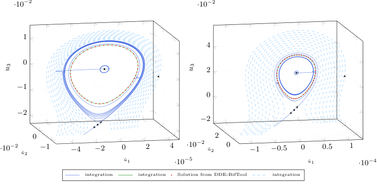
Figure 44: Comparing the computed homoclinic orbits in Eq. 110 with DDE-BifTool with the solutions obtained from numerical simulation with Julia. We see the numerical integrated solution going through all the red points from the solution from DDE-BifTool.
Refer to caption
Figure 45: Comparing the computed periodic orbits in Eq. 110 with DDE-BifTool with the solutions obtained from numerical simulation with Julia. We see the numerical integrated solution going through all the red points from the solution from DDE-BifTool.

10.18.1 Loading necessary Julia packages

We start by loading the necessary Julia packages. Compared with the previous demonstrations, we also need to load the Julia package Symbolics.jl [21] to differentiate the activation functions f1,f2,f3f_{1},f_{2},f_{3}.

10.18.2 Define system

Next we define the system to be integrated, a system to approximate the reverse flow, and also an allocating version used for stability calculations. Note that we need the Julia Symbolics.jl to differentiate the activation functions.

10.18.3 Function for creating streamlines plot

To obtain an impression of the flow near transcritical Bogdanov–Takens point, we create a streamlines function. This is particularly useful for seeing the flow around the stable manifold of the saddle-note.

10.18.4 Create figure with several axes

We create a figure containing multiple axis in which we will plot the homoclinic, periodic orbits, and the left and right-hand sides of Eq. 116.

10.18.5 Define parameters, equilibria

We define parameters located on the continued homoclinic branch with DDE-BifTool. Then calculate the equilibria points in Eq. 109 near the transcritical Bogdanov–Takens point.

10.18.6 Plot equilibria and homoclinic orbit

By plotting the homoclinic orbit obtained with DDE-BifTool located at parameter values

(α1,α2)=(−0.001724521613831,0.001344362436730),(\alpha_{1},\alpha_{2})=(-0.001724521613831,0.001344362436730),

we can compare with the numerical simulations. As in the analysis with DDE-BifTool, we rotate the coordinates of the solutions to visualize the solutions in phase-space.

10.18.7 Leading eigenvectors

Next, we calculate and plot the leading eigenvectors of the characteristic matrix at the saddle-node bifurcation point.

10.18.8 Define callback

Since we are only interested in the flow near the equilibria points, we create a continuous callback to ensure the orbits do not become too large.

10.18.9 Integrate the system at homoclinic orbits I

Now we define the problem to be integrated and choose the algorithm to be used. Then we integrate the system for a range of initial history functions using the function

streamlines}. Next, we integrate the system near
the inner equilibrium, i.e., the equilibrium inside the homoclinic orbit. This
equilibria should be an unstable spiral. We show the first and last part
of the obtained solutions. We see that the last part of the integrated solutions
completely overlap the homoclinic solution obtained with \DDEBIFTOOL.
\inputminted[firstline=142, lastline=165]
julia\pathToJuliaFiles/triNeuralBAMNetworkModel_simulation_article.jl

10.18.10 Add arrows on solutions

Lastly, we add arrows to the obtained solutions and redraw the equilibria.

We should now obtain an interactive figure similar to the left figure in Fig. 44.

10.18.11 Simulation near stable periodic orbit I

The code for numerical simulation near the second homoclinic orbit, see the right plot in Fig. 44, is not included here.

To show by integration the existence of a stable periodic orbit, we first located a periodic orbit in DDE-BifTool. This can be done by continuing a branch of periodic orbits emanating from a point on the continued Hopf curves. Then we load the profiles of the periodic orbits into Julia. We perform two simulations. For the first we integrate with a constant history function equal to a point inside the periodic orbit. The second simulation starts from the unstable eigenvector of the characteristic matrix calculated above.

After running the above code, we should obtain a similar plot as in Fig. 45.

10.18.12 Stability of the center manifold

To confirm Section 10 numerically, we consider again Eqs. 119 and 120. The code below plots the left and right-hand sides of Eq. 116. We see in Fig. 46 that there are two points of intersection.

Figure 46: Plot of the left and right-hand sides of Eq. 116. Points of intersection are candidates for the center manifold to lose its stability.

Using the function roots} from the package IntervalRootFinding.jl we search for points of intersection.

In the Julia output we obtain

7-element Vector{Root{Interval{Float64}}}:
Root([13.2309, 13.231], :unique)
Root([19.2374, 19.2375], :unique)
Root([19.7337, 19.7338], :unknown)
Root([6.00301, 6.00302], :unique)
Root([8.33333, 8.33334], :unknown)
Root([13.5353, 13.5354], :unknown)
Root([5.75402, 5.75403], :unknown)
Root([8.33333, 8.33334], :unknown)

Note that, since there are multiple discontinuities, there are many unknown solutions returned. We extract the unique solutions from the list of solutions and test if these provide solutions to the characteristic equation.

In the Julia output we obtain

The centermanifold is locally attractive for 0 < τ < 13.230934887939895.
Figure 47: Plot of the leading eigenvalues at the analytically derived transcritical Bogdanov–Takens point with τ=13.230934887939895\tau=13.230934887939895 and ω=ω⁡(τ)\omega=\omega(\tau) from Eq. 118. At this point there are four eigenvalues on the imaginary axis. For τ>13.230934887939895\tau>13.230934887939895 the center manifold is locally unstable.

10.18.13 Calculate and plot stability at Bogdanov–Takens point

We finish this demonstration by confirming the stability of the transcritical Bogdanov–Takens point at τ=13.230934887939895\tau=13.230934887939895 obtained in the previous section. In Fig. 47 we have plotted the eigenvalues. We indeed see that at τ=13.230934887939895\tau=13.230934887939895 the center manifold loses stability. Lastly, we also verified in the code below that the eigenvalues with positive imaginary part on the imaginary axis is approximately equal to the expression for ω\omega obtained in Eq. 118.

References for main text and supplement

  • [1] L. Benet and D. P. Sanders, IntervalRootFinding.jl. https://github.com/JuliaIntervals/IntervalRootFinding.jl, 2021.
  • [2] M. M. Bosschaert, S. G. Janssens, and Yu. A. Kuznetsov, Switching to nonhyperbolic cycles from codimension two bifurcations of equilibria of delay differential equations, SIAM J. Appl. Dyn. Syst., 19 (2020), pp. 252–303, https://doi.org/10.1137/19M1243993.
  • [3] M. M. Bosschaert and Yu. A. Kuznetsov, Interplay between normal forms and center manifold reduction for homoclinic predictors near bogdanov-takens bifurcation, 2021, https://arxiv.org/abs/arXiv:2109.12570.
  • [4] H. W. Broer, F. Dumortier, S. J. van Strien, and F. Takens, Structures in dynamics, vol. 2 of Studies in Mathematical Physics, North-Holland Publishing Co., Amsterdam, 1991. Finite-dimensional deterministic studies.
  • [5] P. Clément, O. Diekmann, M. Gyllenberg, H. J. A. M. Heijmans, and H. R. Thieme, Perturbation theory for dual semigroups. I. the sun-reflexive case, Math. Ann., 277 (1987), pp. 709–725, https://doi.org/10.1007/BF01457866.
  • [6] P. Clément, O. Diekmann, M. Gyllenberg, H. J. A. M. Heijmans, and H. R. Thieme, Perturbation theory for dual semigroups. II. time-dependent perturbations in the sun-reflexive case, Proc. Roy. Soc. Edinburgh Sect. A, 109 (1988), pp. 145–172, https://doi.org/10.1017/S0308210500026731.
  • [7] P. Clément, O. Diekmann, M. Gyllenberg, H. J. A. M. Heijmans, and H. R. Thieme, Perturbation theory for dual semigroups. III. nonlinear Lipschitz continuous perturbations in the sun-reflexive case, in Volterra integrodifferential equations in Banach spaces and applications (Trento, 1987), vol. 190 of Pitman Res. Notes Math. Ser., Longman Sci. Tech., Harlow, 1989, pp. 67–89.
  • [8] P. Clément, O. Diekmann, M. Gyllenberg, H. J. A. M. Heijmans, and H. R. Thieme, Perturbation theory for dual semigroups. IV. the intertwining formula and the canonical pairing, in Semigroup Theory and Applications (Trieste, 1987), vol. 116 of Lecture Notes in Pure and Appl. Math., Dekker, New York, 1989, pp. 95–116.
  • [9] V. De Witte, F. Della Rossa, W. Govaerts, and Yu. A. Kuznetsov, Numerical periodic normalization for codim 2 bifurcations of limit cycles: computational formulas, numerical implementation, and examples, SIAM J. Appl. Dyn. Syst., 12 (2013), pp. 722–788, https://doi.org/10.1137/120874904.
  • [10] V. De Witte, W. Govaerts, Yu. A. Kuznetsov, and H. G. E. Meijer, Analysis of bifurcations of limit cycles with Lyapunov exponents and numerical normal forms, Phys. D, 269 (2014), pp. 126–141, https://doi.org/10.1016/j.physd.2013.12.002.
  • [11] O. Diekmann and M. Gyllenberg, Abstract delay equations inspired by population dynamics, in Functional Analysis and Evolution Equations, Birkhäuser, 2008, pp. 187–200, https://doi.org/10.1007/978-3-7643-7794-6_12.
  • [12] O. Diekmann and M. Gyllenberg, Equations with infinite delay: blending the abstract and the concrete, J. Differential Equations, 252 (2012), pp. 819–851, https://doi.org/10.1016/j.jde.2011.09.038.
  • [13] O. Diekmann, S. A. van Gils, S. M. Verduyn Lunel, and H.-O. Walther, Delay Equations: Functional-, Complex-, and Nonlinear Analysis, Applied Mathematical Sciences, Springer, 1995, https://doi.org/10.1007/978-1-4612-4206-2.
  • [14] K. Dijkstra, S. A. van Gils, S. G. Janssens, Yu. A. Kuznetsov, and S. Visser, Pitchfork-Hopf bifurcations in 1D neural field models with transmission delays, Phys. D, 297 (2015), pp. 88–101, https://doi.org/10.1016/j.physd.2015.01.004.
  • [15] T. Dong and X. Liao, Bogdanov-Takens bifurcation in a tri-neuron BAM neural network model with multiple delays, Nonlinear Dynam., 71 (2013), pp. 583–595, https://doi.org/10.1007/s11071-012-0683-9.
  • [16] K. Engelborghs, T. Luzyanina, and D. Roose, Numerical bifurcation analysis of delay differential equations using DDE-BIFTOOL, ACM Trans. Math. Software, 28 (2002), pp. 1–21, https://doi.org/10.1145/513001.513002.
  • [17] T. Faria and L. T. Magalhães, Normal forms for retarded functional-differential equations and applications to Bogdanov-Takens singularity, J. Differential Equations, 122 (1995), pp. 201–224, https://doi.org/10.1006/jdeq.1995.1145.
  • [18] T. Faria and L. T. Magalhães, Normal forms for retarded functional differential equations with parameters and applications to Hopf bifurcation, Journal of differential equations, 122 (1995), pp. 181–200, https://doi.org/10.1006/jdeq.1995.1144.
  • [19] F. Giannakopoulos and A. Zapp, Bifurcations in a planar system of differential delay equations modeling neural activity, Physica D: Nonlinear Phenomena, 159 (2001), pp. 215–232.
  • [20] W. J. F. Govaerts, Numerical Methods for Bifurcations of Dynamical Equilibria, Society for Industrial and Applied Mathematics, Philadelphia, PA, 2000, https://doi.org/10.1137/1.9780898719543.
  • [21] S. Gowda, Y. Ma, A. Cheli, M. Gwóźzdź, V. B. Shah, A. Edelman, and C. Rackauckas, High-performance symbolic-numerics via multiple dispatch, ACM Commun. Comput. Algebra, 55 (2022), p. 92–96, https://doi.org/10.1145/3511528.3511535, https://doi.org/10.1145/3511528.3511535.
  • [22] S. G. Janssens, On a Normalization Technique for Codimension Two Bifurcations of Equilibria of Delay Differential Equations, master’s thesis, Utrecht University, The Netherlands, 2010, https://dspace.library.uu.nl/handle/1874/312252. Corrections and updates are available via http://sebastiaanjanssens.nl/pdf/normalization.pdf.
  • [23] S. G. Janssens, A class of abstract delay differential equations in the light of suns and stars, Jan. 2019, https://arxiv.org/abs/1901.11526.
  • [24] W. Jiang and Y. Yuan, Bogdanov–Takens singularity in van der Pol’s oscillator with delayed feedback, Physica D: Nonlinear Phenomena, 227 (2007), pp. 149–161.
  • [25] J. Jiao and C. Chen, Bogdanov–Takens bifurcation analysis of a delayed predator-prey system with double allee effect, Nonlinear Dynamics, 104 (2021), pp. 1697–1707, https://doi.org/10.1007/s11071-021-06338-x, https://doi.org/10.1007/s11071-021-06338-x.
  • [26] H. B. Keller, Lectures on Numerical Methods in Bifurcation Problems, vol. 79 of Tata Institute of Fundamental Research Lectures on Mathematics and Physics, Published for the Tata Institute of Fundamental Research, Bombay; by Springer-Verlag, Berlin, 1987. With notes by A. K. Nandakumaran and Mythily Ramaswamy.
  • [27] Yu. A. Kuznetsov, Numerical normalization techniques for all codim 2 bifurcations of equilibria in ODEs, SIAM Journal on Numerical Analysis, 36 (1999), pp. 1104–1124, https://doi.org/10.1137/S0036142998335005.
  • [28] Yu. A. Kuznetsov, Practical computation of normal forms on center manifolds at degenerate Bogdanov–Takens bifurcations, International Journal of Bifurcation and Chaos, 15 (2005), pp. 3535–3546.
  • [29] Yu. A. Kuznetsov, W. Govaerts, E. J. Doedel, and A. Dhooge, Numerical periodic normalization for codim 1 bifurcations of limit cycles, SIAM J. Numer. Anal., 43 (2005), pp. 1407–1435, https://doi.org/10.1137/040611306.
  • [30] C. Rackauckas and Q. Nie, Differentialequations.jl–a performant and feature-rich ecosystem for solving differential equations in julia, Journal of Open Research Software, 5 (2017).
  • [31] S. Ruan, On the zeros of a third degree exponential polynomial with applications to a delayed model for the control of testosterone secretion, Mathematical Medicine and Biology, 18 (2001), pp. 41–52, https://doi.org/10.1093/imammb/18.1.41, https://doi.org/10.1093%2Fimammb%2F18.1.41.
  • [32] G. Samaey, K. Engelborghs, and D. Roose, Numerical computation of connecting orbits in delay differential equations, Numer. Algorithms, 30 (2002), pp. 335–352, https://doi.org/10.1023/A:1020102317544, https://doi-org.proxy.library.uu.nl/10.1023/A:1020102317544.
  • [33] D. P. Sanders, L. Benet, Lucaferranti, Krish Agarwal, B. Richard, J. Grawitter, Eeshan Gupta, M. Forets, M. F. Herbst, Yashrajgupta, E. Hanson, Braam Van Dyk, C. Rackauckas, Rushabh Vasani, S. Miclu t , a-Câmpeanu, Sheehan Olver, T. Koolen, C. Wormell, Favio André Vázquez, G. Dalle, J. Sarnoff, J. TagBot, K. O’Bryant, K. Carlsson, M. Piibeleht, M. Giordano, , Reno, R. Deits, T. Holy, and Venkateshprasad, Juliaintervals/intervalarithmetic.jl: v0.20.6, 2022, https://doi.org/10.5281/ZENODO.6569509, https://zenodo.org/record/6569509.
  • [34] J. Sieber, Local bifurcations in differential equations with state-dependent delay, Chaos: An Interdisciplinary Journal of Nonlinear Science, 27 (2017), p. 114326, https://doi.org/10.1063/1.5011747, https://arxiv.org/abs/1705.07550.
  • [35] J. Sieber, K. Engelborghs, T. Luzyanina, G. Samaey, and D. Roose, DDE-BIFTOOL Manual - Bifurcation analysis of delay differential equations, June 2014, https://arxiv.org/abs/1406.7144.
  • [36] S. A. van Gils, S. G. Janssens, Yu. A. Kuznetsov, and S. Visser, On local bifurcations in neural field models with transmission delays, Journal of Mathematical Biology, 66 (2013), pp. 837–887, https://doi.org/10.1007/s00285-012-0598-6, https://arxiv.org/abs/1209.2849.