A unified model of inflation and dark energy based on the holographic spacetime foam

Recent cosmological observations indicate that the universe is currently experiencing an accelerated expansion Riess et al. 1998; Perlmutter et al. 1999; Spergel et al. 2003; Tegmark et al. 2004. This fact can be attributed to the existence of some form of energy (dubbed dark energy) with negative pressure. Our unawareness of the nature of dark energy is certainly at the root of one of the greatest unknowns in theoretical physics: the cosmological constant problem Weinberg 1989. On the other hand, it is widely accepted today that the very early universe underwent a period of quasi-exponential expansion called inflation, which can address many of the problems of the standard Big Bang cosmology Guth 1981; Starobinsky 1979; Kazanas 1980; Sato 1981; Linde 1982; Albrecht and Steinhardt 1982.

Both expansion epochs may be traced to a common cause by interpreting dark energy as a dynamical scalar field (the inflaton) that slowly rolls down its potential to drive inflation in the early universe and finally resembles a cosmological constant at the present time, at a much lower energy scale. Depending on the shape of the potential, the field will end up oscillating about a minimum (as in the model presented in this paper) or rolling down an infinite tail as quintessence. The latter scenario is called quintessential inflation Peebles and Vilenkin 1999.

Another chance of uncovering the nature of dark energy may be found in the structure of spacetime itself. Due to its quantum nature, spacetime is foamy on scales of the order of the Planck length Misner et al. 1973. The quantum fluctuations of the metric are responsible for a perpetual change in the geometry of spacetime, and consequently, any measurement of space and time intervals acquires some uncertainty. In a region of spatial extent $L$, this uncertainty is given by the Károlyházy relation Karolyhazy 1966, which was derived independently by other authors Sasakura 1999; Ng and Van Dam 1994; Christiansen et al. 2006; Arzano et al. 2007:

$$\delta L\sim L_{p}^{2/3}L^{1/3},$$

(1)

where $L_{p}$ is the Planck length. Note that $\delta L\sim L$ precisely at the Planck scale. This picture of the small scale structure of spacetime is called spacetime foam. An appealing idea that has been proposed is that the energy density associated to the spacetime foam is the one that drives both the early and late expansions of the universe Ng 2021.

The Károlyházy uncertainty relation (1) is closely related to the holographic principle ’t Hooft 1993; Susskind 1995, as it establishes a connection between the ultraviolet ($\delta L$) and infrarred ($L$) cut-off scales of the system. Indeed, expression (1) is also known as the holographic spacetime foam model, as it suggests that the number of degrees of freedom or bits of information in that region is proportional to its surface area: $\left(L/\delta L\right)^{3}\propto L^{2}$. The ultraviolet cut-off scale is related to the energy density of the vacuum, and one is led to a holographic dark energy of the form

$$\rho\sim\frac{1}{L_{p}^{2}L^{2}}\,.$$

(2)

The usual approach in holographic dark energy models is to propose an ansatz for the infrarred cut-off $L$ (some natural choices are the Hubble radius Hsu 2004; Zimdahl and Pavon 2007, the event horizon Li 2004, the age of the universe Cai 2007 and the Ricci length Duran and Pavon 2011) and combine equation (2) with the Friedmann equation in order to extract the Hubble rate as a function of time. Then, one can see whether this particular choice leads to an accelerated expansion, and also constrain the model with the observational data. While these models have been intensively applied to the late universe (see del Campo et al. 2011 for a review), only a few authors have extended these ideas to the early universe (for instance, see Nojiri et al. 2019).

Finally, and more on the line of thought of this work, there have been several studies aimed at establishing a connection between holographic dark energy and scalar field models Zhang 2010; Karami and Fehri 2010; Cui et al. 2010; Sheykhi et al. 2010, although the explicit reconstruction of the scalar field potential has proved to be challenging (however, see Sheykhi 2011; Granda and Oliveros 2009).

In this paper, I present a unified model of inflation and dark energy in which the scalar potential is reconstructed by making a specific ansatz for the field in the cosmological equations. This ansatz will be rooted at the holographic model of spacetime foam.

This letter is structured as follows: in section 2, I expose the main idea behind the construction of the inflaton potential. This idea is applied in section 3 under the assumption that the scalar field is real. In this case, the potential obtained is not satisfactory. The calculation is redone in section 4 for a complex scalar field, obtaining a family of acceptable potentials. In section 5, I pick up the potential that has direct connection with the spacetime foam and I discuss some of its properties. Finally, some concluding remarks are made in section 6.

Natural units ($c=\hbar\equiv 1$) are used throughout the letter. In particular, this implies that Newton’s gravitational constant is given by $G=L_{p}^{2}=M_{p}^{-2}$, where $M_{p}$ is the Planck mass.

Regardless of the initial field configuration in the patch of the universe that is going to inflate, the field evolves under the influence of a potential $V\left(\phi\right)$. The Friedmann and Klein-Gordon equations in a spatially flat Friedmann-Lemaître-Robertson-Walker (FLRW) universe establish a correspondence between the potential and a homogeneous function of time $\phi\left(t\right)$. Therefore, one can obtain the scalar potential by imposing that a particular $\phi_{s}\left(t\right)$ is an exact solution to these equations (the subscript $s$ stands for solution). For instance, $V\left(\phi\right)$ could be determined by imposing that $\phi_{s}\left(t\right)\propto H\left(t\right)$ is a solution to the equations (here and henceforth, $H$ denotes the Hubble rate). Whatever our ansatz is, $\phi_{s}\left(t\right)$ is not the actual inflaton field $\phi\left(t,\vec{x}\right)$ in the universe, but just a tool to determine the potential. Indeed, a natural initial state for the field is arbitrary and inhomogeneous. Since $\phi\left(t=0,\vec{x}\right)\neq\phi_{s}\left(t=0\right)$ and $\dot{\phi}\left(t,\vec{x}\right)\neq\dot{\phi}_{s}\left(t=0\right)$, the inflaton field would simply end up settling in the vacuum of the potential, possibly resembling the cosmological constant.

Here we will obtain a family of scalar field potentials by considering the simplest ansatz with dimensions of energy that one can make out of $M_{p}$ and $H$:

$$\phi_{s}\left(H\right)=AM_{p}^{\gamma}H^{1-\gamma},$$

(3)

where $A$ is a dimensionless constant and $\gamma$ is a generic exponent that will label the different elements of the family of solutions. Some of them will not only have the right shape to allow for inflation in the early universe and cosmological constant at the present time, but also a connection with the spacetime foam, as we point out now.

Note that ansatz (3) for $\gamma=2/3$ is essentially the inverse of the Károlyházy uncertainty relation (1) evaluated at the Hubble scale. One can show that $1/\delta L$ is proportional to the energy of the spacetime foam inside the Hubble horizon. The classical energy density associated to the metric fluctuations is given by Maziashvili 2006

$$\rho_{foam}\sim\frac{1}{L_{p}^{2/3}L^{10/3}},$$

(4)

and although this expression was derived in Minkowski spacetime, we will assume that the powers of $L_{p}$ and $L$ remain unchanged in a spatially flat FLRW universe. If the scale $L$ in equation (4) is chosen to be the Hubble radius, the classical energy of the spacetime foam in that volume is

$$E_{foam}\sim M_{p}^{2/3}H^{1/3}.$$

(5)

This expression for the energy can also be derived from the Margolus-Levitin theorem in quantum computation Margolus and Levitin 1998. The dynamical evolution of any physical system can be thought of as a succession of orthogonal quantum states, and each step between consecutive states can be understood as an elementary operation. It can be easily shown that each of these steps takes at least time $\delta t\sim E^{-1}$, where $E$ is the average energy of the system. Therefore, $E\sim\delta t^{-1}$, which yields expression (5) if we impose that $\delta t$ corresponds to the uncertainty given by the Károlyházy relation (1) evaluated at the Hubble scale.

The simplest possibility is to consider a real scalar field. The first Friedmann equation and the Klein-Gordon equation read

$$H^{2}=\frac{8\pi}{3M_{p}^{2}}\left[\frac{\dot{\phi}^{2}}{2}+V\left(\phi\right)\right],$$

(6)

$$\ddot{\phi}+3H\dot{\phi}+\frac{dV}{d\phi}=0.$$

(7)

Taking the time derivative of (6) and combining it with (7) yields

$$\dot{H}=-\frac{4\pi}{M_{p}^{2}}\dot{\phi}^{2}.$$

(8)

Since $\phi=\phi\left(t\right)$ and $H=H\left(t\right)$, one can take $H=H\left(\phi\right)$. Taking this into account, and using equations (6) and (8), one can express $V\left(\phi\right)$ as

$$V\left(\phi\right)=\frac{M_{p}^{2}}{8\pi}\left[3H^{2}\left(\phi\right)-\frac{M_{p}^{2}}{4\pi}\left(\frac{dH}{d\phi}\right)^{2}\right]\,.$$

(9)

Now we determine $V\left(\phi\right)$ by imposing that $\phi=\phi_{s}\left(H\right)$, given by equation (3). Inverting to get $H\left(\phi\right)$ and substituting in (9) yields

$$V\left(\phi\right)=\frac{M_{p}^{\frac{2\left(1-2\gamma\right)}{1-\gamma}}}{8\pi A^{\frac{2}{1-\gamma}}}\left[3\phi^{\frac{2}{1-\gamma}}-\frac{M_{p}^{2}}{4\pi\left(1-\gamma\right)^{2}}\phi^{\frac{2\gamma}{1-\gamma}}\right]\,.$$

(10)

We further assume that $V\left(\phi\right)$ takes finite values for finite $\phi$. Together with the fact that the potential is real, this implies that the exponent $\frac{2\gamma}{1-\gamma}\equiv n$ is a natural number (if this is the case, the first exponent is also a natural number: $\frac{2}{1-\gamma}=n+2$). This means that $\gamma$ is quantized: $\gamma=\frac{n}{2+n}$. As shown in figures 1 and 2, the potential is either symmetric (if $n$ is even) or antisymmetric (if $n$ is odd). For $\gamma=0$, the potential is a parabola with its minimum at $\phi=0$, at a negative energy density.

In the case of the symmetric double-well potentials, note that the flatness around $\phi=0$ is controlled by $\gamma$. Note also that the minima are placed at negative values of the potential energy density. Therefore, none of them can be the actual potential for the inflaton. However, if one considers a complex scalar field, the potential contains an extra term related to the phase. This extra term can act as an uplifting term, so one can obtain vacua with positive cosmological constant in that case.

If we consider a complex field $\phi=\frac{\varphi}{\sqrt{2}}e^{i\frac{\beta}{\varphi_{v}}}$, where $\beta$ is the angular part of the field and $\varphi_{v}$ is the vacuum expectation value of the radial part, equations (6) and (8) read

$$H^{2}=\frac{8\pi}{3M_{p}^{2}}\left[\frac{\dot{\varphi}^{2}}{2}+\frac{\varphi^{2}\dot{\beta}^{2}}{2\varphi_{v}^{2}}+V\left(\varphi\right)\right],$$

(11)

$$\dot{H}=-\frac{4\pi}{M_{p}^{2}}\left(\dot{\varphi}^{2}+\frac{\varphi^{2}\dot{\beta}^{2}}{\varphi_{v}^{2}}\right).$$

(12)

Again, we assume that $\varphi$ is a function of $H$ and hence $H=H\left(\varphi\right)$. Combining equations (11) and (12), one gets

$$V\left(\varphi\right)=\frac{M_{p}^{2}}{8\pi}\left[3H^{2}\left(\varphi\right)-\frac{M_{p}^{2}}{4\pi}\left(\frac{dH}{d\varphi}\right)^{2}-\frac{\varphi^{2}\dot{\beta^{2}}}{\varphi_{v}^{2}\dot{\varphi}}\frac{dH}{d\varphi}\right]\,.$$

(13)

This potential has the same form as (9), except for the presence of a new term that contains the time derivative of the angular part of the field. Note that this extra term can be written as $-\frac{\varphi^{2}\dot{\beta^{2}}}{\varphi_{v}^{2}\dot{\varphi}^{2}}\dot{H}$, and this is always positive as $\dot{H}<0$ (see equation (12)). If the phase $\beta$ is chosen in such a way that

$$\dot{\beta}^{2}\propto\frac{dH^{-1}}{dt}\,,$$

(14)

that is, proportional to the slow-roll parameter $\epsilon$, the extra term is a constant that uplifts the potential found in the previous section. Note that this choice of $\beta$ is made at the same level as ansatz (3) for $\varphi$. The phase determined by equation (14), as well as any other $\beta$ that one could have come up with, is an exact solution of the equations of motion provided that the potential energy density is given by (13). Other choices of $\beta$ could also do the job of uplifting the potential by locally deforming it, but in these cases the deformation would not be uniform in $\varphi$. This uniformity condition is obviously not necessary to obtain a potential with the right properties to account for the expansion history of the universe, but let us focus on this possibility for simplicity. Making use of ansatz (14), the extra term in the potential is a positive constant with dimensions of energy squared: $-\frac{\varphi^{2}\dot{\beta^{2}}}{\varphi_{v}^{2}\dot{\varphi}}\frac{dH}{d\varphi}\equiv BM_{p}^{2}$, where $B>0$ is a dimensionless constant.

Now we impose that $\varphi=\varphi_{s}\left(H\right)=AM_{p}^{\gamma}H^{1-\gamma}$. Finding $H\left(\varphi\right)$ and substituting in (13), one gets the following potential:

$$V\left(\varphi\right)=\frac{M_{p}^{\frac{2\left(1-2\gamma\right)}{1-\gamma}}}{8\pi A^{\frac{2}{1-\gamma}}}\left[3\varphi^{\frac{2}{1-\gamma}}-\frac{M_{p}^{2}}{4\pi\left(1-\gamma\right)^{2}}\varphi^{\frac{2\gamma}{1-\gamma}}\right]+\frac{BM_{p}^{4}}{8\pi}\,.$$

(15)

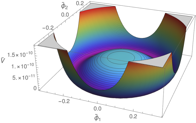
For the values of $\gamma$ corresponding to even $n=\frac{2\gamma}{1-\gamma}$, this is a Mexican-hat potential with the circle of minima at $\varphi=\varphi_{v}=M_{p}\sqrt{\frac{\gamma}{12\pi\left(1-\gamma\right)^{2}}}$. The vacuum energy density can be shown to be

$$V\left(\varphi_{v}\right)=-\frac{M_{p}^{2}m^{2}}{48\pi}+\frac{BM_{p}^{4}}{8\pi}\,,$$

(16)

where $m=f\left(\gamma\right)M_{p}$ is the mass of small radial fluctuations about the vacuum, i.e., the mass of the inflaton field. The function $f\left(\gamma\right)$ is given by

$$f\left(\gamma\right)=\left[\frac{\gamma^{\gamma}}{8^{1-\gamma}\times 12^{2\gamma-1}\pi\left(1-\gamma\right)^{1+\gamma}A^{2}}\right]^{\frac{1}{2\left(1-\gamma\right)}}.$$

(17)

We want the vacuum energy density (16) to be equal to the dark energy density today, namely, $\rho_{\Lambda}^{0}=\Omega_{\Lambda}^{0}\rho_{c}^{0}=\frac{3\Omega_{\Lambda}^{0}}{8\pi}H_{0}^{2}M_{p}^{2}$. This implies that

$$B=3\Omega_{\Lambda}^{0}\left(\frac{H_{0}}{M_{p}}\right)^{2}+\frac{1}{6}\left(\frac{m}{M_{p}}\right)^{2}\approx\frac{1}{6}\left(\frac{m}{M_{p}}\right)^{2}\,.$$

(18)

The first term is negligible, but its presence makes this choice of $B$ extremely fine-tuned. Evidently, since the model does not provide a fundamental explanation for it, the cosmological constant problem is not resolved. However, once this term is neglected, the approximate value of $B$ is arguably natural: condition (18) implies that the Hubble rate during inflation ($H_{I}$) is given by

$$H_{I}\approx\sqrt{\frac{8\pi}{3M_{p}^{2}}V\left(0\right)}=M_{p}\sqrt{\frac{B}{3}}\approx\frac{m}{3\sqrt{2}}\,.$$

(19)

This means that the Hubble radius during inflation is of the same order of magnitude as the Compton wavelength of the inflaton, which is the only fundamental length scale in the problem apart from the Planck length. Therefore, although the model requires fine-tuning to explain the exact value of the cosmological constant, it may not need it to account merely for its smallness.

As previously stated, the ansatz for the radial part of the scalar field can be interpreted as the energy of the spacetime foam inside the Hubble horizon if $\gamma=2/3$. Defining $\tilde{\varphi}\equiv\varphi/M_{p}$ and $\tilde{V}\equiv V/M_{p}^{4}$, and making use of (17) and (18), the potential (15) for $\gamma=2/3$ can be written as

$$\tilde{V}\left(\tilde{\varphi}\right)\approx\left(\frac{m}{M_{p}}\right)^{2}\left[\frac{\pi^{2}}{3}\left(\tilde{\varphi}^{6}-\frac{3}{4\pi}\tilde{\varphi}^{4}\right)+\frac{1}{48\pi}\right]\,.$$

(20)

With this potential, plotted in figure 3, ansatz (3) with $\gamma=2/3$ for $\varphi$ and ansatz (14) for $\beta$ are exact solutions of the equations of motion. This means that, until radiation and matter become important and influence the dynamics of the scalar field, $\varphi$ and $\beta$ would evolve as dictated by their corresponding ansätze as long as the initial conditions for both of them are exactly given by these expressions. However, we find it more natural to consider the possibility that the initial state is arbitrary and inhomogeneous, and that the scalar field is in different regions of the potential in different Hubble patches. In this case, $\varphi$ and $\beta$ will definitely not follow (3) and (14), as the evolution of the scalar field will proceed essentially as in a cosmological phase transition. As we will shortly see, a patch of the universe where the radial part of the scalar field starts out sufficiently close to $\varphi\left(t=0,\vec{x}\right)=0$ in potential (20) will undergo inflation. After that, the field will reach the circle of minima at $\varphi=\varphi_{v}$ and will start oscillating as dictated by the Friedmann and Klein-Gordon equations. Production of the standard model particles will then take place and the universe will be subsequently dominated by radiation and matter. In the long term, the residual vacuum energy (16) of the field will start dominating as a cosmological constant.

Let us note that, even if the initial conditions were those determined by the ansätze (3) and (14), quantum fluctuations on top of that state may spoil the subsequent expected evolution and yield a picture which would be similar to the one presented above.

The properties of the $\gamma=2/3$ potential (20) are studied quantitatively in the following subsections.

I have presented a novel approach to describe early inflation and the late time acceleration of the universe in a unified picture, in the sense that a single scalar potential can account for both cosmic eras. In this proposal, the potential is determined by imposing that a scalar field with a particular meaning is an exact solution to the Friedmann and Klein-Gordon equations in a spatially flat FLRW universe.

The ansatz for the scalar field has been associated with the energy of the spacetime foam inside the Hubble horizon. This correspondence leads to a potential that allows for more than enough inflation in the early universe, and it yields acceptable values for the inflationary observables. Demanding consistency with the observational data and imposing natural bounds on the parameters of the model, one gets the following estimate for the mass of the inflaton: $m\sim 10^{-5}M_{p}$. Moreover, the potential can also describe the current expansion of the universe as the field ends up at a circle of vacua at positive energy density given by (16), thus acting effectively as a cosmological constant. Although the model cannot justify the exact value of the vacuum energy, it predicts that it has to be much smaller than $M_{p}^{4}$ if one assumes that the Hubble radius during inflation is of the order of the Compton wavelength of the inflaton.

Remarkably, the requirement that the potential does not blow up for finite values of the field yields the quantization of $\gamma$. The particular solution $\gamma=2/3$ turns out to be special, because it is the one that minimizes the mass of the inflaton. Since this is precisely the solution with direct connection with the holographic model of spacetime foam, this might be regarded as an argument to strengthen our faith on the Károlyházy uncertainty relation.

I would like to express my sincere gratitude to Y. Jack Ng and Diego Pavón for their support and insightful words. I am also grateful to L.N. Granda, Thomas W. Kephart and Ahmad Sheykhi for useful comments.

References

- Riess et al. (1998) A. Riess et al., The Astrophysical Journal 116, 1009 (1998).
- Perlmutter et al. (1999) S. Perlmutter et al., The Astrophysical Journal 517, 565 (1999).
- Spergel et al. (2003) D. Spergel et al., The Astrophysical Journal Supplement Series 148, 175 (2003).
- Tegmark et al. (2004) M. Tegmark et al., Physical Review D 69 (2004), 10.1103/physrevd.69.103501.
- Weinberg (1989) S. Weinberg, Reviews of Modern Physics 61, 1 (1989).
- Guth (1981) A. Guth, Physical Review D 23, 347 (1981).
- Starobinsky (1979) A. Starobinsky, JETP Letters 30, 682 (1979).
- Kazanas (1980) D. Kazanas, The Astrophysical Journal 241, L59 (1980).
- Sato (1981) K. Sato, Monthly Notices of the Royal Astronomical Society 195, 467 (1981).
- Linde (1982) A. Linde, Physics Letters B 108, 389 (1982).
- Albrecht and Steinhardt (1982) A. Albrecht and P.J. Steinhardt, Physical Review Letters 48, 1220 (1982).
- Peebles and Vilenkin (1999) P.J.E. Peebles and A. Vilenkin, Phys. Rev. D 59, 063505 (1999).
- Misner et al. (1973) C. W. Misner, K. S. Thorne, and J. A. Wheeler, Gravitation (W.H. Freeman and Company, 1973).
- Karolyhazy (1966) F. Karolyhazy, II Nuovo Cimento A 42, 390 (1966).
- Sasakura (1999) N. Sasakura, Progress of Theoretical Physics 102, 169 (1999).
- Ng and Van Dam (1994) Y. Ng and H. Van Dam, Modern Physics Letters A 9, 335 (1994).
- Christiansen et al. (2006) W.A. Christiansen, Y.J. Ng, and H. van Dam, Physical Review Letters 96, 051301 (2006).
- Arzano et al. (2007) M. Arzano, T. Kephart, and Y. Ng, Physics Letters B 649, 243 (2007).
- Ng (2021) Y. Ng, Symmetry 13 (2021), https://doi.org/10.3390/sym13030435.
- ’t Hooft (1993) G. ’t Hooft, (1993), gr-qc/9310026 .
- Susskind (1995) L. Susskind, Journal of Mathematical Physics 36, 6377 (1995).
- Hsu (2004) S. Hsu, Physics Letters B 594, 13 (2004).
- Zimdahl and Pavon (2007) W. Zimdahl and D. Pavon, Classical and Quantum Gravity 24, 5461 (2007).
- Li (2004) M. Li, Physics Letters B 603, 1 (2004).
- Cai (2007) R.-G. Cai, Physics Letters B 657, 228 (2007).
- Duran and Pavon (2011) I. Duran and D. Pavon, Journal of Physics: Conference Series 314, 012058 (2011).
- del Campo et al. (2011) S. del Campo, J.C. Fabris, R. Herrera, and W. Zimdahl, Physical Review D 83, 123006 (2011).
- Nojiri et al. (2019) S. Nojiri, S. Odintsov, and E. Saridakis, Physics Letters B 797, 134829 (2019).
- Zhang (2010) X. Zhang, Physics Letters B 682, 1 (2010).
- Karami and Fehri (2010) K. Karami and J. Fehri, Physics Letters B 684, 61 (2010).
- Cui et al. (2010) J. Cui, L. Zhang, J. Zhang, and X. Zhang, Chin. Phys. B 19, 019802 (2010).
- Sheykhi et al. (2010) A. Sheykhi, A. Bagheri, and M. Yazdanpanah, JCAP 09, 017 (2010).
- Sheykhi (2011) A. Sheykhi, Physical Review D 84, 107302 (2011).
- Granda and Oliveros (2009) L. Granda and A. Oliveros, Physics Letters B 671, 199 (2009).
- Maziashvili (2006) M. Maziashvili, International Journal of Modern Physics D 16, 1531 (2006).
- Margolus and Levitin (1998) N. Margolus and L. B. Levitin, Physica D 120, 188 (1998).
- Akrami et al. (2020) Y. Akrami et al., Astron. Astrophys. 641, A10 (2020).