Time Will Tell: New Outlooks and A Baseline for Temporal Multi-View 3D Object Detection
Abstract
While recent camera-only 3D detection methods leverage multiple timesteps, the limited history they use significantly hampers the extent to which temporal fusion can improve object perception. Observing that existing works’ fusion of multi-frame images are instances of temporal stereo matching, we find that performance is hindered by the interplay between 1) the low granularity of matching resolution and 2) the sub-optimal multi-view setup produced by limited history usage. Our theoretical and empirical analysis demonstrates that the optimal temporal difference between views varies significantly for different pixels and depths, making it necessary to fuse many timesteps over long-term history. Building on our investigation, we propose to generate a cost volume from a long history of image observations, compensating for the coarse but efficient matching resolution with a more optimal multi-view matching setup. Further, we augment the per-frame monocular depth predictions used for long-term, coarse matching with short-term, fine-grained matching and find that long and short term temporal fusion are highly complementary. While maintaining high efficiency, our framework sets new state-of-the-art on nuScenes, achieving first place on the test set and outperforming previous best art by 5.2% mAP and 3.7% NDS on the validation set. Code will be released here: https://github.com/Divadi/SOLOFusion.
1 Introduction
Recent advances in camera-only 3D detection have alleviated monocular ambiguities by leveraging a short history. Despite their improvements, these outdoor works neglect the majority of past observations, limiting their temporal fusion to a few frames in a short 2-3 second window. These long-term past observations are critical for better depth estimation - the main bottleneck of camera-only works.
Although existing methods aggregate temporal features differently, in essence, these works all consider regions in 3D space and consider image features corresponding to these hypothesis locations from multiple timesteps. Then, they use this temporal information to determine the occupancy of or the existence of an object at those regions. As such, these works are instances of temporal stereo matching. To quantify the quality of multi-view (temporal) depth estimation possible in these methods, we define localization potential at a 3D location as the magnitude of the change in the source-view projection induced by a change in depth in the reference view. As shown in Figure 1, a larger localization potential causes depth hypotheses Yao et al. 2018 for a reference view pixel to be projected further apart, giving them more distinct source view features. Then, the correct depth hypothesis with a stronger match with the source view feature can more easily suppress incorrect depth hypotheses with clearly unrelated features, allowing for more accurate depth estimation.
We evaluate the localization potential in driving scenarios and find that only using a few recent frames heavily limits the localization potential, and thus the depth estimation potential, of existing methods. Distinct from the intuition in both indoor works, which select frames with above a minimum translation and rotation (Hou et al. 2019; Sun et al. 2021), and outdoor works, which often empirically select a single historical frame (Huang & Huang 2022; Wang et al. 2022b; Liu et al. 2022b), we find that the optimal rotation and temporal difference between the reference and source frame varies significantly over different pixels, depths, cameras, and ego-motion. Hence, it is necessary to utilize many timesteps over a long history for each pixel and depth to have access to a setup that maximizes its localization potential. Further, we find that localization potential is not only decreased by fewer timesteps but is also hurt by the lower image feature resolution used in existing methods. Both factors significantly hinder the benefits of temporal fusion in prior works.
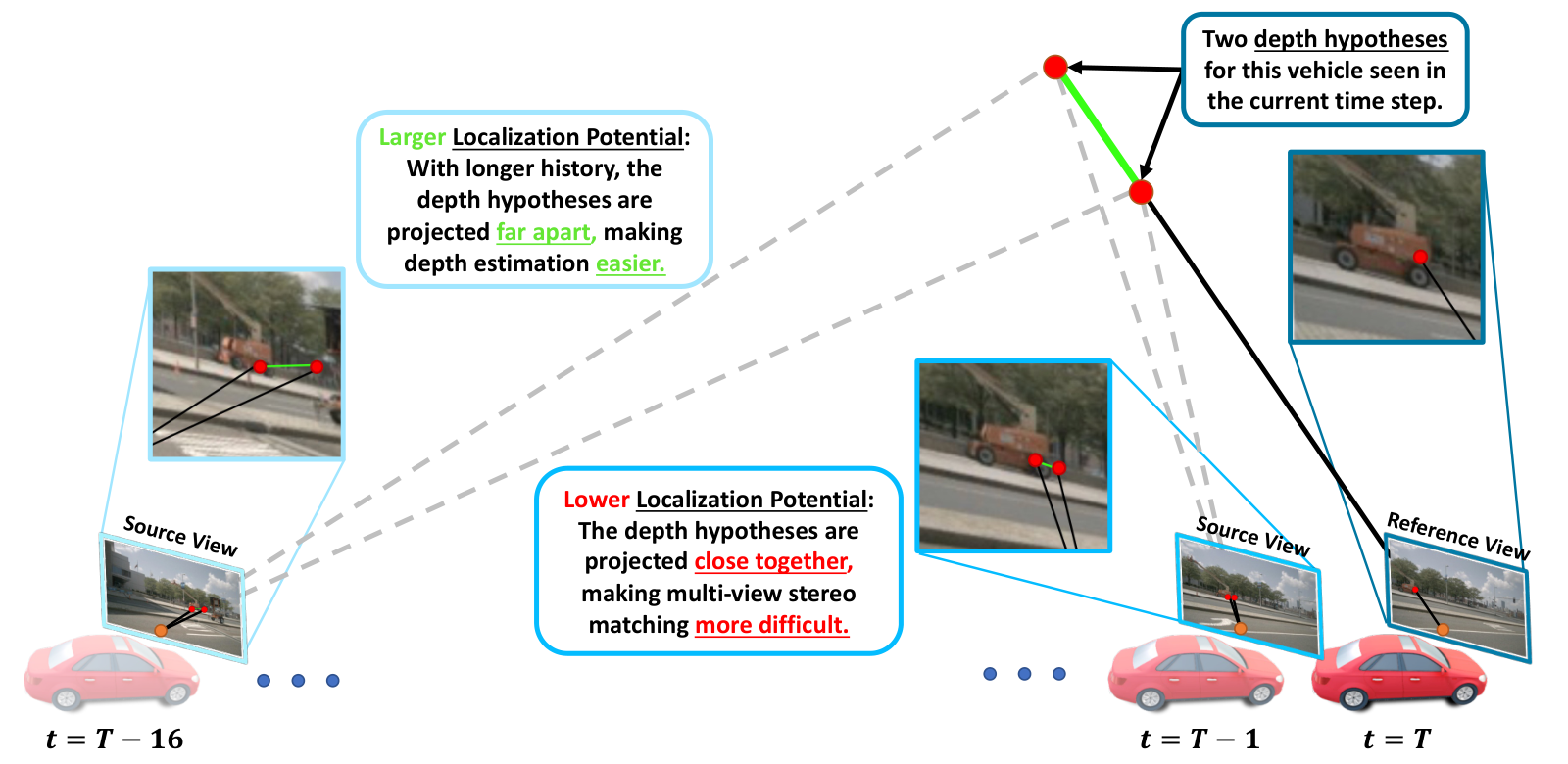
We verify our theoretical analysis by designing a model that naturally follows from our findings. Although existing methods’ usage of low-resolution image feature maps for multi-view stereo limits matching quality, our proposed long-term temporal fusion’s dramatic increase in localization potential can offset this limitation. Our model adopts the coarse but efficient low-resolution feature maps and leverages a 16-frame BEV cost volume. We find that such a framework already outperforms prior-arts, highlighting the significant gap in utilizing temporal information in existing literature. We extend our model by further exploiting short-term temporal fusion with an efficient sampling module, replacing monocular depth priors in the 16-frame BEV cost volume with a two-view depth prior. This time offsetting the temporal decrease in localization potential with an increase in feature map resolution, we observe a further boost in performance, demonstrating that short-term and long-term temporal fusion are highly complementary. Our main contributions are as follows:
- •
We define localization potential to measure the ease of multi-view depth estimation and use it to theoretically and empirically demonstrate that the optimal rotation and temporal difference between reference and source cameras for multi-view stereo varies significantly over pixels and depths. This runs contrary to intuition in existing works that impose a minimum view change threshold or empirically search for a single past frame to fuse.
- •
We verify our theoretical analysis by designing a model, SOLOFusion, that leverages both ShOrt-term, high-resolution and LOng-term, low-resolution temporal stereo for depth estimation. Critically, we are the first, to the best of our knowledge, to balance the impacts of spatial resolution and temporal difference on localization potential and use it to design an efficient but strong temporal multi-view 3D detector in the autonomous driving task.
- •
Our framework significantly outperforms state-of-the-art methods in utilizing temporal information, demonstrating considerable improvement in mAP and mATE over a strong non-temporal baseline as shown in Figure 2. SOLOFusion achieves first on the nuScenes test set and outperforms previous best art by 5.2% mAP and 3.7% NDS on the validation set.
2 Related Work
2.1 Single-View Camera-Only 3D Object Detection
Many single-view methods use mature 2D CNNs and predict 3D boxes from the image (Mousavian et al. 2017; Brazil & Liu 2019; Qin et al. 2019; Xu & Chen 2018; Zhou et al. 2019). Some works leverage CAD models (Liu et al. 2021; Manhardt et al. 2019; Barabanau et al. 2020) while others set prediction targets as keypoints (Li et al. 2022e; Zhang et al. 2021) or disentangled 3D parameters (Simonelli et al. 2019; Wang et al. 2021). Another line of work predicts in 3D, using monocular depth prediction networks (Fu et al. 2018; Godard et al. 2017) to generate pseudo-LiDAR (Wang et al. 2019; Weng & Kitani 2019) and applying LiDAR-based 3D detection frameworks. Our paper addresses monocular 3D ambiguity through temporal fusion and is perpendicular to these works.
2.2 Multi-View Camera-only 3D Object Detection
Most multi-camera works operate in 3D space. Following LSS (Philion & Fidler 2020), some methods (Reading et al. 2021; Huang et al. 2021; Li et al. 2022a) predict a distribution over depth bins and generate a point cloud with probability-weighted image features to be used for BEV detection. Followup works (Liu et al. 2022c; Li et al. 2022c) speed up voxelization and introduce depth supervision (Li et al. 2022c). Another branch of works follow DETR3D Wang et al. 2022c and adopt a queries. These works use object queries (Wang et al. 2022c; Liu et al. 2022a; Chen et al. 2022; Jiang et al. 2022) or BEV grid queries (Li et al. 2022d) and project them to get image features.
Recent works extend LSS and query frameworks to process several frames. Most LSS methods align and concatenate volumes from multiple timesteps (Huang & Huang 2022; Li et al. 2022c; Li et al. 2022a), and query-based methods sample from past images through projection (Chen et al. 2022; Jiang et al. 2022) or attention (Liu et al. 2022b; Li et al. 2022d). However, these methods demonstrate limited improvement from temporal fusion. Most of these works fuse multi-frame features at low resolution and use a limited number of timesteps over a short time window - both factors that we find severely decrease localization potential. In our work, we quantify these limitations and propose a strong framework that explicitly considers the relationship between spatial resolution and temporal history.
2.3 Multi-View Stereo
Recent multi-view stereo focus on using depth maps (Kang et al. 2001) and 3D volumes (Kutulakos & Seitz 2000) to conduct depth, mesh, and point-cloud reconstruction tasks. Several methods (Galliani et al. 2015; Ji et al. 2017) use a depth map fusion algorithm for large-scale scenes. Other works (Kar et al. 2017; Yao et al. 2018; Yang et al. 2020; Zbontar et al. 2016; Yao et al. 2019) generate a 3D volume by scattering pixel features to the 3D grid and estimating occupancy probability or cost for each voxel. A few methods apply multi-view stereo works to 3D detection. DfM (Wang et al. 2022a) generates a plane-sweep volume from consecutive frames. STS (Wang et al. 2022d) uses spatially-increasing discretization (SID) depth bins (Fu et al. 2018) for stereo matching, and BEVStereo (Li et al. 2022b) adapts MaGNet (Bae et al. 2022) and dynamically selects candidates for iterative multi-view matching.
Although these methods demonstrate further improvement, the short history they use for detection limits their gain from temporal fusion as shown in Figure 2. We formulate and analyze the connection between temporal camera-only 3D detection and multi-view stereo and verify our analysis by leveraging the synergy of short-term and long-term fusion. Further, our proposed short-term temporal fusion is more efficient and extensible, also demonstrates larger improvement.
3 Unified Stereo Temporal Formulation for Camera-Only 3D Detection
3.1 Components of a Unified Formulation
Camera-only 3D detection methods using multiple frames each propose their own method for temporal feature aggregation. However, we find that these works are mostly grounded in the same core formulation of multi-view stereo matching. We identify the main components of such a formulation:
- •
Candidate Locations - the locations in 3D space considered for matching.
- •
Sampling Operation - the method used to obtain image features for a candidate region.
- •
Sampling Resolution - the spatial resolution of the image features used for sampling.
- •
Temporal Aggregation - method of fusing features from different frames.
- •
Timesteps Used - number and temporal difference of timesteps used in aggregation.
- •
Candidate Location Processing - the modules used for processing the multi-timestep features aggregated to candidate locations.
- •
Task/Supervision - the task the candidate locations are used for and the corresponding loss.
| Type | Method | Candidate Loc. | Sampling Op. | Sampling Res. | Temporal Agg. | Prev Time | Cand. Loc. Proc. | Task/Supervision | |
|---|---|---|---|---|---|---|---|---|---|
| MVS | MVSNet | plane-sweep volume | projection & bilinear | 1/4 | variance | 2; - | 3D conv | depth estimation/L1 | |
| MaGNet |
|
projection & bilinear | 1/4 | dot product | 2 or 4; - | 2D conv | depth estimation/L2 | ||
| LSS-Based | BEVDet4D | BEV grid cells | image feats∗ BEV pool | 1/16 | align & concat | 1; 2.5s | 2D conv | obj. pred. & localization | |
| BEVDepth | BEV grid cells | image feats∗ BEV pool | 1/16 | align & concat | 1; 0.5s | 2D conv | obj. pred. & localization | ||
| STS† | SID plane-sweep vol. | projection & bilinear | 1/4 | groupwise corr. | 1; 0.5s | MLP | depth estimation/BCE | ||
| BEVStereo† |
|
projection & bilinear | 1/4 | groupwise corr. | 1; 0.5s | MLP | depth estimation/BCE | ||
| Query-Based | BEVFormer | BEV query loc. | projection & deform attn | 1/16 - 1/64 | align & deform attn | 3; 0 - 2s‡ | trans. decoder | obj. pred. & localization | |
| PolarDETR | object query loc. | projection & deform attn | unspecified | concat | 1; 0.5s | trans. decoder | obj. pred. & localization | ||
| PolarFormer | object query loc. |
|
unspecified | align & concat | 1; 2.5s | trans. decoder | obj pred. & localization | ||
| UVTR | object query loc. |
|
1/4 - 1/32 | align & concat | 5; 0 - 1s | obj. trans. decoder | obj. pred. & localization | ||
| PETRv2 | object query loc. | cross-attention | 1/16 | align & cross-attn | 1; 2.5s | trans. decoder | obj. pred. & localization |
3.2 Connecting Multi-View Stereo and Temporal 3D Detection
To connect multi-view stereo to temporal 3D detection, we note the following key point: In multi-view stereo, the model predicts the probability that a candidate location is occupied by anything while temporal 3D detection models predict whether the location is occupied by a certain object. At their core, both methods have the same goal - given a candidate 3D location, they both consider how that location is captured in multiple 2D views to determine whether something of interest is there.
This connection holds for both LSS-based and query-based methods. LSS-based methods generate dense candidate locations that cover the entire 3D or BEV region. Supervised by a heatmap loss Yin et al. 2021, a candidate location predicts high probability if an object exists at that location. This is similar to MVSNet which maximizes probabilities at candidate locations where anything exists. On the other hand, query-based methods use sparse candidate locations around where objects are likely to exist. These queries are supervised by L1 to predict offsets that move query locations towards object centers. This can be formulated as the query predicting a Laplacian distribution center in 3D space with unit scale, which is directly analogous to the predicted and iteratively refined L2-supervised Gaussian distribution over depths in MaGNet. Overall, only the specific details of the various components change between models - in essence, both temporal LSS-based and temporal query-based methods aggregate or compare multi-view 2D features to make occupancy predictions, which is intrinsically analogous to multi-view stereo matching (Yang et al. 2020).
3.3 Analysis of Components
Having represented 3D detection methods as instances of temporal stereo under our framework, we examine their various components to identify key points hindering their temporal fusion. From Table 1, we observe that most 3D detection methods are significantly limited in the number of frames and the time window they fuse, with only BEVFormer allowing for longer fusion. However, BEVFormer demonstrates no additional improvement from training on more than 3 timesteps of history, which shows that their sequential fusion framework hinders the potential for long-term temporal fusion. Further, compared to MVS works that use a high 1/4 resolution, most detection methods use low 1/16 resolution feature maps for object detection temporal stereo, with only UVTR using higher resolution features. We note that STS and BEVStereo, as methods that add an MVS module to BEVDepth, do utilize higher-resolution feature maps for MVS depth estimation. However, they inherit the use of short temporal history for detection temporal stereo which limits their localization quality. We will show in Section 4 that such limited temporal fusion and low resolution features significantly limits the localization potential of existing methods.
4 Theoretical Analysis

In the previous section, we formulated temporal camera-only 3D detection works as instances of multi-view stereo. This allows us to analyze the object multi-view localization ability of these methods in context of a multi-view stereo setup. In this section, we focus on the general two-view setting and perform a theoretical analysis on how realistic changes between views affect the ease of multi-view depth estimation. Specifically, we derive a formulation for our defined localization potential and examine how temporal differences between the views and image resolution affect the potential.
4.1 Derivation of Localization Potential
Let image A be the reference view we predict depth in and let image B be the source view we leverage for multi-view depth estimation. Further let denote a pixel in image A with depth , our candidate point, and let be its corresponding projection onto image B. As shown in Figure 3, we define the camera intrinsics, inverse intrinsics, and camera A to camera B transformation as:
| (1) |
where is the rotation from camera A to camera B in the XZ plane and , are translations from camera A to B as shown in Figure 3. We exclude transformations involving the vertical Y axis as they are minimal in driving scenarios. Then, the projection of onto image B is:
| (2) |
where . The full derivation is in Appendix B.1
We previously defined localization potential as the magnitude of the change in the source-view projection induced by a change in the depth in the reference view. Focusing our analysis on as is a subcase of with , we represent localization potential at as:
| (3) |
where are the angles of image A x-coordinate, translation, and rotation between views shown in Figure 3, and is the magnitude of translation . The full proof is in Appendix B.2.
4.2 Effect of Temporal Difference on Localization Potential
We consider how the temporal difference between the source image A and the target image B effects localization potential. To do so, we re-write Equation 3 by introducing time offset †† In the main paper, we limit the effect of time to translation and exclude because it while it is common for a vehicle to maintain the same rate of translation over long periods of time, rotation often varies from timestep to timestep as the vehicle makes small corrections. Over multiple timesteps, the aggregate is close to 0, and we adopt this setting in the main paper as we now focus on the impact of temporal difference through translation. We do, however, analyze effects of rotation on localization potential in Appendix B.3 and also examine situations such as turns where varies with time in Appendix B.5.
| (4) |

We empirically study the optimal temporal frames that maximize localization potential over various depths and X-axis Image A Coordinates for the six cameras in nuScenes. For each candidate location, we find the timestep difference between the source and target cameras that maximizes its localization potential. First only allowing projections within the same image, the results are shown in Figure 4. Generally, we observe that closer depths prefer smaller time difference while further depths prefer a larger time difference. A more thorough breakdown also considering projections between different cameras is in the Appendix B.4. To summarize those findings, we observe that as different cameras interact, the optimal time difference between views varies wildly over even neighboring candidate points. When considering turns where varies with time, the situation is made even more complex. As such, it is significantly sub-optimal to determine a single, globally optimal temporal difference over which to do matching as many prior methods do (Huang et al. 2021; Liu et al. 2022b). Furthermore, we have determined empirically that considering many timesteps over longer history significantly increases the localization potential over candidate locations.
4.3 Impact of Resolution on Localization Potential

We now consider the impact of image feature resolution on localization potential. Looking at Equation 4, we find that since downsampling the image features by a factor of 4 also decreases the effective focal length by a factor of 4, then the localization potential is also divided by 4. We give 4 as an example as the standard multi-view matching resolution is 1/4 (Yao et al. 2018; Bae et al. 2022) and the common detection temporal stereo resolution from Section 3 is 1/16. Although deep features can maintain some intra-pixel localization information even at a lower resolution, downsampling still makes multi-view matching more difficult. As analyzed in Section 3, image feature resolution is often constrained by computational limitations. However, we find that the increased localization potential from aggregating more timesteps can compensate for the decrease in potential caused by downsampling. In Figure 5, we show the relative increase in localization potential from aggregating more timesteps. We find that for most of the candidate locations, the localization potential is improved by far more than a factor of 4. Furthermore, the locations with less than a factor of 4 improvement are generally close depths for which monocular depth estimation has good performance and localization potential is already high enough. Thus, our analysis shows that aggregating more timesteps can more than compensate for a lower image feature resolution, maintaining high efficiency with same localization potential as high-resolution feature matching.
4.4 Effect of Temporal Difference on Multi-View Depth Ambiguity
So far, we have shown theoretically that aggregating multiple timesteps allows for more diverse rotations and greater localization potential for various candidate locations. We conclude our analysis by directly verifying the impact of aggregating multiple timesteps on multi-view depth ambiguity. More specifically, we consider the projection difference induced by varying the 3D centers of objects in the nuScenes training set by 0.5m†† Most methods adopt this granularity for depth prediction (Li et al. 2022c; Li et al. 2022b; Liu et al. 2022c). Using frame-to-frame ego-motion provided by nuScenes, Figure 6 shows the percent of 3D centers with a projection difference of at least one pixel, which is the minimum necessary to accurately localize a point in 3D using multiple views. A more thorough analysis is in Appendix B.6, but we conclude that our theoretical analysis holds true empirically - with a larger number of aggregated timesteps, the percent of objects that can benefit from multi-view stereo dramatically increase over all cameras and depths.
Summary. We theoretically and empirically confirm that the optimal time difference between two views for maximizing localization potential at a candidate location changes over different image locations and timesteps. Due to the complex relationships governing optimal time difference, it is hard to use a single globally optimal past timestep for multi-view stereo. Instead, we find that allowing candidate locations access to its optimal setup by aggregating many timesteps can significantly improve localization potential. Further, we observe that this increases in localization potential is large enough to offset the severe drop in potential caused by the lower-resolution image features. Finally, we conclude that our analysis holds true empirically - aggregating more timesteps can substantially increase the proportion of objects that can benefit from multi-view depth estimation.
5 Method

We propose SOLOFusion, which is a natural extension of our theoretical analysis. Core to our method and design choices is balancing the impacts of image resolution and temporal aggregation on localization potential. SOLOFusion has two main streams: 1) LSS-based object detection temporal stereo pipeline for coarse image features by using a long history; 2) MVS-based depth prediction temporal framework for short history by using high resolution image features. The framework of SOLOFusion is presented in Figure 7.
5.1 Low-Resolution, Long-Term Object Detection Temporal Stereo
Using image features and depth prediction at a coarse 1/16 resolution, we densely generate a point cloud and voxelize into a BEV feature map similar to (Huang et al. 2021; Li et al. 2022c). Different from these methods, we offset the deterioration in localization potential caused by the low image resolution by generating a BEV cost volume leveraging long history. Specifically, we align the BEV feature maps from the previous timesteps to the current timestep and concatenate them. Then, we use the resulting long-term BEV cost volume for detection. We find that this straightforward and efficient pipeline already outperforms existing methods by a large margin.
5.2 High-Resolution, Short-Term Depth Estimation Temporal Stereo
We then consider using high-resolution image features to offset short temporal history. To improve the per-frame depth estimation used for object detection temporal stereo in Section 5.1, SOLOFusion leverages an MVS temporal stereo pipeline using two consecutive frames. We consider a plane-sweep volume in the reference view at 1/4 resolution and perform stereo matching with the previous frame image features. Opting for a straightforward pipeline to test our analysis, we simply add the cross-view correlations with the monocular depth predictions, supervising them together.
As this naive setup is computationally expensive, we propose to use monocular depth prediction to guide the stereo matching. We draw inspiration from the exploration and exploitation trade-off common in reinforcement learning. Stereo matching a candidate depth is expensive and is analogous to collecting an observation in RL. We hypothesize that balancing exploitation, using the monocular prior, and exploration, considering other candidate locations for stereo, when generating depth hypotheses can best leverage the expensive temporal matching. Hence, we propose Gaussian-Spaced Top-k sampling, an iterative framework to generate sampling points. We first choose the depth hypothesis with the highest monocular probability, exploiting our prior. Then, to force exploration, we down-weight the monocular probability of its neighbors, forcing exploration beyond simple prior maxima. We repeat this process, yielding a set of candidate locations for each pixel, and perform temporal stereo on these points. Additional details can be found in Appendix C.
We find that this pipeline is able to cover multi-modal depth distributions and far outperforms simply top-k sampling with minimal computational cost. Our high-resolution, short-term depth estimation module further improves on the strong low-resolution, long-term temporal stereo model, demonstrating that short and long-term temporal stereo are complementary.
Necessity of Balance. Indeed - localization potential is maximized if we use high-resolution, long-term fusion. However, such a pipeline is infeasible in practice. We find that even high-resolution, short-term temporal stereo imposes a significant increase in GPU memory and runtime without our proposed matching point sampling method, making extension to high-resolution, long-term intractable. Our pipeline is built on our theoretical analysis to find a good trade-off between resolution and time difference, using improvements in one to compensate for deterioration in the other, to maximize localization potential under computational constraints.
6 Experiments
6.1 Dataset and Metrics
We use the large scale nuScenes dataset Caesar et al. 2020, containing 750, 150, and 150 scenes for training, validation, and testing, respectively. Each sequence is 20s long and is captured using 6 cameras with resolution . 3D box annotations are provided at key frames every 0.5s. We refer readers to the official paper Caesar et al. 2020 for additional regarding metrics. The full experimental details are in Appendix D.
6.2 Main Results
| Methods | Backbone | Image Size | CBGS | mAP | NDS | mATE | mASE | mAOE | mAVE | mAAE |
| BEVDet | ResNet50 | 256 704 | ✓ | 0.298 | 0.379 | 0.725 | 0.279 | 0.589 | 0.860 | 0.245 |
| PETR | ResNet50 | 384 1056 | ✓ | 0.313 | 0.381 | 0.768 | 0.278 | 0.564 | 0.923 | 0.225 |
| BEVDet4D | ResNet50 | 256 704 | ✓ | 0.322 | 0.457 | 0.703 | 0.278 | 0.495 | 0.354 | 0.206 |
| BEVDepth | ResNet50 | 256 704 | ✓ | 0.351 | 0.475 | 0.639 | 0.267 | 0.479 | 0.428 | 0.198 |
| STS | ResNet50 | 256 704 | ✓ | 0.377 | 0.489 | 0.601 | 0.275 | 0.450 | 0.446 | 0.212 |
| BEVStereo | ResNet50 | 256 704 | ✓ | 0.372 | 0.500 | 0.598 | 0.270 | 0.438 | 0.367 | 0.190 |
| SOLOFusion | ResNet50 | 256 704 | ✓ | 0.427 | 0.534 | 0.567 | 0.274 | 0.411 | 0.252 | 0.188 |
| FCOS3D | ResNet101-DCN | 900 1600 | ✗ | 0.295 | 0.372 | 0.806 | 0.268 | 0.511 | 1.131 | 0.170 |
| BEVFormer† | ResNet101-DCN | 900 1600 | ✗ | 0.416 | 0.517 | 0.673 | 0.274 | 0.372 | 0.394 | 0.198 |
| PolarDETR-T† | ResNet101-DCN | 900 1600 | ✗ | 0.383 | 0.488 | 0.707 | 0.269 | 0.344 | 0.518 | 0.196 |
| UVTR† | ResNet101-DCN | 900 1600 | ✗ | 0.379 | 0.483 | 0.731 | 0.267 | 0.350 | 0.510 | 0.200 |
| PolarFormer† | ResNet101-DCN | 900 1600 | ✗ | 0.432 | 0.528 | 0.648 | 0.270 | 0.348 | 0.409 | 0.201 |
| SOLOFusion | ResNet101 | 512 1408 | ✗ | 0.472 | 0.544 | 0.518 | 0.275 | 0.604 | 0.310 | 0.210 |
| DETR3D† | ResNet101-DCN | 900 1600 | ✓ | 0.349 | 0.434 | 0.716 | 0.268 | 0.379 | 0.842 | 0.200 |
| PETR | ResNet101 | 512 1408 | ✓ | 0.357 | 0.421 | 0.710 | 0.270 | 0.490 | 0.885 | 0.224 |
| BEVDepth | ResNet101 | 512 1408 | ✓ | 0.412 | 0.535 | 0.565 | 0.266 | 0.358 | 0.331 | 0.190 |
| STS | ResNet101 | 512 1408 | ✓ | 0.431 | 0.542 | 0.525 | 0.262 | 0.380 | 0.369 | 0.204 |
| SOLOFusion | ResNet101 | 512 1408 | ✓ | 0.483 | 0.582 | 0.503 | 0.264 | 0.381 | 0.246 | 0.207 |
| Methods | Backbone | Image Size | Extra Data | Test-Time Aug | mAP | NDS | mATE | mASE | mAOE | mAVE | mAAE |
|---|---|---|---|---|---|---|---|---|---|---|---|
| FCOS3D | R101-DCN | 900 1600 | ✗ | ✓ | 0.358 | 0.428 | 0.690 | 0.249 | 0.452 | 1.434 | 0.124 |
| DETR3D | V2-99 | 900 1600 | ✓ | ✓ | 0.412 | 0.479 | 0.641 | 0.255 | 0.394 | 0.845 | 0.133 |
| UVTR | V2-99 | 900 1600 | ✓ | ✗ | 0.472 | 0.551 | 0.577 | 0.253 | 0.391 | 0.508 | 0.123 |
| BEVFormer | V2-99 | 900 1600 | ✓ | ✗ | 0.481 | 0.569 | 0.582 | 0.256 | 0.375 | 0.378 | 0.126 |
| BEVDet4D | Swin-B | 900 1600 | ✗ | ✓ | 0.451 | 0.569 | 0.511 | 0.241 | 0.386 | 0.301 | 0.121 |
| PolarFormer | V2-99 | 900 1600 | ✓ | ✗ | 0.493 | 0.572 | 0.556 | 0.256 | 0.364 | 0.439 | 0.127 |
| PETRv2 | GLOM-like | 640 1600 | ✗ | ✗ | 0.512 | 0.592 | 0.547 | 0.242 | 0.360 | 0.367 | 0.126 |
| BEVDepth | ConvNeXt-B | 640 1600 | ✗ | ✗ | 0.520 | 0.609 | 0.445 | 0.243 | 0.352 | 0.347 | 0.127 |
| BEVStereo | V2-99 | 640 1600 | ✓ | ✗ | 0.525 | 0.610 | 0.431 | 0.246 | 0.358 | 0.357 | 0.138 |
| SOLOFusion | ConvNeXt-B | 640 1600 | ✗ | ✗ | 0.540 | 0.619 | 0.453 | 0.257 | 0.376 | 0.276 | 0.148 |
We report our results on the nuScenes val and test sets in Tables 2 and 3. Despite often operating under weaker training and inference settings, SOLOFusion far outperforms prior state-of-the-art under every setup. Notably, in the ResNet101, CBGS setting, our framework outperforms STS, which extends BEVDepth to incorporate multi-view stereo, by a substantial 5.2% mAP. This improvement, coupled with an increase in mATE which is also a object localization metric, verifies our theoretical analysis that longer temporal fusion can indeed allow for better multi-view localization. Our method is also much better at predicting velocity, demonstrating a 12.3% improvement in mAVE, which shows that long-term temporal fusion is not just better for localization - it also improves velocity estimation by observing dynamic objects for longer. SOLOFusion obtain 1st place on the nuScenes test set camera-only track at time of submission. Our framework achieves this by training without CBGS, with a shorter cycle, and without large-scale depth training or test-time augmentation, demonstrating the importance of using both short-term and long-term temporal fusion.
6.3 Ablation Study & Analysis
Ablation of Time Window for Temporal Fusion.
| # of Prev. Timesteps | mAP | NDS | mATE | mAVE |
|---|---|---|---|---|
| 0 | 0.307 | 0.347 | 0.743 | 1.148 |
| 1 | 0.316 | 0.423 | 0.734 | 0.456 |
| 2 | 0.326 | 0.434 | 0.736 | 0.382 |
| 4 | 0.349 | 0.452 | 0.701 | 0.332 |
| 8 | 0.366 | 0.465 | 0.686 | 0.317 |
| 16 | 0.377 | 0.474 | 0.655 | 0.307 |
| 41 | 0.367 | 0.467 | 0.650 | 0.314 |
We start with a BEVDepth baseline with no temporal fusion and ablate the addition of low-resolution, long-term fusion in Table 4. We find that although fusing a single timestep dramatically improves velocity prediction, which in turn improves NDS, the localization metrics mAP and mATE improve only slightly. As we fuse more timesteps into our BEV cost volue, the mAP and mATE dramatically increases, improving by 6.1% and and 7.9% from 1 to 16 timesteps. This supports our analysis that compared to using a single timestep, leveraging many timesteps over a larger time window substantially increases localization potential. We find that performance saturates at 16 timesteps as there is little overlap in the visible region beyond 16 timesteps.
Ablation of Depth Hypothesis Sampling.
| Method of Depth Sampling | # of Depth Hypotheses | FPS | Memory | mAP | NDS | mATE |
|---|---|---|---|---|---|---|
| None; Single-Frame BEVDepth | - | 17.6 | 3.3 GB | 0.321 | 0.349 | 0.722 |
| Uniform Sampling | 112 (all) | 2.9 | 8.5 GB | - | - | - |
| Uniform Sampling | 28 | 7.4 | 4.2 GB | 0.345 | 0.377 | 0.692 |
| Uniform Sampling | 7 | 12.0 | 3.3 GB | 0.319 | 0.359 | 0.727 |
| Top-k Sampling | 7 | 11.9 | 3.3 GB | 0.336 | 0.390 | 0.674 |
| Gaussian-Spaced Top-k Sampling | 7 | 11.4 | 3.3 GB | 0.343 | 0.389 | 0.670 |
In Table 5 we ablate various methods for choosing the depth hypotheses for high-resolution, short-term temporal stereo. Starting with the single-frame baseline, we find that attempting to match all depth hypotheses (112 for each pixel) increases runtime by 6x and significantly increases GPU memory usage. The training time and memory cost increase is even more significant, and we find it impossible to train this model properly. A model with 28 uniformly sampled hypotheses is able to improve performance, but it imposes a 2.4x slowdown and an increase in GPU memory. Although uniformly sampling 7 candidates instead improves runtime, it demonstrates no improvement from stereo. Naively leveraging the monocular depth prior with top-k sampling, we do see improvement in all metrics. Interestingly, we find that top-k sampling performs even better than the 28 uniformly sampled hypotheses for localization (mATE), demonstrating that monocular priors are useful for guiding stereo matching. Replacing naive top-k with our proposed Gaussian-Spaced Top-k Sampling improves mAP and mATE with a minimal decrease in FPS.
Ablation of High-Res, Short-Term Fusion and Low-Res, Long-Term Fusion.
| High-Res, Short-Term | Low-Res, Long-Term | FPS | Memory | mAP | NDS | mATE | |
|---|---|---|---|---|---|---|---|
| (a) | ✗ | ✗ | 17.6 | 3.3GB | 0.321 | 0.349 | 0.722 |
| (b) | ✓ | ✗ | 12.2 | 3.3GB | 0.343 | 0.389 | 0.670 |
| (c) | ✗ | ✓ | 15.9 | 3.6GB | 0.386 | 0.479 | 0.650 |
| (d) | ✓ | ✓ | 11.4 | 3.6GB | 0.404 | 0.495 | 0.605 |
Starting from a baseline BEVDepth model, we ablate the addition of our short-term and long-term fusion components in Table 6. We find that although the addition of the high-res, short-term matching from (a) to (b) slows down runtime from 17.6 to 12.2 FPS, there no increase in GPU memory cost and the localization mATE is significantly improved by 5.2%. Instead adding the low-res, long-term matching from (a) to (c), the improvement in mAP is huge with a minimal drop in FPS. We note that purely considering localization improvement, adding high-res, short-term improved by mATE by 5.2% while low-res, long-term improved by 7.2%. The comparatively similar increase shows that both modules have a similar amount of localization potential, illustrating the trade-off we analyzed in Section 4.3. Finally, adding both modules further improves performance for all metrics. We observe that the the individual improvements from the two modules, 5% and 7%, yield a combined improvement of 12%, demonstrating that the two sides of the trade-off are highly complementary.
Balancing Temporal Fusion and Resolution.
| Method | Backbone | Image Size | FPS | Memory | mAP | NDS | mATE |
|---|---|---|---|---|---|---|---|
| BEVDepth | ResNet50 | 512 1408 | 2.3 | 7.3 GB | 0.405 | 0.523 | 0.570 |
| SOLOFusion | ResNet50 | 256 704 | 11.4 | 3.6 GB | 0.427 | 0.534 | 0.567 |
Based on our investigation in Section 4.3, we found that extensive temporal fusion can compensate for lower resolution in terms of localization potential. We verify this in Table 7 by comparing half-resolution SOLOFusion, designed to offset low resolution with long-term temporal fusion, with full-resolution BEVDepth. SOLOFusion outperforms BEVDepth by 2.2% mAP and 1.1% NDS. Furthermore, SOLOFusion demonstrates comparable object localization (mATE) despite operating at half resolution, verifying our theoretical analysis. This experiment also demonstrates an important property of SOLOFusion. By compensating for a decrease in resolution, which dramatically decreases inference cost, with an increase in temporal fusion, which has minimal impact on latency, low-resolution SOLOFusion achieves similar performance as high-resolution BEVDepth at roughly 5x the FPS and half the memory cost.
Runtime Analysis of SOLOFusion.
| Method | FPS | Memory | mAP | mATE |
|---|---|---|---|---|
| BEVStereo | 1.8 | 4.8 GB | 1.9 | 4.8 |
| STS∗ | 4.9 | 5.5 GB | 2.4 | 4.4 |
| SOLOFusion† | 12.2 | 3.3 GB | 2.2 | 5.2 |
In this section, we compare the runtime and memory costs of SOLOFusion with STS and BEVStereo, two prior works that also leverage short-term stereo for 3D detection. The results, as well as each method’s improvement over the baseline, are shown in Table 8. Although STS has a slightly larger improvement in mAP, SOLOFusion has runs 2.5x faster and has a larger improvement in localization. Compared to the short-term temporal fusion methods used in existing works, our proposed module is straightforward and efficient with strong performance.
7 Conclusion
In this paper, we provide new outlooks and a baseline for temporal 3D object detection. We re-formulate the multi-view 3D object detection as a instance of temporal stereo matching, and define localization potential to measure the ease of multi-view depth estimation, which is the bottleneck in current multi-view 3D detection. Through detailed theoretical and empirical analysis, we demonstrate that temporal differences and granularity of features are most important under the formulation of temporal stereo. We find that using long temporal history significantly increase the localization potential, even with low-resolution features. Such investigation leads to a natural baseline, termed SOLOFusion, which takes advantage of the synergy of short-term and long-term temporal information as well as the trade-off between time and resolution. Extensive experiments demonstrate the effectiveness of the proposed method. Specifically, SOLOFusion achieves a new state-of-the-art on the nuScenes dataset, outperforming prior-arts by 5.2% mAP and 3.7% NDS and placing the top in the leaderboard.
References
- Bae et al. (2022) Gwangbin Bae, Ignas Budvytis, and Roberto Cipolla. Multi-view depth estimation by fusing single-view depth probability with multi-view geometry. 2022 IEEE/CVF Conference on Computer Vision and Pattern Recognition (CVPR), 2022.
- Barabanau et al. (2020) Ivan Barabanau, Alexey Artemov, Evgeny V. Burnaev, and Vyacheslav Murashkin. Monocular 3d object detection via geometric reasoning on keypoints. ArXiv, abs/1905.05618, 2020.
- Brazil & Liu (2019) Garrick Brazil and Xiaoming Liu. M3d-rpn: Monocular 3d region proposal network for object detection. In ICCV, 2019.
- Caesar et al. (2020) Holger Caesar, Varun Bankiti, Alex H. Lang, Sourabh Vora, Venice Erin Liong, Qiang Xu, Anush Krishnan, Yu Pan, Giancarlo Baldan, and Oscar Beijbom. nuscenes: A multimodal dataset for autonomous driving. In CVPR, 2020.
- Chen et al. (2022) Shaoyu Chen, Xinggang Wang, Tianheng Cheng, Qian Zhang, Chang Huang, and Wenyu Liu. Polar parametrization for vision-based surround-view 3d detection. arXiv preprint arXiv:2206.10965, 2022.
- Fu et al. (2018) Huan Fu, Mingming Gong, Chaohui Wang, Kayhan Batmanghelich, and Dacheng Tao. Deep Ordinal Regression Network for Monocular Depth Estimation. In CVPR, 2018.
- Galliani et al. (2015) Silvano Galliani, Katrin Lasinger, and Konrad Schindler. Massively parallel multiview stereopsis by surface normal diffusion. In Proceedings of the IEEE International Conference on Computer Vision, pp. 873–881, 2015.
- Godard et al. (2017) Clément Godard, Oisin Mac Aodha, and Gabriel J. Brostow. Unsupervised monocular depth estimation with left-right consistency. 2017 IEEE Conference on Computer Vision and Pattern Recognition (CVPR), pp. 6602–6611, 2017.
- Guizilini et al. (2020) Vitor Guizilini, Rares Ambrus, Sudeep Pillai, Allan Raventos, and Adrien Gaidon. 3d packing for self-supervised monocular depth estimation. In IEEE Conference on Computer Vision and Pattern Recognition (CVPR), 2020.
- Guo et al. (2019) Xiaoyang Guo, Kai Yang, Wukui Yang, Xiaogang Wang, and Hongsheng Li. Group-wise correlation stereo network. 2019 IEEE/CVF Conference on Computer Vision and Pattern Recognition (CVPR), pp. 3268–3277, 2019.
- He et al. (2016) Kaiming He, X. Zhang, Shaoqing Ren, and Jian Sun. Deep residual learning for image recognition. 2016 IEEE Conference on Computer Vision and Pattern Recognition (CVPR), pp. 770–778, 2016.
- Hou et al. (2019) Yuxin Hou, Juho Kannala, and A. Solin. Multi-view stereo by temporal nonparametric fusion. 2019 IEEE/CVF International Conference on Computer Vision (ICCV), pp. 2651–2660, 2019.
- Huang & Huang (2022) Junjie Huang and Guan Huang. Bevdet4d: Exploit temporal cues in multi-camera 3d object detection. arXiv preprint arXiv:2203.17054, 2022.
- Huang et al. (2021) Junjie Huang, Guan Huang, Zheng Zhu, and Dalong Du. Bevdet: High-performance multi-camera 3d object detection in bird-eye-view. arXiv preprint arXiv:2112.11790, 2021.
- Ji et al. (2017) Mengqi Ji, Juergen Gall, Haitian Zheng, Yebin Liu, and Lu Fang. Surfacenet: An end-to-end 3d neural network for multiview stereopsis. In Proceedings of the IEEE International Conference on Computer Vision, pp. 2307–2315, 2017.
- Jiang et al. (2022) Yanqin Jiang, Li Zhang, Zhenwei Miao, Xiatian Zhu, Jin Gao, Weiming Hu, and Yu-Gang Jiang. Polarformer: Multi-camera 3d object detection with polar transformers. arXiv preprint arXiv:2206.15398, 2022.
- Kang et al. (2001) Sing Bing Kang, Richard Szeliski, and Jinxiang Chai. Handling occlusions in dense multi-view stereo. In Proceedings of the 2001 IEEE Computer Society Conference on Computer Vision and Pattern Recognition. CVPR 2001, volume 1, pp. I–I. IEEE, 2001.
- Kar et al. (2017) Abhishek Kar, Christian Häne, and Jitendra Malik. Learning a multi-view stereo machine. Advances in neural information processing systems, 30, 2017.
- Kutulakos & Seitz (2000) Kiriakos N Kutulakos and Steven M Seitz. A theory of shape by space carving. International journal of computer vision, 38(3):199–218, 2000.
- Li et al. (2022a) Yanwei Li, Yilun Chen, Xiaojuan Qi, Zeming Li, Jian Sun, and Jiaya Jia. Unifying voxel-based representation with transformer for 3d object detection. arXiv preprint arXiv:2206.00630, 2022a.
- Li et al. (2022b) Yinhao Li, Han Bao, Zheng Ge, Jinrong Yang, Jianjian Sun, and Zeming Li. Bevstereo: Enhancing depth estimation in multi-view 3d object detection with dynamic temporal stereo. arXiv preprint arXiv:2209.10248, 2022b.
- Li et al. (2022c) Yinhao Li, Zheng Ge, Guanyi Yu, Jinrong Yang, Zengran Wang, Yukang Shi, Jianjian Sun, and Zeming Li. Bevdepth: Acquisition of reliable depth for multi-view 3d object detection. arXiv preprint arXiv:2206.10092, 2022c.
- Li et al. (2022d) Zhiqi Li, Wenhai Wang, Hongyang Li, Enze Xie, Chonghao Sima, Tong Lu, Qiao Yu, and Jifeng Dai. Bevformer: Learning bird’s-eye-view representation from multi-camera images via spatiotemporal transformers. arXiv preprint arXiv:2203.17270, 2022d.
- Li et al. (2022e) Zhuoling Li, Z. Qu, Yang Zhou, Jianzhuang Liu, Haoqian Wang, and Lihui Jiang. Diversity matters: Fully exploiting depth clues for reliable monocular 3d object detection. ArXiv, abs/2205.09373, 2022e.
- Liu et al. (2022a) Yingfei Liu, Tiancai Wang, Xiangyu Zhang, and Jian Sun. Petr: Position embedding transformation for multi-view 3d object detection. arXiv preprint arXiv:2203.05625, 2022a.
- Liu et al. (2022b) Yingfei Liu, Junjie Yan, Fan Jia, Shuailin Li, Qi Gao, Tiancai Wang, Xiangyu Zhang, and Jian Sun. Petrv2: A unified framework for 3d perception from multi-camera images. arXiv preprint arXiv:2206.01256, 2022b.
- Liu et al. (2022c) Zhijian Liu, Haotian Tang, Alexander Amini, Xinyu Yang, Huizi Mao, Daniela Rus, and Song Han. Bevfusion: Multi-task multi-sensor fusion with unified bird’s-eye view representation. ArXiv, abs/2205.13542, 2022c.
- Liu et al. (2021) Zongdai Liu, Dingfu Zhou, Feixiang Lu, Jin Fang, and Liangjun Zhang. Autoshape: Real-time shape-aware monocular 3d object detection. In ICCV, 2021.
- Manhardt et al. (2019) Fabian Manhardt, Wadim Kehl, and Adrien Gaidon. Roi-10d: Monocular lifting of 2d detection to 6d pose and metric shape. 2019 IEEE/CVF Conference on Computer Vision and Pattern Recognition (CVPR), pp. 2064–2073, 2019.
- Mousavian et al. (2017) Arsalan Mousavian, Dragomir Anguelov, John Flynn, and Jana Kosecka. 3d bounding box estimation using deep learning and geometry. In CVPR, 2017.
- Philion & Fidler (2020) Jonah Philion and Sanja Fidler. Lift, splat, shoot: Encoding images from arbitrary camera rigs by implicitly unprojecting to 3d. In European Conference on Computer Vision, pp. 194–210. Springer, 2020.
- Qin et al. (2019) Zengyi Qin, Jinglu Wang, and Yan Lu. Monogrnet: A geometric reasoning network for monocular 3d object localization. In AAAI, 2019.
- Reading et al. (2021) Cody Reading, Ali Harakeh, Julia Chae, and Steven L. Waslander. Categorical depth distributionnetwork for monocular 3d object detection. In CVPR, 2021.
- Simonelli et al. (2019) Andrea Simonelli, Samuel Rota Bulò, Lorenzo Porzi, Manuel López-Antequera, and Peter Kontschieder. Disentangling monocular 3d object detection. 2019 IEEE/CVF International Conference on Computer Vision (ICCV), pp. 1991–1999, 2019.
- Sun et al. (2021) Jiaming Sun, Yiming Xie, Linghao Chen, Xiaowei Zhou, and Hujun Bao. Neuralrecon: Real-time coherent 3d reconstruction from monocular video. 2021 IEEE/CVF Conference on Computer Vision and Pattern Recognition (CVPR), pp. 15593–15602, 2021.
- Wang et al. (2021) Tai Wang, Xinge Zhu, Jiangmiao Pang, and Dahua Lin. FCOS3D: Fully convolutional one-stage monocular 3d object detection. In ICCV Workshops, 2021.
- Wang et al. (2022a) Tai Wang, Jiangmiao Pang, and Dahua Lin. Monocular 3d object detection with depth from motion. In European Conference on Computer Vision (ECCV), 2022a.
- Wang et al. (2022b) Tai Wang, Jiangmiao Pang, and Dahua Lin. Monocular 3d object detection with depth from motion. arXiv preprint arXiv:2207.12988, 2022b.
- Wang et al. (2019) Yan Wang, Wei-Lun Chao, Divyansh Garg, Bharath Hariharan, Mark Campbell, and Kilian Weinberger. Pseudo-lidar from visual depth estimation: Bridging the gap in 3d object detection for autonomous driving. In CVPR, 2019.
- Wang et al. (2022c) Yue Wang, Vitor Campagnolo Guizilini, Tianyuan Zhang, Yilun Wang, Hang Zhao, and Justin Solomon. Detr3d: 3d object detection from multi-view images via 3d-to-2d queries. In Conference on Robot Learning, pp. 180–191. PMLR, 2022c.
- Wang et al. (2022d) Zengran Wang, Chen Min, Zheng Ge, Yinhao Li, Zeming Li, Hongyu Yang, and Di Huang. Sts: Surround-view temporal stereo for multi-view 3d detection. arXiv preprint arXiv:2208.10145, 2022d.
- Weng & Kitani (2019) Xinshuo Weng and Kris Kitani. Monocular 3d object detection with pseudo-lidar point cloud. In ICCV Workshops, 2019.
- Xu & Chen (2018) Bin Xu and Zhenzhong Chen. Multi-level fusion based 3d object detection from monocular images. 2018 IEEE/CVF Conference on Computer Vision and Pattern Recognition, pp. 2345–2353, 2018.
- Yang et al. (2020) Jiayu Yang, Wei Mao, Jose M Alvarez, and Miaomiao Liu. Cost volume pyramid based depth inference for multi-view stereo. In Proceedings of the IEEE/CVF Conference on Computer Vision and Pattern Recognition, pp. 4877–4886, 2020.
- Yao et al. (2018) Yao Yao, Zixin Luo, Shiwei Li, Tian Fang, and Long Quan. Mvsnet: Depth inference for unstructured multi-view stereo. In Proceedings of the European conference on computer vision (ECCV), pp. 767–783, 2018.
- Yao et al. (2019) Yao Yao, Zixin Luo, Shiwei Li, Tianwei Shen, Tian Fang, and Long Quan. Recurrent mvsnet for high-resolution multi-view stereo depth inference. In Proceedings of the IEEE/CVF conference on computer vision and pattern recognition, pp. 5525–5534, 2019.
- Yin et al. (2021) Tianwei Yin, Xingyi Zhou, and Philipp Krähenbühl. Center-based 3d object detection and tracking. 2021 IEEE/CVF Conference on Computer Vision and Pattern Recognition (CVPR), pp. 11779–11788, 2021.
- Zbontar et al. (2016) Jure Zbontar, Yann LeCun, et al. Stereo matching by training a convolutional neural network to compare image patches. J. Mach. Learn. Res., 17(1):2287–2318, 2016.
- Zhang et al. (2021) Yunpeng Zhang, Jiwen Lu, and Jie Zhou. Objects are different: Flexible monocular 3d object detection. 2021 IEEE/CVF Conference on Computer Vision and Pattern Recognition (CVPR), pp. 3288–3297, 2021.
- Zhou et al. (2019) Xingyi Zhou, Dequan Wang, and Philipp Krähenbühl. Objects as points. ArXiv, abs/1904.07850, 2019.
- Zhu et al. (2019) Benjin Zhu, Zhengkai Jiang, Xiangxin Zhou, Zeming Li, and Gang Yu. Class-balanced grouping and sampling for point cloud 3d object detection. ArXiv, abs/1908.09492, 2019.
Appendix A Additional Details for the Unified Temporal Stereo Formulation for Camera-Only 3D Detection
In this section, we explain how the various temporal methods can be organized into our framework in Section 3. We group methods by their type.
A.1 Multi-View Stereo Methods
MVSNet. As the seminal multi-view stereo work, MVSNet fits directly into our framework. Its candidate locations considered for matching is every point in the reference camera view. Image features are obtained for these points via simple projection to each view at a fine 1/4 resolution and subsequent bilinear sampling. Having obtained image features from multiple views - two source views and one reference view - for each candidate location, these features are aggregated through a variance metric. Finally, the candidate locations in the plane-sweep volume are processed using 3D convolutions, and MVSNet predicts a probability for every candidate location using the aggregated temporal information. Intuitively, this probability value is a prediction of whether the candidate location is occupied in 3D space. Finally, this probability distribution over depths for every pixel is used to take a weighted sum over depth locations, yielding a single depth prediction for every pixel, which is then supervised by L1 loss. Our formulation is able to encapsulate every component of a representative multi-view/temporal stereo framework, and we find it generalizes naturally to temporal 3D detection.
MaGNet. As another MVS work, MaGNet can also be deconstructed into our components. Its candidate locations are points within the confidence interval of the predicted depth Gaussian. The rest of the pipeline is similar to that of MVSNet, only different in that it uses dot product instead of variance to aggregate temporal features and uses a 2D CNN to process the temporal features at the candidate locations. Using these processed features, MaGNet iteratively updates the depth Gaussian and is supervised via L2 to align the Gaussian with the true ground truth depth.
A.2 LSS-Based 3D Detection Methods
BEVDet4D. The candidate locations are BEV grid cells, and each cell samples features by pooling over image points that fall within each cell. As pooling is done over densely generated depth hypotheses, the out-projected image feature resolution is kept coarse at 1/16. BEVDet4D aligns a previous BEV feature map with the current one using ego-motion and simply concatenates them. Considering this alignment in reverse, a grid location receives features from past image points that were within that grid cell location before. In this manner, each grid cell receives image features of multiple timesteps from regions in 2D views around the grid cell’s 2D projection. For inference, they use a single historical observation at 2.5s and process the fused BEV map with 2D convolutions for object prediction.
BEVDepth. BEVDepth, as an extension of BEVDet, maintains the exact same main components as BEVDet4D. It does, however, use a more recent frame of 0.5s for aggregation.
STS. Already briefly discussed in the main paper, STS extends the BEVDepth pipeline, and hence the BEVDet4D pipeline, by adding an MVS depth estimation temporal stereo component. The components that make up the MVS depth estimation component of STS are mostly identical to that of MVSNet. Although STS appears to leverage both low and high resolution temporal stereo, their low-resolution temporal stereo inherited from BEVDepth is still severely hindered by the single temporal frame they use, limiting the improvements STS can obtain from utilizing temporal information.
BEVStereo. Similar to STS, BEVStereo extends the BEVDepth pipeline by adding an MVS depth estimation temporal stereo module. However, instead of drawing from MVSNet, BEVStereo instead adopts intuitions from MaGNet.
A.3 Query-Based 3D Detection Methods
BEVFormer. The candidate locations are queries aligned to BEV cell locations, and each query has fixed 3D sampling locations along the z-axis which are projected onto images. BEVFormer uses several coarse image feature maps from 1/16 to 1/64 resolution. The previous timestep BEV queries are aligned to the current frame using ego-motion their features are aggregated to current queries using deformable attention. Similar to the formulation of BEVDet4D, this temporal alignment allows current BEV query candidate locations to aggregate image features that correspond to it in a previous timestep. We note that BEVFormer continuously saves the past BEV queries for the next timestep, allowing for continuous temporal fusion. However, they observe no benefit beyond training using three historical timesteps, limiting their potential for long-term temporal fusion. Finally, a transformer decoder is used on the BEV queries for object prediction.
PolarDETR. Although similar to BEVFormer, PolarDETR instead uses moveable object queries as candidate sampling locations. Projecting the predicted object query locations on to images, using temporal ego-motion transformation to previous timesteps, and aggregating features using deformable attention, PolarDETR combines features from different timesteps though concatenation. PolarDETR only utilizes a single frame at 0.5s history and processes the object queries with a transformer decoder for object prediction. As explained in Section 3.2 in the main paper, the supervised offsets of the object query location that moves it towards where objects are likely to exist causes PolarDETR to be a sparse candidate location version of multi-view stereo, localizing object occupancy regions in 3D space using temporal information.
PolarFormer. Like other query-based methods, the candidate locations are object queries. However, different from other works that directly aggregate image features to to object queries, PolarFormer generates an intermediate Polar BEV representation that image features are first projected to. The candidate locations then aggregate features from this Polar BEV feature map. Despite this intermediate step, the key points are still similar to other query-based works. As the object queries perform deformable attention on the Polar BEV representation, there is still a significant prior that forces queries to aggregate features from BEV locations close to it. Since this Polar BEV representation was generated using projection and alignment of image locations, there is still a strong spatial connection between regions where the object query’s aggregated features come from and the object query’s projection onto the image. Unfortunately, the paper does not specify the resolution of image features used. The object query also has access to multiple views of it over time as previous Polar BEV representations are aligned and concatenated. The remainder of the pipeline is standard for query-based methods, with a transformer decoder then predicting objects from the candidate locations.
UVTR. UVTR is similar to PolarFormer in its use of an intermediate representation. Instead of a Polar BEV feature map, UVTR generates a 3D volume whose voxels are projected onto images to get their timesteps. Past 3D volumes are aligned and concatenated, and object queries, which are the candidate locations, aggregate image features through deformable attention onto this 3D volume, allowing our formulation for PolarFormer to be directly applied to UVTR.
PETRv2. PETRv2 is different from previous works in that candidate locations aggregate image features not through projection or deformable attention but through unconstrained cross-attention over both previous and current image features. However, by out-projecting image features and decorating them with 3D positional emebddings, PETRv2 encourages object queries to attend to image features that are spatially relevant to it. Furthermore, PETR shows that object queries attend most to image locations that they are projected to, making this cross-attention operation a form of ”soft” projection and sampling. From this observation, the rest of the analysis is identical to that of PolarDETR.
Appendix B Additional Details for Theoretical Analysis
B.1 Derivation and Analysis of Image A to Image B Projection
In this section, we derive our formulation for the projection in Equation 2 and connect it to the familiar standard stereo case.
Starting from Image A coordinates and applying homographic transforms:
| (Image A Image Hom Coords) | ||||
| (Image A Camera Coords) | ||||
| (Let ) | ||||
| (Image B Camera Coords) | ||||
| (Image B Image Coords) | ||||
| (Image B Image Coords) |
This formulation is applicable to any two-camera system with rotation and translation along the XZ axis. For instance, consider a standard stereo setup with cameras and as the left and right cameras, respectively: , , baseline . Then, the above reduces to:
This yields the standard stereo disparity formula . For depth estimation in stereo or temporal stereo, we project multiple depth hypotheses for a pixel in image A onto image B and find the pixel along the epipolar line in image B that matches best with the original pixel in image A. Given such a matching, we can derive the depth using the transformation matrix between the two images/cameras. For such a formulation to work well, it is beneficial for the image B projections of nearby depth hypotheses for a pixel in image A to be as far apart from one another as possible. For instance, if two candidate depths are projected to the same pixel in image B, it is impossible to determine which of the two candidates are a better match. Even beyond same-pixel projections, with downsampled feature maps and local homogeneity of features extracted from CNN backbones, more separated depth hypothesis projections allows for easier stereo depth estimation. To quantify changes in projection from changes in depth, we defined in the main paper localization potential, which is closely tied to the ease of depth estimation.
We then examine localization potential in this standard stereo case by finding . For the standard stereo setup, . This partial derivative tells us that localization potential is larger, which means depth estimation is easier, if:
- •
The baseline is larger. This is in-line with our intuition; the further apart the cameras are, smaller depth changes can be captured.
- •
The focal length is larger. Intuitively, if we downsample the image resolution, the focal length decreases, causing more different depth hypotheses to project to the now ”larger” pixels.
- •
The depth at which we evaluate localization potential is smaller. Indeed, the projected difference between 1m and 2m is larger than the difference between 59m and 60m.
We do comment, however, that these observations do not mean the depth estimation quality in standard stereo can be simply improved by adopting a larger baseline and focal length. A larger baseline significantly decreases the overlapping region in standard stereo while a larger focal length limits the scene captured. In addition, we observe that unlike the general two-view case in Equation 3, the localization potential does not vary over different image A x-coordinates for standard stereo. This is because the stereo cameras are aligned, causing the epipolar lines to be parallel to the x axis. As such, choosing an optimal setup for standard stereo is much simpler compared to the more general multi-view, temporal stereo case.
B.2 Full Proof of Formulation of Localization Potential
In this section, we detail the steps we took to derive our formulation for localization potential in Equation 3. We first reparameterize using as defined in Figure 3. Let and note that we have .
| (multiply top & bottom with ) | ||||
| (substitute ) | ||||
| (sin & cos identities) | ||||
| (divide top & bottom with ) | ||||
| (substitute ) |
Then, deriving from this formulation, we get:
Note that for all values of . We can then rewrite the above further by using the angular direction of translation as defined in Figure 3. The total magnitude of translation is , giving us . Then, we get:
which is our formulation in Equation 3.
B.3 Effect of View Rotation on Localization Potential
In this section, we identify the impact of on localization potential formulation in Equation 3. Again, recall that a larger value of means easier depth estimation. Critically, we first observe that only affects the ease of depth estimation of a pixel through its relative angular difference with of that pixel and . This is important because it means there is no singular camera rotation that is best for all pixels or all camera translations. The optimal rotation maximizing localization potential changes based on the pixel and the current ego-motion.
Analyzing Equation 3, we find that if is close to , the term increases, making the depth estimation more difficult by a factor of . This is in-line with our intuition; if the camera rotation is such that the resulting camera B’s principal axis is in-line with the pixel ray, the depth hypotheses along that pixel ray be projected close together. Further, we also want to be different from (otherwise the numerator decreases). This follows a similar intuition as before - for depth hypotheses along a pixel ray to be projected further apart, the ego-vehicle should not rotate towards or move in the same direction as the pixel ray.

We empirically verify our analysis by visualizing the optimal that maximizes localization potential over various depths and X-axis Image A Coordinates for the six cameras in nuScenes. For translational movement, we take the average ego-motion for moving scenes in nuScenes, which yields approximately between consecutive frames (0.5s difference) in the front camera coordinates. The results are shown in Figure 8. Indeed, we find that the optimal various over different pixel locations, depths, and cameras, varying most significantly over image location. As the translation direction is different for each camera, each with its own coordinate system, by observing varied rotation values over different cameras, we verify that translation direction significantly affects the optimal as well. Examining the front camera with translation direction close to 0, we find that the seeks to maximize the difference between while keeping the candidate point in-view. Furthermore, the optimal does change over depth as well. For instance, the optimal along the center ray in the back right camera changes from 0 degrees at 10m to 30 degrees at 50m. That some candidate locations prefer smaller rotations runs contrary to methods used to choose matching frames in indoor temporal stereo, which impose a minimum rotation and translation (Hou et al. 2019; Sun et al. 2021) between frames to be used to for matching. Hence, there is no globally optimal rotation between views. To allow different candidate locations to maximize their localization potential, it is important to utilize many views with different rotations irrespective of their magnitude. In practice, we can obtain diverse rotations by utilizing many timesteps over long history.
B.4 Optimal Time Difference Considering Multi-Camera Projection
We first further analyze trends in optimal time difference in 4 Intuitively, for the forward-facing cameras where a larger time difference increases the distance between a 3D point and the vehicle, this is a trade-off between the tendency of further depth points to be projected closer together (the denominator) and the larger difference in views generated through ego-motion (the numerator). The former wins out for closer points and the latter for further points. The different trends over various cameras are representative of both their orientation w.r.t ego-vehicle movement (we see tilted trends for the left/right slanted cameras) as well as their general forward/backward facing orientation.


Next, we visualize the optimal time difference for candidate locations when allowing for projections different cameras. We also visualize the optimal target camera that the depth hypothesis is projected onto. The results are in Figure 9. Further, we also maximized log localization potential values at these optimal locations in Figure 10. First, we notice that in the multi-camera setup, all depth hypotheses have valid projections. This is important for two reasons. First, this allows all pixel locations and depths to benefit from multi-view depth estimation. Second, it allows the multi-camera setting to exploit larger temporal differences without worrying about non-overlapping regions. To see this, consider the back camera in Figure 10. When considering multiple timesteps (row 1 to row 2), we see that the localization potential dramatically increases for regions where same-camera projections are valid. However, the close-depth regions are unable to make use of the larger temporal differences due to invalid same-camera projection. However, when considering all cameras, we are able to leverage larger temporal differences for both these close-depth and previously invalid regions. In standard stereo, a larger baseline, despite the easier depth estimation, causes large portions of the left & right images to not overlap. However, via our formulation, in multi-timestep temporal stereo with multiple cameras, we can leverage larger temporal differences without worrying about lack of overlap. Finally, we also notice that the multi-camera setup, although better for localization potential, has much more complex patterns for optimal time difference compared to the single-camera setup. Similar to our conclusions when analyzing rotation, we find that the optimal time difference various for different pixels, cameras, ego-motion, depth, and camera setup.
B.5 Optimal Time Difference during Ego-Vehicle Rotation


In this section, we consider the case where theta varies with time. This happens during ego-vehicle turns, and we visualize the optimal time difference over the candidate locations in realistic scenarios of 30, 60, and 90 degree turns in Figure 11. We find that when varies with time, the optimal time difference and optimal projected camera varies wildly over different candidate locations. This shows that it is suboptimal to choose just a few temporal differences for multi-view stereo - a past frame that worked well when the vehicle simply moved forward might fail drastically in more complex ego-motion scenarios such as turns. As such, we conclude it is not only optimal but also necessary to leverage many past timesteps over a long time window for multi-view stereo.
B.6 Additional Analysis on Effects of Temporal Difference on Multi-View Depth Ambiguity
We find that with the single timestep aggregation used in many methods, less than 20 % of change in object center projection is larger than 1 pixel for objects at 40m - 60m, making accurate multi-view localization impossible. By leveraging 16 past timesteps, we significantly ease multi-view depth estimation (note that for frames with less than 16 timesteps of history, we use as many is available). We do note, however, that the critical front camera is the most difficult view. This is because as seen in Figure 9, points in the front camera can only be projected to itself and are unable to leverage multi-camera depth estimation. However, we find that multi-timestep aggregation can bring % of change in object center projection 1px from 17% and 0.4% to 53% and 22% for objects at 20m40m and 40m60m, respectively, significantly decreasing the safety risk of front depth estimation. The numerical values of changes in projected location can be seen in Figure 12. As ease of depth estimation isn’t simply a binary indicator of ”possible” or ”not possible”, the actual distance between projected locations of two depth hypotheses matters as well. We find that these values increase over various cameras and depths with more temporal aggregation, demonstrating that increased temporal history significantly eases multi-view depth estimation.
Appendix C Additional Details for High-Resolution, Short-Term Depth Hypothesis Sampling
In this section, we provide more details for our Gaussian-Spaced Top-k depth candidate sampling method. More specifically, we outline the Gaussian-based down-weighting in greater detail. Let be a the standard deviation over depth used for Gaussian-base down-weighting, and let as the monocular depth probability of some depth candidate at sampling iteration . Note that the monocular depth probability is updated over multiple iterations via our down-weighting method.
Suppose is the depth candidate chosen at sampling iteration . Write as the probability mass at location in a normal distribution with mean and standard deviation . Then, the monocular depth probability at some depth location is updated to be:
| (5) |
This down weights the monocular probability at by normalized inverse Gaussian factor, with the decrease being larger the closer is to . We find that this simple formulation is enough to force the model to choose depth hypotheses that maintain an effective trade-off between ”exploiting” the monocular prior and ”exploring” other depth candidates.
Appendix D Additional Details for Experimental Setting
D.1 Implementation Details
We adopt state-of-the-art BEVDepth (Li et al. 2022c) as our baseline model and conduct experiments with ImageNet pretrained ResNet50 and ResNet101 backbones (He et al. 2016). We use timesteps for long-term fusion and depth hypotheses. During both training and inference, we save past BEV feature maps and use them for later timesteps, keeping our pipeline efficient despite using long-term temporal fusion. For short-term, high-resolution stereo matching, we use a small FPN to reduce the matching channel dimension to 64. Group correlation (Guo et al. 2019) is used for matching. For BEV pooling, we adopt the fast implementation from (Liu et al. 2022c).
As our method processes frames sequentially, the commonly used CBGS (Zhu et al. 2019) training scheme is not readily applicable to our framework. As such, to compare with methods that use CBGS, we simply increase the number of training iterations to match the CBGS cycle without other changes. We emphasize our setting is a significantly disadvantaged setting as CBGS is known to substantially boost performance in rarer categories.