Spins-based Quantum Otto Engines and Majorisation
Abstract
The concept of majorisation is explored as a tool to characterize the performance of a quantum Otto engine in the quasi-static regime. For a working substance in the form of a spin of arbitrary magnitude, majorisation yields a necessary and sufficient condition for the operation of the Otto engine, provided the canonical distribution of the working medium at the hot reservoir is majorised by its canonical distribution at the cold reservoir. For the case of a spin-1/2 interacting with an arbitrary spin via isotropic Heisenberg exchange interaction, we derive sufficient criteria for positive work extraction using the majorisation relation. Finally, local thermodynamics of spins as well as an upper bound on the quantum Otto efficiency is analyzed using the majorisation relation.
I Introduction
The fast-growing field of quantum thermodynamics brings together methods and tools from a variety of research areas ranging from quantum information, open quantum systems, quantum optics, non equilibrium thermodynamics, theory of fluctuations, estimation theory and so on Vinjanampathy and Anders 2016; Kosloff 2013; Millen and Xuereb 2016; Quan et al. 2007; Scovil and Schulz-DuBois 1959; Alicki 2014; Rivas 2020; Goold et al. 2016; Jiao et al. 2021; Albash et al. 2012; Chitambar and Gour 2019; Esposito et al. 2010; Maruyama et al. 2009; Parrondo et al. 2015; Popescu et al. 2006; Alicki 1979; Allahverdyan et al. 2008; Zhang et al. 2022; Landi and Paternostro 2021; Esposito et al. 2015; Singh et al. 2020; Maffei et al. 2021; Rubio et al. 2021; Alves and Landi 2022. The quantum extensions of the concepts of heat, work, and entropy have in turn led to generalizations of the classical heat cycles. The so-called quantum thermal machines exploit new thermodynamic resources such as quantum entanglement, coherence, quantum interactions and quantum statistics Camati et al. 2019; Alet et al. 2021; Zhang et al. 2007; Albayrak 2013; de la Cruz and Martin-Delgado 2014; Campisi et al. 2015; Myers and Deffner 2020; Watanabe et al. 2020. For instance, quantum Otto engine (QOE) based on various platforms has been widely studied for its possible quantum advantages—both in its quasi-static formulations as well as the ones based on time-dependent constraints Wu et al. 2014; Peña et al. 2020; Das and Mukherjee 2020; Chand et al. 2021; Lee et al. 2020; Türkpençe and Altintas 2019; Thomas and Johal 2014; Geva and Kosloff 1992; Feldmann and Kosloff 2000; Çakmak et al. 2017; Shastri and Venkatesh 2022; Solfanelli et al. 2020; Papadatos 2021; Das and Ghosh 2019. A QOE offers conceptual simplicity by virtue of a clear separation of heat and work steps in its heat cycle. The quantum working medium used in these models may be taken in the form of spins, quantum harmonic oscillator, interacting systems and so on Peña et al. 2020; Lin and Chen 2003; Rezek and Kosloff 2006; Zhang 2008; Hübner et al. 2014; Azimi et al. 2014; Insinga et al. 2016; Mehta and Johal 2017. Further, theoretical models have motivated experimental realizations which promise to be a boost for future applications in devices Peterson et al. 2019; Myers et al. 2022.
One of the prominent analytical tools guiding the theoretical developments is the notion of majorisation Marshall et al. 2011; Sagawa 2020; Bhatia 1996; Buscemi and Gour 2017; Joe 1990; Shiraishi 2020; Egloff et al. 2015; Nielsen and Vidal 2001 and its generalizations Rethinasamy and Wilde 2020; Renes 2016; Ruch et al. 1980. The concept, originally perhaps from matrix analysis, finds wide applications in various areas of science, mathematics, economics, social sciences, including modern applications to entanglement theory and thermodynamic resource theories. The majorisation partial order was developed to quantify the notion of disorder, in a relative sense, when comparing probability distributions. Transformations between pure bipartite states by means of local operations and classical communication can be determined in terms of majorisation of the Schmidt coefficients of the states Nielsen 1999; Du et al. 2015; Jonathan and Plenio 1999; Horodecki et al. 2003. Majorisation has been shown to determine the possibility of state transformations in the resource theories of entanglement, coherence and purity. It also provides the first complete set of necessary and sufficient conditions for arbitrary quantum state transformations under thermodynamic processes Gour et al. 2018; Brandão et al. 2015; Horodecki and Oppenheim 2013, which rigorously accounts for quantum coherence among other quantum mechanical properties.
A majorisation relation may be defined in one of the equivalent ways, as follows. Suppose ) and ) are two real -dimensional vectors, where and indicate that the elements are taken in the descending order. Then, the vector is said to be majorised by the vector , denoted as , if, for each , we have
| (1) |
with equality holding for . The notion of majorisation can be readily applied to compare how two probability distributions0 deviate from a uniform distribution . Thus, implies that the distribution is more ordered than . An important consequence of this relation is the inequality: , where is any continuous, real-valued concave function. For example, the relation implies that the corresponding Shannon entropies are related as: , where . Further, there are many equivalent characterizations of the majorisation relation. For instance, is majorised by only when can be obtained from by the action of a bistochastic matrix Marshall et al. 2011.
In the present work, we characterize the operation of a QOE through the notion of majorisation. We show that a spin-based quantum working substance provides a natural platform by which the majorisation conditions characterize the operation of a QOE. Thus, majorisation provides sufficient criteria for the operation of a spin-based Otto engine. In fact, the analysis can be extended to a model of two spins coupled via Heisenberg exchange interactions. Further, majorisation provides insight into the local thermodynamics of individual spins in the coupled model. Using the majorisation conditions, we also validate an upper bound for Otto efficiency in the coupled case, which is tighter than the Carnot value.
The paper is organized as follows. In Section II, we describe the quantum Otto cycle and its various stages based on a quantum working substance. In Section III, we express the work output in terms of the relative entropy between the two equilibrium distributions corresponding to hot and cold reservoirs, and we show that a greater value of the Shannon entropy of the system at the hot reservoir (as compared to the cold reservoir) does not ensure that net work may be extracted in the Otto cycle. In Section IV, we show how the majorisation relation, , between the hot and cold reservoir equilibrium distributions lead to positive work condition for the QOE. This is shown in Section IV.A for a single spin-. In Section V, we analyze the coupled spins model, showing our main results for a special case of system. In Section VI, local work by individual spins is analyzed based on global conditions. Lastly, Section VII shows proves the enhancement in Otto efficiency based on majorisation conditions. We end our paper by summarizing our main results in Section VIII. The derivations of various results are presented in Appendix.
II Quantum Otto Engine (QOE)
The classical Otto cycle is a textbook example of a four-step heat cycle in which a classical working medium, in the form of a gas or air-fuel mixture, undergoes two adiabatic and two isochoric steps Zemansky 1968. A QOE is based on a quantum generalization of the classical cycle, in which the quantum working substance (referred to below as the system) undergoes two quantum adiabatic steps and two isochoric steps. Here, we are interested in a quasi-static Otto cycle in which each of the steps can take an arbitrarily long time. A quantum adiabatic process, either in the compression or expansion stage to be explained below, is performed by varying an externally controllable parameter. Secondly, for such a process, the quantum adiabatic theorem Born and Fock 1928 is assumed to hold so the process does not cause any transitions between the energy levels, thus preserving their occupation probabilities. The remaining two steps are the isochoric heating and cooling processes which involve thermal interaction of the system with the hot or cold reservoir. Here, the system gets enough time to reach thermal equilibrium with the corresponding reservoir. The heat cycle is described in a more quantitative detail as follows.

Stage 1. Consider an -level quantum system with Hamiltonian whose eigenvalues can be arranged (in descending order) as: . The system is in thermal equilibrium with the hot reservoir at temperature . The canonical occupation probabilities for different energy levels, , are arranged as ), where we have set the Boltzmann constant equal to unity. The energy eigenstates are represented by . Thus, the density matrix representing the thermal state of the system is given by:
| (2) |
Stage 2. The system is detached from the hot reservoir and undergoes a quantum adiabatic process in which the external field strength is lowered from to . Here, the quantum adiabatic theorem ensures that no transitions are induced between the energy levels in the change from to . Suppose that the energies after the first adiabatic process are given by: , where we assume no level-crossing as the Hamiltonian changes from to .
Stage 3. The system is brought in thermal contact with the cold reservoir at temperature . The energy eigenvalues remain at while the occupation probabilities change from to , which are ordered as: ). Thus, the density matrix of the system at the end of Stage-3 is given by:
| (3) |
Stage 4. The system is detached from the cold reservoir and the field strength is changed back to . The occupation probabilities remain unchanged, while the energy levels change back from to .
Finally, the system is attached to the hot reservoir again whereby the initial state () is recovered, thus completing one heat cycle. Note that only heat is exchanged between the system and the reservoir during an isochoric process, which is given by the difference between the final and initial mean energies of the system in that process. Thus, in Stage-1 and Stage-3, the heat exchanged is given respectively as:
| (4) |
On the other hand, only work is performed during the adiabatic branches of the quantum Otto cycle. Let be the net work performed in one cycle. Applying the law of conservation of energy to the cyclic process, we have: . The operation of a heat engine requires that heat is absorbed (rejected) by the system at the hot (cold) reservoir, while net work is extracted from the system by the end of the cycle. These conditions can be satisfied by choosing the sign convention: , and . The net work performed by the QOE can then be written as
| (5) |
We denote as the positive work condition (PWC) of our engine. The efficiency of the QOE is defined as .
III Relative entropy and QOE
In this section, we cast the thermodynamic quantities for a QOE in terms of the relative entropy which is defined as . Also known as the Kullback-Leibler divergenceKullback and Leibler 1951, this quantity is a measure of the ’distance’ between two discrete probability distributions, and vanishes only when the distributions and are identical.
Now, the expressions for canonical probabilities may be inverted as: and . Substituting these expressions in Eq. (4), and after some algebra (Appendix A), the heat exchanged with each the reservoir is expressed as:
| (6) | ||||
| (7) |
where and are the Shannon entropies of the system in equilibrium with hot and cold reservoirs, respectively. as we have let Shannon entropy is equal to canonical entropy.
Thus, it can be seen that is equal to the entropy generated in the hot isochoric step. has a similar meaning for the cold isochoric step. The net work extracted in an Otto cycle is given by:
| (8) |
Using, Eq. (6) and Eq. (7) the total entropy generated in the heat cycle, , can be expressed as:
| (9) |
The total entropy generated in a quantum Otto cycle is thus equal to the symmetric sum of the relative entropies. This quantity is also known as the symmetrized divergence and is distinguished by the fact that it serves as a metric in the space of probability distributions. Finally, the positivity of the total entropy generated proves the consistency of the QOE with the second law of thermodynamics, and hence its efficiency is bounded by the Carnot value: .
Returning to Eq. (8), the positivity of the relative entropy indicates that for , is a necessary, but not a sufficient condition for . The necessity of the condition can be reasoned due to the fact that heat is absorbed by the system at the hot reservoir, while heat is rejected by the system at the cold reservoir, and the intermediate, quantum adiabatic processes do not alter the entropy of the system. These considerations suggest that more general conditions are desirable to characterize the probability distributions, which not only ensure , but also the PWC or . In this paper, we show that the majorisation relation () provides sufficient conditions for the operation of a spins-based quantum Otto cycle as a heat engine.
IV Majorisation and QOE
As mentioned earlier, the majorisation relation implies the following set of inequalities:
| (10) |
with the equality holding for owing to the normalization property of each distribution. Specifically, we obtain from the above inequalities, for
| (11) |
and, for , along with normalization
| (12) |
These inequalities may be combined as: , to yield the condition:
| (13) |
For , the above inequality will yield a nontrivial condition, provided that . In other words, we must assume that the range of the energy spectrum shrinks during the first quantum adiabatic process. Apart from that, the condition (13) is derived for a generic, non-degenerate spectrum.
Now, an important question arises regarding the circumstances under which the majorisation inequalities, Eq. (10), hold. Naturally, this is dependent on the form of Hamiltonian (or the energy spectrum which enters the expressions for the canonical probabilities). In the following, we show for a spin system, a set of necessary and sufficient conditions to satisfy the majorisation relation.
IV.1 QOE with a single spin-
Suppose the system is in the form of a quantum spin of magnitude . The energy eigenvalues in Stage-1 are: , where . Explicitly, we have
After the first quantum adiabatic step, the energy spectrum is given by: , where and .
Now, for this system, Eq. (13) simplifies to the following condition:
| (14) |
The above condition was first derived in Ref. Kieu 2004 for a two-level quantum system (equivalent to ). Here, we see it as a consequence of the majorisation relation between the canonical distributions corresponding to hot and cold reservoirs. In fact, the above condition is necessary and sufficient to satisfy all the majorisation inequalities, (10) Johal and Mehta 2021.
Next, using the definitions in Eq. (4), the heat exchanged between the system and each reservoir is calculated to be:
| (15) |
where . Thus, the magnitude of the work performed in one cycle is:
| (16) |
Now, assuming the relation , and for , we add up all the inequalities (10) corresponding to . The resulting inequality can be rewritten in the form . In other words, we obtain that implies , provided .
Thus, we may say that for a spin- system, the majorisation relation is a sufficient and necessary condition for the operation of QOE.
As an extreme case scenario, we may have the conditions: , for . The normalization property then ensures . It is clear that the above inequalities satisfy the majorisation conditions (10), implying that . Thus, the above extreme case, applied to the case of a spin, also leads to PWC (see Johal and Mehta 2021 for details).
V QOE with two coupled spins
Next, we consider a system of two coupled spins, a spin- particle interacting with an arbitrary spin-, via 1-d isotropic, Heisenberg exchange interaction. The Hamiltonian of the working substance is
| (17) |
where is the coupling strength parameter. Here, and are the spin-1/2 and spin- operators, respectively, and denotes the identity operator. We set , Bohr magneton , and assume there is no orbital angular momentum so that the gyromagnetic ratio is the same for both spins, . The total number of levels of the bipartite system is . The energy spectrum is displayed in Fig. 1 of SM. Note that the energy eigenvalues contain a constant term which can be adjusted, for convenience, by an overall shift of the energy spectrum. Further, note that only the field parameter is varied cyclically while the coupling parameter is held fixed.
QOE of the above kind was first studied with two spin-1/2 particles Thomas and Johal 2011 where, amongst other things, an enhancement in Otto efficiency was reported as a result of coupling between the spins. Further, the model was extended incorporating the above Hamiltonian Altintas and Müstecaplıoğlu 2015. As the energy spectrum becomes more complex, numerical results were used to gain insights into the performance of QOE. In Johal and Mehta 2021, a heuristics-based approach was used to analyze the general case of spin- coupled with spin-. Thus, sufficient criteria for work extraction were inferred using the extreme case scenarios. It was also argued with numerical results that majorisation leads to a more robust characterization of QOE than the extreme case scenario. Motivated by these findings, in this paper, we develop a characterization of the QOE in terms of the majorisation relation.
In the following, we show how the majorisation conditions also lead to sufficient criteria for QOE based on the above coupled-spins model. In order to illustrate our main results, we treat the case of a spin-1/2 particle coupled to a spin-1, for which . The results for the more general case of system are reported in SM.
V.1 The coupled system
By introducing a constant shift of in the energy eigenvalues at the hot reservoir, these are given by: . The corresponding eigenstates are: , where and are eigen-kets for the bare Hamiltonian of spin-1/2. Similarly, and are the eigen-kets for the bare Hamiltonian of spin-1. The density matrix in the initial state of the coupled system is: . Similarly at the cold reservoir, the density matrix is .
Now, by inspection, for , the energy levels are ordered as: , and therefore, ). Similarly, for , we have , as well as ). Then, the heat can be expressed as:
| (18) |
where
| (19) | ||||
| (20) |
Similarly, we can evaluate: . Thus, the work extracted in one cycle is
| (21) |
For , PWC requires . Now, under the relation , the following set of inequalities must hold:
| (22) | ||||
| (23) | ||||
| (24) | ||||
| (25) | ||||
| (26) |
Further, as we have seen above, Eq. (26) implies:
| (27) |
Eqs. (22) and (27) can be combined to yield the condition , which is the same condition as for a QOE based on a single spin.
Then, upon adding Eqs. (22), (24) and (26), we obtain
| (28) |
which can be rearranged as the inequality: . In this manner, we see that the majorisation relation () directly implies the positive work condition for the QOE based on the coupled system, provided . The proof can be straightforwardly generalized to the case of a system, as discussed in Section II of SM.
Now, in order to ascertain the conditions under which the majorisation inequalities themselves hold, for the given Hamiltonian of the system, we employ numerical evidence. As Fig. 2 shows, is a necessary, but not a sufficient condition in the case of the coupled system. The majorisation relation may be verified only for a limited range of values (for given ). Thus, condition (26), , is violated beyond a certain range of . Now, it is difficult to estimate this range analytically for, say, arbitrary reservoir temperatures. Numerically, it is seen that as the temperatures of the reservoirs are raised, the range of validity of the majorisation relation (in terms of the range of ) also broadens. Below, we infer a sufficient criterion for majorisation, in terms of the permissible range of values, which is followed with a good accuracy at lower temperatures.
Upon combining Eqs. (24) and (27), we arrive at the condition: , where . The same condition is obtained upon combining Eqs. (25) and (27). However, the validity of Eq. (27) requires that
| (29) |
Thus, we may infer that the above range for is the strictest one for which all majorisation conditions (Eqs. (22) to (26)) hold good. Clearly, we have .
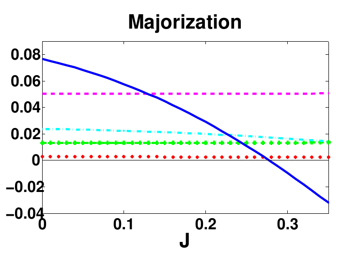

In summary, we have shown that if the majorisation relation () is satisfied, then the model works like an engine (PWC). However, it is important to note that the PWC can hold even if the majorisation relation is not satisfied, as depicted in Fig. 3. For the coupled model, it implies that net work may be obtained () for . Given that along with the conditions (14) and (29), all majorisation inequalities hold and thus yield sufficient criteria for PWC in the case of system. On the other hand, for the single spin, we obtained sufficient and necessary conditions from majorisation. Finally, based on induction, we can infer sufficient criteria for the general case of system, which are the conditions: , and , within which PWC holds for the system. The details are mentioned in Appendix B.
VI Analysis of local work
Now, each spin constituting the bipartite coupled system is governed by a local Hamiltonian which also depends on the parameter , and so undergoes a cyclic evolution. Thus, it is of intact to examine the local performance of each spin in the quantum Otto cycle. The local state of each spin is obtained from its reduced density matrix. Thus, upon summing over the degrees of freedom of spin-1, the reduced density matrix for spin-1/2, in Stage-1, is defined as: , which may be written in diagonal form, as: , where is the occupation probability of the excited state, given by
| (30) |
and . The work performed by spin-1/2 is evaluated to be: . For convenience, we express this work in the form:
| (31) |
where has been defined in Eq. (19), and
| (32) |
Similarly, the reduced density matrix for spin-1, , is written as: , where the occupation probabilities:
| (33) | ||||
| (34) | ||||
| (35) |
are ordered as: . Then, the local work by spin-1 is given by: , which can be rewritten in the form:
| (36) |
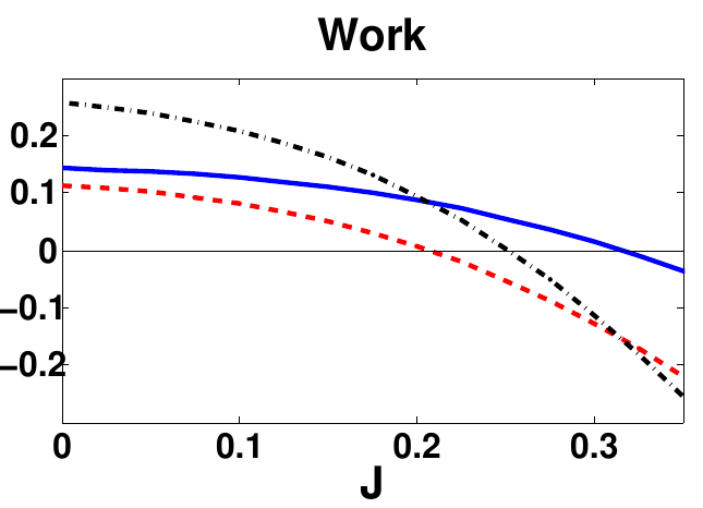
where we have used Eqs. (34) and (35) along with the definitions of and . Now, it is easily verified that the local work contributions, Eqs. (31) and (36), add up to yield the global work (Eq. (21)), i.e. . In Fig. 4, we compare the local and global work output. It is observed that the spin-1/2 work vanishes prior to the spin-1 work. This observation may be justified as follows.
As discussed earlier, for and , the majorisation relation () suggests the following set of sufficient conditions: and . From the majorisation inequalities, we have derived, in Section V.A, the condition or PWC for the global system. Furthermore, it can also be shown that sufficient conditions for PWC in spin-1/2 and spin-1 are respectively (see Appendix C.1),
| (37) |
| (38) |
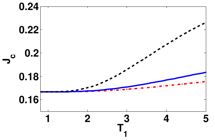
Now, let us analyze the behavior of local work in this range of values. From the analytic expressions as well as Fig. (5), we notice that at low temperatures. It implies that both local work and the global work are positive in . For higher temperatures, when , the critical values of follow: , which indicates that the work performed by spin-1/2 can be negative even when the global work and the local work due to spin-1 are positive. The same conclusion can be justified from the sign of . Thus, it can be proved that for (see Appendix C.2). Applied to Eq. (36), this result implies that the local work by spin-1 is always positive provided the global work is positive () for . Analogously, it can be inferred from Eq. (31) that for values of , the work performed by spin-1/2 can be negative even when the global work is positive.
Thus, we can summarize that in the range , both spin-1/2 and spin-1 yield positive work, and so the global work is positive. Beyond this range (), spin-1/2 may yield negative work even when the global work is positive. However, spin-1 yields positive work only if global work is positive. The local work analysis can be extended to the general case of coupled which is described in Appendix C.1.
VII Enhancement of Otto efficiency

The quantum feature of exchange coupling as a resource to enhance the Otto efficiency has been studied in earlier works. In Ref. Thomas and Johal 2011, an upper bound for Otto efficiency which is tighter than the Carnot limit was derived. In the following, we revisit the feature of efficiency enhancement and provide justification for the upper bound based on the majorisation approach.
The efficiency of the QOE, can be expressed using Eqs. (18) and (21) as:
| (39) |
where is the efficiency of uncoupled system which is the same regardless of the magnitudes of individual spin. We have seen that owing to consistency with the second law, the quantum Otto efficiency is bounded from above by the Carnot value, . However, heuristics can be applied to this system Johal and Mehta 2021 to obtain a tighter upper bound on the efficiency, which is given by:
| (40) |
Thus it can be seen that in the range , the above bound is lower than the Carnot value, and is saturated for , as shown in Fig. 6.
Now, we show how the majorisation relation reveals this upper bound for Otto efficiency. We have seen is positive in the range . The expression for suggests that in the presence of coupling (), the condition enhances the efficiency over the uncoupled model (). Now, combining with global majorisation condition (Eq. (27)), we can write:
| (41) |
implying that
which is satisfied in the range , indicating the efficiency enhancement region. The Otto efficiency is depicted in Fig. 6.
Now, consider the expression, . Adding the inequalities (22), (23) and (25), and upon rearranging terms, we obtain , or . Then, from Eq. (39), this implies that in the domain of the majorisation relation (), the efficiency has the upper bound given by . The proof can be extended to the general case of system, which is discussed in Appendix D.
VIII Conclusions
QOE is one of the most well studied models of a quantum heat engine. It is based on generalizations of the classical adiabatic and isochoric processes. Further, a spin-based working medium provides a convenient platform to investigate quantum features and their advantages for a QOE. Thus a QOE based on spin-1/2 particle is well known to have an efficiency, Kieu 2004. Also, is a necessary condition, given that and . The additional condition guarantees PWC, which can be seen from the expression for work extracted in a QOE:
| (42) |
We have shown that PWC for a QOE based on an arbitrary spin can be derived from the concept of majorisation between and , whereby the relation provides a necessary and sufficient condition for PWC. Further, we have expressed the work output in a QOE in terms of the relative entropies and . It is clarified in general that is necessary, but not a sufficient condition for PWC. Further, the total entropy generated in a quantum Otto cycle is given by the sum total of the two relative entropies.
Then, we have considered a spin-1/2 interacting with a spin- via 1-d Heisenberg exchange interaction with isotropic coupling strength . In this case, majorisation yield PWC, provided we impose and additionally restrict . The critical value provides a sufficient range for parameter such that the majorisation inqualities hold good. We have treated the case in detail and provided expressions for the case with a general value, in the Appendix. It is important to remark that in Ref. Johal and Mehta 2021, an extreme case scenario was used to infer the permissible range of as . Since, , so the range inferred in this paper extends the previous range of Ref. Johal and Mehta 2021.
Using the global majorisation inequalities, we have also investigated the local thermodynamics of spins. Thereby, it is possible to infer that spin-1/2 ceases to yield work at a certain value, while spin-1 continues to output work at larger values. The global work vanishes in between these two values, giving . Again, in previous works Thomas and Johal 2011; Johal and Mehta 2021, an enhancement of efficiency was reported for the coupled model and an upper bound for the Otto efficiency was inferred which is tighter than the Carnot value. In the present work, we have justified this bound using majorisation inequalities. All these results can be extended to a (1/2,) system.
In conclusion, our analysis shows that majorisation relation can usefully characterize the operational conditions for a quantum Otto engine based on spins as the working medium. The approach based on majorisation is able to highlight key qualitative features of even the local spin cycles. It will be interesting to extend the analysis to other interacting models Zhang 2008; Azimi et al. 2014; Yunger Halpern et al. 2019. Thus, majorisation is expected to serve as a key heuristic in inferring the thermodynamic features of complex working media in a quantum heat engine.
Acknowledgment
SS acknowledges financial support in the form of Senior Research Fellowship from the Council for Scientific and Industrial Research (CSIR) via Award No. 09/947(0250)/2020-EMR-I India.
Appendix A Work output in terms of relative entropy
We consider a quasi-static quantum Otto engine (QOE) in the presence of two heat reservoirs at temperatures and , as described in the main text.
The heat exchange at hot and cold reservoirs are given respectively as:
| (43) |
The work output in one quantum Otto cycle is given by:
| (44) |
where
| (45) |
are the canonical occupation probabilities for the system while it is in equilibrium with hot and cold reservoirs, respectively. and are the corresponding canonical partition sums. We have set Boltzmann’s constant equal to unity. The above relations can be inverted as
| (46) |
and substituted in Eq. (43), to obtain
| (47) |
We have applied the normalization conditions , added and subtracted suitable terms to write the above as follows.
| (48) |
Similarly,
| (49) |
Upon rearranging the terms on the rhs of the above equation, we can write
| (51) |
where and is Shannon entropy of the system in contact with hot and cold reservoirs respectively, while and are the alternate forms of Kullback-Leibler divergence (relative entropy) between the distributions and .
Appendix B PWC for the coupled system
The special case of coupled system has been described in the main text. Here, we considered the more general case of two coupled spins, denoted as system, whose energy spectrum is shown in Fig. 1. The total number of energy levels is .
⋮
⋮
⋮
⋮
Fig. 1: Energy eigenvalue spectrum for coupled system (see Johal and Mehta 2021).
The heat exchanged at the hot reservoir can be written as
| (52) |
where
| (53) | ||||
| (54) |
Similarly, the heat exchanged at the cold reservoir is given by . So, the net work performed in one cycle is given as:
| (55) |
Now, we prove the positive work condition (PWC) i.e. for the case . We assume the majorisation relation (), which implies the validity of the following set of inequalities:
| (56) | ||||
| (57) | ||||
| (58) | ||||
| (59) | ||||
In all, there are inequalities in the above, which is an odd number since is even. Now, starting from the top, adding up all the alternate inequalities (Eqs. (56), (58), and so on up to (59)), and upon rearranging, we conclude that . Again, the special case of has been discussed in detail in the main text.
This proves that the majorisation relation () implies the PWC for the quantum Otto cycle based on the coupled system.
From the normalization condition on probabilities and Eq. (59), we get
Appendix C Local thermodynamics of individual spins
C.1 Local work analysis for (1/2,s) system
After showing that the majorisation relation for the coupled system implies PWC, we proceed to analyze the thermodynamic behavior of individual spins. Our interest is to see up to what extent the global majorisation relations determine the operation of each spin. First, we note that the probability distribution for the reduced state of spin- is given by
| (64) | ||||
| (65) |
Here, is the ground state probability for spin-1/2. Similarly, the probability distribution for the reduced state of spin- is given by:
| (66) | ||||
| (67) | ||||
| (68) |
where . Clearly, these expressions reduce to those given in the main text for the case .
Then, the work performed by spin-1/2 can be calculated to be:
| (69) |
and work by spin- is given as:
| (70) |
where is given by Eq. (53) and
It can be seen that the sum total of the local contributions to work add up to yield the global work, , as given in Eq. (55).
(i) PWC for spin-1/2
Given , PWC for spin-1/2 requires,
| (73) |
Combining global majorisation condition Eq. (60) and Eq. (73), we obtained sufficient condition for PWC on coupling constant (),
| (74) |
(ii) PWC for spin-s
Given , PWC for spin-s requires,
| (75) |
C.2 Local work analysis for system
In this section, we derive PWC for individual spins, assuming global majorisation relation. Thus we have following set of conditions (),
| (77) | ||||
| (78) | ||||
| (79) | ||||
| (80) | ||||
| (81) |
Due to normalization of each probability distribution, Eq. (81) implies:
| (82) |
PWC for spin-1/2:
From Eq. (69), the PWC for spin-1/2 requires:
| (83) |
On using Eq. (53) and Eq. (C.1) for s=1, we can write
| (84) |
Combining Eq. () and Eq. (84), we get
| (85) |
which implies the following:
| (86) | ||||
that can be rearranged as follows:
| (87) |
Now, for , the first, second and fourth terms in square brackets above are positive. Positivity of the third and fifth terms together implies,
| (88) |
Which bound value as:
| (89) |
This implies that is a sufficient condition for PWC in case of spin-1/2.
PWC for spin-1:
From Eq. (70), PWC for spin-1 requires:
| (90) |
On using Eqs. (53)and (C.1) for s=1, we can write
| (91) |
Combining Eqs. () and (91), we get
| (92) |
On rearranging, we get
| (93) |
Now, for , the first, second, and fourth terms in square brackets above are positive. Positivity of the third and fifth terms gives,
| (94) |
with the range given by:
| (95) |
This implies that is a sufficient condition for PWC in case of the spin-1 subsystem.
In the following, we give explicit proof of for in case system. For this system,
| (96) |
Proof: Let us suppose , so that
Plugging in the explicit forms of the canonical probabilities in the above, we obtain
| (97) |
Simplify further, we get
| (98) |
The conditions, , and , favor the above inequality. However, the following terms have ambiguous relation:
However, if we consider the best case scenario, such that these terms also favor the inequality , then we must have
which implies that . Thus, for , we have .
The extension of the above proof for the general case (Eq.(C.1)) gives .
implies that the work performed by higher spin will always be positive when the global work is positive (), and the work performed by spin-1/2 can be negative even when the global work is positive.
Appendix D An upper bound for Otto efficiency
The efficiency of QOE is defined as: , which can be written as
| (99) |
or
| (100) |
where is the efficiency of the uncoupled system (). and are defined Eqs. (53) and (54). We have seen that for . Therefore, gives the region where efficiency can be enhanced over that of the uncoupled system. From Eq. (54), we note that the expression for involves only the levels which also depend on parameter . It is these levels that contribute to a decrease in the heat which is not converted into work due to the fixed nature of parameter . If the net flow of heat through these levels can be from cold to hot, then the efficiency may be enhanced Thomas and Johal 2011; de Oliveira and Jonathan 2021.
From majorisation inequalities and using the expressions for and given above, we can show
| (101) |
The special case of the (1/2,1) system has been described in the paper. Based on this, we can infer an upper bound for the Otto efficiency as
| (102) |
The above bound provides a useful upper bound as long as it stays lower than the Carnot value, i.e. for .
References
- Vinjanampathy and Anders (2016) S. Vinjanampathy and J. Anders, Quantum thermodynamics, Contemporary Physics 57, 545 (2016).
- Kosloff (2013) R. Kosloff, Quantum thermodynamics: A dynamical viewpoint, Entropy 15, 2100 (2013).
- Millen and Xuereb (2016) J. Millen and A. Xuereb, Perspective on quantum thermodynamics, New Journal of Physics 18, 011002 (2016).
- Quan et al. (2007) H. Quan, Y.-x. Liu, C. Sun, and F. Nori, Quantum thermodynamic cycles and quantum heat engines, Phys. Rev. E 76, 031105 (2007).
- Scovil and Schulz-DuBois (1959) H. E. D. Scovil and E. O. Schulz-DuBois, Three-level masers as heat engines, Phys. Rev. Lett. 2, 262 (1959).
- Alicki (2014) R. Alicki, Quantum thermodynamics: An example of two-level quantum machine, Open Systems & Information Dynamics 21, 1440002 (2014).
- Rivas (2020) Á. Rivas, Strong coupling thermodynamics of open quantum systems, Phys. Rev. Lett. 124, 160601 (2020).
- Goold et al. (2016) J. Goold, M. Huber, A. Riera, L. Del Rio, and P. Skrzypczyk, The role of quantum information in thermodynamics—a topical rev., Journal of Physics A: Mathematical and Theoretical 49, 143001 (2016).
- Jiao et al. (2021) G. Jiao, S. Zhu, J. He, Y. Ma, and J. Wang, Fluctuations in irreversible quantum Otto engines, Phys. Rev. E 103, 032130 (2021).
- Albash et al. (2012) T. Albash, S. Boixo, D. A. Lidar, and P. Zanardi, Quantum adiabatic markovian master equations, New Journal of Physics 14, 123016 (2012).
- Chitambar and Gour (2019) E. Chitambar and G. Gour, Quantum resource theories, Rev. Mod. Phys. 91, 025001 (2019).
- Esposito et al. (2010) M. Esposito, K. Lindenberg, and C. V. den Broeck, Entropy production as correlation between system and reservoir, New Journal of Physics 12, 013013 (2010).
- Maruyama et al. (2009) K. Maruyama, F. Nori, and V. Vedral, Colloquium: The physics of maxwell’s demon and information, Rev. Mod. Phys. 81, 1 (2009).
- Parrondo et al. (2015) J. M. Parrondo, J. Horowitz, and T. Sagawa, Thermodynamics of information, Nature Physics 11, 131 (2015).
- Popescu et al. (2006) S. Popescu, A. Short, and A. Winter, Entanglement and the foundations of statistical mechanics, Nature Physics 2, 754 (2006).
- Alicki (1979) R. Alicki, The quantum open system as a model of the heat engine, Journal of Physics A 12 (1979).
- Allahverdyan et al. (2008) A. E. Allahverdyan, R. S. Johal, and G. Mahler, Work extremum principle: Structure and function of quantum heat engines, Phys. Rev. E 77, 041118 (2008).
- Zhang et al. (2022) K. Zhang, X. Wang, Q. Zeng, and J. Wang, Conditional entropy production and quantum fluctuation theorem of dissipative information: Theory and experiments, PRX Quantum 3, 030315 (2022).
- Landi and Paternostro (2021) G. T. Landi and M. Paternostro, Irreversible entropy production: From classical to quantum, Rev. Mod. Phys. 93, 035008 (2021).
- Esposito et al. (2015) M. Esposito, M. A. Ochoa, and M. Galperin, Quantum thermodynamics: A nonequilibrium green’s function approach, Phys. Rev. Lett. 114, 080602 (2015).
- Singh et al. (2020) V. Singh, T. Pandit, and R. S. Johal, Optimal performance of a three-level quantum refrigerator, Phys. Rev. E 101, 062121 (2020).
- Maffei et al. (2021) M. Maffei, P. A. Camati, and A. Auffèves, Probing nonclassical light fields with energetic witnesses in waveguide quantum electrodynamics, Phys. Rev. Research 3, L032073 (2021).
- Rubio et al. (2021) J. Rubio, J. Anders, and L. A. Correa, Global quantum thermometry, Phys. Rev. Lett. 127, 190402 (2021).
- Alves and Landi (2022) G. O. Alves and G. T. Landi, Bayesian estimation for collisional thermometry, Phys. Rev. A 105, 012212 (2022).
- Camati et al. (2019) P. A. Camati, J. F. G. Santos, and R. M. Serra, Coherence effects in the performance of the quantum Otto heat engine, Phys. Rev. A 99, 062103 (2019).
- Alet et al. (2021) F. Alet, M. Hanada, A. Jevicki, and C. Peng, Entanglement and confinement in coupled quantum systems, Journal of High Energy Physics 2021, 34 (2021).
- Zhang et al. (2007) T. Zhang, W.-T. Liu, P.-X. Chen, and C.-Z. Li, Four-level entangled quantum heat engines, Phys. Rev. A 75, 062102 (2007).
- Albayrak (2013) E. Albayrak, The entangled quantum heat engine in the various heisenberg models for a two-qubit system, International Journal of Quantum Information 11, 1350021 (2013).
- de la Cruz and Martin-Delgado (2014) J. M. D. de la Cruz and M. A. Martin-Delgado, Quantum-information engines with many-body states attaining optimal extractable work with quantum control, Physical Review A 89, 10.1103/physreva.89.032327 (2014).
- Campisi et al. (2015) M. Campisi, J. Pekola, and R. Fazio, Nonequilibrium fluctuations in quantum heat engines: Theory, example, and possible solid state experiments, New Journal of Physics 17 (2015).
- Myers and Deffner (2020) N. M. Myers and S. Deffner, Bosons outperform fermions: The thermodynamic advantage of symmetry, Phys. Rev. E 101, 012110 (2020).
- Watanabe et al. (2020) G. Watanabe, B. P. Venkatesh, P. Talkner, M.-J. Hwang, and A. del Campo, Quantum statistical enhancement of the collective performance of multiple bosonic engines, Phys. Rev. Lett. 124, 210603 (2020).
- Wu et al. (2014) F. Wu, J. He, Y. Ma, and J. Wang, Efficiency at maximum power of a quantum Otto cycle within finite-time or irreversible thermodynamics, Phys. Rev. E 90, 062134 (2014).
- Peña et al. (2020) F. J. Peña, D. Zambrano, O. Negrete, G. De Chiara, P. A. Orellana, and P. Vargas, Quasistatic and quantum-adiabatic Otto engine for a two-dimensional material: The case of a graphene quantum dot, Phys. Rev. E 101, 012116 (2020).
- Das and Mukherjee (2020) A. Das and V. Mukherjee, Quantum-enhanced finite-time Otto cycle, Phys. Rev. Research 2, 033083 (2020).
- Chand et al. (2021) S. Chand, S. Dasgupta, and A. Biswas, Finite-time performance of a single-ion quantum Otto engine, Phys. Rev. E 103, 032144 (2021).
- Lee et al. (2020) S. Lee, M. Ha, J.-M. Park, and H. Jeong, Finite-time quantum Otto engine: Surpassing the quasistatic efficiency due to friction, Phys. Rev. E 101, 022127 (2020).
- Türkpençe and Altintas (2019) D. Türkpençe and F. Altintas, Coupled quantum Otto heat engine and refrigerator with inner friction, Quantum Information Processing 18, 255 (2019).
- Thomas and Johal (2014) G. Thomas and R. S. Johal, Friction due to inhomogeneous driving of coupled spins in a quantum heat engine, The European Phys. Journal B 87, 166 (2014).
- Geva and Kosloff (1992) E. Geva and R. Kosloff, A quantum-mechanical heat engine operating in finite time. a model consisting of spin-1/2 systems as the working fluid, The Journal of Chemical Physics 96, 3054 (1992).
- Feldmann and Kosloff (2000) T. Feldmann and R. Kosloff, Performance of discrete heat engines and heat pumps in finite time, Phys. Rev. E 61, 4774 (2000).
- Çakmak et al. (2017) S. Çakmak, F. Altintas, A. Gençten, and Ö. E. Müstecaplıoğlu, Irreversible work and internal friction in a quantum Otto cycle of a single arbitrary spin, The European Phys. Journal D 71, 75 (2017).
- Shastri and Venkatesh (2022) R. Shastri and B. P. Venkatesh, Optimization of asymmetric quantum otto engine cycles, Phys. Rev. E 106, 024123 (2022).
- Solfanelli et al. (2020) A. Solfanelli, M. Falsetti, and M. Campisi, Nonadiabatic single-qubit quantum otto engine, Phys. Rev. B 101, 054513 (2020).
- Papadatos (2021) N. Papadatos, The quantum otto heat engine with a relativistically moving thermal bath, International Journal of Theoretical Physics 60, 4210 (2021).
- Das and Ghosh (2019) A. Das and S. Ghosh, Measurement based quantum heat engine with coupled working medium, Entropy 21, 10.3390/e21111131 (2019).
- Peña et al. (2020) F. J. Peña, O. Negrete, N. Cortés, and P. Vargas, Otto engine: Classical and quantum approach, Entropy 22, 10.3390/e22070755 (2020).
- Lin and Chen (2003) B. Lin and J. Chen, Performance analysis of an irreversible quantum heat engine working with harmonic oscillators, Phys. Rev. E 67, 046105 (2003).
- Rezek and Kosloff (2006) Y. Rezek and R. Kosloff, Irreversible performance of a quantum harmonic heat engine, New Journal of Physics 8, 83 (2006).
- Zhang (2008) G.-F. Zhang, Entangled quantum heat engines based on two two-spin systems with Zyaloshinski-Moriya anisotropic antisymmetric interaction, The European Phys. Journal D 49, 123 (2008).
- Hübner et al. (2014) W. Hübner, G. Lefkidis, C. Dong, D. Chaudhuri, L. Chotorlishvili, and J. Berakdar, Spin-dependent Otto quantum heat engine based on a molecular substance, Phys. Rev. B 90, 024401 (2014).
- Azimi et al. (2014) M. Azimi, L. Chotorlishvili, S. K. Mishra, T. Vekua, W. Hübner, and J. Berakdar, Quantum Otto heat engine based on a multiferroic chain working substance, New Journal of Physics 16, 063018 (2014).
- Insinga et al. (2016) A. Insinga, B. Andresen, and P. Salamon, Thermodynamical analysis of a quantum heat engine based on harmonic oscillators, Phys. Rev. E 94, 012119 (2016).
- Mehta and Johal (2017) V. Mehta and R. S. Johal, Quantum Otto engine with exchange coupling in the presence of level degeneracy, Phys. Rev. E 96, 032110 (2017).
- Peterson et al. (2019) J. P. S. Peterson, T. B. Batalhão, M. Herrera, A. M. Souza, R. S. Sarthour, I. S. Oliveira, and R. M. Serra, Experimental characterization of a spin quantum heat engine, Phys. Rev. Lett. 123, 240601 (2019).
- Myers et al. (2022) N. M. Myers, O. Abah, and S. Deffner, Quantum thermodynamic devices: From theoretical proposals to experimental reality, AVS Quantum Science 4, 027101 (2022), https://doi.org/10.1116/5.0083192 .
- Marshall et al. (2011) A. W. Marshall, I. Olkin, and B. C. Arnold, Inequalities: Theory of majorisation and its applications (Springer Series in Statistics, Springer, New York, 2011).
- Sagawa (2020) T. Sagawa, Entropy, divergence, and majorisation in classical and quantum thermodynamics (SpringerBriefs in Mathematical Physics, Springer Singapore, 2020).
- Bhatia (1996) R. Bhatia, Matrix analysis (Springer New York, NY, 1996).
- Buscemi and Gour (2017) F. Buscemi and G. Gour, Quantum relative lorenz curves, Phys. Rev. A 95, 012110 (2017).
- Joe (1990) H. Joe, Majorisation and divergence, Journal of Mathematical Analysis and Applications 148, 287 (1990).
- Shiraishi (2020) N. Shiraishi, Two constructive proofs on d-majorisation and thermo-majorisation, Journal of Physics A: Mathematical and Theoretical 53, 425301 (2020).
- Egloff et al. (2015) D. Egloff, O. C. O. Dahlsten, R. Renner, and V. Vedral, A measure of majorisation emerging from single-shot statistical mechanics, New Journal of Physics 17, 073001 (2015).
- Nielsen and Vidal (2001) M. A. Nielsen and G. Vidal, Majorisation and the interconversion of bipartite states, Quantum Info. Comput. 1, 76–93 (2001).
- Rethinasamy and Wilde (2020) S. Rethinasamy and M. M. Wilde, Relative entropy and catalytic relative majorisation, Phys. Rev. Research 2, 033455 (2020).
- Renes (2016) J. M. Renes, Relative submajorisation and its use in quantum resource theories, Journal of Mathematical Physics 57, 122202 (2016).
- Ruch et al. (1980) E. Ruch, R. Schranner, and T. H. Seligman, Generalization of a theorem by hardy, littlewood, and pólya, Journal of Mathematical Analysis and Applications 76, 222–229 (1980).
- Nielsen (1999) M. A. Nielsen, Conditions for a class of entanglement transformations, Phys. Rev. Lett. 83, 436 (1999).
- Du et al. (2015) S. Du, Z. Bai, and Y. Guo, Conditions for coherence transformations under incoherent operations, Phys. Rev. A 91, 052120 (2015).
- Jonathan and Plenio (1999) D. Jonathan and M. B. Plenio, Entanglement-assisted local manipulation of pure quantum states, Phys. Rev. Lett. 83, 3566 (1999).
- Horodecki et al. (2003) M. Horodecki, P. Horodecki, and J. Oppenheim, Reversible transformations from pure to mixed states and the unique measure of information, Phys. Rev. A 67, 062104 (2003).
- Gour et al. (2018) G. Gour, D. Jennings, F. Buscemi, R. Duan, and I. Marvian, Quantum majorisation and a complete set of entropic conditions for quantum thermodynamics, Nature Communications 9, 10.1038/s41467-018-06261-7 (2018).
- Brandão et al. (2015) F. Brandão, M. Horodecki, N. Ng, J. Oppenheim, and S. Wehner, The second laws of quantum thermodynamics, Proceedings of the National Academy of Sciences 112, 3275–3279 (2015).
- Horodecki and Oppenheim (2013) M. Horodecki and J. Oppenheim, Fundamental limitations for quantum and nanoscale thermodynamics, Nature Communications 4, 10.1038/ncomms3059 (2013).
- Zemansky (1968) M. W. Zemansky, Heat and thermodynamics; an intermediate textbook (McGraw-Hill New York, 1968).
- Born and Fock (1928) M. Born and V. Fock, Beweis des Adiabatensatzes, Zeitschrift fur Physik 51, 165 (1928).
- Kullback and Leibler (1951) S. Kullback and R. A. Leibler, On Information and Sufficiency, The Annals of Mathematical Statistics 22, 79 – 86 (1951).
- Kieu (2004) T. D. Kieu, The second law, Maxwell’s demon, and work derivable from quantum heat engines, Phys. Rev. Lett. 93, 140403 (2004).
- Johal and Mehta (2021) R. S. Johal and V. Mehta, Quantum heat engines with complex working media, complete Otto cycles and heuristics, Entropy 23, 1149 (2021).
- Thomas and Johal (2011) G. Thomas and R. S. Johal, Coupled quantum Otto cycle, Phys. Rev. E 83, 031135 (2011).
- Altintas and Müstecaplıoğlu (2015) F. Altintas and O. E. Müstecaplıoğlu, General formalism of local thermodynamics with an example: Quantum Otto engine with a spin- coupled to an arbitrary spin, Phys. Rev. E 92, 022142 (2015).
- Yunger Halpern et al. (2019) N. Yunger Halpern, C. D. White, S. Gopalakrishnan, and G. Refael, Quantum engine based on many-body localization, Phys. Rev. B 99, 024203 (2019).
- de Oliveira and Jonathan (2021) T. R. de Oliveira and D. Jonathan, Efficiency gain and bidirectional operation of quantum engines with decoupled internal levels, Phys. Rev. E 104, 044133 (2021).