Physical significance of generalized boundary conditions:
an Unruh-DeWitt detector viewpoint on Journal: …
Abstract
On , we construct the two-point correlation functions for the ground and thermal states of a real Klein-Gordon field admitting generalized -boundary conditions. We follow the prescription recently outlined in [1] for two different choices of secondary solutions. For each of them, we obtain a family of admissible boundary conditions parametrized by . We study how they affect the response of a static Unruh-DeWitt detector. The latter not only perceives variations of , but also distinguishes between the two families of secondary solutions in a qualitatively different, and rather bizarre, fashion. Our results highlight once more the existence of a freedom in choosing boundary conditions at a timelike boundary which is greater than expected and with a notable associated physical significance.
Keywords:
Generalized Robin boundary conditions , Unruh-DeWitt detector , Klein-Gordon field ,1 Introduction
Since the introduction of Unruh-DeWitt particle detectors in quantum field theory [2, 3], they have been employed to probe a plethora of features of quantum fields and of spacetimes, stretching from picking out properties of quantum states [4] to identifying topological aspects of underlying backgrounds [5]. On a globally-hyperbolic spacetime with a timelike boundary, they are particularly sensible to the choice of an underlying boundary condition for the matter fields: phenomena such as the divergence of physical observables [6, 7] and the anti-Hawking effect [8, 9] depend crucially on the boundary condition set. This is consonant with the fact that different boundary conditions are associated to different quantum states, to different dynamics, to different physics [10].
In this arena we have recently shown that within free, scalar quantum field theories on static, curved spacetimes with a timelike boundary one may take into account generalized -Robin boundary conditions in the construction of physically meaningful states [1]. These arise whenever the underlying dynamics can be reduced thanks to the background isometries to a second order differential equation on the half line and they are characterized by two data: a fixed parameter and a so-called secondary solution . For each admissible pair , one can construct a two-point function both for the ground state and also for arbitrary thermal states. All these correlation functions are physically sensible since, per construction, they enjoy the local Hadamard property, see [11]. In [1], we have discussed the example of a wave propagating on the two-dimensional half-Minkowski spacetime showing that an Unruh-DeWitt detector can discern not only the value of , but also the choice of secondary solution . Here, we elaborate on this idea and we provide, in full detail, a full-fledged example that demonstrates how the hidden freedom in the mode expansion of the scalar field, which is associated to the choice of , influences the rate of transition of an Unruh-DeWitt particle detector.
In this work, we consider a real, free, scalar field with mass on spacetime. This background approximates the near horizon geometry of an extremal black hole with unit charge and it is known as the Bertotti-Robinson solution of Einstein-Maxwell equations, see e.g. [12] but also [13, 14]. For and , its line-element can be written as
| (1) |
where is the standard line-element on the unit -sphere. Observe that the manifold possesses a timelike conformal boundary at . On top of we consider a real scalar field whose dynamics is ruled by the Klein-Gordon equation
| (2) |
where is the D’Alembert wave operator built out of Equation (1), while is the mass parameter.
In Section 2, we recollect the main ingredients necessary to construct the two-point functions for ground and thermal states for . The procedure follows the prescription outlined in [1] and it generalizes the results obtained in [15] by considering two different families of generalized -boundary conditions at the conformal boundary, dubbed with . The analysis for coincides with that of [15], while for it yields novel two-point functions. Nonetheless, since also in this case the overall analysis is structurally identical to that for , we do not dwell into many details and we limit ourselves to sketching the main steps of the construction.
Subsequently, in Section 3 we obtain an explicit expression for the transition rate of a static Unruh-DeWitt detector interacting either with the ground or with a thermal state of a Klein-Gordon field. We scrutinize the response of the detector to grasp if and how it is affected by the choice of boundary condition. In particular, we focus on the consequences of the freedom in selecting a secondary solution in the construction of Section 2. In Section 4, we summarize the main results of this work.
2 Dynamics and Boundary Conditions
Working with the coordinates of Equation (1), a real Klein-Gordon field that solves Equation (2) can be decomposed as
where are the spherical harmonics on the -dimensional unit sphere. Setting , the function solves the radial equation
| (3) |
2.1 The radial equation
In the following we assume that and we introduce the auxiliary quantities
| (4) |
subject to the constraint . Equation (3) is a Sturm-Liouville problem with eigenvalue , which admits a basis of solutions written in terms of Bessel functions of first and second kind:
| (5a) | ||||
| (5b) | ||||
Following [16], it is convenient to work on the Hilbert space and allow to take a priori any complex value. Hence, according to Weyl’s endpoint classification is a limit point, see also [15] for a succinct summary of the nomenclature. As a matter of fact, assuming that , the most general solution of Equation (3) lying in , can be written in terms of Hankel functions of first and second kind:
On the other hand, it turns out that is a limit circle point if , since both , , as one can infer from the following asymptotic expansion close to the origin:
Observe that
| (6) |
Still following the theory of Sturm-Liouville, this entails that only the mode calls for a boundary condition at , provided that the mass lies in the range individuated in Equation (6). When , no boundary condition needs to be imposed at both ends and since this case is not of interest in this work, we shall not consider it further.
2.2 Generalized -boundary conditions
At the limit circle endpoint, , we impose generalized -boundary conditions as introduced in [1]. These identify self-adjoint extensions of the radial operator in and they are fully characterized in terms of a parameter , of the principal solution, , and of a secondary solution, , which we introduce in the following. The principal solution at reads
This is unambiguously identified by the condition that, for any solution of Equation (3) such that , , then . On the contrary choosing a secondary solution at , linearly independent from , is fully arbitrary. In the following we consider two possible choices , :
| (7a) | ||||
| (7b) | ||||
In terms of the basis given in Equation (5), they can be written as
For and , it follows that the solution
satisfies
| (8) |
where denotes the Wronskian . If Equation (8) holds true, we say that satisfies a -boundary condition at .
2.3 The radial Green function
In the next step in our analysis we construct the Green function of the radial equation. To this end, it is convenient to rewrite the solution at infinity as a linear combination of and :
A direct computation yields
where , and . Since , it descends
Therefore, following [17], if is the operator as per Equation (3), the radial Green function, implicitly defined by
reads
| (9) |
where is a shortcut notation for the integral kernel .
2.4 Symmetries of the radial Green function
2.5 Bound States
When choosing a boundary condition in Equation (8), we consider as admissible the values of for which there does not exist such that diverges. In other words, at a physical level, we rule out those boundary conditions for which has bound state frequencies . The case for is analogous to the computation on Minkowski spacetime in spherical coordinates as in [18, Pg.66], while the case for has been studied in detail in [15, Pg.10]. Here, we report the final result: neither nor possesses bound state frequencies for . Henceforth we restrict our attention to this interval. Observe that corresponds to the usual Dirichlet boundary condition. It is tempting to claim that, if , we are instead considering a Neumann boundary condition. This is indeed an admissible nomenclature, but the reader should keep in mind that the solution at of the radial equation depends only on the choice of the secondary solution, contrary to the case in which only plays a rôle. Hence there is no universal way to select a Neumann boundary condition, inasmuch as there does not exist a unique criterion to single out a secondary solution for Equation (3).
2.6 The resolution of the identity
In order to construct the two-point correlation function of the Klein-Gordon field with arbitrary -boundary condition, a last necessary ingredient is the so-called resolution of the identity for the radial equation. Following [17, Ch.7], this reads
| (12) |
where the contours differ if and they are illustrated in [1, Fig.1], while the integrand has been computed in [18]. Since its explicit form is not of relevance in this work, we shall not report it, although, for later convenience, we highlight that, whenever we restrict the attention to real, positive frequencies ,
where
2.7 Two-point correlation functions
In the preceding analysis we have individuated all the ingredients necessary to construct the two-point correlation function both of a ground and of a thermal state for a real Klein-Gordon field whose mass is such that one can endow it with physically admissible boundary conditions, i.e., . As in the previous sections, we shall not dwell into a detailed construction which has been already outlined in [18], but we limit ourselves to recalling the final result
| (13) |
where
| (14) |
For finite , Equation (13) together with Equation (14) characterize a thermal state at temperature . In the limit , we obtain instead the two-point correlation function of the ground state:
| (15) |
In the next section we shall use this class of two-point correlation functions to show that the choice of different secondary solutions associated to Equation (3) is not a mere mathematical exercise, but it bears strong physical consequences.
3 The transition rate
In this section we consider an Unruh-deWitt detector, namely a spatially localized two-level system that interacts with the underlying scalar field via a monopole type interaction. Here we are interested in computing and analyzing the transition rate when the detector follows static trajectories on . The detector can be initially either in the ground-state or in the excited state , see [2, 3]. This information is codified in the sign of its energy gap: corresponds to excitations, corresponds to de-excitations.
We let the detector interact for an infinite proper time with the Klein-Gordon field, whose initial state is either the ground state or a thermal state at inverse-temperature with -boundary conditions, see Equation (13). In addition, we parametrize the trajectory at fixed spatial coordinates by its proper time . In this setting, letting , the transition rate reads [19, 20]
| (16) |
Using the two-point functions as per Equation (14), as well as the addition formula between spherical harmonics, Equation (16) yields
where, being the Heaviside step function,
| (17) |
Observe that the variable must be evaluated at , but, for simplicity, we shall not indicate it explicitly in the following.
Recalling that only the term calls for a boundary condition, let us decompose the transition rate as
The component
| (18) |
corresponds to the contribution, while the remainder
| (19) |
is independent of both and .
There are two scenarios, i) and ii) as described in the following, where we can take the sum over giving an analytic expression for .
- i)
If , then and thus for . Consequently and, using the identity
we obtain
(20) - ii)
If , the secondary solution plays no rôle and it holds true that .
Note that if either i) or ii) holds true, then . Moreover, if both hold true, then using the expression obtained in item i) above, we get which is consistent with the fact that is conformal to Minkowski spacetime.
3.1 The contribution
In this section we focus on the term: . First, note that the secondary solutions and , as per Equation (7), are markedly different when is close to , that is for . Let us thus focus in this section on this mass range. We shall show that, for and , the detector behaves in a qualitatively different way for the various choices of secondary solution. We can verify it analytically and visualize it numerically, as shown next. As a matter of fact expanding as yields
| (21a) | ||||
| (21b) | ||||
The consequences of Equation (21) are two-fold:
- 1)
at zeroth order, the zeros of are those of and they do not depend on , while those do;
- 2)
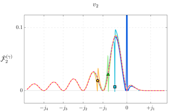
These features are manifest in Figure 1 which is displayed at the end of the paper for layout purposes. It contains line and contour plots of and of , respectively in the left and right columns. This numerical evaluation was performed using the software Mathematica and it is presented in a notebook available online [21]. For this analysis, we considered a field at inverse-temperature and of mass , which corresponds to . Consistently with the asymptotic expansion in Equation (21), Figure 1 displays the following notable features:
- 1.
The dashed, vertical white lines of subfigures (e) and (f) in Figure 1 correspond to the zeros of . These lines align with the zeros of for all as shown in subfigure (f), but this is not the case for , as shown in subfigure (e). Accordingly, we refer to this difference in behavior between and as a zeroth-order high-mass effect.
- 2.
The dashed, peaked, red line of subfigure (f) of Figure 1 codifies the identity . The restriction of this curve to subfigure (b) is given by the three highlighted points: the circle, the triangle and the square. We can see that these points indicate a first-order high-mass effect manifest only for , and that brings about an extra zero for that depends on the choice of .
 |
 |
 |
| (a) | (b) | |
 |
 |
 |
| (c) | (d) | |
 |
 |
Zeros of |
| (e) | (f) |
3.2 The sum over
The sum over conceals the high-mass effect discussed in the previous section, see Figure 2 that shows the transition rate summed up to with the same parameters of Figure 1. Nonetheless we can still disambiguate between the choices of secondary solution for the radial equation if, instead of checking out its zeros, we focus on the behaviour of the transition rate at . Figure 2 corroborates this statement, but it does not clarify what is happening at such locus. Yet, we can analytically compute the limit of for vanishing energy gap, as we show in the following.


For , we have that regardless of the value of the field mass. Thus, using the following two identities
one can show that
Consequently, the behavior of at depends only on the contribution from the term: , defined in Equation (18).
For vanishing mass, , . Since
we obtain that, for ,
| (22) |
Observe that if then diverges for . For positive masses, and the results are summarized in Table 1.
| State | |||
|---|---|---|---|
All in all, the boundary condition chosen for the mode affects the behavior of the transition rate in its full form, both quantitatively and qualitatively. In fact, its limit at receives no contribution from the terms with , as shown above. Markedly, the transition rate of an Unruh-DeWitt detector interacting with a Klein-Gordon field at a finite temperature state, with , and admitting a generalized -boundary condition with explicitly discriminates between and in Equation (7), as highlighted in blue in Table 1.
4 Outlook
We have shown that choosing one among the generalized -boundary conditions is not a mere mathematical exercise, rather it has notable physical consequences. For definiteness we have considered a Klein-Gordon field on spacetime and we have constructed the two-point correlation function of the ground and thermal states for two families of boundary conditions, characterized by different choices of secondary solution, and , see Equation (7). We probed the underlying system with an Unruh-DeWitt detector and we showed that its transition rate differentiates between the two families of boundary conditions.
There are two notable facts that highlight the hidden freedom in the mode expansion of the Klein-Gordon field and connect our results to [1]. First, the boundary conditions with and are equivalent at the level of the radial differential equation, but cease to be such at the level of the whole Klein-Gordon equation. This is hinted by the map that relates the parameter in the two settings. It depends on the Fourier frequency associated to the time coordinate and, therefore, we can map a solution satisfying Equation (8) for , into one satisfying it for via
There is an explicit dependence of the Fourier parameter which in turn related to the underlying frequency. This entails that, while, at the level of radial equation, this is a mere algebraic relation, from a fully covariant viewpoint, this is no longer true as one can realize by an inverse Fourier transform. Finally, our work sets the ground for multiple future investigations that are worth mentioning:
- 1.
comparisons between the physical phenomena associated to different choices of secondary solution, possibly considering other observables such as the stress-energy tensor;
- 2.
proving the universality of the features highlighted in this paper by studying their occurrence in other globally hyperbolic spacetimes with a timelike boundary, such as for example global monopoles and cosmic strings;
- 3.
- 4.
a further investigation of the behaviour of the transition rate at particularly in connection with the notion of a structureless scalar source [25].
5 Acknowledgments
The work of L.C. is supported by a postdoctoral fellowship of the Department of Physics of the University of Pavia, while that of L.S. by a PhD fellowship of the University of Pavia.
References
- [1] L. d. Campos, C. Dappiaggi and L. Sinibaldi, [arXiv:2207.08662 [gr-qc]].
- [2] W. G. Unruh, Phys. Rev. D 14, 870 (1976)
- [3] B. S.DeWitt “Quantum gravity: the new synthesis,” General Relativity: An Einstein Centenary Survey, 680–745, Cambridge University Press, Cambridge, England, (1979)
- [4] K. K. Ng, C. Zhang, J. Louko and R. B. Mann, [arXiv:2109.13260 [gr-qc]].
- [5] K. K. Ng, R. B. Mann and E. Martin-Martinez, Phys. Rev. D 96, no.8, 085004 (2017) [arXiv:1706.08978 [quant-ph]].
- [6] L. de Souza Campos and J. P. M. Pitelli, Phys. Rev. D 104, no.8, 085020 (2021) [arXiv:2108.12236 [hep-th]].
- [7] S. Namasivayam and E. Winstanley, [arXiv:2209.01133 [hep-th]].
- [8] L. J. Henderson, R. A. Hennigar, R. B. Mann, A. R. H. Smith and J. Zhang, Phys. Lett. B 809, 135732 (2020) [arXiv:1911.02977 [gr-qc]].
- [9] L. De Souza Campos and C. Dappiaggi, Phys. Lett. B 816, 136198 (2021) [arXiv:2009.07201 [hep-th]].
- [10] A. Ishibashi and R. M. Wald, Class. Quant. Grav. 20, 3815-3826 (2003) [arXiv:gr-qc/0305012 [gr-qc]].
- [11] I. Khavkine and V. Moretti, “Algebraic QFT in Curved Spacetime and quasifree Hadamard states: an introduction”: Algebraic QFT in Curved Spacetime and quasifree Hadamard states: an introduction. Published in: Chapter 5, Advances in Algebraic Quantum Field Theory, R. Brunetti et al. (eds.), Springer, (2015) [arXiv:1412.5945 [math-ph]].
- [12] A. Conroy and P. Taylor, Phys. Rev. D 105, no.8, 085001 (2022) [arXiv:2109.04486 [gr-qc]].
- [13] B. Bertotti, Phys. Rev. 116, 1331 (1959).
- [14] I. Robinson, Bull. Acad. Pol. Sci. 7, 351 (1959).
- [15] C. Dappiaggi and H. R. C. Ferreira, Phys. Rev. D 94, no.12, 125016 (2016) [arXiv:1610.01049 [gr-qc]].
- [16] A. Zettl, Sturm-Liouville Theory, American Mathematical Society, (2005).
- [17] I. Stakgold and M.J. Holst, “Green’s functions and boundary value problems”, John Wiley & Sons, 99 (2011).
- [18] L. De Souza Campos, [arXiv:2203.09976 [gr-qc]].
- [19] C. J. Fewster, B. A. Juárez-Aubry and J. Louko, Class. Quant. Grav. 33, no.16, 165003 (2016) [arXiv:1605.01316 [gr-qc]].
- [20] J. Louko and A. Satz, Class. Quant. Grav. 25, 055012 (2008) [arXiv:0710.5671 [gr-qc]].
- [21] Mathematica notebook, [https://github.com/lissadesouzacampos/physical_significance_generalized_bcs].
- [22] W. G. Brenna, R. B. Mann and E. Martin-Martinez, Phys. Lett. B 757, 307-311 (2016) [arXiv:1504.02468 [quant-ph]].
- [23] M. P. G. Robbins and R. B. Mann, Phys. Rev. D 106, no.4, 045018 (2022) [arXiv:2107.01648 [gr-qc]].
- [24] L. de Souza Campos and C. Dappiaggi, Phys. Rev. D 103, no.2, 025021 (2021) [arXiv:2011.03812 [hep-th]].
- [25] G. Cozzella, S. A. Fulling, A. G. S. Landulfo and G. E. A. Matsas, Phys. Rev. D 102, no.10, 105016 (2020) [arXiv:2009.13246 [hep-th]].