Hierarchical Neyman-Pearson Classification for Prioritizing Severe Disease Categories in COVID-19 Patient DataThanks: Correspondence should be addressed to Y.X. Rachel Wang (rachel.wang@sydney.edu.au)
Abstract
COVID-19 has a spectrum of disease severity, ranging from asymptomatic to requiring hospitalization. Understanding the mechanisms driving disease severity is crucial for developing effective treatments and reducing mortality rates. One way to gain such understanding is using a multi-class classification framework, in which patients’ biological features are used to predict patients’ severity classes. In this severity classification problem, it is beneficial to prioritize the identification of more severe classes and control the “under-classification” errors, in which patients are misclassified into less severe categories. The Neyman-Pearson (NP) classification paradigm has been developed to prioritize the designated type of error. However, current NP procedures are either for binary classification or do not provide high probability controls on the prioritized errors in multi-class classification. Here, we propose a hierarchical NP (H-NP) framework and an umbrella algorithm that generally adapts to popular classification methods and controls the under-classification errors with high probability. On an integrated collection of single-cell RNA-seq (scRNA-seq) datasets for patients, we explore ways of featurization and demonstrate the efficacy of the H-NP algorithm in controlling the under-classification errors regardless of featurization. Beyond COVID-19 severity classification, the H-NP algorithm generally applies to multi-class classification problems, where classes have a priority order.
1 Introduction
The COVID-19 pandemic has infected over 767 million people and caused 6.94 million deaths (27 June 2023) (World Health Organization 2023), prompting collective efforts from statistics and other communities to address data-driven challenges. Many statistical works have modeled epidemic dynamics (Betensky and Feng 2020; Quick et al. 2021), forecasted the case growth rates and outbreak locations (Brooks et al. 2020; Tang et al. 2021; McDonald et al. 2021), and analyzed and predicted the mortality rates (James et al. 2021; Kramlinger et al. 2022). Classification problems, such as diagnosis (positive/negative) (Wu et al. 2020; Li et al. 2020; Zhang et al. 2021) and severity prediction (Yan et al. 2020; Sun et al. 2020; Zhao et al. 2020; Ortiz et al. 2022), have been tackled by machine learning approaches (e.g., logistic regression, support vector machine (SVM), random forest, boosting, and neural networks; see Alballa and Al-Turaiki 2021 for a review).
In the existing COVID-19 classification works, the commonly used data types are CT images, routine blood tests, and other clinical data including age, blood pressure and medical history (Meraihi et al. 2022). In comparison, multiomics data are harder to acquire but can provide better insights into the molecular features driving patient responses (Overmyer et al. 2021). Recently, the increasing availability of single-cell RNA-seq (scRNA-seq) data offers the opportunity to understand transcriptional responses to COVID-19 severity at the cellular level (Wilk et al. 2020; Stephenson et al. 2021; Ren et al. 2021).
More generally, genome-wide gene expression measurements have been routinely used in classification settings to characterize and distinguish disease subtypes, both in bulk-sample (Aibar et al. 2015) and, more recently, single-cell level (Arvaniti and Claassen 2017; Hu et al. 2019). While such genome-wide data can be costly, they provide a comprehensive view of the transcriptome and can unveil significant gene expression patterns for diseases with complex pathophysiology, where multiple genes and pathways are involved. Furthermore, as the patient-level measurements continue to grow in dimension and complexity (e.g., from a single bulk sample to thousands-to-millions of cells per patient), a supervised learning setting enables us to better establish the connection between patient-level features and their associated disease states, paving the way towards personalized treatment.
In this study, we focus on patient severity classification using an integrated collection of multi-patient scRNA-seq datasets. Based on the WHO guidelines (World Health Organization 2020), COVID-19 patients have at least three severity categories: healthy, mild/moderate, and severe. The classical classification paradigm aims at minimizing the overall classification error. However, prioritizing the identification of more severe patients may provide important insights into the biological mechanisms underlying disease progression and severity, and facilitate the discovery of potential biomarkers for clinical diagnosis and therapeutic intervention. Consequently, it is important to prioritize the control of “under-classification” errors, in which patients are misclassified into less severe categories.
Motivated by the gap in existing classification algorithms for severity classification (Section 1.1), we propose a hierarchical Neyman-Pearson (H-NP) classification framework that prioritizes the under-classification error control in the following sense. Suppose there are classes with class labels ordered in decreasing severity. For , the -th under-classification error is the probability of misclassifying an individual in class into any class with . We develop an H-NP umbrella algorithm that controls the -th under-classification error below a user-specified level with high probability while minimizing a weighted sum of the remaining classification errors. Similar in spirit to the NP umbrella algorithm for binary classification in Tong et al. 2018, the H-NP umbrella algorithm adapts to popular scoring-type multi-class classification methods (e.g., logistic regression, random forest, and SVM). To our knowledge, the algorithm is the first to achieve asymmetric error control with high probability in multi-class classification.
Another contribution of this study is the exploration of appropriate ways to featurize multi-patient scRNA-seq data. Following the workflow in Lin et al. 2022a, we integrate 20 publicly available scRNA-seq datasets to form a sample of 864 patients with three levels of severity. For each patient, scRNA-seq data were collected from peripheral blood mononuclear cells (PBMCs) and processed into a sparse expression matrix, which consists of tens of thousands of genes in rows and thousands of cells in columns. We propose four ways of extracting a feature vector from each of these matrices. Then we evaluate the performance of each featurization way in combination with multiple classification methods under both the classical and H-NP classification paradigms. We note that our H-NP umbrella algorithm is applicable to other featurizations of scRNA-seq data, other forms of patient data, and more general disease classification problems with a severity ordering.
Below we review the NP paradigm and featurization of multi-patient scRNA-seq data as the background of our work.
1.1 Neyman-Pearson paradigm and multi-class classification
Classical binary classification focuses on minimizing the overall classification error, i.e., a weighted sum of type I and II errors, where the weights are the marginal probabilities of the two classes. However, the class priorities are not reflected by the class weights in many applications, especially disease severity classification, where the severe class is the minor class and has a smaller weight (e.g., HIV (Meyer and Pauker 1987) and cancer (Dettling and Bühlmann 2003)). One class of methods that addresses this error asymmetry is cost-sensitive learning (Elkan 2001; Margineantu 2002), which assigns different costs to type I and type II errors. However, such weights may not be easy to choose in practice, especially in a multi-class setting; nor do these methods provide high probability controls on the prioritized errors. The NP classification paradigm (Cannon et al. 2002; Scott and Nowak 2005; Rigollet and Tong 2011) was developed as an alternative framework to enforce class priorities: it finds a classifier that controls the population type I error (the prioritized error, e.g., misclassifying diseased patients as healthy) under a user-specified level while minimizing the type II error (the error with less priority, e.g., misdiagnosing healthy people as sick). Practically, using an order statistics approach, Tong et al. 2018 proposed an NP umbrella algorithm that adapts all scoring-type classification methods (e.g., logistic regression) to the NP paradigm for classifier construction. The resulting classifier has the population type I error under with high probability. Besides disease severity classification, the NP classification paradigm has found diverse applications, including social media text classification (Xia et al. 2021) and crisis risk control (Feng et al. 2021). Nevertheless, the original NP paradigm is for binary classification only.
Although several works aimed to control prioritized errors in multi-class classification (Landgrebe and Duin 2005; Xiong et al. 2006; Tian and Feng 2021), they did not provide high probability control. That is, if they are applied to severe disease classification, there is a non-trivial chance that their under-classification errors exceed the desired levels.
1.2 ScRNA-seq data featurization
In multi-patient scRNA-seq data, every patient has a gene-by-cell expression matrix; genes are matched across patients, but cells are not. For learning tasks with patients as instances, featurization is a necessary step to ensure that all patients have feautures in the same space. A common featurization approach is to assign every patient’s cells into cell types, which are comparable across patients, by clustering (Stanley et al. 2020; Ganio et al. 2020) and/or manual annotation (Han et al. 2019). Then, each patient’s gene-by-cell expression matrix can be converted into a gene-by-cell-type expression matrix using a summary statistic (e.g., every gene’s mean expression in a cell type), so all patients have gene-by-cell-type expression matrices with the same dimensions. We note here that most of the previous multi-patient single-cell studies with a reasonably large cohort used CyTOF data (Davis et al. 2017), which typically measures – protein markers, whereas scRNA-seq data have a much higher feature dimension, containing expression values of genes. Thus further featurization is necessary to convert each patient’s gene-by-cell-type expression matrix into a feature vector for classification.
Following the data processing workflow in Lin et al. 2022a, we obtain patients’ cell-type-by-gene expression matrices, which include 18 cell types and 3,000 genes (after filtering). We propose and compare four ways of featurizing these matrices into vectors, which differ in their treatments of 0 values and approaches to dimension reduction. Note that we perform featurization as a separate step before classification so that all classification methods are applicable. Separating the featurization step also allows us to investigate whether a featurization way maintains robust performance across classification methods.
The rest of the paper is organized as follows. In Section 2, we introduce the H-NP classification framework and propose an umbrella algorithm to control the under-classification errors with high probability. Next, we conduct extensive simulation studies to evaluate the performance of the umbrella algorithm. In Section 3, we describe four ways of featurizing the COVID-19 multi-patient scRNA-seq data and show that the H-NP umbrella algorithm consistently controls the under-classification errors in COVID-19 severity classification across all featurization ways and classification methods. Furthermore, we demonstrate that utilizing the scRNA-seq data allows us to gain biological insights into the mechanism and immune response of severe patients at both the cell-type and gene levels. Supplementary Materials contain technical derivations, proofs and additional numerical results.
2 Hierarchical Neyman-Pearson (H-NP) classification
2.1 Under-classification errors in H-NP classification
We first introduce the formulation of H-NP classification and define the under-classification errors, which are the probabilities of individuals being misclassified to less severe (more generally, less important) classes. In an H-NP problem with classes, the class labels are ranked in a decreasing order of importance, i.e., class is more important than class if . Let be a random pair, where represents a vector of features, and denotes the class label. A classifier maps a feature vector to a predicted class label. In the following discussion, we abbreviate as . Our H-NP framework aims to control the under-classification errors at the population level in the sense that
| (1) |
where is the desired control level for the -th under-classification error . Simultaneously, our H-NP framework minimizes the weighted sum of the remaining errors, which can be expressed as
| (2) |
We note that when , this H-NP formulation is equivalent to the binary NP classification (prioritizing class 1 over class 2), with being the population type I error.
For COVID-19 severity classification with three levels, severe patients labeled as have the top priority, and we want to control the probability of severe patients not being identified, which is . The secondary priority is for moderate patients labeled as ; is the probability of moderate patients being classified as healthy. Healthy patients that do not need medical care are labeled as . Note that and are population-level quantities as they depend on the intrinsic distribution of , and it is hard to control the ’s almost surely due to the randomness of the classifier.
2.2 H-NP algorithm with high probability control
In this section, we construct an H-NP umbrella algorithm that controls the population under-classification errors in the sense that for , where is a vector of tolerance parameters, and is a scoring-type classifier to be defined below.
Roughly speaking, we employ a sample-splitting strategy, which uses some data subsets to train the scoring functions from a base classification method and other data subsets to select appropriate thresholds on the scores to achieve population-level error controls. Here, the scoring functions refer to the scores assigned to each possible class label for a given input observation and include examples such as the output from the softmax transformation in multinomial logistic regression. For , let denote independent observations from class , where is the size of the class. In the following discussion, the superscript on is dropped for brevity when it is clear which class the observation comes from. Our procedure randomly splits the class- observations into (up to) three parts: () for obtaining scoring functions, () for selecting thresholds, and () for computing empirical errors. As will be made clear later, our procedure does not require or and splits class 1 and class into two parts only. After splitting, we use the combination to train the scoring functions.
We consider a classifier that relies on scoring functions , where the class decision is made sequentially with each determining whether the observation belongs to class or one of the less prioritized classes . Thus at each step , the decision is binary, allowing us to use the NP Lemma to motivate the construction of our scoring functions. Note that , where and represent the density function of when and , respectively, and the density ratio is the statistic that leads to the most powerful test with a given level of control on one of the errors by the NP Lemma. Given a typical scoring-type classification method (e.g., logistic regression, random forest, SVM, and neural network) that provides the probability estimates for , we can construct our scores using these estimates by defining
Given thresholds , we consider an H-NP classifier of the form
| (3) |
Then the -th under-classification error for this classifier can be written as
| (4) |
where is a new observation from the -th class independent of the data used for score training and threshold selection. The thresholds are selected using the observations in , and they are chosen to satisfy for all . In what follows, we will develop our arguments conditional on the data for training the scoring functions so that ’s can be viewed as fixed functions.
According to Eq (3), the first under-classification error only depends on , while the other under-classification errors depend on . To achieve the high probability controls with for all , we select sequentially using an order statistics approach. We start with the selection of , which is covered by the following general proposition. The proof is a modification of Proposition 1 in Tong et al. 2018 and can be found in Supplementary Section B.1.
Proposition 1.
For any , denote , and let be the corresponding -th order statistic. Further denote the cardinality of as . Assuming that the data used to train the scoring functions and the left-out data are independent, then given a control level , for another independent observation from class ,
| (5) |
We remark that similar to Proposition 1 in Tong et al. 2018, if is a continuous random variable, the bound in Eq (5) is tight.
| (6) |
We note that to have a solution for among , we need , the minimum sample size required for the class . When , the first inequality in Eq (6) becomes equality, so is an effective upper bound on when we later minimize the empirical counterpart of in Eq (2) with respect to different feasible threshold choices. On the other hand, for , the inequality is mostly strict, which means that the bound on is expected to be loose and can be improved. To this end, we note that Eq (4) can be decomposed as
| (7) |
leading to the following theorem that upper bounds given the previous thresholds.
Theorem 1.
Given the previous thresholds , consider all the scores on the left-out class , , and a subset of these scores depending on the previous thresholds, defined as . We use and to denote the -th order statistic of and , respectively. Let and be the cardinality of and , respectively, and and be the prespecified control level and violation tolerance for the -th under-classification error . We set
| (8) |
where . Let
| (9) |
where Then,
| (10) |
In other words, if the cardinality of exceeds a threshold, we can refine the choice of the upper bound according to Eq (9); otherwise, the bound in Proposition 1 always applies. The proof of the theorem is provided in Supplementary Section B.2; the computation of the upper bound is summarized in Algorithm 2. guarantees the required high probability control on the -th under-classification error, while providing a tighter bound compared with Eq (4). We make two additional remarks as follows.
Remark 1.
- a)
The minimum sample size requirement for is still because in Eq (9) always exists when this inequality holds. For instance, if and , then .
- b)
The choice of involves a trade-off between and , although under the constraint , any changes in both quantities are small in magnitude for large . For example, a larger leads to a smaller and a larger , thus a looser tolerance level comes at the cost of a stricter error control level. In practice, larger and larger values are desired since they lead to a wider region for . We set throughout the rest of the paper. Then by Eq (8), increases as increases, and , so the difference between and the prespecified is sufficiently small.
- c)
Eq (10) has two cases, as Eq (9) indicates. When , the bound remains the same as Eq (6), which is not tight for . When , Eq (10) provides a tighter bound through the decomposition in Eq (7), where the first part is bounded by a concentration argument, and the second part achieves a tight bound the same way as Proposition 1.
With the set of upper bounds on the thresholds chosen according to Theorem 1, the next step is to find an optimal set of thresholds satisfying these upper bounds while minimizing the empirical version of , which is calculated using observations in (since class-1 observations are not needed in ). For brevity, we denote all the empirical errors as , e.g., . In Section 2.4, we will show numerically that Theorem 1 provides a wider search region for the threshold compared to Proposition 1, which benefits the minimization of .
As our COVID-19 data has three severity levels, in the next section, we will focus on the three-class H-NP umbrella algorithm and describe in more details how the above procedures can be combined to select the optimal thresholds in the final classifier.
2.3 H-NP umbrella algorithm for three classes
Since our COVID-19 data groups patients into three severity categories, we introduce our H-NP umbrella algorithm for . In this case, there are two under-classification errors and , which need to be controlled at prespecified levels with tolerance levels , respectively. In addition, we wish to minimize the weighted sum of errors
| (11) |
When , our H-NP umbrella algorithm relies on two scoring functions , which can be constructed by Eq (3) using the estimates from any scoring-type classification method:
| (12) |
The H-NP classifier then takes the form
| (13) |
Here determines whether an observation belongs to class 2 or class 3, with a larger value indicating a higher probability for class 2. Applying Algorithm 2, we can find such that any threshold will satisfy the high probability control on the first under-classification error, that is . Recall that the computation of (and consequently ) depends on the choice of . Given a fixed , the high probability control on the second under-classification errors is , where is computed by Algorithm 2 so that any satisfies the constraint.

The interaction between and comes into play when minimizing the remaining errors in . First note that using Eq (11) and (13), the other types of errors in are
| (14) | ||||
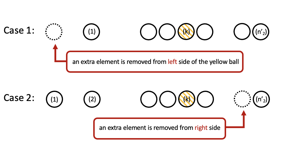
To simplify the notation, let denote in the following discussion. For a fixed , decreasing leads to an increase in and has no effect on the other errors in (14), which means that minimizes . However, the selection of is not as straightforward as . Figure 1(a) illustrates how the set (as appeared in Theorem 1) is constructed for a given , where the elements are ordered by their values. Clearly, more elements are removed from as decreases, leading to a smaller . Consider an element in the set which has rank in the ordered list (colored yellow in Figure 1(a)). Then , and consequently , will all be affected by decreasing , but the change is not monotonic as shown in Figure 1(b). Decreasing could remove elements (dashed circles in Figure 1(b)) either to the left side (case 1) or right side (case 2) of the yellow element, depending on the values of the scores . In case 1, decreases, resulting in a larger and a smaller error, whereas the reverse can happen in case 2. The details of how changes can be found in Supplementary Section B.3, with additional simulations in Supplementary Figure S13. In view of the above, minimizing the empirical error requires a grid search over , for which we use the set , and the overall algorithm for finding the optimal thresholds and the resulting classifier is described in Algorithm 3, which we name as the H-NP umbrella algorithm. The algorithm for the general case with can be found in Supplementary Section E.
2.4 Simulation studies
We first examine the validity of our H-NP umbrella algorithm using simulated data from a setting denoted T1.1, where , and the feature vectors in class are generated as , where , , and is the identity matrix. For each simulated dataset, we generate the feature vectors and labels with 500 observations in each of the three classes. The observations are randomly separated into parts for score training, threshold selection and computing empirical errors: is split into , for , ; is split into , and for , and ; is split into , for , , respectively. All the results in this section are based on repetitions from a given setting. We set and . To approximate and evaluate the true population errors , and , we additionally generate observations for each class and refer to them as the test set.
First, we demonstrate that Algorithm 3 outputs an H-NP classifier with the desired high probability controls. More specifically, we show that any and (, are computed by Algorithm 2) will lead to a valid threshold pair satisfying and , where and are approximated using the test set in each round of simulation. Here, we use multinomial logistic regression to construct the scoring functions and , the inputs of Algorithm 3. Figure 2 displays the boxplots of various approximate errors with chosen as the -th largest element in as changes. In Figure 2(a) and 2(b), where the blue diamonds mark the quantiles, we can see that the violation rate of the required error bounds (red dashed lines, representing and ) is about or less, suggesting our procedure provides effective controls on the errors of concerns. In this case, in most simulation rounds, minimizes the empirical error computed on and , and is chosen as the optimal threshold by Algorithm 3 in the final classifier. We can see this coincide with Figure 2(c), which shows that the largest element in (i.e., ) minimizes the approximate error on the test set. We note here that the results from other splitting ratios can be found in Supplementary Section C.2, where we observe that once the sample size for threshold selection reaches about twice the minimum sample size requirement, there are little observable differences in the results. In Supplementary Section C.3, we also compare with variations in computing the scoring functions to examine the effect of score normalization and calibration, showing that our current scoring functions are ideal for our purpose.
Next, we check whether indeed Theorem 1 gives a better upper bound on than Proposition 1 for overall error minimization. Recall the two upper bounds in Eq (6) () and Eq (9) (). For each base classification algorithm (e.g., logistic regression), we set and equal to these two upper bounds respectively, resulting in two classifiers with different thresholds. We compare their performance by evaluating the approximate errors of and since, as discussed in Section 2.3, the threshold only influences these two errors for a fixed . Figure 3 shows the distributions of the errors and also their averages for three different base classification algorithms. Under each algorithm, both choices of effectively control , but the upper bound from Proposition 1 is overly conservative compared with that of Theorem 1, which results in a notable increase in . This is undesirable since is one component in , and the goal is to minimize under appropriate error controls.
| Logistic Regression | ||
|---|---|---|
| Method | Error23 | Error32 |
| Prop 1 | 0.006 | 0.082 |
| Thm 1 | 0.020 | 0.046 |
| Random Forest | ||
| Method | Error23 | Error32 |
| Prop 1 | 0.004 | 0.077 |
| Thm 1 | 0.017 | 0.033 |
| SVM | ||
| Method | Error23 | Error32 |
| Prop 1 | 0.006 | 0.083 |
| Thm 1 | 0.020 | 0.047 |
Now we consider comparing our H-NP classifier against alternative approaches. We construct an example of “approximate” error control using the empirical ROC curve approach. In this case, each class of observations is split into two parts: one for training the base classification method, the other for threshold selection using the ROC curve. Under the setting T1.1, using similar splitting ratios as before, we separate into and for and for . The same test set is used. We re-compute the scoring functions ( and ) corresponding to the new split. is selected using the ROC curve generated by aiming to distinguish between class 1 (samples in ) and class (samples in ) merging classes 2 and 3, with specificity calculated as the rate of misclassifying a class-1 observation into class . Similarly, is selected using dividing samples in into class 2 and class 3, with specificity defined as the rate of misclassifying a class-2 observation into class 3. More specifically, in Eq (13) we use and to obtain the classifier for the ROC curve approach.
The comparison between our H-NP classifier and the ROC curve approach is summarized in Figure 4. Recalling and are both , we mark the quantiles of the under-classification errors by solid black lines and the target error control levels by dotted red lines. First we observe that the quantiles of using the ROC curve approach well exceed the target level control, with their averages centering around the target. We also see the influence of on the – without suitably adjusting based on , the control on in the ROC curve approach is overly conservative despite it being an approximate error control method, which in turn leads to inflation in error . In view of this, we further consider a simulation setting where the influence of on is smaller. The setting T2.1 moves samples in class 1 further away from classes 2 and 3 by having , while the other parts remain the same as in the setting T1.1. are still . As shown in Figure 5, the ROC curve approach does not provide the required level of control for or .
In Supplementary Sections C.4-C.6, we include more comparisons with alternative methods with different overall approaches to the problem, including weight-adjusted classification, cost-sensitive learning, and ordinal regression, and show that our H-NP framework is more ideal for our problem of interest.

| Logistic Regression | |||
|---|---|---|---|
| Error1 | Error23 | Error32 | |
| Method | ( quantile) | (mean) | |
| ROC | 0.074 | 0.023 | 0.096 |
| H-NP | 0.045 | 0.036 | 0.047 |
| Random Forest | |||
| Error1 | Error23 | Error32 | |
| Method | ( quantile) | (mean) | |
| ROC | 0.077 | 0.020 | 0.093 |
| H-NP | 0.047 | 0.034 | 0.032 |
| SVM | |||
| Error1 | Error23 | Error32 | |
| Method | ( quantile) | (mean) | |
| ROC | 0.078 | 0.023 | 0.098 |
| H-NP | 0.048 | 0.037 | 0.047 |

3 Application to COVID-19 severity classification
3.1 ScRNA-seq data and featurization
We integrate 20 publicly available scRNA-seq datasets to form a total of COVID-19 patients with three severity levels marked as “Severe/Critical” (318 patients), “Mild/Moderate” (353 patients), and “Healthy” (193 patients). The detail of each dataset and patient composition can be found in Supplementary Table S1. The severe, moderate and healthy patients are labeled as class 1, 2 and 3, respectively.
For each patient, PBMC scRNA-seq data is available in the form of a matrix recording the expression levels of genes in hundreds to thousands of cells. Following the workflow in Lin et al. 2022a, we first perform data integration including cell type annotation and batch effect removal, before selecting highly variable genes and constructing their pseudo-bulk expression profiles under each cell type, where each gene’s expression is averaged across the cells of this type in every patient. The resulting processed data for each patient is a matrix , where is the number of cell types, and is the number of genes for analysis. More details of the integration process can be found in Supplementary Section A. Supplementary Figure S1 shows the distribution of the sparsity levels, i.e., the proportion of genes with zero values, under each cell type across all the patients. Several cell types, despite having a significant proportion of zeros, have varying sparsity across the three severity classes (Supplementary Figure S3), suggesting their activity level might be informative for classification. Since age information is available (although in different forms, see Supplementary Table S4) in most of the datasets we integrate, we include it as an additional clinical variable for classification. The details of processing the age variable are deferred to Supplementary Section A.
Since classical classification methods typically use feature vectors as input, appropriate featurization that transforms the expression matrices into vectors is needed. We propose four ways of featurization that differ in their considerations of the following aspects.
- •
As we observe the sparsity level in some cell types changes across the severity classes, we expect different treatments of zeros will influence the classification performance. Three approaches are proposed: 1) no special treatment (M.1); 2) remove individual zeros but keeping all cell types (M.4); 3) remove cell types with significant amount of zeros across all three classes (M.2 and M.3).
- •
Dimension reduction is commonly used to project the information in a matrix onto a vector. We consider performing dimension reduction along different directions, namely row projections, which take combinations of genes (M.2), and column projections, which combine cell types with appropriate weights (M.3 and M.4). We aim to compare choices of projection direction, so we focus on principal component analysis (PCA) as our dimension reduction method.
- •
We consider two approaches to generate the PCA loadings: 1) overall PCA loadings (M.2 and M.4), where we perform PCA on the whole data to output a loading vector for all patients; 2) patient-specific PCA loadings (M.3), where PCA is performed for each matrix to get an individual-specific loading vector.
The details of each featurization method are as follows.
- M.1
Simple feature screening: we consider each element (gene under cell type ) as a possible feature for patient and use its standard deviation across all patients, denoted as , to screen the features. Elements that hardly vary across the patients are likely to have a low discriminative power for classification. Let be the -th largest element in . The feature vector for each patient consists of the entries in , where is the number of features desired and set to .
- M.2
Overall gene combination: removing cell types with mostly zero expression values across all patients (details in Supplementary Section A), we select 17 cell types to construct that only preserves columns in corresponding to the selected cell types. Then, are concatenated column-wise to get , where . Let denote the first principle component loadings of , and the feature vector for patient is given by .
- M.3
Individual-specific cell type combination: for patient , the loading vector is taken as the absolute values of first principle component loadings for , the matrix with selected 17 cell types in M.2 (details in Supplementary Section A). The principle component loading vector that produces is patient-specific, intending to reflect different cell type compositions in different individuals.
- M.4
Common cell type combination: we compute an expression matrix averaged over all patients defined as
where is the cardinality function. Let denote the first principle component loadings of , then the feature vector for the -th patient is .
We next evaluate the performance of these featurizations when applied as input to different base classification methods for H-NP classification.
3.2 Results of H-NP classification
After obtaining the feature vectors and applying a suitable base classification method, we apply Algorithm 3 to control the under-classification errors. Recall that represent the severe, moderate and healthy categories, respectively, and the goal is to control and . In this section, we evaluate the performance of the H-NP classifier applied to each combination of featurization method in Section 3.1 and base classification method (logistic regression, random forest, SVM (linear)), which is used to train the scores ( and ). In each class, we leave out of the data as the test set and split the rest as follows for training the H-NP classifier: and of form and ; , and of form , and ; and of form and . For each combination of featurization and base classification method, we perform random splitting of the observations for 50 times to produce the results in this section.
In Figure 6, the yellow halves of the violin plots show the distributions of different approximate errors from the classical classification methods; Supplementary Table S7 records the averages of these errors. In all the cases, the average of the approximate error is greater than , in many cases greater than . On the other hand, the approximate error under the classical paradigm is already relatively low, with the averages around . Under the H-NP paradigm, we set and , i.e., we want to control each under-classification error under at a tolerance level.
With the prespecified , for a given base classification method Algorithm 3 outputs an H-NP classifier that controls the under-classification errors while minimizing the weighted sum of the other empirical errors. The blue half violin plots in Figure 6 show the resulting approximate errors after H-NP adjustment. We observe that the common cell type combination feature M.4 consistently leads to smaller errors under both the classical and H-NP classifiers, especially for linear classification models (logistic regression and SVM). We have also implemented a neural network classifier. However, as the training sample size is relatively small, its performance is not as good as the linear classification models, and the results are deferred to Supplementary Figure S14.
In each plot of Figure 6, the two leftmost plots are the distributions of the two approximate under-classification errors and . We mark the quantiles of and by short black lines (since ), and the desired control levels () by red dashed lines. The four rightmost plots show the approximate errors for the overall risk and the three components in as discussed in Eq (14). For all the featurization and base classification methods, the under-classification errors are controlled at the desired levels with a slight increase in the overall error, which is much smaller than the reduction in under-classification errors. This demonstrates consistency of our method and indicates its general applicability to various base classification algorithms chosen by users.
Another interesting phenomenon is that when a classical classification method is conservative for specified and , our algorithm will increase the corresponding threshold , which relaxes the decision boundary for classes less prioritized than . As a result, the relaxation will benefit some components in . In Figure 6(d), in many cases the classifier produces an approximate error less than under the classical paradigm, which means it is conservative for the control level at the tolerance level . In this case, the NP classifier adjusts the threshold to lower the requirement for class 3, thus notably decreasing the approximate error of .
3.3 Identifying genomic features associated with severity
Finally, we show that using this integrated scRNA-seq data in a classification setting enables us to identify genomic features associated with disease severity in patients at both the cell-type and gene levels. First, by combining logistic regression with an appropriate featurization, we generate a ranked list of features (i.e., cell types or genes) that are important in predicting severity. At the cell type level, we utilize logistic regression with the featurization M.2, which compresses the expression matrix for each patient into a cell-type-length vector, and rank the cell types based on their coefficients from the log odds ratios of the severe category relative to the healthy category. Supplementary Table S8 shows the top-ranked cell types are CD monocytes, NK cells, CD effector T cells, and neutrophils, all with significant p-values. This is consistent with known involvement of these cell types in the immune response of severe patients (Lucas et al. 2020; Liu et al. 2020; Rajamanickam et al. 2021).
At the gene level, we utilize logistic regression with the featurization M.4, which has the best overall classification performance, and compresses each patient’s expression matrix into a gene-length vector. Similar to the above analysis at the cell-type level, we generate a ranked gene list which leads to the identification of pathways associated with the severe condition. By performing the pathway enrichment analysis on the ranked gene list, we find that the top-ranked genes are significantly enriched in pathways involved in viral defense and leukocyte-mediated immune response (Supplementary Table S9).
Next, we perform further analysis to directly demonstrate the benefits of the H-NP classification results without relying on feature ranking. Based on the featurization M.4, we construct a gene co-expression network and identify modules with groups of genes that are potentially co-regulated and functionally related. By comparing the predicted severity labels from the H-NP classifier and the classical approach, we show that the H-NP labels are better correlated with the eigengenes from these functional modules, suggesting that the H-NP labels better capture the underlying signals in the data related to disease mechanism and immune response (Supplementary Figures S15-S17). Then, we compare the gene ontology enrichment of the functional modules constructed for the severe and healthy patients separately, using the predicted H-NP labels. We find strong evidence of immune response to the virus among severe patients, while no such evidence is observed in the healthy group (Supplementary Tables S10 and S11). Finally, we note that compared with the results from the severe patients as labeled by the classical paradigm, the H-NP paradigm shows more significantly enriched modules with specific references to important cell types, including T cells, and subtypes of T cells (Supplementary Tables S10 and S12). Together, these results demonstrate that by prioritizing the severe category in our H-NP framework, we can uncover stronger biological signals in the data related to immune response.
More detailed descriptions of the methods used and analysis of results can be found in Supplementary Sections D.4 and D.5.
4 Discussion
In general disease severity classification, under-classification errors are more consequential as they can increase the risk of patients receiving insufficient medical care. By assuming the classes have a prioritized ordering, we propose an H-NP classification framework and its associated algorithm (Algorithm 3) capable of controlling under-classification errors at desired levels with high probability. The algorithm performs post hoc adjustment on scoring-type classification methods and thus can be applied in conjunction with most methods preferred by users. The idea of choosing thresholds on the scoring functions based on a held-out set bears resemblance to conformal splitting methods (Lei 2014; Wang and Qiao 2022). However, our approach differs in that we assign only one label to each observation, while maintaining high probability error controls. Additionally, our approach prioritizes certain misclassification errors, unlike conformal prediction which treats all classes equally.
Through simulations and the case study of COVID-19 severity classification, we demonstrate the efficacy of our algorithm in achieving the desired error controls. We have also compared different ways of constructing interpretable feature vectors from the multi-patient scRNA-seq data and shown that the common cell type PCA featurization overall achieves better performance under various classification settings. By performing extensive gene ontology enrichment analysis, we illustrate that the use of scRNA-seq data has allowed us to gain biological insights into the disease mechanism and immune response of severe patients. We note here that although parts of our analysis rely on a ranked feature list obtained from logistic regression, there exist tools to perform such a feature selection step for all the other base classification methods used in this paper, including neural networks, which can utilize saliency maps and other feature selection procedures (Adebayo et al. 2018; Novakovsky et al. 2023). We have chosen logistic regression in our illustrative analysis based on its stable classification performance and ease of interpretation. In addition, if the main objective is to build a classifier for triage diagnostics using other clinical variables, one can easily apply our method to other forms of patient-level COVID-19 data with other base classification methods.
Even though our case study has three classes, the framework and algorithm developed are general. Increasing the number of classes has no effect on the minimum size requirement of the left-out part of each class for threshold selection since it suffices for each class to satisfy . We also note that the notion of prioritized classes can be defined in a context-specific way. For example, in some diseases like Alzheimer’s disease, the transitional stage is considered to be the most important (Xiong et al. 2006).
There are several interesting directions for future work. For small data problems where the minimum sample size requirement is not full-filled, we might consider adopting a parametric model, under which we can not only develop a new algorithm without minimum sample size requirement, but also study the oracle type properties of the classifiers. In terms of featurizing multi-patient scRNA-seq data, we have chosen PCA as the dimension reduction method to focus on other aspects of comparison; more dimension reduction methods can be explored in future work. It is also conceivable that the class labels in the case study are noisy with possibly biased diagnosis. Accounting for label noise with a realistic noise model and extending the work of Yao et al. 2022 to a multi-class NP classification setting will be another interesting direction to pursue.
Acknowledgements
The authors would like to thank the Editor, Associate Editor, and two anonymous reviewers for their valuable comments, which have led to a much improved version of this paper. The authors would also like to thank Dr Yingxin Lin and the Sydney Precision Data Science Centre for their generous help with curating and processing the COVID-19 scRNA-seq data. The authors gratefully acknowledge: the UT Austin Harrington Faculty Fellowship to Y.X.R.W. and NSF DMS-2113754 to J.J.L. and X.T. The authors report there are no competing interests to declare.
References
- World Health Organization [2023] World Health Organization. COVID-19 dashboard, 2023. URL https://covid19.who.int/. Accessed: April 23, 2023.
- Betensky and Feng [2020] Rebecca A Betensky and Yang Feng. Accounting for incomplete testing in the estimation of epidemic parameters. Int J Epidemiol, 49(5):1419–1426, 2020.
- Quick et al. [2021] Corbin Quick, Rounak Dey, and Xihong Lin. Regression models for understanding covid-19 epidemic dynamics with incomplete data. JASA, 116(536):1561–1577, 2021.
- Brooks et al. [2020] Logan C Brooks, Evan L Ray, et al. Comparing ensemble approaches for short-term probabilistic covid-19 forecasts in the us. International Institute of Forecasters, 2020.
- Tang et al. [2021] Francesca Tang, Yang Feng, et al. The interplay of demographic variables and social distancing scores in deep prediction of us covid-19 cases. JASA, 116(534):492–506, 2021.
- McDonald et al. [2021] Daniel J McDonald, Jacob Bien, et al. Can auxiliary indicators improve covid-19 forecasting and hotspot prediction? PNAS, 118(51), 2021.
- James et al. [2021] Nick James, Max Menzies, and Peter Radchenko. Covid-19 second wave mortality in europe and the united states. Chaos, 31(3):031105, 2021.
- Kramlinger et al. [2022] Peter Kramlinger, Tatyana Krivobokova, and Stefan Sperlich. Marginal and conditional multiple inference for linear mixed model predictors. JASA, 0(ja):1–31, 2022. doi: 10.1080/01621459.2022.2044826. URL https://doi.org/10.1080/01621459.2022.2044826.
- Wu et al. [2020] Jiangpeng Wu, Pengyi Zhang, et al. Rapid and accurate identification of covid-19 infection through machine learning based on clinical available blood test results. MedRxiv, 2020.
- Li et al. [2020] Wei Tse Li, Jiayan Ma, et al. Using machine learning of clinical data to diagnose covid-19: a systematic review and meta-analysis. BMC Med Inform Decis Mak, 20(1):1–13, 2020.
- Zhang et al. [2021] Jiawei Zhang, Jie Ding, and Yuhong Yang. Is a classification procedure good enough?—a goodness-of-fit assessment tool for classification learning. JASA, pages 1–11, 2021.
- Yan et al. [2020] Li Yan, Hai-Tao Zhang, et al. Prediction of criticality in patients with severe covid-19 infection using three clinical features: a machine learning-based prognostic model with clinical data in wuhan. MedRxiv, 27:2020, 2020.
- Sun et al. [2020] Liping Sun, Fengxiang Song, et al. Combination of four clinical indicators predicts the severe/critical symptom of patients infected covid-19. J. Clin. Virol, 128:104431, 2020.
- Zhao et al. [2020] Zirun Zhao, Anne Chen, et al. Prediction model and risk scores of icu admission and mortality in covid-19. PloS one, 15(7):e0236618, 2020.
- Ortiz et al. [2022] Anthony Ortiz, Anusua Trivedi, et al. Effective deep learning approaches for predicting covid-19 outcomes from chest computed tomography volumes. Sci Rep, 12(1):1–10, 2022.
- Alballa and Al-Turaiki [2021] Norah Alballa and Isra Al-Turaiki. Machine learning approaches in covid-19 diagnosis, mortality, and severity risk prediction: A review. IMU, 24:100564, 2021.
- Meraihi et al. [2022] Yassine Meraihi, Asma Benmessaoud Gabis, et al. Machine learning-based research for covid-19 detection, diagnosis, and prediction: A survey. SN computer science, 3(4):286, 2022.
- Overmyer et al. [2021] Katherine A Overmyer, Evgenia Shishkova, et al. Large-scale multi-omic analysis of covid-19 severity. Cell Syst., 12(1):23–40, 2021.
- Wilk et al. [2020] Aaron J Wilk, Arjun Rustagi, et al. A single-cell atlas of the peripheral immune response in patients with severe covid-19. Nat. Med., 26(7):1070–1076, 2020.
- Stephenson et al. [2021] Emily Stephenson, Gary Reynolds, et al. Single-cell multi-omics analysis of the immune response in covid-19. Nat. Med., 27(5):904–916, 2021.
- Ren et al. [2021] Xianwen Ren, Wen Wen, et al. Covid-19 immune features revealed by a large-scale single-cell transcriptome atlas. Cell, 184(7):1895–1913, 2021.
- Aibar et al. [2015] Sara Aibar, Celia Fontanillo, et al. Analyse multiple disease subtypes and build associated gene networks using genome-wide expression profiles. BMC genomics, 16:1–10, 2015.
- Arvaniti and Claassen [2017] Eirini Arvaniti and Manfred Claassen. Sensitive detection of rare disease-associated cell subsets via representation learning. Nat. Commun., 8(1):1–10, 2017.
- Hu et al. [2019] Zicheng Hu, Benjamin S Glicksberg, and Atul J Butte. Robust prediction of clinical outcomes using cytometry data. Bioinformatics, 35(7):1197–1203, 2019.
- World Health Organization [2020] World Health Organization. Who r&d blueprint novel coronavirus covid-19 therapeutic trial synopsis. World Health Organization, pages 1–9, 2020.
- Tong et al. [2018] Xin Tong, Yang Feng, and Jingyi Jessica Li. Neyman-pearson classification algorithms and np receiver operating characteristics. Sci. Adv., 4(2):eaao1659, 2018.
- Lin et al. [2022a] Yingxin Lin, Lipin Loo, et al. Scalable workflow for characterization of cell-cell communication in covid-19 patients. PLoS Comp Biol, 18(10):e1010495, 2022a.
- Meyer and Pauker [1987] Klemens B Meyer and Stephen G Pauker. Screening for hiv: can we afford the false positive rate?, 1987.
- Dettling and Bühlmann [2003] Marcel Dettling and Peter Bühlmann. Boosting for tumor classification with gene expression data. Bioinformatics, 19(9):1061–1069, 2003.
- Elkan [2001] Charles Elkan. The foundations of cost-sensitive learning. In International joint conference on artificial intelligence, volume 17, pages 973–978. Lawrence Erlbaum Associates Ltd, 2001.
- Margineantu [2002] Dragos D Margineantu. Class probability estimation and cost-sensitive classification decisions. In Machine Learning: ECML 2002: 13th European Conference on Machine Learning Helsinki, Finland, August 19–23, 2002 Proceedings 13, pages 270–281. Springer, 2002.
- Cannon et al. [2002] Adam Cannon, James Howse, et al. Learning with the neyman-pearson and min-max criteria. Los Alamos National Laboratory, Tech. Rep. LA-UR, pages 02–2951, 2002.
- Scott and Nowak [2005] Clayton Scott and Robert Nowak. A neyman-pearson approach to statistical learning. IEEE Trans. Inf. Theory, 51(11):3806–3819, 2005.
- Rigollet and Tong [2011] Philippe Rigollet and Xin Tong. Neyman-pearson classification, convexity and stochastic constraints. JMLR, 2011.
- Xia et al. [2021] Lucy Xia, Richard Zhao, et al. Intentional control of type i error over unconscious data distortion: A neyman–pearson approach to text classification. JASA, 116(533):68–81, 2021.
- Feng et al. [2021] Yang Feng, Xin Tong, and Weining Xin. Targeted crisis risk control: A neyman-pearson approach. Available at SSRN 3945980, 2021.
- Landgrebe and Duin [2005] Thomas Landgrebe and R Duin. On neyman-pearson optimisation for multiclass classifiers. In Proceedings 16th Annual Symposium of the Pattern Recognition Association of South Africa. PRASA, pages 165–170, 2005.
- Xiong et al. [2006] Chengjie Xiong, Gerald van Belle, et al. Measuring and estimating diagnostic accuracy when there are three ordinal diagnostic groups. Statistics in Medicine, 25(7):1251–1273, 2006.
- Tian and Feng [2021] Ye Tian and Yang Feng. Neyman-pearson multi-class classification via cost-sensitive learning. arXiv preprint arXiv:2111.04597, 2021.
- Stanley et al. [2020] Natalie Stanley, Ina A Stelzer, et al. Vopo leverages cellular heterogeneity for predictive modeling of single-cell data. Nat. Commun., 11(1):1–9, 2020.
- Ganio et al. [2020] Edward A Ganio, Natalie Stanley, et al. Preferential inhibition of adaptive immune system dynamics by glucocorticoids in patients after acute surgical trauma. Nat. Commun., 11(1):1–12, 2020.
- Han et al. [2019] Xiaoyuan Han, Mohammad S Ghaemi, et al. Differential dynamics of the maternal immune system in healthy pregnancy and preeclampsia. Front Immunol., page 1305, 2019.
- Davis et al. [2017] Mark M Davis, Cristina M Tato, and David Furman. Systems immunology: just getting started. Nat. Immunol., 18(7):725–732, 2017.
- Lucas et al. [2020] Carolina Lucas, Patrick Wong, et al. Longitudinal analyses reveal immunological misfiring in severe covid-19. Nature, 584(7821):463–469, 2020.
- Liu et al. [2020] Jing Liu, Sumeng Li, et al. Longitudinal characteristics of lymphocyte responses and cytokine profiles in the peripheral blood of sars-cov-2 infected patients. EBioMedicine, 55:102763, 2020.
- Rajamanickam et al. [2021] Anuradha Rajamanickam, Nathella Pavan Kumar, et al. Dynamic alterations in monocyte numbers, subset frequencies and activation markers in acute and convalescent covid-19 individuals. Sci. Rep., 11(1):20254, 2021.
- Lei [2014] Jing Lei. Classification with confidence. Biometrika, 101(4):755–769, 2014.
- Wang and Qiao [2022] Wenbo Wang and Xingye Qiao. Set-valued support vector machine with bounded error rates. JASA, pages 1–13, 2022.
- Adebayo et al. [2018] Julius Adebayo, Justin Gilmer, et al. Sanity checks for saliency maps. NeurIPS, 31, 2018.
- Novakovsky et al. [2023] Gherman Novakovsky, Nick Dexter, et al. Obtaining genetics insights from deep learning via explainable artificial intelligence. Nat. Rev. Genet., 24(2):125–137, 2023.
- Yao et al. [2022] Shunan Yao, Bradley Rava, et al. Asymmetric error control under imperfect supervision: A label-noise-adjusted neyman–pearson umbrella algorithm. JASA, pages 1–13, 2022.
- McCarthy et al. [2017] Davis J McCarthy, Kieran R Campbell, et al. Scater: pre-processing, quality control, normalization and visualization of single-cell rna-seq data in r. Bioinformatics, 33(8):1179–1186, 2017.
- Lin et al. [2022b] Yingxin Lin, Yue Cao, et al. Atlas-scale single-cell multi-sample multi-condition data integration using scmerge2. bioRxiv, pages 2022–12, 2022b.
- Lin et al. [2020] Yingxin Lin, Yue Cao, et al. scclassify: sample size estimation and multiscale classification of cells using single and multiple reference. Mol Syst Biol, 16(6):e9389, 2020.
- Lun et al. [2016] Aaron TL Lun, Davis J McCarthy, and John C Marioni. A step-by-step workflow for low-level analysis of single-cell rna-seq data with bioconductor. F1000Research, 5, 2016.
- Arunachalam et al. [2020] Prabhu S Arunachalam, Florian Wimmers, et al. Systems biological assessment of immunity to mild versus severe covid-19 infection in humans. Science, 369(6508):1210–1220, 2020.
- Bost et al. [2021] Pierre Bost, Francesco De Sanctis, et al. Deciphering the state of immune silence in fatal covid-19 patients. Nat. Commun., 12(1):1428, 2021.
- COMBAT et al. [2021] COMBAT, David J Ahern, et al. A blood atlas of covid-19 defines hallmarks of disease severity and specificity. MedRxiv, pages 2021–05, 2021.
- Combes et al. [2021] Alexis J Combes, Tristan Courau, et al. Global absence and targeting of protective immune states in severe covid-19. Nature, 591(7848):124–130, 2021.
- Lee et al. [2020] Jeong Seok Lee, Seongwan Park, et al. Immunophenotyping of covid-19 and influenza highlights the role of type i interferons in development of severe covid-19. Sci Immunol, 5(49):eabd1554, 2020.
- Liu et al. [2021] Can Liu, Andrew J Martins, et al. Time-resolved systems immunology reveals a late juncture linked to fatal covid-19. Cell, 184(7):1836–1857, 2021.
- Ramaswamy et al. [2021] Anjali Ramaswamy, Nina N Brodsky, et al. Immune dysregulation and autoreactivity correlate with disease severity in sars-cov-2-associated multisystem inflammatory syndrome in children. Immunity, 54(5):1083–1095, 2021.
- Schulte-Schrepping et al. [2020] Jonas Schulte-Schrepping, Nico Reusch, et al. Severe covid-19 is marked by a dysregulated myeloid cell compartment. Cell, 182(6):1419–1440, 2020.
- Schuurman et al. [2021] Alex R Schuurman, Tom DY Reijnders, et al. Integrated single-cell analysis unveils diverging immune features of covid-19, influenza, and other community-acquired pneumonia. Elife, 10:e69661, 2021.
- Silvin et al. [2020] Aymeric Silvin, Nicolas Chapuis, et al. Elevated calprotectin and abnormal myeloid cell subsets discriminate severe from mild covid-19. Cell, 182(6):1401–1418, 2020.
- Sinha et al. [2022] Sarthak Sinha, Nicole L Rosin, et al. Dexamethasone modulates immature neutrophils and interferon programming in severe covid-19. Nat. Med., 28(1):201–211, 2022.
- Su et al. [2020] Yapeng Su, Daniel Chen, et al. Multi-omics resolves a sharp disease-state shift between mild and moderate covid-19. Cell, 183(6):1479–1495, 2020.
- Thompson et al. [2021] Elizabeth A Thompson, Katherine Cascino, et al. Metabolic programs define dysfunctional immune responses in severe covid-19 patients. Cell reports, 34(11):108863, 2021.
- Unterman et al. [2022] Avraham Unterman, Tomokazu S Sumida, et al. Single-cell multi-omics reveals dyssynchrony of the innate and adaptive immune system in progressive covid-19. Nat. Commun., 13(1):440, 2022.
- Yao et al. [2021] Changfu Yao, Stephanie A Bora, et al. Cell-type-specific immune dysregulation in severely ill covid-19 patients. Cell reports, 34(1):108590, 2021.
- Zhao et al. [2021] Xiang-Na Zhao, Yue You, et al. Single-cell immune profiling reveals distinct immune response in asymptomatic covid-19 patients. Signal Transduct Target Ther, 6(1):342, 2021.
- Zhu et al. [2020] Linnan Zhu, Penghui Yang, et al. Single-cell sequencing of peripheral mononuclear cells reveals distinct immune response landscapes of covid-19 and influenza patients. Immunity, 53(3):685–696, 2020.
- Zadrozny and Elkan [2002] Bianca Zadrozny and Charles Elkan. Transforming classifier scores into accurate multiclass probability estimates. In Proceedings of the eighth ACM SIGKDD international conference on Knowledge discovery and data mining, pages 694–699, 2002.
- Agresti [2002] Alan Agresti. Categorical data analysis second edition, 2002.
- Hornung [2020] Roman Hornung. Ordinal forests. J Classif, 37:4–17, 2020.
- Frank and Hall [2001] Eibe Frank and Mark Hall. A simple approach to ordinal classification. In Machine Learning: ECML 2001: 12th European Conference on Machine Learning Freiburg, Germany, September 5–7, 2001 Proceedings 12, pages 145–156. Springer, 2001.
- Cardoso and da Costa [2007] Jaime Cardoso and Joaquim Pinto da Costa. Learning to classify ordinal data: The data replication method. JMLR, 2007.
- Ma and Ahn [2021] Ziyang Ma and Jeongyoun Ahn. Feature-weighted ordinal classification for predicting drug response in multiple myeloma. Bioinformatics, 37(19):3270–3276, 2021.
- Moussa and Măndoiu [2018] Marmar Moussa and Ion I Măndoiu. Single cell rna-seq data clustering using tf-idf based methods. BMC genomics, 19(6):31–45, 2018.
- Korotkevich et al. [2016] Gennady Korotkevich, Vladimir Sukhov, et al. Fast gene set enrichment analysis. BioRxiv, page 060012, 2016.
- Peng et al. [2020] Yanchun Peng, Alexander J Mentzer, et al. Broad and strong memory cd4+ and cd8+ t cells induced by sars-cov-2 in uk convalescent individuals following covid-19. Nat Immunol., 21(11):1336–1345, 2020.
- Zhang and Horvath [2005] Bin Zhang and Steve Horvath. A general framework for weighted gene co-expression network analysis. Stat Appl Genet Mol Biol, 4(1), 2005.
- Langfelder and Horvath [2014] Peter Langfelder and Steve Horvath. Tutorials for the wgcna package. UCLA. Los Ageles, 2014.
- Wu et al. [2021] Tianzhi Wu, Erqiang Hu, et al. clusterprofiler 4.0: A universal enrichment tool for interpreting omics data. The Innovation, 2(3):100141, 2021.
- Huang et al. [2020] Chaolin Huang, Yeming Wang, et al. Clinical features of patients infected with 2019 novel coronavirus in wuhan, china. The lancet, 395(10223):497–506, 2020.
- Que et al. [2022] Yifan Que, Chao Hu, et al. Cytokine release syndrome in covid-19: a major mechanism of morbidity and mortality. Int Rev Immunol, 41(2):217–230, 2022.
A Preprocessing of the integrated COVID-19 data
We integrate 20 collections of scRNA-seq datasets from peripheral blood mononuclear cells (PBMCs). A total of 864 patients are available and their severity levels can be found in Table S1. Table S2 summarizes populations and geographic locations covered by the datasets. We note that some of these datasets contain patients with longitudinal records; we take only one sample from these multiple measurements to ensure independence.
Before integration, we performed size factor standardization and log transformation on the raw count expression matrices using the logNormCount function in the R package scater (version 1.16.2) [McCarthy et al. 2017] and generated log transformed gene expression matrices. All the PBMC datasets are integrated by scMerge2 [Lin et al. 2022b], which is specifically designed for merging multi-sample and multi-condition studies. Following the standard pipeline for assessing the quality of integration, in Figure S2, we show the UMAP projections of all cells from all the studies, obtained from the top 20 principle components of the merged gene-by-cell expression matrix, for (a) before integration and (b) after integration. The cells are colored by their cell types (left column) or which study (or batch) they come from (right column). Before integration, cells from the same cell type are split into separate clusters based on batch labels, indicating the presence of batch effects. After integration, cells from the same cell type are significantly better mixed while the distinctions among cell types are preserved.
To construct pseudo-bulk expression profiles, we input the cell types annotated by scClassify [Lin et al. 2020] (using cell types in Stephenson et al. 2021 as reference) into scMerge2. The resulting profiles are used to identify mutual nearest subgroups as pseudo-replicates and to estimate parameters of the scMerge2 model. We select the top highly variable genes through the function modelGeneVar in R package scran [Lun et al. 2016], and for each patient calculate the average expression of each cell type for selected genes, i.e., for each patient, the integrated dataset provides a matrix recording the average gene expressions, where is the number of genes () and is the number of cell types ().
| Publication | Severe/Critical | Mild/Moderate | Healthy | Total |
|---|---|---|---|---|
| Arunachalam et al. 2020 | 4 | 3 | 5 | 12 |
| Bost et al. 2021 | 21 | 6 | 5 | 32 |
| COMBAT et al. 2021 | 62 | 31 | 10 | 103 |
| Combes et al. 2021 | 9 | 11 | 14 | 34 |
| Lee et al. 2020 | 3 | 4 | 5 | 12 |
| Liu et al. 2021 | 30 | 3 | 14 | 47 |
| Ramaswamy et al. 2021* | - | - | 19 | 19 |
| Ren et al. 2021 | 70 | 61 | 20 | 151 |
| Schulte-Schrepping et al. 2020 | 17 | 19 | 38 | 74 |
| Schuurman et al. 2021 | 2 | 6 | 4 | 12 |
| Silvin et al. 2020 | 5 | 2 | 3 | 10 |
| Sinha et al. 2022 | 21 | - | - | 21 |
| Stephenson et al. 2021 | 28 | 53 | 32 | 113 |
| Su et al. 2020 | 12 | 117 | - | 129 |
| Thompson et al. 2021 | 5 | - | 3 | 8 |
| Unterman et al. 2022* | 10 | - | - | 10 |
| Wilk et al. 2020 | 11 | 20 | 8 | 39 |
| Yao et al. 2021 | 6 | 5 | - | 11 |
| Zhao et al. 2021 | 1 | 8 | 10 | 19 |
| Zhu et al. 2020 | 1 | 4 | 3 | 8 |
| Total | 318 | 353 | 193 | 864 |
| Publication | Population | Country |
|---|---|---|
| Arunachalam et al. 2020 | Black, Caucasian | US |
| Bost et al. 2021 | - | Italy |
| COMBAT et al. 2021 | - | UK |
| Combes et al. 2021 | - | US |
| Lee et al. 2020 | - | South Korea |
| Liu et al. 2021 | Asian, Caucasian | Italy |
| Ramaswamy et al. 2021 | - | US |
| Ren et al. 2021 | Asian | China |
| Schulte-Schrepping et al. 2020 | - | Germany |
| Schuurman et al. 2021 | Black, Caucasian | Netherlands |
| Silvin et al. 2020 | - | France |
| Sinha et al. 2022 | Asian, Black, Caucasian, Others | Canada |
| Stephenson et al. 2021 | - | UK |
| Su et al. 2020 | Asian, Black, Caucasian, Others | US |
| Thompson et al. 2021 | - | US |
| Unterman et al. 2022 | - | US |
| Wilk et al. 2020 | Asian, Black, Caucasian, Hispanic/Latino, Others | US |
| Yao et al. 2021 | Asian, Black, Caucasian, Hispanic/Latino, Others | US |
| Zhao et al. 2021 | - | China |
| Zhu et al. 2020 | Asian | China |
In the featurization methods M.2 and M.3, we remove the cell type ILC with its zero proportion hardly changing across all three classes (Figure S3) and an average zero proportion greater than (Table S3). 17 cell types are left: B, CD14 Mono, CD16 Mono, CD4 T, CD8 T, DC,gdT, HSPC, MAST, Neutrophil, NK, NKT, Plasma, Platelet, RBC, DN, MAIT. Also, in M.3, we find that using the absolute values of PCA loadings notably increase the prediction performance under the classical paradigm (even though it is still not as good as M.4).
| cell type | zero proportion | cell type | zero proportion |
|---|---|---|---|
| B | 0.054 | Neutrophil | 0.514 |
| CD14 Mono | 0.028 | NK | 0.025 |
| CD16 Mono | 0.142 | NKT | 0.099 |
| CD4 T | 0.024 | Plasma | 0.243 |
| CD8 T | 0.042 | Platelet | 0.232 |
| DC | 0.186 | RBC | 0.730 |
| gdT | 0.209 | DN | 0.524 |
| HSPC | 0.548 | MAIT | 0.220 |
| MAST | 0.786 | ILC | 0.972 |


Other than scRNA-seq data, we also include age as a predictor in the integrated dataset. Most of the datasets used in our study recorded age information either as an exact number or an age group, while the rest did not provide this information (see Table S4). In the integrated dataset, we use the lower end of the age group recorded for patients with no exact age, and replace the missing values with the average age (52.23).
| Publication | Age recording format | Example |
|---|---|---|
| Arunachalam et al. 2020 | exact age | 64 |
| Bost et al. 2021 | not available | NA |
| COMBAT et al. 2021 | age group | 61-70 |
| Combes et al. 2021 | exact age | 64 |
| Lee et al. 2020 | exact age | 64 |
| Liu et al. 2021 | exact age | 64 |
| Ramaswamy et al. 2021 | exact age | 64 |
| Ren et al. 2021 | exact age | 64 |
| Schulte-Schrepping et al. 2020 | age group | 61-65 |
| Schuurman et al. 2021 | exact age | 64 |
| Silvin et al. 2020 | exact age | 64 |
| Sinha et al. 2022 | exact age | 64 |
| Stephenson et al. 2021 | age group | 60-69 |
| Su et al. 2020 | exact age | 64 |
| Thompson et al. 2021 | not available | NA |
| Unterman et al. 2022 | exact age | 64 |
| Wilk et al. 2020 | age group | 60-69 |
| Yao et al. 2021 | not available | NA |
| Zhao et al. 2021 | exact age | 64 |
| Zhu et al. 2020 | exact age | 64 |
B Proofs of the main results
B.1 Proof of Proposition 1
Recall that , and are the order statistics, with being the cardinality of . Let be the -th order statistic. Suppose is the classification score of an independent observation from class , and is the cumulative distribution function for . Then,
and
| (S.1) |
The inequality holds because , and it becomes an equality when is continuous.
B.2 Proof of Theorem 1
Given , recall that and are the -th order statistic of the sets
respectively, where is the left-out class- samples, and are the thresholds for the previous decisions in the classifier (3). and are the cardinalities of and . Obviously, . Also, we set
where and are the prespecified control level and violation tolerance level, and are the adjusted counterparts, and . With the adjusted and , we consider the following two cases when selecting the upper bound of threshold:
| (S.2) |
where We are going to prove that by two cases.
Case 1: We consider the set (case 1 in Eq (S.2)). Under this event, and we want to show that
Suppose that is the classification score of an independent observation from class . is the cumulative distribution function for the classification score when . Then, similar to the proof of Proposition 1,
Note that is determined by , , . Meanwhile, is fixed, as it only depends on the given values and . We have
| (S.3) |
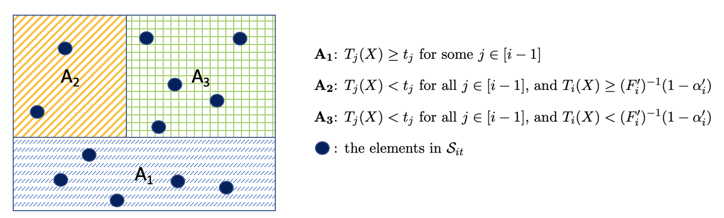
Note that the event indicates that elements in satisfy ; among these elements, at least elements have less than . We can consider as independent draws from a multinomial distribution with three kinds of outcomes () defined in Supplementary Figure S4.
Therefore,
Then, by Eq (B.2),
The last inequality holds because
and it becomes an equality when is continuous.
Also,
since . Then,
| (S.4) | ||||
On the other hand, note that the event is equivalent to
| (S.5) |
and
| (S.6) |
The left part of the inequality (S.6) is decreasing with respect to . Also, the left part of the inequality (S.5) is nonincreasing in when the inequality (S.6) holds, which implies that
i.e., . Immediately,
so
The last inequality is by Hoeffding’s inequality. Then,
| (S.7) |
B.3 The change of in Figure 1b
In the end of Section 2.3, we discuss the selection of and to minimize . Recall that denotes the position of yellow ball (in ) in Figure 1b; and are the adjusted control level and violation tolerance for the second under-classification error ; is the cardinality of . , and are functions of . In the following discussion, we will show that the change in with respect to changing is not monotonic.
We consider a random variable . We abbreviate and . Note that . We will explore how the change of (i.e., the change of ) affect the value of . The following lemma discusses the changes in case 1 of Figure 1b.
Lemma 1.
Let , where for some positive constant and , then .
Proof.
Let , where and are independent. Then, and
| (S.9) |
Also, for fixed and , we have
Therefore, there exists a constant such that
| (S.10) |
Note that . Then,
∎
Note that
Since is fixed, we can write in the form of for some positive constants and . In other words, if we remove an element to the left of the yellow element in Figure 1b case 1, the value of ) will decrease.
By contrast, there are situations in case 2 of Figure 1b that will increase , as discussed in the following lemma.
Lemma 2.
Let , where and . Fix , is decreasing with respect to where .
Proof.
Eq (S.9) implies
| (S.11) |
On the other hand, for fixed and ,
| (S.12) |
so is decreasing on when . Then, according to Eq (S.10)
| (S.13) |
Furthermore,
is increasing in , i.e, any satisfies . It establishes that is decreasing with respect to when . ∎
This lemma presents a situation for case 2 in Figure 1b, where will increase.
C Additional results for simulation studies
C.1 Summary of simulation settings
In the simulation studies, we consider and the feature vectors in class are generated as . The following simulation settings are used throughout the paper:
- •
Setting T1.1: , , , . When applying the H-NP method, the observations are randomly separated into parts for score training, threshold selection, and computing empirical errors: is split into , for , ; is split into , and for , and ; is split into , for , , respectively.
- •
Setting T2.1: , , , . The data splitting is the same as in the setting T1.1 when applying the H-NP method.
- •
Setting T3.1: . , , and . The data splitting is the same as in the setting T1.1 when applying the H-NP method.
All the results in the simulation studies are based on 1,000 repetitions from a given setting. To approximate and evaluate the true population errors, we additionally generate observations as the test set. The ratio of the three classes in the test set is the same as .
We further consider simulation settings T1.2-T1.7, which are variations of T1.1 with the same values of . The details of these simulation settings can be found in Table S5. In the following subsections, these settings allow us to investigate the impact of different splitting settings, score functions, and imbalanced class sizes on the performance of our H-NP classifier. We also compare the performance of our method with cost-sensitive learning, ordinal classification and weight-adjusted classification.
| Class | 1 | 2 | 3 | ||||||||
| Setting | Method | (%) | (%) | (size) | (%) | (%) | (%) | (size) | (%) | (%) | (size) |
| Basic setting | |||||||||||
| T1.1 | classical | 100 | - | 100 | - | - | 100 | - | |||
| H-NP | 50 | 50 | 45 | 50 | 5 | 95 | 5 | ||||
| T1.2 | classical | 100(90,10) | - | 100(90,10) | - | - | 100(90,10) | - | |||
| H-NP | 50(40,10) | 50 | 45(35,10) | 50 | 5 | 95(85,10) | 5 | ||||
| Different splitting ratios (smaller ) | |||||||||||
| T1.3 | H-NP | 80 | 20 | 75 | 20 | 5 | 95 | 5 | |||
| T1.4 | H-NP | 70 | 30 | 65 | 30 | 5 | 95 | 5 | |||
| T1.5 | H-NP | 60 | 40 | 55 | 40 | 5 | 95 | 5 | |||
| Different splitting ratios (larger ) | |||||||||||
| T1.6 | H-NP | 30 | 70 | 25 | 70 | 5 | 95 | 5 | |||
| Imbalanced class sizes | |||||||||||
| T1.7 | classical | 100 | - | 500 | 100 | - | - | 500 | 100 | - | |
| H-NP | 50 | 50 | 500 | 45 | 50 | 5 | 500 | 95 | 5 | ||
C.2 The influence of different splitting settings
We compare different splitting ratios in simulation settings T1.3-T1.6, assigning larger or smaller proportions of the data to select thresholds (see Table S5 for more details).
Under the settings T1.6 (larger threshold sets) and T1.4 (smaller threshold sets), Figures S5 and S6 and show similar trends as Figure 2 in the main paper. As the minimum sample size requirement on is in this case, the setting in Figure 2 already exceeds the requirement. Further increasing its size makes minimal difference in the performance of the H-NP classifier.
Figure S7 shows a comprehensive comparison of settings T1.3-1.5 and the basic setting T1.1, which demonstrate that again these splitting ratios lead to no notable changes. We note that the setting T1.3 only assigns 100 samples to each threshold selection set , which is about twice the minimum sample size requirement.
C.3 Variations in calculating the scoring functions
As mentioned in Section 2.2, we have normalized each scoring function by the factor , motivated by the NP lemma. To illustrate the benefit of normalization empirically, we compare the performance of the normalized scoring functions, , with that of the non-normalized ones, , under the simulation setting T1.1 (see Table S5 for details), the same setting that generated Figure 5 in the main paper. Figure S8 shows the results for two sets of values. Both scoring functions effectively control the under-classification errors, namely “error1” and “error23”, below the desired levels. However, the non-normalized approach controls “error23” in a conservative manner, which results in higher values of “error32” (i.e., ). The other errors not depicted in the plots do not exhibit any noticeable differences.


Next, we note that for general machine learning models such as the random forest and SVM, a probability calibration procedure is often applied to “correct” the output scores for more accurate predicted probabilities. Under the setting T1.1, we compare the original scores from each base classifier with the calibrated scores calculated by the function CalibratedClassifierCV [Zadrozny and Elkan 2002] in the Python package sklearn. The latter is denoted as T1.2 in Table S5, where 10% of each dataset was used for calibration. Figure S9 shows the effect of calibration for all the errors under two different sets of values. Little differences can be seen for logistic regression and random forest. For SVM, the scores with no calibration perform better in , and . In all cases, the H-NP approach maintains effective control over the under-classification errors, regardless of the type of scores used.


C.4 Imbalanced class sizes and weight-adjusted classification
Imbalanced class sizes can lead to more difficulty in controlling prioritized errors. To investigate this effect, we consider the simulation setting T1.7 (with sample sizes of , see Table S5), where the prioritized classes have smaller sample sizes. We compare the results from the classical, H-NP, and weight-adjusted paradigms, where heavier weights are assigned to classes 1 and 2 when computing the empirical loss during optimization.
Table S6 shows the averages of the approximate errors and the relevant quantiles based on our chosen tolerance levels, with visualizations provided in Figure S10. As expected, the imbalanced setting significantly increased the under-classification errors under the classical paradigm compared with the balanced setting. We implemented H-NP with two sets of values, and in both settings the under-classification errors are effectively controlled under the specified levels.
| Logistic Regression | ||||
|---|---|---|---|---|
| Paradigm | Error1 | Error23 | Overall | |
| classical | mean | 0.491 | 0.176 | 0.264 |
| 90% quantile | 0.509 | 0.188 | ||
| 80% quantile | 0.504 | 0.184 | ||
| 70% quantile | 0.499 | 0.181 | ||
| H-NP | mean | 0.075 | 0.058 | 0.464 |
| 90% quantile | 0.098 | 0.077 | ||
| weight | mean | 0.135 | 0.007 | 0.466 |
| 80:50:1 | 90% quantile | 0.145 | 0.010 | |
| H-NP | mean | 0.179 | 0.149 | 0.35 |
| 80% quantile | 0.199 | 0.167 | ||
| weight | mean | 0.203 | 0.032 | 0.36 |
| 15:12:1 | 80% quantile | 0.211 | 0.036 | |
| Random Forest | ||||
| Paradigm | Error1 | Error23 | Overall | |
| classical | mean | 0.489 | 0.184 | 0.271 |
| 90% quantile | 0.529 | 0.213 | ||
| 80% quantile | 0.514 | 0.202 | ||
| 70% quantile | 0.504 | 0.195 | ||
| H-NP | mean | 0.075 | 0.056 | 0.468 |
| 90% quantile | 0.098 | 0.074 | ||
| weight | mean | 0.139 | 0.002 | 0.538 |
| 15:10:1 | 90% quantile | 0.158 | 0.006 | |
| H-NP | mean | 0.178 | 0.148 | 0.354 |
| 80% quantile | 0.198 | 0.167 | ||
| weight | mean | 0.203 | 0.045 | 0.365 |
| 4:4:1 | 80% quantile | 0.223 | 0.053 | |
When choosing the weights for the weight-adjusted paradigm, we note that there is no direct correspondence between the weights and our parameters . For a fair comparison, we performed a grid search on the weights to find weight combinations that led to an overall error roughly similar to that of the H-NP classifier. The grid search is computationally intensive, and the weights are more difficult to interpret than and . Table S6 and Figure S10 show the matched H-NP and weight-adjusted classifications as pairs adjacent to each other for easy comparison. We find that significantly different weights are needed for logistic regression and random forest to achieve similar under-diagnostic errors, suggesting that the choice of weights is not robust across different base classifiers, while the H-NP method is much more consistent. At similar overall error levels, the weight-adjusted classification gives higher , while the control on is more conservative.
C.5 Comparing with cost-sensitive learning
Cost-sensitive learning is an alternative approach to asymmetric error control. However, the costs assigned to different types of errors can be less interpretable and harder to select from a practitioner’s perspective (especially in the multi-class setting) than our parameters and , which represent an upper bound on error rate and a tolerance level in probability, respectively. To perform numerical comparisons, we first note that there is no direct correspondence between our values and the error costs. The only work we are aware of connecting the multi-class NP (NPMC) problem with cost-sensitive learning is Feng et al. 2021. Different from our problem setting, the NPMC method controls and at levels and by computing the appropriate cost assignment. Since is a sum of and , for a fairer comparison, we set the control levels in NPMC and H-NP to be . We compared NPMC and H-NP under the simulation setting T1.1 (details in Table S5) for feasible choices . Setting for NPMC and , , and for H-NP, Figure S11 shows the distributions of the approximate under-classification errors from logistic regression and SVM, with the red dashed lines representing the 90% quantiles. The distributions of highlight the difference between the approximate control by NPMC and the high probability control by H-NP. The NPMC’s control on appears to be slightly more conservative, resulting in slightly higher values.
C.6 Comparison with ordinal classification
We conduct comparisons with ordinal classification methods, including:
- •
cumulative link models (CLMs), which are a type of generalized linear models that use cumulative probabilities to characterize ordinal outcomes. We include both the logit and probit link functions [Agresti 2002], denoted as CLM (logit/probit) in the results below. We also include the method from [Hornung 2020] denoted as ordinalForest, which uses a similar approach using the probit link function but based on random forest;
- •
methods based on decomposing the multi-class classification problem into multiple binary classification problems. We compare with the method FH01 from Frank and Hall 2001, which combines the results from binary classifiers for classes versus classes , and the method oSVM from Cardoso and da Costa 2007, which considers the binary classification problem of classes versus classes for some fixed constant . We use logistic regression and support vector machine (SVM) as the classifiers in FH01 and oSVM respectively;
- •
the recent method FWOC by Ma and Ahn 2021, which prioritizes important features that are highly correlated with the ordinal structure by incorporating feature weighting in linear discriminant analysis to construct the classifier.
The comparison is performed under the simulation setting T1.1 in Table S5 and the results are shown in Figure S12. The averages of approximate under-classification errors, and , for all ordinal methods vary widely between 0.1 and 0.4, and these two errors are not guaranteed to be lower than the other errors. Most importantly, these methods do not allow users to specify a control level on the errors of interest. For an easy comparison, we set () in our H-NP classifier, and as shown in Figure S12(a), the under-classification errors are effectively controlled under the desired levels.
C.7 Non-monotonicity in simulation studies
Finally, we provide a simulation example to exhibit that the influence of on the weighted sum of errors is not monotonic. The cause of the non-monotonicity is explained at the end of Section 2.3. Here, the setting T3.1 sets the proportion of each class by setting . As a result, the weight for in increases, and the weight for decreases. We set , , and . Under this setting, class-1 and 2 are closer in Euclidean distance compared to class 3. We increase and to to get a wider search region for so that the pattern of is easier to observe. To approximate the true errors , and on a test set, we generate , and observations for class , , , respectively. The ratio of the three classes in the test set is the same as . Other settings are the same as in the setting T1.1. The results of this new simulation setting are presented in Figure S13. We can observe that is not monotonically decreasing, but our procedure still maintains effective controls on the under-classification errors.
D Additional results for COVID-19 severity classification
D.1 Additional table of classification results
| Logistic Regression | |||||||
| Featurization | Paradigm | Error1 | Error23 | Error21 | Error31 | Error32 | Overall |
| M.1 | classical | 0.313 | 0.110 | 0.241 | 0.078 | 0.241 | 0.330 |
| H-NP | 0.160 | 0.119 | 0.416 | 0.177 | 0.122 | 0.344 | |
| M.2 | classical | 0.466 | 0.153 | 0.280 | 0.267 | 0.370 | 0.491 |
| H-NP | 0.172 | 0.091 | 0.640 | 0.587 | 0.215 | 0.542 | |
| M.3 | classical | 0.248 | 0.115 | 0.226 | 0.060 | 0.178 | 0.284 |
| H-NP | 0.159 | 0.129 | 0.336 | 0.108 | 0.134 | 0.303 | |
| M.4 | classical | 0.241 | 0.108 | 0.216 | 0.050 | 0.157 | 0.267 |
| H-NP | 0.169 | 0.131 | 0.305 | 0.093 | 0.109 | 0.285 | |
| Random Forest | |||||||
| Featurization | Paradigm | Error1 | Error23 | Error21 | Error31 | Error32 | Overall |
| M.1 | classical | 0.262 | 0.049 | 0.257 | 0.091 | 0.228 | 0.293 |
| H-NP | 0.177 | 0.121 | 0.356 | 0.096 | 0.072 | 0.297 | |
| M.2 | classical | 0.361 | 0.095 | 0.256 | 0.216 | 0.452 | 0.426 |
| H-NP | 0.158 | 0.122 | 0.491 | 0.402 | 0.247 | 0.455 | |
| M.3 | classical | 0.314 | 0.039 | 0.200 | 0.113 | 0.369 | 0.321 |
| H-NP | 0.178 | 0.116 | 0.386 | 0.148 | 0.126 | 0.332 | |
| M.4 | classical | 0.300 | 0.036 | 0.219 | 0.130 | 0.353 | 0.323 |
| H-NP | 0.162 | 0.120 | 0.407 | 0.175 | 0.115 | 0.340 | |
| SVM | |||||||
| Featurization | Paradigm | Error1 | Error23 | Error21 | Error31 | Error32 | Overall |
| M.1 | classical | 0.275 | 0.091 | 0.253 | 0.081 | 0.219 | 0.309 |
| H-NP | 0.159 | 0.118 | 0.394 | 0.104 | 0.158 | 0.326 | |
| M.2 | classical | 0.437 | 0.164 | 0.280 | 0.281 | 0.365 | 0.487 |
| H-NP | 0.175 | 0.110 | 0.613 | 0.542 | 0.258 | 0.539 | |
| M.3 | classical | 0.227 | 0.082 | 0.229 | 0.041 | 0.157 | 0.255 |
| H-NP | 0.175 | 0.123 | 0.295 | 0.045 | 0.106 | 0.269 | |
| M.4 | classical | 0.229 | 0.077 | 0.222 | 0.037 | 0.160 | 0.251 |
| H-NP | 0.172 | 0.119 | 0.288 | 0.040 | 0.104 | 0.261 | |
D.2 A neural network classifier
We apply the Term Frequency - Inverse Document Frequency (TF-IDF) transformation [Moussa and Măndoiu 2018] to the matrix , and let the vector be the concatenated TF-IDF scores belonging to the -th patient. To extract features, we use PCA to reduce the dimension of to , i.e., for patient , we obtain a feature vector . Then, we use a fully connected neural network with one hidden layer with 32 nodes, and the results are presented in Supplementary Figure S14.
| Neural Network | ||||||
|---|---|---|---|---|---|---|
| Paradigm | Error1 | Error23 | Error21 | Error31 | Error32 | Overall |
| classical | 0.403 | 0.153 | 0.370 | 0.404 | 0.304 | 0.520 |
| H-NP | 0.164 | 0.087 | 0.666 | 0.683 | 0.141 | 0.552 |
D.3 Importance of cell types in severe COVID-19 outcomes
Additional results ranking importance of cell types in Table S8.
| cell type | p-value | cell type | p-value |
|---|---|---|---|
| CD14 Mono | 1.38e-05 | RBC | 3.91e-01 |
| NK | 9.95e-04 | CD4 T | 4.12e-01 |
| CD8 T | 9.10e-03 | MAIT | 4.16e-01 |
| Neutrophil | 9.54e-03 | DN | 4.26e-01 |
| B | 9.49e-02 | NKT | 6.13e-01 |
| gdT | 1.16e-01 | MAST | 7.81e-01 |
| HSPC | 2.47e-01 | Plasma | 8.61e-01 |
| CD16 Mono | 3.52e-01 | DC | 9.34e-01 |
| Platelet | 3.73e-01 |
D.4 Gene ontology (GO) enrichment analysis of the ranked gene list
We demonstrate the utility of genome-wide expression measurements in a classification setting by identifying genes and pathways associated with disease severity. To achieve this, we employ logistic regression with the featurization M.4, which has the best overall performance in Table S7. Specifically, we rank the genes based on the coefficients that quantify the effect of the predictors (gene expression) on the log odds ratios of the outcome categories (severe) relative to a reference category (healthy) in a multinomial logistic regression model. A relatively high level of gene expression in the severe group is reflected as a larger positive coefficient, while a relatively high level of gene expression in healthy controls results in a negative coefficient. Thus, ranking the genes by their coefficients allows us to identify genes that are strongly associated with severe COVID-19.
To determine whether the ranked gene list is enriched in certain biological pathways, we use the R package fgsea [Korotkevich et al. 2016] and the Gene Ontology: Biological Process (GOBP) pathway database in the R package msigdbr to perform gene set enrichment analysis. Table S9 shows the significant pathways and their corresponding adjusted p-values. Most of the pathways identified in the analysis are directly associated with various aspects of the immune response related to viral infections. Specifically, the leukocyte-mediated cytotoxicity pathway has been supported by biological studies, which have shown that leukocytes such as NK and CD8+ T cells play critical roles in recognizing and targeting viral-infected cells for destruction through cytotoxicity [Peng et al. 2020, Liu et al. 2020].
| Severe vs. Healthy | |
|---|---|
| pathway | p.adjust |
| response to virus | 2.46e-02 |
| defense response to symbiont | 2.46e-02 |
| positive regulation of dna binding transcription factor activity | 2.46e-02 |
| regulation of dna binding transcription factor activity | 2.46e-02 |
| leukocyte mediated cytotoxicity | 2.46e-02 |
| regulation of leukocyte migration | 3.85e-02 |
| cell activation involved in immune response | 3.85e-02 |
D.5 Gene functional modules from co-expression network analysis
The above analysis relies on a ranked feature list from a chosen base classifier and does not directly account for correlation patterns among genes. Next, we remove the need for feature ranking and construct gene co-expression networks by measuring pairwise correlations between gene expression levels across different patient samples. By identifying clusters or modules of co-expressed genes, these networks can provide valuable insights into the functional relationships between genes and the underlying biological processes. Furthermore, we will relate these functional modules to the H-NP classification result. In this analysis, we adopt the same data splitting strategy as in Section 3.2, where of the data is used for training the H-NP classifier, and the remaining of the data is preserved for testing the classifier and constructing gene co-expression networks and performing gene ontology enrichment analysis. We again employ logistic regression with the featurization M.4 and the control and tolerance levels remain the same as in Section 3.2.
We begin by analyzing significant biological processes in all severity groups using the held-out data. The featurization M.4 generates a feature vector with the same dimension as the number of genes for each patient. We then construct a gene co-expression network by computing the correlations between gene pairs across all patients, following the standard workflow in Zhang and Horvath 2005. We use the TOMdist function from the R package WGCNA (version 1.71) [Langfelder and Horvath 2014] to compute dissimilarity measures between gene pairs for performing hierarchical clustering, followed by using the cutreeDynamic function from the R package dynamicTreeCut to detect functional modules. Figure S15 shows the correlations between the module eigengenes (computed by WGCNA) and the predicted severity labels from the H-NP and classical paradigms. Overall, the H-NP labels have stronger associations with most of the eigengenes, suggesting that they better capture the underlying signals in the data as represented by these functional modules. In particular, module 1 and module 3 have the strongest association, and a closer inspection of their GO terms shows that they are significantly enriched in genes related to B cell activation and immune response to virus (Figures S16–S17, obtained using the R package clusterProfiler [Wu et al. 2021]).
Furthermore, we study differences in the pathway enrichment between severe and healthy patients. Using the H-NP predicted labels and the test data, we construct gene co-expression matrices for the severe and healthy patients separately, followed by performing the same GO enrichment analysis as above. The top 3 enriched pathways for each module are summarized in Tables S10 (severe) and S11 (healthy). The tables show significantly different GO terms between the two groups; there is strong evidence of immune and viral response among the severe patients, while no such evidence is observed in the healthy group. In particular, the GO terms in the severe group are consistent with the literature that suggests severe COVID-19 is caused by an overactive immune response [Huang et al. 2020, Que et al. 2022], known as a cytokine storm, that leads to inflammation and tissue damage. Understanding the mechanisms underlying this immune response is crucial for developing effective treatments for severe COVID-19. Finally, comparing the GO terms from the severe patients with their labels given by the H-NP paradigm (Table S10) and classical paradigm (Tables S12) respectively, H-NP captures more significantly enriched modules with specific references to important cell types, including T cells, and subtypes of T cells.


| H-NP: Severe | ||
|---|---|---|
| module | pathway | p.adjust |
| 1 | cell activation involved in immune response | 1.33e-22 |
| leukocyte activation involved in immune response | 2.30e-22 | |
| leukocyte migration | 5.92e-21 | |
| 2 | positive regulation of cytokine production | 8.65e-13 |
| myeloid cell differentiation | 1.22e-10 | |
| cytoplasmic translation | 1.86e-10 | |
| 3 | defense response to virus | 6.90e-10 |
| defense response to symbiont | 6.90e-10 | |
| negative regulation of viral process | 1.54e-09 | |
| 4 | positive regulation of inflammatory response | 1.16e-05 |
| CD4-positive, alpha-beta T cell differentiation | 1.16e-05 | |
| leukocyte cell-cell adhesion | 1.16e-05 | |
| 5 | B cell activation | 4.84e-06 |
| B cell differentiation | 1.68e-04 | |
| B cell proliferation | 2.29e-04 | |
| 6 | regulation of T cell apoptotic process | 6.29e-03 |
| T cell apoptotic process | 2.24e-02 | |
| regulation of lymphocyte apoptotic process | 2.43e-02 | |
| H-NP: Healthy | ||
|---|---|---|
| module | pathway | p.adjust |
| 1 | mononuclear cell differentiation | 3.84e-37 |
| lymphocyte differentiation | 2.41e-34 | |
| cell activation involved in immune response | 1.35e-33 | |
| 2 | cytoplasmic translation | 2.04e-11 |
| ribosomal small subunit biogenesis | 2.02e-02 | |
| ribosomal small subunit assembly | 4.08e-02 | |
| 3 | platelet activation | 1.01e-02 |
| 4 | histone modification | 1.23e-04 |
| peptidyl-lysine modification | 1.16e-02 | |
| lymphocyte apoptotic process | 3.81e-02 | |
| Classical: Severe | ||
|---|---|---|
| module | pathway | p.adjust |
| 1 | positive regulation of cytokine production | 3.35e-30 |
| mononuclear cell differentiation | 1.29e-27 | |
| leukocyte cell-cell adhesion | 1.29e-27 | |
| 2 | B cell activation | 1.04e-07 |
| histone modification | 3.28e-07 | |
| B cell proliferation | 5.50e-07 | |
| 3 | positive regulation of nitric-oxide synthase biosynthetic process | 4.08e-02 |
| urogenital system development | 4.08e-02 | |
| nitric-oxide synthase biosynthetic process | 4.08e-02 | |
| 4 | regulation of epidermal growth factor-activated receptor activity | 2.6e-02 |
| positive regulation of transforming growth factor beta receptor signaling pathway | 2.6e-02 | |
| positive regulation of cellular response to transforming growth factor beta stimulus | 2.6e-02 | |
E General H-NP umbrella algorithm for classes
For a general , we conduct a grid search over dimension . For , each grid point is selected from the set . Thus the grid size is smaller than , where is typically much smaller than the cardinality of any thresholding set , due to restriction of the selection region by imposed by .
To visualize how the computational time changes with the number of classes , we compare the computational time for training the scoring function and selecting the thresholds (i.e., running our H-NP algorithm) in Figure S18 for . For this experiment, we set for , and for . We generate feature vectors in class as , where and the entries are independently drawn from the normal distribution with mean 0 and standard deviation 0.05. For classes 1, …, , we randomly select 10% observations from each class for threshold selection. For classes 2, …, , we randomly select 5% of observations to compute the empirical errors. The remaining observations are used to compute the scoring function with logistic regression as the base classification method. As expected, the computational times of both processes increase with , but overall selecting the thresholds takes a much smaller fraction of time than the training itself.