Improving uplift model evaluation on RCT data
Abstract
Estimating treatment effects is one of the most challenging and important tasks of data analysts. In many applications, like online marketing and personalized medicine, treatment needs to be allocated to the individuals where it yields a high positive treatment effect. Uplift models help select the right individuals for treatment and maximize the overall treatment effect (uplift). A major challenge in uplift modeling concerns model evaluation. Previous literature suggests methods like the Qini curve and the transformed outcome mean squared error. However, these metrics suffer from variance: their evaluations are strongly affected by random noise in the data, which renders their signals, to a certain degree, arbitrary. We theoretically analyze the variance of uplift evaluation metrics and derive possible methods of variance reduction, which are based on statistical adjustment of the outcome. We derive simple conditions under which the variance reduction methods improve the uplift evaluation metrics and empirically demonstrate their benefits on simulated and real-world data. Our paper provides strong evidence in favor of applying the suggested variance reduction procedures by default when evaluating uplift models on RCT data.
Keywords OR in Marketing Causal Machine Learning Uplift Modeling Evaluation Qini
1 Introduction
Estimating treatment effects is one of the most challenging and important tasks of data analysts. In health care, researchers infer the effect of new drugs on patients using data from clinical trials (van Klaveren et al. 2018). Companies estimate treatment effects from behavioral customer data to target marketing actions such as coupons or retention programs (Haupt and Lessmann 2022; Lemmens and Gupta 2020; Devriendt et al. 2021). In education, well-targeted interventions based on treatment effect estimates can reduce student dropout (Olaya et al. 2020). Governments also infer treatment effects to judge the adequacy of policy interventions like job training programs (Athey and Wager 2021). The application fields for treatment effect estimation are manifold and their results are crucial because healthcare organizations, companies, and governmental institutions base important decisions on such estimates. The paper focuses on estimates of conditional average treatment effects (CATE), which depend on the characteristics of individuals and facilitate personalized treatment (Cousineau et al. 2023).
Building statistical models to support decisions on whom to treat is the objective of uplift modeling (Gutierrez and Gérardy 2017). There are different ways to define the modeling problem. Making treatment decisions can be seen as a "causal classification problem", where the goal is to identify individuals whose outcome positively changes by the treatment (Li et al. 2021). To make this classification problem more realistic, the cost of treatment can be included (Verbeke et al. 2023). An alternative approach is to frame the task as a ranking problem. Then, the problem becomes to rank individuals according to the effect a treatment would have on them (Devriendt et al. 2020). An uplift model capable of ranking individuals accurately in the order of their CATE estimates helps select the individuals who profit the most from the treatment. Irrespective of how the modeling problem is defined, there are various methods for building uplift models using, for example, supervised learning algorithms (Devriendt et al. 2018) or optimization-based approaches (Cousineau et al. 2023). For this paper, the specific modeling approach is not important. It is only necessary to note that uplift models can yield estimates for the CATE but do not have to. It is sufficient if a model yields a score for each individual (which does not need to correspond to a CATE estimate), such that the score can be used for ranking or deciding whether to treat. Such "non-CATE models" have been shown to outperform proper CATE estimators in some applications (Gubela et al. 2020; Fernández-Loría and Provost 2022). Irrespective of the uplift modeling strategy, candidate models have to be evaluated. Analysts need to appraise the precision of CATE estimates or how allocating treatment according to a model’s predictions would affect business/health care. In supervised learning, analysts would use the target from a test set and evaluate predictive accuracy using indicators like the mean squared error. Such an evaluation is impossible for uplift models. The corresponding problem is known as the fundamental problem of causal inference and concerns the fact that the modeling target, the CATE, can not be observed. What is observed are either outcomes for the treated or the untreated. Accordingly, evaluation approaches for predictive models require adjustment to support uplift modeling. The literature suggests three uplift evaluation strategies. The first, and most popular strategy, is to evaluate how well an uplift model ranks individuals according to their CATE. This works by cutting the test set observations into segments according to the model predictions (e.g. the individuals with the 10% highest predictions) and then calculating the mean difference between the treated and the untreated in this segment. If the model ranks well, the observed differences in a high-ranked segment will also be high. This approach, and some variations of it, is found under the name Qini or uplift curve in the literature (Devriendt et al. 2020). Qini or uplift curves have a clear economic interpretation. They show for each campaign size (number of treated individuals) the economic gain if treatment is allocated according to the uplift model. A second evaluation strategy is to measure how accurate an uplift model’s predictions are for the actual CATE. The literature suggests different metrics, measuring the squared difference between CATE estimates and some substitutes of the actual (unobservable) CATE (Gutierrez and Gérardy 2017; Schuler and Shah 2018; Saito and Yasui 2020). Although such accuracy metrics are far less popular in the uplift literature than ranking metrics, we argue that they are an important complement. If the treatment costs differ between individuals, pure ranking ability of a model is not sufficient to support targeted treatment decisions (Haupt and Lessmann 2022). In such application settings, accuracy of CATE predictions becomes important. The third evaluation strategy goes one step further than the ranking and accuracy metrics by evaluating not the predictions of the model, but already the decisions derived from it (Zhao et al. 2017). These decision metrics measure, for example, how the mean observed outcome changes if one would allocate treatment according to model recommendations. Our research focuses on the ranking and accuracy metrics, but we also show that the obtained results can directly be transferred to decision metrics.
Uplift model evaluation is the topic of this paper. To discuss properties of uplift evaluation metrics, we apply the well known concept of bias and variance from predictive modeling in the context of evaluation metrics. In this context, a metric would be biased, if it favors any kind of uplift model over another, unrelated to their real performance (which we will discus in more detail later). The magnitude of variance describes the extend to which model evaluations depend on the randomness in the sampling of the test data. A high variance of an evaluation metric means that a large test set size is required to obtain meaningful model evaluations.
To see where our research improves current uplift model evaluation routines, we need to consider two peculiarities of the uplift literature. First, uplift modeling is often done using data from randomized controlled trials (RCT) (Haupt et al. 2019). Random treatment allocation eliminates potential confounders and thereby renders the Qini or uplift curve unbiased. However, our research shows that traditional Qini or uplift curves, which are calculated by differences in means of outcomes, are sub-optimal regarding the variance. We show that calculating these metrics based on suitable adjusted outcomes leads to a variance reduction. This result implies that many uplift studies have not optimally used data. More specifically, the same certainty in model evaluations could have been achieved with less (costly) test data, if a study had used our proposed outcome adjustment methods. For example, recent studies that could directly benefit from our propositions include Verbeke et al. 2023; Berrevoets et al. 2022; De Caigny et al. 2021; Devriendt et al. 2021; Baier and Stöcker 2022; Betlei et al. 2021; amongst many others. We highlight that, in practice, the variance reduction by outcome adjustment is relevant. Gathering RCT data is costly and accordingly a reduction of the required sample size yields economic benefits. A second characteristic of uplift evaluation is that accuracy metrics are rarely applied. As we will show, the few exceptions like (Gutierrez and Gérardy 2017) and (Hitsch and Misra 2018), which exemplify the use of accuracy measures for uplift modeling, propose measures that are unbiased but sub-optimal regarding variance. Again, our outcome adjustment improves these measures.
In summary, the paper contributes to the uplift literature by theoretically proving that suitable outcome adjustments for uplift metrics on RCT data can reduce their variance, while keeping them unbiased. We also derive clear conditions under which a variance reduction is achieved. Based on these conditions, we provide three different outcome adjustment methods for reducing the variance. We apply our outcome adjustment methods in a simulation study and on three real-world data sets, and consistently observe the outcome adjustment methods to reduce the variance of an evaluation metric without introducing bias. The theoretical and empirical analysis provide clear evidence that uplift evaluation procedures on RCT data can be improved by applying the suggested adjustment methods. The empirical results further suggest that outcome adjustment can reduce the required size of the testing data by 10%, which we consider managerially meaningful. The complete code of our empirical analysis is provided by Bokelmann 2022.
2 Related literature
In this section, we review related literature on uplift model evaluation. In doing so, we deliberately leave out the vast literature dealing with uplift model estimation. A summary of the many available methods is available in, for example, Gutierrez and Gérardy 2017; Jacob 2021; Cousineau et al. 2023. Our analysis starts after model estimation. We focus on the question of how to best evaluate the given model(s) on a test set. Our paper aims to improve uplift model evaluation on RCT data. While our research is a contribution to the uplift literature, it is methodically related to another literature branch, namely causal inference. By mainly exploring how to extract treatment effects from observational data, where treatment allocation is not random, causal inference has a different focus than uplift modeling. However, there are causal inference studies dealing with the CATE estimation, and as the CATE is also the target of uplift modeling, there is a relationship between both literature streams (Gutierrez and Gérardy 2017). Therefore, to comprehensively place our research findings in the context of the previous literature, we describe related concepts and studies from the causal inference literature in detail as well. We start our review by describing two concepts originating from the causal inference literature, which are important for our research and, to our best knowledge, not yet considered in state-of-the-art uplift evaluation routines. Thereafter, we describe the uplift and causal inference literature relating to ranking and accuracy metrics and show where our research extends and complements the corresponding research.
The first important concept from the causal inference literature is the doubly-robust estimation procedure, an effect estimation procedure for observational data, tending to generate estimates with low bias and variance (Robins and Rotnitzky 1995; Chernozhukov et al. 2018). The relationship to our research is that one of our proposed outcome adjustment methods turns out to be similar to the doubly-robust estimation procedure on RCT data. Related to our research, the doubly-robust procedure has already been used to estimate CATE models (Chernozhukov et al. 2018), but also to adapt CATE model metrics to the case of observational data (Saito 2020). In the causal inference literature, it is also known that the doubly-robust estimation procedure can reduce the variance of effect estimates on RCT data, but brings the potential problem of bias because the estimation procedure involves building statistical models (which are generally biased). Prevention of biased effect estimates is the purpose of cross-fitting. The theoretical result of cross-fitting guarantees that certain model-based effect estimates, like the doubly-robust estimates, are unbiased on RCT data, if models are build on separate data than they are used to estimate effects (Wager et al. 2016). Apart from CATE model estimation (Chernozhukov et al. 2018), these two concepts have already been combined to reduce the variance of ATE estimates on RCT data (Wager et al. 2016; Guo et al. 2021; Jin and Ba 2022).
In the following, we describe the current state-of-art in uplift model evaluation and how our research leads to new insights and improvements. In terms of ranking metrics, our paper builds on Radcliffe 2007, who suggests the Qini curve for uplift model evaluation. Since then, the Qini curve, and slight modifications of it, are the most widely applied evaluation metrics for uplift models. Recent work by Devriendt et al. 2020 provides a comprehensive overview of different Qini curve versions applied thus far. Albeit some variations, the basic idea remains the same: treatment effects are calculated by subtracting (unadjusted) outcomes of the treated from the untreated. By suggesting to adjust the outcome, our paper extends previous works on ranking metrics for uplift evaluation. While completely new in the uplift literature, ranking metric calculation procedures by adjusted outcomes have already been discussed in a few causal inference studies. To our knowledge, the first authors using some outcome adjustment (specifically doubly-robust estimation) to calculate the Qini-curve are Saito et al. 2019. They applied this estimation procedure to use the Qini curve on observational data, where the version of Radcliffe 2007 would suffer from confounding. However, their paper does not discuss the possible use of doubly-robust estimation for ranking metrics on RCT data. In fact, in contrast to the traditional way of calculating the Qini curve (Radcliffe 2007), such estimates would be biased. To the best of our knowledge, only Yadlowsky et al. 2021 have noted the potential of doubly-robust estimation for the Qini curve on RCT data and found a way to prevent the bias by cross-fitting.
To see where our research complements previous causal inference literature on ranking metrics, it is necessary to describe the study by Yadlowsky et al. 2021 in more detail. In this very general study, the authors derive asymptotic distribution properties and inference methods for multiple ranking metrics in the context of CATE estimation. Thereby, they analyze the case of observational data, survival data but also RCT data. Within this scope, they state that, on RCT data, doubly-robust estimation "can help to reduce" the variance of the Qini curve for uplift modeling, compared to the traditional calculation procedure by Radcliffe 2007. However, they do not analyze under which conditions the doubly-robust estimation leads to variance reduction for finite test sets. They also do not analyze whether other statistical procedures lead to (possibly even more) variance reduction and they do not empirically examine by how much doubly-robust (or other methods) reduce the variance compared to the usual procedure by Radcliffe 2007, therefore leaving unanswered the question of practical relevance. Regarding the Qini curve, our paper contributes to the literature by answering all these questions.
In terms of accuracy metrics, our research builds on the work of Gutierrez and Gérardy 2017 and Hitsch and Misra 2018, who propose the transformed outcome mean squared error, which we denote by , as an accuracy metric for uplift. Subsequent papers stem from the causal inference literature and address the evaluation of CATE model’s accuracy on observational data. Schuler and Shah 2018, Saito et al. 2019 and Saito and Yasui 2020 added the plug-in loss , the -risk and the -loss as alternative measures to the . These measures were inspired by loss functions previously used for estimating CATE models. Alaa and Van Der Schaar 2019 suggest a way to update the by influence functions to reduce the bias. The most recent study comes from Mahajan et al. 2022, who empirically assess all the above mentioned accuracy metrics. The results do not show superiority of any of the suggested metrics, although the performed best on average. In summary, on observational data, there is a great variety of previously suggested accuracy metrics. Both empirical (Schuler and Shah 2018) and theoretical (Saito and Yasui 2020) results indicate that the classical is inferior to other accuracy metrics. However, there is no clear guidance on which metric to use.
Regarding accuracy metrics, our paper complements the above studies by thoroughly examining the case of RCT data. This allows us to provide clear guidelines which metric to apply. Although previous causal inference studies already theoretically analyze bias and variance of accuracy metrics (Saito and Yasui 2020), we obtain results for the RCT case that are not yet derived or discussed: First, unlike the , most of the other suggested accuracy metrics are biased on RCT data. This limits the range of suitable metrics to the and some outcome-adjusted versions of it. Second, we derive conditions under which these outcome-adjusted versions of the have lower variance than the classical . Based on these theoretical results and an empirical study, we provide clear advice how to evaluate uplift model accuracy on RCT data.
3 Evaluation of uplift models
In this paper, we consider the following situation: An RCT was performed and data was split into a training and a test set. Uplift models were built on the training set and are to be evaluated on the test set. We consider a single treatment and aim at measuring its effect over a no-treatment (i.e., control) case. The treatment was assigned randomly with fixed probability . The outcome is of the form
| (1) |
where indicates whether treatment was assigned, is the conditional expectation of given in the control group, is the CATE, and is the noise which can not be explained by .
The question to be answered is "how can we measure the performance of the models , , ?". Previous literature suggests either evaluating the accuracy of model predictions for the true or evaluating how well a model can rank individuals according to (Gutierrez and Gérardy 2017). The literature also suggests how to calculate this performance on the test set. We call the corresponding performance calculations on a test set "empirical evaluation metrics". Before we introduce the suggested empirical evaluation metrics, we first analyze uplift model performance theoretically. This is important because we will show that the empirical evaluation metrics always mean to estimate a theoretical performance measure based on the test set.
With the distinction between theoretical performance measures and empirical evaluation metrics, it becomes clear what the familiar concepts of bias and variance mean in the context of evaluation metrics. A bias is a systematical deviation of the empirical evaluation metric from the theoretical performance measure. If an empirical evaluation metric is unbiased, it converges to the theoretical performance measure with a growing test set size. For test sets of finite sample size, there is some random variation of the empirical evaluation metric around the theoretical performance measure. This random variation is the variance of the empirical evaluation metric.
In the next subsection, we provide the theoretical performance measures, which the empirical evaluation metrics mean to estimate. After that, the next two subsections introduce the empirical evaluation metrics provided in prior literature. Subsection 3.2 provides the empirical evaluation metric to assess the accuracy of model estimates for the true . Subsection 3.3 provides the empirical evaluation metric to assess how well a model can rank individuals according to .
3.1 Theoretical uplift model performance
We start with discussing accuracy: Here, previous literature already defines theoretical performance by the mean squared error
| (2) |
(Gutierrez and Gérardy 2017; Hitsch and Misra 2018). Note that this performance measure only applies to uplift models that yield CATE estimates.
For ranking performance, previous literature mostly focuses on how to calculate the empirical metric on the test set, instead of analysing what this measures theoretically. Most suggested empirical evaluation metrics go back to Radcliffe 2007, whose idea of ranking performance can be described by the following thought experiment: The model is provided a data set with individuals and their respective features. It is allowed to select a share of these individuals that receive treatment. The model should select individuals such that the incremental gain (overall treatment effect) is maximized. A model which is good at ranking according to will be able to select the right individuals and achieve a high incremental gain. Based on this notion of performance, Radcliffe 2007 suggests the Qini curve, which shows estimates of the incremental gain for each share . Theoretically, we can express this incremental gain for each share by
| (3) |
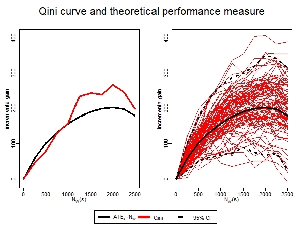
where is the average treatment effect of the share highest ranked individuals and is the number of treated individuals within this share. In section 3.3 and C, we describe the relationship between this theoretical performance measure and the calculation rule by Radcliffe 2007 in more detail. Figure 1 depicts a Qini curve calculated on a test set in relation to the theoretical performance measure. While the theoretical performance measures are intuitive, a practical challenge is that we do not observe in the test set. Hence, we cannot calculate and . Instead, the literature suggests ways to estimate and use these estimates in the above definitions of the performance measures (2) and (3). It is this estimation of where variance enters the evaluation metrics. Instead of getting performance values (2) or (3), the obtained evaluation metrics are only estimates for them. These estimates vary across observations in the test set and thus across test sets.
In the next two sections, we show how the evaluation metrics are calculated in practice. Thereby, we derive a simple mathematical expression for the variance in the evaluation metrics. Given this expression, it will be easy to see that current uplift model evaluation practices suffer from unnecessarily high variance and how the variance of the metrics can be reduced.
3.2 Transformed outcome mean squared error
The transformed outcome mean squared error is an approach to evaluate uplift models according to the mean squared error loss defined in equation (2). Gutierrez and Gérardy 2017 and Hitsch and Misra 2018 suggest to replace by the transformed outcome , where is the Horvitz-Thompson transformation, defined by
| (4) |
We denote the resulting transformed outcome mean squared error by
| (5) |
In previous literature, this metric is applied to evaluate model predictions on RCT data (Hitsch and Misra 2018; Haupt and Lessmann 2022). For observational data, the same metric could be applied with the only difference that the constant in needs to be replaced by a propensity score , estimating the treatment probability of each individual .
The causal inference literature suggests some alternative empirical evaluation metrics to estimate the theoretical accuracy performance (2) (Saito and Yasui 2020; Schuler and Shah 2018). However, in C.3, we show that except for the (and outcome adjusted versions of it), these metrics are biased on RCT data. Therefore, we restrict the following analysis to the .
Now, we analyze the expected value and variance of . For the expected value, it is useful to analyze the difference in between two uplift models because the expected value of the for a single model entails some hard-to-interpret expressions, which would make our discussion unnecessarily complex (Gutierrez and Gérardy 2017). In A.1, we derive that the expected value of the difference in between two models is given by
| (6) |
This result is reassuring as it shows that the evaluation is unbiased. In expectation, the difference in is the difference in the theoretical MSE from equation (2).
For infinite sample size, the empirical evaluation metric would exactly correspond to the theoretical performance in equation (6). However, as the (test) sample size is always finite in practice, we derive the variance of the difference in in A.1. Since this analysis is quite complex, we rather present only the essence of our analysis here. The important result is that the variance of the difference in depends on the variance of the transformed outcome and certain irreducible components. Using the law of total variance, the variance of the transformed outcome can be decomposed to
| (7) |
Any methods striving for a variance reduction of the thus need to reduce the two components on the right side of the above equation.
We close this section by providing some intuition about this result. The idea behind the is to replace the true CATE by an unbiased estimator - the transformed outcome . This transformed outcome varies around and this variance translates into the variance of the . So, it is intuitive that any potentially reducible variance in the is due to the variance of .
3.3 Qini curve
The Qini curve is an approach to empirically evaluate uplift models according to their ranking ability on the test set. Many slight variations of the Qini curve have appeared in the literature (Devriendt et al. 2020). There are also other names like "uplift curve", which basically refer to the same metric. In the following, we limit our analysis to the Qini curve suggested by Radcliffe 2007. Importantly, the results of our analysis can be transferred to other versions of the Qini curve, C discusses these other forms in more detail.
For his Qini curve, Radcliffe 2007 measures, for each share of highest ranked individuals, by how much the outcome increased due to the treatment. He calls this the "incremental gain", which he calculates by
where is the number of treated individuals within the share of the highest ranked individuals in the test set and is the number of untreated individuals within the share of the highest ranked individuals in the test set. and refer to the outcomes of the treated respectively untreated individuals. The Qini curve is then just a plot of for selected shares .
To see how this Qini curve relates to the theoretical performance measure of equation (3), we write down an empirical estimator of the average treatment effect for the share highest ranked individuals
| (8) |
We note that the qini curve can then be written as
So, the Qini curve calculated on the test set can be seen as an estimate for the theoretical ranking performance . The relationship between and the theoretical performance measure is illustrated in Figure 1.
Next, we discuss bias and variance of the Qini curve. For these statistical properties, the factor in the Qini curve is irrelevant. It is sufficient to examine the bias and variance of as an estimator for . From the definition of as the difference in sample means, it is clear that is unbiased (see A.2), that is
| (9) |
where belongs to the individuals in the highest ranked share . For the variance, we derive in A.2
where the outcome on the right side of the equation belongs to the share of the highest-ranked individuals. What is important here is that the metrics variance depends on . This is one of the two variance components of in equation (7), only with being the fraction of treated within the share , instead of the treatment probability in the RCT.
4 Metric variance reduction by outcome adjustment
4.1 The principle of variance reduction
In our analysis of the uplift evaluation metrics, we found that their variance depends on the variance of . Accordingly, it is worthwhile to analyze the variance of in detail and examine whether it could be reduced. For this purpose, it is useful to write in the following form
| (10) |
where is called the nuisance function in the following. Given this equation, we can easily explain the idea of variance reduction: The purpose of in the evaluation metrics is always to replace the unobservable . Everything except on the right side of equation (10) only causes variance of around , and this variance will enter the evaluation metrics. Hence, it would be ideal to remove and . However, is irreducible, because it is due to the unexplainable noise. But if we could remove , this would already lead to a reduction of variance. The idea behind outcome adjustment is simply to train a supervised learning model for the nuisance function on the training data and adjust the outcome to on the test data. Then, the reducible noise component becomes . In the following, we examine under which conditions such an outcome adjustment leads to a variance reduction of and thereby of the evaluation metrics.
First, we want to examine in more detail how the nuisance function affects the variance of the uplift evaluation metrics. Remember that the variance of can be decomposed into two components (see equation (7)). In B.1, we derive the following equations for these components
| (11) | ||||
| (12) |
These equations clearly show how the nuisance function affects the variance components of . In section 3.2, we have seen that both components determine the variance of the . In section 3.3, we have seen that only the first component affects the Qini curve. This leads to the following conditions for variance reduction of the evaluation metrics: If an adjustment function fulfills
| (C1) |
this leads to a variance reduction of the . If the adjustment function further fulfills
| (C2) |
this leads to further variance reduction of the and additionally reduces the variance of the Qini curve. The conditions (C1) and (C2) lead directly to plausible choices of adjustment functions .
4.2 Outcome adjustment methods
In this section, we provide adjustment methods that fulfill conditions (C1) and (C2) and thereby reduce the variance of the evaluation metrics. We start with condition (C1). This condition is already fulfilled if we construct a suitable estimate of . Using the outcome representation (1), we can verify that
So, an easy choice for an adjustment function would be the unconditional mean adjustment
| (AM1) |
where are respectively the sample averages of the treated and untreated in the training set. Note that the unconditional mean adjustment is constant in . This is why it has no effect on condition (C2). So, using this adjustment method, the variance of the Qini curve remains unaffected.
Next, we examine how an adjustment method could fulfill condition (C2). Again, we can use the outcome representation (1) to verify that
The conditional expected values on the right-hand side are the targets of supervised learning models for the outcome of the treated respectively untreated individuals. So, a natural choice for the adjustment function would be
| (AM2) |
where are supervised learning models trained on the treated respectively untreated individuals in the training set. We call this method doubly-robust adjustment because we can show that corresponds to the famous doubly robust outcome transformation (Robins and Rotnitzky 1995) adapted to RCT data (that means is a fixed value instead of a propensity score). It can be shown that the doubly-robust method Yadlowsky et al. 2021 apply to estimate the Qini curve on RCT data is equivalent to this doubly-robust outcome adjustment combined with the traditional way of Radcliffe 2007 to calculate the Qini curve. Furthermore, the doubly-robust version of the , which Saito and Yasui 2020 analyze on observational data is similar to , only with an estimated propensity score instead of a fixed probability . In the most common RCT case, where , another adjustment method is plausible. This is because in this case:
This makes conditional outcome adjustment a plausible method. The adjustment function is given by
| (AM3) |
with denoting a supervised learning model trained on the whole training data (treated and untreated individuals combined).
4.3 Practical impact of the adjustment methods
In the previous sections, we derived adjustment methods from theoretical results regarding the variance of uplift evaluation methods. Next, we analyze what is expected to happen if we apply them in practice. Specifically, we will deal with three questions: Can outcome adjustment bias uplift evaluation metrics? Does outcome adjustment always reduce the variance of an uplift evaluation metric or could it even increase variance? What is the practical impact of variance reduction?
We start with bias. Interestingly, the adjustment methods can not introduce bias in the evaluation metrics simply because the adjustment functions are fitted on the training set and not on the test set, where they are used for adjustment. On the test set, is just a fixed function. In consequence, the outcome in equation (1) becomes
with . In the equations (6) and (9) for the expected value of the and the Qini curve, the conditional expected value of the outcome does not appear. Accordingly, these expected values are unaffected by the shift in conditional expected value to . Hence, the metrics remain unbiased by outcome adjustment. We highlight that this only holds if the adjustment functions are not trained on the test set. The same principle of unbiasedness by doing model training and effect estimation on different data sets applies in previous literature about CATE model training under the name "cross fitting" (Chernozhukov et al. 2018) or "honest trees" (Wager and Athey 2018).
Next, we discuss whether outcome adjustment always leads to variance reduction. This equates to asking whether conditions (C1) and (C2) always hold for the suggested adjustment methods. In B.2, we provide a theoretical argument why it is almost impossible for the adjustment methods to fail condition (C1) unless is almost zero. Regarding condition (C2), we already noted that unconditional mean adjustment has no effect. For the doubly-robust and the conditional mean adjustment, we show that condition (C2) is fulfilled if their adjustment functions approximate better than a naive model (). So, if the underlying supervised learning models of the adjustment methods are not fitted very poorly, condition (C2) holds. In summary, if the training of the adjustment functions is done properly, there will, except for very special settings ( and ), be a reduction of the metrics variance. However, the magnitude of this effect is not yet clear.
Last, we discuss the impact of variance reduction. In practice, analysts have a test set on which they evaluate uplift model performance. On this test set, the variance of an evaluation metric would be reflected in the width of the confidence interval of an evaluation metric. Clearly, wide confidence intervals indicate that the model evaluation offers little certainty about the real (theoretical) performance of the model. In A.3, we derive formulas for confidence intervals of the and the Qini curve. From these formulas, an important fact can be derived: The width of the confidence interval is proportional to the square root of the variance of the error metrics and anti-proportional to the sample size of test set. This implies that reducing the variance of a metric by outcome adjustment allows for a reduction of the test set sample size without affecting the certainty of evaluation (width of confidence interval). Therefore, a reduction of variance by x% can be understood as a reduction of the required test set size by x%. In the following empirical analysis, we will measure the magnitude of this reduction.
5 Empirical analysis
In this section, we empirically assess the impact of the outcome adjustment methods. We provide the results of an experiment with simulated data as well as an experiment with three real-world data sets. The complete code for the empirical analysis is publicly available at (Bokelmann 2022).
5.1 Data
5.1.1 Simulated data
For two simulation settings, we made 10.000 simulation runs. In each of the 10.000 simulation runs, we generated 15.000 samples as a data set and used 10.000 observations for training and 5.000 observations for evaluation. We choose simulated data from two previously published studies using the R function "generate_causal_data" from the grf package (Tibshirani et al. 2022). Each of the settings simulates the features and the treatment group , as well as the outcome of the form
where . We always used 6 features . We choose three different values of the error standard deviation .
The two simulation settings are taken from, respectively, Wager and Athey 2018 and Nie and Wager 2021, and are denoted by "aw" and "nw" in the following. The simulation parameters for aw are
The "nw" simulation parameters are
5.2 Real-world data
For our real-world data analysis, we use three data sets: The publicly available Criteo data set provided by Diemert et al. 2021, the publicly available Hillstrom data set provided by Hillstrom 2008, and a data set related to digital couponing, which was provided by an online retailer (Haupt and Lessmann 2022; Gubela et al. 2020). We refer to the latter data set as "the private data set".
All of these data sets contain data of RCT’s. The Criteo data set contains 13,979,592 observations and one randomized treatment with a treatment probability of . The Hillstrom data set contains two different treatments (advertisement for women’s or men’s clothes), of which we deleted the observations with an advertisement for men’s clothes, to obtain an RCT with one treatment and a treatment probability of and 42,693 observations. The private data set contains 144,630 observations with one treatment and a treatment probability of .
From the Hillstrom and the private data set, we used 80% of the data for training and 20% of the data for testing. The Criteo data set, with its very large sample size, posed some computational challenges. From this data set, we used 90% of the observations for testing and the remaining observations for training.
5.3 Models for uplift and outcome adjustment
The actual choice of an uplift model to evaluate is of little importance for the empirical analysis. We do not want to find out which uplift modeling method is the best, but rather how to reliably evaluate an uplift model (no matter which). The only point to consider when choosing an uplift model was that the is only applicable to a model that yields CATE predictions. We choose a causal random forest for our analysis (Athey et al. 2019). Tuning parameters were fixed according to run time aspects: For the computationally intensive simulation, we fixed 1.000 trees and took the default parameters from the causal_forest-function (Tibshirani et al. 2022). For the large Criteo data set, we also fixed 1.000 trees and further reduced run time by fitting the model on a subset of size 100,000 from the training data. For the smaller private and the Hillstrom data, we increased the number of trees to 2.000.
To enable outcome adjustment, we also fit supervised learning models , and (see section 4.2) using the random forest implementation of the ranger package (Wright and Ziegler 2017).
5.4 Assessment criteria
We measure the impact of the outcome adjustment by comparing the ’s and the Qini curve’s variance when calculated based on the adjusted outcome with the variance when calculated based on the original outcome. On the simulated data, we calculated the variance between the evaluation on the 10.000 test sets. On the real-world data sets, this is not possible because we just have a limited number of observations. Therefore, we calculated confidence intervals for the evaluation metrics on each of the real-world data sets (see A.3 for details) and took the variance estimate of the confidence interval as an estimate of the metric’s variance.
For the Qini curve, this variance can be calculated for each share . On the real-world data sets, we calculated the variance at each decile (). On the simulation data, we only calculated the variance at the point , due to computational reasons. For the , we calculated differences
between the causal random forest and the trivial prediction . Because outcome adjustment changes the expected value of but does not affect the expected value of , comparing the variances of between adjusted and original outcome is more meaningful.
In addition to the variance reduction, we calculated a second evaluation quality measure: For the on the simulated data, we calculated the "share of misleading evaluations". Thereby, we considered an evaluation misleading if , although the theoretical performance of is better than the performance of . We calculated the share of misleading evaluations for comparisons of with the trivial predictions , the perfect predictions , and the original causal random forest with some added noise , where is the standard deviation in the predictions of . In fact, misleading predictions are a consequence of the variance of an evaluation metric. Hence, measuring a reduction of the variance already guarantees that the probability of misleading evaluations decreases. But we think it is worth considering the share of misleading evaluations in addition to the percentage of variance reduction because it allows for a better understanding of the impact of variance reduction.
5.5 Results
5.5.1 Variance reduction
Tables 1 and 2 show the percentage of variance reduction for the adjusted outcome-based metrics compared to the original outcome-based metrics. Notably, in each considered scenario (be it simulated data or real-world data) and for each metric, we observe a reduction in variance. This confirms our theoretical results.
For the , unconditional mean adjustment leads to a sizeable variance reduction but, as expected, the variance reduction of conditional mean adjustment and doubly-robust adjustment is stronger in each scenario. For the simulated data, the variance reduction by conditional mean adjustment and doubly-robust adjustment surpasses even 90% in some settings. For the real-world data, the reduction is smaller but still ranges between 12.4% to 34.1%. Likely, the gap between simulation settings and real-world data is due to the smaller impact of noise in the simulation. We can see that the variance reduction decreases with an increase in the noise standard deviation . Increasing from 2 to higher values would probably yield a variance reduction comparable in magnitude to what we observe in the real-world data settings.
For the Qini curve, we generally notice a smaller variance reduction. This is again in line with our theory. For the Qini curve, outcome adjustment only reduces the variance of component (11) but, in contrast to the , not of component (12). The variance reduction of the Qini curve is always stronger than 10% except for the Hillstrom data set, where the improvement is marginal. This shows that in real-world applications we would always expect to achieve a variance reduction but there is no guarantee that this reduction is sufficiently large to be practically relevant. The small improvement on the Hillstrom data set can be explained in the following way: On this data set, there is high treatment effect heterogeneity (variance in ), which is why it is possible to build useful uplift models on the data, but low hetorogeniety in the expected outcome (variance in ). As the variance in drives the reducible variance in the uplift metrics, there is little potential for improvement.
In summary, conditional mean and doubly-robust adjustment reliably lead to a variance reduction of the and the Qini curve. The practical implications are easy to see when we translate the variance reduction into a reduction of the required test set sample size. For example, on the Criteo data set, applicants could save more than 10% of the test set data and still benefit from the same confidence in their model evaluations if they apply outcome adjustment. As RCT data is costly to obtain, a substantial reduction of the required (test) sample size has practical relevance.
The results of tables 1 and 2 already provide clear evidence in favor of the use of outcome adjustment. However, we think that to better understand the rather abstract concept of variance reduction, some visualizations are helpful. Hence, we close this section by referring to Figures 2, 3 and 4, which illustrate the results from table 1 and 2. The figures demonstrate the effect of outcome adjustment from a different perspective. For example, 4 shows the Qini curve calculated on the private data set by the original outcome and the adjusted outcomes. It demonstrates how variance reduction translates into smaller confidence intervals and additionally provides the variance reduction at each decile. Plots of the Qini curve for the other real-world data sets as well as plots of the distribution of are provided by Bokelmann 2022.
| Setting | Qini0.1(cond) | Qini0.1(dr) | ||||
|---|---|---|---|---|---|---|
| ’aw’ | 0.5 | 89.7% | 97.8% | 97.8% | 10.1% | 11.7% |
| ’aw’ | 1 | 83.0% | 91.3% | 91.4% | 30.6% | 31.3% |
| ’aw’ | 2 | 62.9% | 69.8% | 70.0% | 14.3% | 15.1% |
| ’nw’ | 0.5 | 60.3% | 94.4% | 93.8% | 71.9% | 69.5% |
| ’nw’ | 1 | 51.6% | 80.8% | 80.6% | 47.5% | 46.9% |
| ’nw’ | 2 | 28.4% | 44.4% | 45.0% | 17.0% | 17.8% |
-
The table shows the percentage of variance reduction of the adjustment methods compared to the original outcome. The difference in was calculated between and . For the Qini curve, the table shows the variance reduction at point .
| data | Qini(cond) | Qini(dr) | |||
|---|---|---|---|---|---|
| private | 16.4% | 34.1% | 33.3% | 15.6-25.1% | 15.1%-23.8% |
| Criteo | 0.4% | 13.8% | 12.4% | 12.7-13.7% | 11.3-12.1% |
| Hillstrom | 14.4% | 16.7% | 16.6% | 1.79-3.30% | 1.75-3.19% |
-
The table shows the percentage of variance reduction of the adjustment methods compared to the original outcome. The difference in was calculated between and . For the Qini curve, the table shows highest and lowest variance reduction over the 10 deciles, the Qini curve was claculated on.
5.5.2 Reduction of misleading evaluations
Table 3, shows the share of misleading evaluations by on the simulated data. In some scenarios, the results are quite remarkable: For "aw" with , the based on the original outcome mistakenly judges to perform better than the perfect prediction in 39.3% of the cases. The conditional mean or doubly-robust outcome adjustment reduces this share of misleading evaluations to 4.5% and 4.4%, respectively. On one hand, this demonstrates the high degree of randomness in model evaluations if the test set is not large enough. On the other hand, the result also displays the big impact that outcome adjustment can have on the quality of evaluations. Overall, the share of misleading evaluations is reduced by any of the adjustment methods in any setting. Thereby, as expected, conditional mean adjustment and doubly-robust adjustment perform better than unconditional mean adjustment.
| Setting | orig | cond | uncond | dr | ||
|---|---|---|---|---|---|---|
| "aw" | 39.3 | 4.5 | 23.6 | 4.4 | ||
| "aw" | 32.9 | 9.0 | 17.3 | 8.7 | ||
| "aw" | 25.1 | 9.4 | 11.2 | 9.2 | ||
| "aw" | 6.1 | 0.0 | 0.0 | 0.0 | ||
| "aw" | 7.6 | 0.0 | 0.0 | 0.0 | ||
| "aw" | 9.9 | 0.7 | 1.3 | 0.7 | ||
| "aw" | 48.6 | 39.0 | 44.7 | 38.8 | ||
| "aw" | 47.7 | 43.6 | 45.4 | 43.4 | ||
| "aw" | 48.5 | 46.4 | 46.6 | 46.4 | ||
| "nw" | 33.8 | 5.6 | 26.1 | 6.6 | ||
| "nw" | 26.4 | 8.0 | 19.6 | 8.2 | ||
| "nw" | 15.9 | 10.7 | 13.0 | 10.7 | ||
| "nw" | 16.8 | 0.0 | 7.0 | 0.0 | ||
| "nw" | 28.5 | 11.9 | 20.8 | 11.8 | ||
| "nw" | 56.9 | 40.8 | 41.7 | 40.8 | ||
| "nw" | 46.3 | 38.8 | 44.7 | 38.9 | ||
| "nw" | 46.7 | 43.8 | 44.8 | 43.7 | ||
| "nw" | 45.6 | 44.4 | 44.9 | 44.2 |
-
The table shows the percentage of misleading evaluations, that is the share of simulation runs, where the MSE for was lower than the MSE for , higher then for or higher than for .
6 Conclusion
In this paper, we showed that the statistical properties of the uplift evaluation metrics depend on the variance of the transformed outcome . We also demonstrated that the variance of the transformed outcome can be reduced by fitting appropriate models on the training set and adjusting the outcome on the test set to . Importantly, our analysis confirmed that a corresponding adjustment leaves evaluation metrics unbiased and only reduces their variance. This reduced variance leads to a more reliable evaluation of uplift models according to the and also according to the Qini curve. For example, we found that an outcome adjustment produces far fewer misleading model comparisons by the .
We described three possible outcome adjustment techniques, which we derived from the theoretical analysis. The unconditional mean adjustment leads to a reduction of variance for the , but leaves the Qini curve unaffected. The conditional mean adjustment and the doubly-robust adjustment reduce the variance of the as well as the Qini curve. In all considered empirical settings, the conditional mean adjustment and the doubly-robust adjustment reduced the variance of the metrics more than the unconditional outcome adjustment.
For practical applications, we suggest to never use the with the original outcome. The results of our empirical analysis indicate that conclusions based on the with the original outcome could be severely misleading. Further, our theoretical analysis and empirical results clearly show that it is generally better to use adjusted outcomes. The easiest adjustment method is the unconditional mean adjustment because it does not require fitting a supervised learning model. But as we have seen, it is also inferior to the alternative adjustment approaches in form of the conditional mean adjustment or doubly-robust adjustment.
Practical consequences of the variance reduction can be seen in two ways: If applicants evaluate uplift models on a given test set, evaluations based on the adjusted outcomes are more reliable than evaluations based on the original outcomes. Applicants would benefit from smaller confidence intervals due to our adjustments. Another benefit concerns the sample sizes needed to achieve a certain level of reliability (width of confidence interval). We have shown that variance reduction can translate into a reduction of the required sample size. Our empirical analysis shows that a reduction of the required test sample size of 10% and more are realistic in practice.
In this paper, we focused on the and the Qini curve as empirical uplift evaluation metrics. In the Appendix, we also summarised the other metrics, which appear in the uplift literature. We theoretically show that the principle of variance reduction by outcome adjustment also applies there. In fact, we are not aware of a form of uplift model evaluation that would not benefit from outcome adjustment. However, the magnitude of improvement depends on the specific data set and may be small.
In summary, the suggested outcome adjustment methods offer clear practical benefits in terms of variance reduction. They also do not bring notable disadvantages: they are easy to apply, can not cause bias, and will almost surely reduce variance unless the required supervised learning models predict worse than a naive model. For these reasons, we think it is worth changing current state-of-art uplift evaluation procedures towards using adjusted outcomes.
Appendix A Derivation of the metric distributions
A.1 Derivation of the transformed mean squared error distribution
Given the outcome representation in equation (1), we can write the transformed outcome as
with . The difference in squared deviation from between two estimators then becomes
Using the fact that and are functions in , we can see that
In this way, we can derive equations for the expected value and variance of the . We denote the difference in by . Note that the is an average of squared deviations of the estimators from . The above equations then become
| (13) | ||||
| (14) |
Equation (13) shows that is unbiased. Now, we examine the variance. Given the law of total variance, we obtain
From equation (13), we see that the second term does not depend on the outcome and is hence not reducible. Accordingly, the reducible part of the variance is
Some transformations yield
Minimizing this irrespective of the choice of and , which is a plausible approach as the metric should be optimal for the evaluation of all estimators, corresponds to minimizing . To do this, we again apply the law of total variance
So, in summary, a reduction of corresponds to a reduction of .

A.2 Derivation of the Qini metric distribution
The estimate of the average treatment effect for the share of highest ranked individuals is
where the outcomes belong to individuals ranked in the highest share and , denote the amount of treated and untreated individuals within this share, respectively. This expression can be transformed into
where and .
This estimate is unbiased:
where the CATE belongs to individuals ranked in the highest share . Next, we analyze the variance. By the law of total variance, we can derive
In this derivation, follows from the definition of , which makes constant irrespective of . Thus, the variance of is
where we keep in mind that the outcome on the right side of the equation belongs to individuals in the share with the highest rank.

A.3 Calculation of confidence intervals
The distribution of an evaluation metric determines the confidence intervals. For unbiased error metrics like the and the Qini curve, the variance translates into the width of the confidence interval. Next, we derive formulas for the confidence intervals of the and the Qini curve.
For the Qini curve, we can construct a confidence interval at each point by analyzing the distribution of around the theoretical value . Given equation (8) for the original outcome, we can assume asymptotic normality with
where the outcome belongs to the share of highest ranked individuals. As the values of the Qini curve are calculated as , the 95% confidence interval at each point can be constructed by
where are the empirical estimates for and and is the total number of individuals within the share with highest rank. In the same way, we can calculate confidence intervals for the adjusted outcomes.
For the , it is of little use to compare confidence intervals between the original and the adjusted outcomes because outcome adjustment changes the expected value of . Confidence intervals for the different outcome versions would thus be built around different parameters. Instead, it is plausible to calculate confidence intervals for a difference in because for differences, outcome adjustment does not change the expected value. The difference in can be written as
As a mean of independent summands, is asymptotically normally distributed. Hence, a confidence interval can be calculated by
where is the empirical standard deviation between the summands .

Appendix B Variance components of the transformed outcome
B.1 Calculation of the variance components
In section 4, A.1, and A.2, we have examined the variance of the uplift evaluation metrics and have found that the variance of the depends on both of the components and . We have further found that the variance of the Qini curve only depends on the first of these components, with the slight modification that the treatment probability in the RCT needs to be replaced by the fraction of treated within the share of highest ranked individuals.
Here, we further decompose the variance components to reveal their relationship to the nuisance function . It holds
To reduce the variance of the transformed outcome, we need to reduce and . Note that the latter term only affects the transformed outcome for the MSE, while the former affects also the transformed outcome for the rank metrics.
B.2 Reduction of the variance components
In this section, we show that a supervised learning model for the target will generally fulfill conditions (C1) and (C2) for variance reduction. We start with condition (C1). The mean squared error, which is the plausible optimization criterion for , can be written as
Assume condition (C1) is not fulfilled. Then the difference in expected values, in the second component, would be larger than in expected value. In case the difference in expected values is positive and we shift our model by a constant , the second component would be reduced. In case the difference in expected values is negative and we choose , the second component would again be reduced. Such a constant shift of the model would not affect the first component on the right-hand side. Accordingly, such a shift would reduce the MSE. For a properly fitted model, it is impossible to miss such a simple shift during the training unless is close to zero. So, if is not close to zero, condition (C1) will be fulfilled. We next examine condition (C2). If is an estimator for that is more precise than the trivial in terms of the MSE loss, then
So, any supervised learning model for the parameter that predicts better than a naive model will fulfill condition (C2) for variance reduction.
Appendix C Other evaluation metrics
In our analysis of error metrics, we have focused on the Qini curve and the , which are commonly used in the uplift literature. Here, we summarise other evaluation metrics found in the literature and show that our results also apply to these metrics. In general, there are three classes of empirical evaluation metrics: rank metrics, treatment decision metrics, which measure the impact of allocating treatment according to the uplift model, and accuracy metrics. The Qini curve belongs to the first class and the to the third. In the following, we will examine other members of these three metric classes.
C.1 Rank metrics: Qini curve, uplift curve, and related measures
In section 3.3, we analyzed the Qini curve by Radcliffe 2007, as one of the most popular empirical ranking evaluation methods. This curve is given by
| (Q1) |
where and denote the number of treated respectively untreated in the share of highest ranked individuals. Note that here we use in the notation and not to highlight that we only count the number of treated within the share and not in the whole data set. This is important to represent differences to other variants of the Qini curve. Devriendt et al. 2020 provide an extensive review of alternative approaches to calculate the Qini curve. In the following, we briefly examine these variants and show why our statistical analysis for the original Qini curve also applies.
The first variation of the Qini curve is, for example, used by Diemert et al. 2021. They calculate the Qini curve as
| (Q2) |
Another version of the Qini curve is provided, for example, by Guelman 2015, where it is defined by
| (Q3) |
These alternative Qini curves fit our analysis of the statistical properties of the original Qini curve. For (Q1), it holds . For (Q2), it holds due to the random treatment allocation and . This leads to . For (Q3), it holds for similar reasons . So, all the Qini curve versions correspond to multiplied by a factor that is unrelated to the distribution of the outcome. This is exactly the same situation as for the original Qini curve. In the analysis of its statistical properties, we only needed to examine the properties of . And as we can see, these also determine the statistical properties of the other Qini curve versions.
One "alternative" to the Qini curve is the so-called "uplift curve". In some studies like Gutierrez and Gérardy 2017, the uplift curve is given by
| (UC1) |
In other papers, like Jaskowski and Jaroszewicz 2012, it is given by
| (UC2) |
Another alternative is provided by Kuusisto et al. 2014, who calculate the uplift curve by
| (UC3) |
Again, these forms of the uplift curve fit our analysis of the statistical properties of the original Qini curve. For (UC1), we can see that . For (UC2), we can see that due to random treatment allocation and . This then leads to . As to (UC3), this metric only works of the treatment property if . Then, and, therefore, . So, with the same argumentation as for the alternative Qini curves, we can see that the statistical analysis of the original Qini curve applies to different forms of uplift curves.
Another related way to empirically evaluate the ranking of a model is to visualize the "uplift per decile", as done by Kane et al. 2014. This works by estimating the average treatment effects per decile as the difference in mean outcomes between the treated and untreated. Statistically, this is the same as what happens in equation (3), just that the outcomes belong to individuals whose predictions are in a certain decile instead of the share of individuals with the highest rank. Therefore, we can also transfer the statistical analysis to this evaluation metric.
In addition to the various versions of Qini and uplift curves, some evaluation measures are derived from these curves. An example is the area under the uplift curve (AUUC), which Devriendt et al. 2020 calculate as
Of course, the statistical properties of this measure depend on the statistical properties of the uplift curve . Since the statistical properties of the uplift curve can be analyzed in the same way as the statistical properties of the Qini curve by Radcliffe 2007, the results of our statistical analysis directly transfer to the area under the uplift curve.
Finally, Radcliffe 2007 defines two Qini values, which he derives from the Qini curve. The Qini values measure two versions of a ratio between the Qini curve and a theoretical optimum. Again, our statistical analysis holds for these measures because it concerns the statistical properties of the Qini curve.
In summary, we find out statistical analysis holds for a range of ranking evaluation measures used in the uplift modeling literature and different versions of these measures. This also implies that all of these measures and versions suffer from variance and will benefit from the proposed adjustments for variance reduction.
C.2 Treatment decision metrics
Instead of measuring how well a model ranks individuals according to , it is also possible to measure what happens if we derive concrete treatment allocation decisions from an uplift model. There are two theoretical parameters that would measure model performance: The gain and the expected outcome if treatment allocation works according to the model decisions.
The gain could be estimated by
where the outcomes belong to individuals for which the model recommends treatment (Schuler and Shah 2018). This is again an average treatment effect estimator by differences in the means between the treated and the untreated. So, just like in the analysis of the Qini curve Radcliffe 2007, our results concerning variance reduction apply.
The expected outcome if treatment is assigned according to uplift model recommendation can be estimated by
where . This metric appears in the literature under the name "decision value" (Schuler and Shah 2018; Kapelner et al. 2014; Zhao et al. 2017). Hitsch and Misra 2018 use the same metric under the name "targeting profit", the only difference being that they added a cost for each decision to treat, which is irrelevant in terms of the statistical properties. is more challenging to discuss than any of the other empirical evaluation metrics described so far. This is because outcome adjustment would bias the metric (because of ). But if we use this metric to evaluate which of two decision models yields better decisions, the bias due to outcome adjustment disappears because
To derive that the variance can be reduced, we write the difference between the empirical estimates as
We obtain sums of transformed outcomes in this expression. In section 4, we have shown that outcome adjustment leads to a reduction of . This would then also apply for the difference .
C.3 Accuracy metrics
Here, we discuss alternative accuracy metrics beyond the . The first two methods are described and evaluated by Saito and Yasui 2020 in the context of observational data. Here, we discuss them in the context of RCT data. The first method is the plug-in evaluation. It measures the uplift model performance by
where and are estimators of the conditional expected value of the treated and untreated respectively. In an empirical analysis, Saito and Yasui 2020 found the slightly inferior to the with doubly-robust adjustment. In our opinion, however, there is a more serious problem with the . It is easy to verify that is biased. If we choose as a CATE estimator to evaluate, would be zero.
The second metric described and evaluated by Saito and Yasui 2020 is called -risk. It is based on the loss function of the R-learner from Nie and Wager 2021. For RCT data, where the treatment probability is constant, it would be defined as
where is an estimator of the conditional expected value of treated and untreated combined. In the empirical analysis by Saito and Yasui 2020, this metric does not perform well. Furthermore, just like the , this metric is also biased. We show this by using representation (1) of the outcome in the definition of the metric:
The expected value is given by . So, for an estimator with , the term is zero. Accordingly, this estimator would be preferred by the , compared to an estimator with the same theoretical performance , but with .
Another metric is the -loss described by Schuler and Shah 2018. It is only applicable to uplift models that yield, for each individual, two outcome predictions: if the individual is treated and if the individual is not treated. The -loss is then calculated by
In summary, accuracy evaluation metrics other than the are either biased or not generally applicable for CATE model evaluation. In our opinion, this renders the corresponding metrics unsuitable for the evaluation of uplift models on RCT data. Notably, bias disqualifies the metrics mainly for application to RCT. For observational data, any metric could be biased due to the unknown treatment probability . In contrast, on RCT data it is easy to build useful and unbiased evaluation metrics. Hence, any biased metric can be considered unsuitable. Accordingly, we would recommend to use the (with our suggested outcome adjustment methods) to evaluate the accuracy of uplift model predictions on RCT data.
References
- van Klaveren et al. [2018] David van Klaveren, Ewout W Steyerberg, Patrick W Serruys, and David M Kent. The proposed ‘concordance-statistic for benefit’provided a useful metric when modeling heterogeneous treatment effects. Journal of clinical epidemiology, 94:59–68, 2018.
- Haupt and Lessmann [2022] Johannes Haupt and Stefan Lessmann. Targeting customers under response-dependent costs. European Journal of Operational Research, 297(1):369–379, 2022.
- Lemmens and Gupta [2020] Aurélie Lemmens and Sunil Gupta. Managing churn to maximize profits. Marketing Science, 39(5):956–973, 2020.
- Devriendt et al. [2021] Floris Devriendt, Jeroen Berrevoets, and Wouter Verbeke. Why you should stop predicting customer churn and start using uplift models. Information Sciences, 548:497–515, 2021.
- Olaya et al. [2020] Diego Olaya, Jonathan Vásquez, Sebastián Maldonado, Jaime Miranda, and Wouter Verbeke. Uplift modeling for preventing student dropout in higher education. Decision Support Systems, 134:113320, 2020.
- Athey and Wager [2021] Susan Athey and Stefan Wager. Policy learning with observational data. Econometrica, 89(1):133–161, 2021.
- Cousineau et al. [2023] Martin Cousineau, Vedat Verter, Susan A. Murphy, and Joelle Pineau. Estimating causal effects with optimization-based methods: A review and empirical comparison. European Journal of Operational Research, 304(2):367–380, 2023.
- Gutierrez and Gérardy [2017] Pierre Gutierrez and Jean-Yves Gérardy. Causal inference and uplift modelling: A review of the literature. In International conference on predictive applications and APIs, pages 1–13. PMLR, 2017.
- Li et al. [2021] Jiuyong Li, Weijia Zhang, Lin Liu, Kui Yu, Thuc Duy Le, and Jixue Liu. A general framework for causal classification. International Journal of Data Science and Analytics, 11(2):127–139, 2021.
- Verbeke et al. [2023] Wouter Verbeke, Diego Olaya, Marie-Anne Guerry, and Jente Van Belle. To do or not to do? Cost-sensitive causal classification with individual treatment effect estimates. European Journal of Operational Research, pages 838–852, 2023.
- Devriendt et al. [2020] Floris Devriendt, Jente Van Belle, Tias Guns, and Wouter Verbeke. Learning to rank for uplift modeling. IEEE, 2020.
- Devriendt et al. [2018] Floris Devriendt, Darie Moldovan, and Wouter Verbeke. A literature survey and experimental evaluation of the state-of-the-art in uplift modeling: A stepping stone toward the development of prescriptive analytics. Big data, 6(1):13–41, 2018.
- Gubela et al. [2020] Robin M Gubela, Stefan Lessmann, and Szymon Jaroszewicz. Response transformation and profit decomposition for revenue uplift modeling. European Journal of Operational Research, 283(2):647–661, 2020.
- Fernández-Loría and Provost [2022] Carlos Fernández-Loría and Foster Provost. Causal classification: Treatment effect estimation vs. outcome prediction. Journal of Machine Learning Research, 23(59):1–35, 2022.
- Schuler and Shah [2018] Alejandro Schuler and Nigam Shah. General-purpose validation and model selection when estimating individual treatment effects. arXiv preprint arXiv:1804.05146, 2018.
- Saito and Yasui [2020] Yuta Saito and Shota Yasui. Counterfactual cross-validation: Stable model selection procedure for causal inference models. In International Conference on Machine Learning, pages 8398–8407. PMLR, 2020.
- Zhao et al. [2017] Yan Zhao, Xiao Fang, and David Simchi-Levi. Uplift modeling with multiple treatments and general response types. In Proceedings of the 2017 SIAM International Conference on Data Mining, pages 588–596. SIAM, 2017.
- Haupt et al. [2019] Johannes Haupt, Daniel Jacob, Robin M Gubela, and Stefan Lessmann. Affordable uplift: Supervised randomization in controlled experiments, 2019. URL https://arxiv.org/abs/1910.00393.
- Berrevoets et al. [2022] Jeroen Berrevoets, Sam Verboven, and Wouter Verbeke. Treatment effect optimisation in dynamic environments. Journal of Causal Inference, 10(1):106–122, 2022.
- De Caigny et al. [2021] Arno De Caigny, Kristof Coussement, Wouter Verbeke, Khaoula Idbenjra, and Minh Phan. Uplift modeling and its implications for b2b customer churn prediction: A segmentation-based modeling approach. Industrial Marketing Management, 99:28–39, 2021.
- Baier and Stöcker [2022] Daniel Baier and Björn Stöcker. Profit uplift modeling for direct marketing campaigns: approaches and applications for online shops. Journal of Business Economics, 92(4):645–673, 2022.
- Betlei et al. [2021] Artem Betlei, Eustache Diemert, and Massih-Reza Amini. Uplift modeling with generalization guarantees. In Proceedings of the 27th ACM SIGKDD Conference on Knowledge Discovery & Data Mining, pages 55–65, 2021.
- Hitsch and Misra [2018] Günter J Hitsch and Sanjog Misra. Heterogeneous treatment effects and optimal targeting policy evaluation. Available at SSRN 3111957, 2018.
- Bokelmann [2022] Björn Bokelmann. Code for the research paper, 2022. URL https://github.com/bokelmab/uplift_metrics.
- Jacob [2021] Daniel Jacob. Cate meets ml. Digital Finance, 3(2):99–148, 2021.
- Robins and Rotnitzky [1995] James M Robins and Andrea Rotnitzky. Semiparametric efficiency in multivariate regression models with missing data. Journal of the American Statistical Association, 90(429):122–129, 1995.
- Chernozhukov et al. [2018] Victor Chernozhukov, Denis Chetverikov, Mert Demirer, Esther Duflo, Christian Hansen, Whitney Newey, and James Robins. Double/debiased machine learning for treatment and structural parameters. The Econometrics Journal, pages 1–68, 2018.
- Saito [2020] Yuta Saito. Doubly robust estimator for ranking metrics with post-click conversions. In Fourteenth ACM Conference on Recommender Systems, pages 92–100, 2020.
- Wager et al. [2016] Stefan Wager, Wenfei Du, Jonathan Taylor, and Robert J Tibshirani. High-dimensional regression adjustments in randomized experiments. Proceedings of the National Academy of Sciences, 113(45):12673–12678, 2016.
- Guo et al. [2021] Yongyi Guo, Dominic Coey, Mikael Konutgan, Wenting Li, Chris Schoener, and Matt Goldman. Machine learning for variance reduction in online experiments. Advances in Neural Information Processing Systems, 34:8637–8648, 2021.
- Jin and Ba [2022] Ying Jin and Shan Ba. Towards optimal variance reduction in online controlled experiments. Technometrics, (just-accepted):1–33, 2022.
- Radcliffe [2007] Nicholas Radcliffe. Using control groups to target on predicted lift: Building and assessing uplift model. Direct Marketing Analytics Journal, pages 14–21, 2007.
- Saito et al. [2019] Yuta Saito, Hayato Sakata, and Kazuhide Nakata. Doubly robust prediction and evaluation methods improve uplift modeling for observational data. In Proceedings of the 2019 SIAM International Conference on Data Mining, pages 468–476. SIAM, 2019.
- Yadlowsky et al. [2021] Steve Yadlowsky, Scott Fleming, Nigam Shah, Emma Brunskill, and Stefan Wager. Evaluating treatment prioritization rules via rank-weighted average treatment effects. arXiv preprint arXiv:2111.07966, 2021.
- Alaa and Van Der Schaar [2019] Ahmed Alaa and Mihaela Van Der Schaar. Validating causal inference models via influence functions. In International Conference on Machine Learning, pages 191–201. PMLR, 2019.
- Mahajan et al. [2022] Divyat Mahajan, Ioannis Mitliagkas, Brady Neal, and Vasilis Syrgkanis. Empirical analysis of model selection for heterogenous causal effect estimation. arXiv preprint arXiv:2211.01939, 2022.
- Wager and Athey [2018] Stefan Wager and Susan Athey. Estimation and inference of heterogeneous treatment effects using random forests. Journal of the American Statistical Association, 113(523):1228–1242, 2018.
- Tibshirani et al. [2022] Julie Tibshirani, Susan Athey, Erik Sverdrup, and Stefan Wager. grf: Generalized Random Forests, 2022. URL https://CRAN.R-project.org/package=grf. R package version 2.1.0.
- Nie and Wager [2021] Xinkun Nie and Stefan Wager. Quasi-oracle estimation of heterogeneous treatment effects. Biometrika, 108(2):299–319, 2021.
- Diemert et al. [2021] Eustache Diemert, Artem Betlei, Christophe Renaudin, Massih-Reza Amini, Théophane Gregoir, and Thibaud Rahier. A large scale benchmark for individual treatment effect prediction and uplift modeling. arXiv preprint arXiv:2111.10106, 2021.
- Hillstrom [2008] Kevin Hillstrom. Minethatdata e-mail analytics and data mining challenge, 2008. URL https://blog.minethatdata.com/2008/03/minethatdata-e-mail-analytics-and-data.html.
- Athey et al. [2019] Susan Athey, Julie Tibshirani, and Stefan Wager. Generalized random forests. The Annals of Statistics, 47(2):1148–1178, 2019.
- Wright and Ziegler [2017] Marvin N. Wright and Andreas Ziegler. ranger: A fast implementation of random forests for high dimensional data in C++ and R. Journal of Statistical Software, 77(1):1–17, 2017. doi:10.18637/jss.v077.i01.
- Guelman [2015] Leo Guelman. Optimal personalized treatment learning models with insurance applications. Universitat de Barcelona, 2015.
- Jaskowski and Jaroszewicz [2012] Maciej Jaskowski and Szymon Jaroszewicz. Uplift modeling for clinical trial data. In ICML Workshop on Clinical Data Analysis, pages 79–95, 2012.
- Kuusisto et al. [2014] Finn Kuusisto, Vitor Santos Costa, Houssam Nassif, Elizabeth Burnside, David Page, and Jude Shavlik. Support vector machines for differential prediction. In Joint European Conference on Machine Learning and Knowledge Discovery in Databases, pages 50–65. Springer, 2014.
- Kane et al. [2014] Kathleen Kane, Victor SY Lo, and Jane Zheng. Mining for the truly responsive customers and prospects using true-lift modeling: Comparison of new and existing methods. Journal of Marketing Analytics, 2(4):218–238, 2014.
- Kapelner et al. [2014] A Kapelner, J Bleich, A Levine, ZD Cohen, RJ DeRubeis, and R Berk. Inference for the effectiveness of personalized medicine with software. arXiv preprint arXiv:1404.7844, 2014.