Supervised Metric Learning to Rank for Retrieval via
Contextual Similarity Optimization
Abstract
There is extensive interest in metric learning methods for image retrieval. Many metric learning loss functions focus on learning a correct ranking of training samples, but strongly overfit semantically inconsistent labels and require a large amount of data. To address these shortcomings, we propose a new metric learning method, called contextual loss, which optimizes contextual similarity in addition to cosine similarity. Our contextual loss implicitly enforces semantic consistency among neighbors while converging to the correct ranking. We empirically show that the proposed loss is more robust to label noise, and is less prone to overfitting even when a large portion of train data is withheld. Extensive experiments demonstrate that our method achieves a new state-of-the-art across four image retrieval benchmarks and multiple different evaluation settings. Code is available at: https://github.com/Chris210634/metric-learning-using-contextual-similarity
Keywords:
Machine Learning, ICML1 Introduction
Image retrieval refers to learning a ranking of instances from a gallery set relative to a query image such that the highest ranked instances are the most relevant to the query. Several real-world applications are powered by this technology, such as person re-identification (Ye et al. 2021), face recognition (Guillaumin et al. 2009), vehicle re-identification (Chu et al. 2019), landmark retrieval (Weyand et al. 2020), and product retrieval (Cakir et al. 2019). Current metric learning techniques often use a dataset with single discrete labels for supervision, and train an embedding space where images with the same label are closer together than images with different labels. However, binary supervision is unreliable, since it does not capture the complexity of relationships in the data. Furthermore, methods which overly rely on the binary supervision can be brittle in the presence of noise, since the supervision is either correct or incorrect. Multi-label datasets (Ranjan et al. 2015) mitigate this problem, but can be expensive to procure, so developing a metric learning method that is robust to label noise and generalizable to test data is a challenging yet important problem.
Existing image retrieval approaches fall into two main categories: classification and pairwise ranking losses. Classification losses optimize a classifier on top of the embedding layer and discard the classifier at the end of training. Pairwise ranking losses train the embedding layer directly by pulling together pairs of samples with the same label and pushing apart pairs of samples with different labels. Pairwise ranking methods include losses which explicitly optimize a ranking metric such as AP (average precision) surrogates: Fast-AP (Cakir et al. 2019), Smooth-AP (Brown et al. 2020), Blackbox AP (Rolínek et al. 2020) and Roadmap (Ramzi et al. 2021). They also include the standard contrastive, triplet and multi-similarity (MS) losses (Wang et al. 2019).

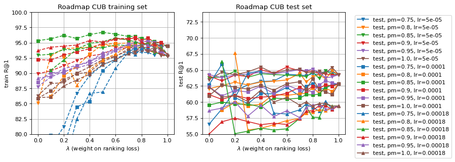
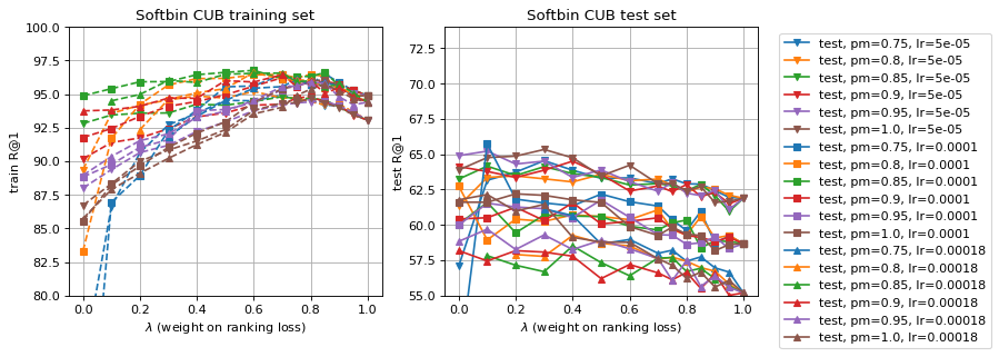
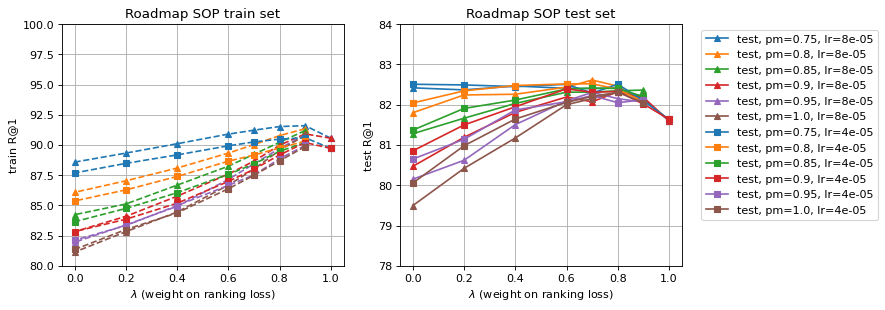
Empirically, classification methods, such as proxy anchor (Kim et al. 2020), proxy NCA (Teh et al. 2020), and HIST (Lim et al. 2022) perform well on small benchmark datasets, while multi-similarity and AP surrogates perform well on large datasets. This general trend is supported by our main results in Section 5. We hypothesize that pairwise ranking methods tend to overfit the training labels while sacrificing semantic consistency of the embedding space. This can be possible even if the labels are “correct”, as Figure 1 illustrates. For instance, pulling apart samples of white-necked ravens from common ravens would likely lead to overfitting, since the distinguishing visual attribute is absent from the images. To address this issue, we propose to optimize contextual similarity in addition to cosine similarity. The resulting loss function implicitly regularizes the embedding space for semantic consistency among neighbors (see results in Section 4). Figure 2 clearly shows that our method reduces overfitting, since we achieve the best test R@1 accuracy despite lower train R@1 accuracy than some baselines. Results in Section 5 show that our method outperforms all baselines across all standard benchmarks in terms of R@1 accuracy.

Contextual similarity is a widely used evaluation-time technique to boost retrieval accuracy. In simple terms, the contextual similarity is the fraction of neighbors two samples have in common in embedding space. Intuitively, two samples are more likely to share the same label if they have many neighbors in common, regardless of their cosine similarity. Many retrieval frameworks (Zhong et al. 2017, Cao et al. 2020) use a combination of cosine similarity and contextual similarity for evaluation, but only explicitly optimize the cosine similarity when training. In this paper, we propose to explicitly optimize both similarities, since contextual similarity captures crucial semantic information. In another line of work, some unsupervised metric learning methods such as STML (Kim et al. 2022) use contextual similarity to estimate the true similarity between unlabeled samples. Inspired by STML, we show that optimizing contextual similarity directly in the supervised setting is beneficial. As far as we know, we are the first to treat contextual similarity as a loss function for supervised learning. This is non-trivial since contextual similarity involves non-differentiable counting operations, and as a consequence, is not amenable to off-the-shelf optimization techniques. We propose a simple but effective optimization strategy in Section 3, using heuristic gradients. We analytically justify this optimization approach in Section 4.1.
Our contributions are as follows:
- 1.
We introduce the contextual loss, which establishes a new state-of-the-art across all standard image retrieval benchmarks, even when compared to more complicated (e.g. Metrix, HIST and AVSL) and less scalable methods (AP surrogates).
- 2.
Our contextual loss mitigates overfitting by implicitly enforcing semantic consistency among neighbors in the embedding space. As a result, we achieve a 4% improvement in R@1 accuracy over baselines in the presence of label noise.
- 3.
We conduct an extensive experimental study of our method and several popular baselines. This includes empirical results across five different benchmarks, two different experimental settings, accompanied by a comprehensive ablation study. In addition, we tune baselines extensively to promote fair comparisons.
- 4.
The optimization of non-differentiable steps in the loss calculation may be of interest to some readers.
This paper is organized as follows. Section 2 summarizes related work. Section 3 states our method, including how we optimize the non-differentiable steps in calculating contextual similarity. Section 4.1 checks that minimizing the contextual loss corresponds to learning the correct ranking of samples and that the proposed optimization procedure converges. The rest of Section 4 explores why the proposed contextual loss is less prone to overfitting than other pairwise ranking losses by analyzing gradients and running targeted experiments. Section 5 and the Appendix present an extensive experimental study. Code is available at: https://github.com/Chris210634/metric-learning-using-contextual-similarity
2 Related Work
Classification Methods We refer to any method which optimizes class centroids in conjunction with embeddings as a classification method. These methods scale with the number of classes in the training set and are usually sensitive to the learning rate of class centroids (Teh et al. 2020). Classification losses have traditionally performed well on small metric learning benchmarks; these include normalized-softmax (Zhai & Wu 2018), arcface (Deng et al. 2019), proxy NCA and proxy anchor. More recently, IBC (Seidenschwarz et al. 2021) and HIST (Lim et al. 2022) report an improvement in R@1 when learning a graph neural network in conjunction with class centroids. However, even with these additional tricks, classification methods lag behind pairwise methods on larger benchmarks.
Pairwise Ranking Methods Pairwise ranking losses include the contrastive loss (Hadsell et al. 2006), triplet loss (Weinberger et al. 2005) (Wu et al. 2017), multi-similarity, and AP surrogates (cited in previous section). Despite being more than a decade old, contrastive and triplet losses remain the go-to method for metric learning, and Musgrave et al. 2020a show that they are comparable in performance to many recent methods. Multi-similarity includes a hard pair mining scheme that is effectively learning to rank. AP maximization methods explicitly learn to rank samples within a mini-batch. AP maximization is challenging because it involves back-propagating through the non-differentiable heaviside function, similar to the current work. As a workaround, Fast-AP uses soft-binning; Smooth-AP uses a low-temperature sigmoid; Roadmap uses an upper bound on the heaviside instead of an approximation. We find that using heuristic gradients works better for optimizing contextual similarity.
Unsupervised Metric Learning The concept of contextual similarity is extensively studied in the unsupervised metric learning literature, mainly in the context of person re-ID (see survey (Ye et al. 2021)). Most unsupervised person re-ID methods use the -reciprocal re-rank distance (Zhong et al. 2017), which is a weighted combination of Euclidean distance and Jaccard distance between reciprocal-neighbor sets, calculated over the entire dataset. More recently, STML (Kim et al. 2022) proposes an unsupervised metric learning framework for image retrieval using a simpler batch-wise contextual similarity measure. We loosely follow STML’s contextual similarity definition, making significant changes to accommodate the change in problem setting and to address optimization issues (these changes are enumerated in Appendix E.1). We emphasize that prior work on contextual similarity optimizes the cosine similarity towards the contextual similarity, focusing on the unsupervised scenario, while our work optimizes the contextual similarity towards the true similarity, requiring full supervision.
Robust Metric Learning Over-reliance on binary supervision is a long-standing problem in metric learning. Many studies overcome this issue by taking advantage of the hierarchical nature of labels in metric learning datasets. Sun et al. 2021, Zheng et al. 2022, and Ramzi et al. 2022 explicitly use hierarchical labels for training. These methods assign a higher cost to mistakes in discriminating labels that are farther apart in the hierarchy, leading to a more robust embedding space. Yan et al. 2021 propose to generate synthetic hierarchical labels for unsupervised metric learning, and Yan et al. 2023 extend this idea to metric learning with synthetic label noise. These two works use a hyperbolic embedding space to better capture hierarchical relationships (Khrulkov et al. 2020). Ermolov et al. 2022 show that simply using a hyperbolic embedding space instead of a Euclidean embedding space improves metric learning performance. Our work has a similar motivation to the above hierarchical and hyperbolic metric learning works, but we use contextual similarity instead of hierarchical labels to mitigate label inconsistency. Appendix I.4 contains some results on hierarchical retrieval metrics.
3 Method
Notation Denote the normalized output of the embedding network as . denotes the cosine similarity between the samples and . There are samples in a mini-batch. We always use balanced sampling, where images are selected from randomly sampled labels. is divisible by . is divisible by 2, but we always use in experiments. denotes the true similarity between and , defined as if samples and share the same label and otherwise. We use uppercase letters to denote matrices, math script to denote sets, and lowercase letters to denote scalars. , and are reserved for sample indices. is used to denote the binary indicator matrix for set . For instance, let denote the set of neighbors to sample , then if , and otherwise.
Contextual Similarity Definition We loosely follow the definition of contextual similarity proposed in STML (Kim et al. 2022), with significant modifications to accommodate the change in problem setting and to address optimization issues (these modifications are enumerated in Appendix E.1). In this section, we present the similarity definition using indicator matrices in order to show an efficient implementation in PyTorch. Note that the binary “and” is replaced by multiplication for differentiability. Algorithm 1 contains PyTorch-like pseudo-code for Equations 1 - 7. We include the code here for reproducibility and to show that our contextual loss can be compactly implemented despite the cumbersome mathematical notation.
We denote the contextual similarity between samples and as . The matrix with entries is entirely a function of the cosine similarity matrix with entries . The goal of Equations 1 - 4 is to calculate in terms of . This is implemented as get_contextual_similarity in Algorithm 1. For readability, we present the calculation as three sequential steps.
Step 1 Neighborhood Calculation The first step calculates a binary matrix indicating whether sample is a neighbor of . This binary value can be thought of as a preliminary prediction of . The neighborhood indicator calculation can be defined in terms of the heaviside function, which has no gradient. We set a constant positive gradient in the backward pass, which is reasonable since is a (non-strictly) increasing function.
| (1) |
Let denote the squared Euclidean distance between samples and . By definition, and . The operator denotes stop gradient.
Using , we calculate the indicator function for whether sample is in the neighborhood of sample :
| (2) |
In words, is a binary value indicating whether or not . By convention, the sample itself is always included in the closest neighbor count (e.g. if , then the “-th closest neighbor” is the closest neighbor to a sample). We now proceed to calculate the intersection of neighborhood sets.
Step 2 Intersection of Neighborhoods This step refines the similarity prediction by counting the number of neighbors two samples have in common. Intuitively, samples with the same label should have a similar set of neighbors.
| (3) |
is an intermediary similarity value. counts the number of neighbors and have in common. counts the number of non-neighbors and have in common. Appendix E.3 Figure 12 explains why both and are necessary. The normalization factors in Eq. 3 ensure that the similarity value is between 0 and 1. We do not backpropagate gradients through the normalization factors, because it is undesirable to optimize the number of samples in the neighborhood set. As further justification for the stop gradient, note that for any when .
Step 3 Query Expansion This final step further refines the similarity prediction by averaging across close neighbors (known as query expansion, see Arandjelović & Zisserman 2012).
| (4) |
is a binary value which equals 1 if is a neighbor of and is a neighbor of , 0 otherwise. This type of reciprocal relationship is widely used in the retrieval literature, most notably by Zhong et al. 2017. is an intermediary similarity value representing the entries of averaged over the smaller neighborhood. is then symmeterized to yield the final contextual similarity values .
Loss Function We use the MSE loss to optimize against the true similarity labels :
| (5) |
Our final loss function is a sum of three loss functions:
| (6) |
| (7) |
is the standard contrastive loss (see Appendix E.3 Eq. 29). In our work, is best viewed as a regularizer that reduces the decomposability gap between the batch-wise contextual loss and the contextual loss over the entire dataset. We justify this interpretation in Appendix D Fig. 9. is a similarity regularizer that encourages the model to use the entire embedding space by pushing the average cosine similarity between all pairs towards the constant .
Remarks The parameter is a function of , so all three components of our loss function in Eq. 6 optimize the cosine similarity matrix with entries . However is the main contribution of the current work, and experiments verify that most of the improvement over baselines can be attributed to this contextual loss. The value of is not arbitrary; it must be set to the number of samples per label in the mini-batch. Although the time and space to calculate the contextual loss scales as , all operations are implemented as matrix multiplication, which is highly optimized on modern hardware. Appendix C Figure 8 shows that the cubic scaling is negligible for all practical batch sizes.
Hyperparameters controls the magnitude of the heaviside gradient. Tuning is unnecessary, since it is redundant with the learning rate. is the desired similarity margin between positive and negative samples. is analogous to the margin parameter on the triplet and multi-similarity loss. and (Appendix E.3 Eq. 29) are the positive and negative margins resp. for the contrastive loss. is the desired average cosine similarity between all pairs. and control the relative weighting between the three losses. The choice of for the weight on the contrastive loss instead of a separate hyperparameter is completely arbitrary, as tuning the contrastive loss weight separately would be redundant with tuning the learning rate.
4 Analysis
This section discusses intuition behind the contextual loss in Eq. 5. Section 4.1 provides empirical evidence that converges and shows that coincides with the correct ranking of samples. Sections 4.2 - 4.4 carefully justify the semantic consistency argument outlined in the introduction.

4.1 Contextual Loss and Optimization
Proposition 4.1.
For a batch of size with exactly samples from each class ( divisible by , , and ), assuming that , if and only if all samples are correctly ranked with respect to every other sample within the batch, i.e. .
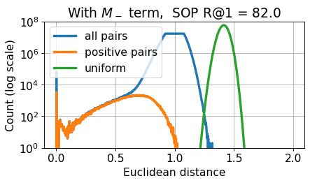
We defer the proof to Appendix B. This Proposition shows that is a valid ranking objective, similar to AP surrogates, multi-similarity, and triplet losses. Note that Proposition 4.1 does not hold for , since continues to provide gradients up to fixed margins, regardless of whether the correct ranking is satisfied. Figure 3 (left) shows that is approximately a linearly scaled version of 1-mAP over the course of training. Figure 3 (right) suggests that the value of converges when optimized using gradient descent. The Appendix contains more empirical evidence that the value of converges (Fig. 9 and 15 ). Figure 4 justifies the choice of heuristic gradient in Eq. 1. In this simple 2-D example, the gradient is always positive and non-zero in the direction away from the minimum, until the minimum is reached.

4.2 Intuition
In the previous subsection, we proved that the minimum of corresponds to a correct ranking of samples within a batch. We also showed that the value of converges empirically. However, we still need some intuition as to why gradients from work better than simple pair-wise contrastive loss functions. This discussion will naturally lead to the semantic consistency intuition promised at the beginning of the paper. Let us start by asking: what is the value of optimizing the intersection of neighborhood sets in the manner of Eq. 3? We offer a straight-forward intuition: Maximizing the intersection between the neighborhood sets of two samples is equivalent to pushing one sample towards the context of the other sample and vice versa; minimizing the intersection is equivalent to pulling apart the contexts of the two samples. We show this intuition by analyzing the gradient.
For simplicity, consider , such that the normalization factors in Eq. 3 are constant: and . For the remainder of the section we drop the subscript from for readability. Further consider a negative pair of samples and (), where is wrongly ranked w.r.t. (i.e. ). For the sake of developing intuition, let us further assume that all entries of are correct except index ; also, . Under these assumptions, and . This allows us to focus on interpreting Eq. 3. Under these assumptions, Eq. 3 simplifies to (see algebra in Appendix A):
| (8) |
and are positive constants, assuming that . denotes the inner product between the -th and -th rows of the indicator matrix. This inner product is clearly positive. must be a non-zero positive number under our assumptions. The gradient w.r.t. must be non-zero positive because . We are now ready for the backward pass. For simplicity of notation, denotes the gradient of the loss w.r.t. . The gradient w.r.t. the distance matrix can be split into two parts and , added together by chain rule.
| (9) |
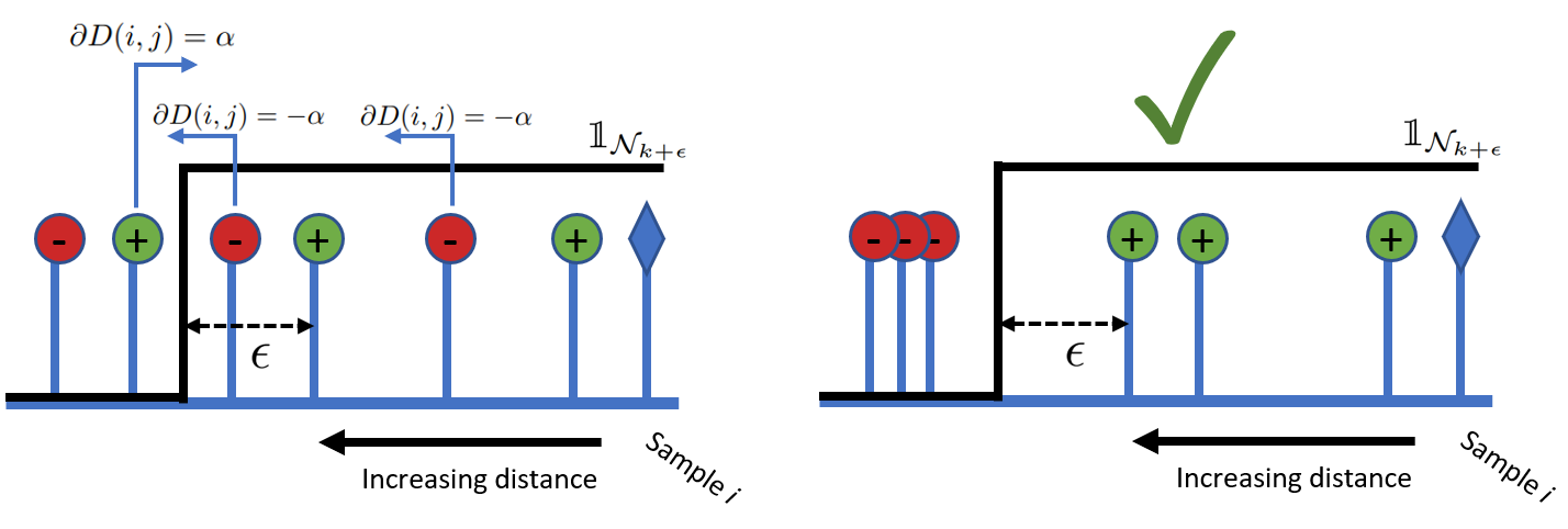
Note that the factors in Eq. 9 come from going backward through . The negative sign accounts for optimizing distance instead of similarity. Intuitively, the two components of the gradient perform different functions. The gradient in Eq. 9 enforces correct ranking. The gradient in Eq. 9 pulls away from the context of and away from the context of . More clearly, when and otherwise, for all samples in the batch. In words, we increase the distance between and all samples in the neighborhood of . See Figure 5 for an illustration.

4.3 Semantic Consistency
The previous subsection showed that the gradients of the contextual loss optimize distances between neighbors of samples, not just pairwise distances. This is important because the neighborhood of a sample contains semantically similar images, regardless of whether they have the same label or not. Indeed, optimizing contextual similarity may result in pulling apart samples with the same label, and to a lesser extent pushing together samples with different labels. For example, in Figure 5, sample is pulled both from sample , which has a different label, and from the two neighbors of sample , which have the same labels as sample .
This behavior is novel to the contextual loss. All of our baselines which take the cosine similarity matrix as input satisfy the condition that when and when . Note that this discussion is limited to pairwise ranking losses; classification methods cannot be analyzed in this way. We analyze the effect of these “wrong” gradients in Table 1 by adding a custom auto-grad function between the distance matrix and the contextual loss. This function truncates the gradient of the distance matrix according to the label matrix:
| (10) |
Clearly, clamping the distance gradients according to Eq. 10 raises the R@1 on training data at the expense of a lower test R@1. This raises the question: why does discarding seemingly wrong gradients lower the R@1 accuracy by 6%? We hypothesize that implicitly regularizes the embedding space against the label and image noise illustrated in Fig. 1. The contextual loss considers relationships between groups of samples, which intuitively should be more robust to random label variations than solely relying on pairwise relationships. In other words, sample pairs with gradients that violate the true labels are pairs where the is inconsistent with semantic information; these labels likely do not generalize to test data. We justify this hypothesis in the next section by testing the robustness and generalizability of our approach.
| CUB | with gradient correction | |
|---|---|---|
| Train R@1 | 87.0 | 92.9 |
| Test R@1 | 71.4 | 65.4 |

4.4 Robustness and Generalizability Experiments
The previous subsection proposed that optimizing contextual similarity with leads to an embedding space with higher test R@1 accuracy because contextual similarity is more robust to label noise and more generalizable to test data. We verify this claim with three sets of experiments on the CUB benchmark in Figure 6.
Label Noise We experiment with assigning random labels to 5, 10, and 20 % of randomly selected training samples.
Image Noise We scraped around 1,800 generic bird images from Bing using search terms such as “bird” and “flying bird”. We manually filtered the images such that each image contains at least one bird. We then replace a percentage of randomly selected CUB training samples with random images from our Bing dataset. This experiment simulates a typical web-scraped dataset, where images are often only lightly proofread by a human. In most modern image datasets, a small portion of labels are either wrong or do not accurately reflect the content of the image. We experiment with 5, 10, and 20 % image noise.
Limited Training Data According to traditional machine learning wisdom, small datasets are easier to overfit. We demonstrate that our method achieves reasonable results even when some training data is withheld. CUB-200 is already the smallest standard benchmark, with 5,994 training samples belonging to 100 classes. We experiment with using only the first 50, 60, 70, 80, and 90 classes for training.
The results from these three sets of experiments are presented in Fig. 6. Our method clearly outperforms other pairwise ranking losses. We tune learning rates individually for each method. We use batch size 256 and . We use by itself instead of the entire loss to study the contextual loss without additional regularization.
| CUB | Cars | |||||||||
| Method | R@1 | R@2 | R@4 | R@8 | mAP | R@1 | R@2 | R@4 | R@8 | mAP |
| DRML (Zheng et al. 2021) | 68.7 | 78.6 | 86.3 | 91.6 | - | 86.9 | 92.1 | 95.2 | 97.4 | - |
| DIML (Zhao et al. 2021) | 68.2 | - | - | - | - | 87.0 | - | - | - | - |
| DiVA (Milbich et al. 2020) | 69.2 | 79.3 | - | - | - | 87.6 | 92.9 | - | - | - |
| Proxy Anchor (Kim et al. 2020) | 69.7 | 80.0 | 87.0 | 92.4 | - | 87.7 | 92.9 | 95.8 | 97.9 | - |
| MS (Wang et al. 2019) | 67.8 | 77.8 | 85.6 | - | - | 87.8 | 92.7 | 95.3 | - | - |
| IBC (Seidenschwarz et al. 2021) | 70.3 | 80.3 | 87.6 | - | - | 88.1 | 93.3 | 96.2 | - | - |
| S2SD (Roth et al. 2020) | 70.1 | 79.7 | - | - | - | 89.5 | 93.9 | - | - | - |
| Proxy NCA + Metrix | 70.4 | 80.6 | 88.7 | - | - | 88.5 | 93.4 | 96.5 | - | - |
| PA + Metrix | 71.0 | 81.8 | 88.2 | - | - | 89.1 | 93.6 | 96.7 | - | - |
| MS + Metrix (Venkataramanan et al. 2021) | 71.4 | 80.6 | 86.8 | - | - | 89.6 | 94.2 | 96.0 | - | - |
| HIST (Lim et al. 2022) | 71.4 | 81.1 | 88.1 | - | - | 89.6 | 93.9 | 96.4 | - | - |
| MHGL (Ebrahimpour et al. 2022) | 70.6 | 80.9 | 88.0 | 92.3 | - | 90.1 | 94.2 | 96.4 | 98.1 | - |
| MS (Wang et al. 2019) | 65.9 | 76.6 | 84.9 | 90.8 | 36.1 | 82.1 | 88.6 | 92.9 | 95.7 | 35.7 |
| Contrastive (Hadsell et al. 2006) | 65.9 | 76.6 | 84.8 | 90.8 | 35.3 | 82.4 | 88.7 | 92.8 | 95.6 | 35.3 |
| Roadmap (Ramzi et al. 2021) | 66.0 | 76.8 | 85.3 | 91.1 | 36.0 | 83.5 | 89.8 | 93.7 | 96.3 | 37.3 |
| Triplet (Weinberger et al. 2005) | 64.8 | 75.9 | 84.5 | 90.6 | 33.8 | 88.1 | 93.1 | 96.0 | 97.7 | 41.8 |
| MS + miner (Wang et al. 2019) | 68.0 | 78.4 | 86.2 | 91.7 | 36.4 | 90.5 | 94.7 | 97.0 | 98.4 | 42.7 |
| Proxy Anchor (Kim et al. 2020) | 69.1 | 79.5 | 87.0 | 92.2 | 37.4 | 89.0 | 93.5 | 96.2 | 97.9 | 38.8 |
| Proxy NCA (Teh et al. 2020) | 66.3 | 77.1 | 85.5 | 91.5 | 35.1 | 88.2 | 93.2 | 96.1 | 97.9 | 38.2 |
| Contextual (Ours) | 71.9 | 81.5 | 88.5 | 93.1 | 40.2 | 91.1 | 95.0 | 97.1 | 98.4 | 43.3 |
| PA + AVSL (Zhang et al. 2022) | 71.9 | 81.7 | 88.1 | 93.2 | - | 91.5 | 95.0 | 97.0 | 98.4 | - |
| Contextual (Ours) | 72.7 | 82.2 | 88.8 | 93.4 | 40.5 | 91.8 | 95.4 | 97.4 | 98.6 | 43.3 |
| Method | R@1 | R@10 | R@100 | R@1000 |
|---|---|---|---|---|
| DRML | 79.9 | 90.7 | 96.1 | - |
| DIML | 79.3 | - | - | - |
| DiVA | 79.6 | 91.2 | - | - |
| Proxy Anchor | 79.1 | 90.8 | 96.2 | - |
| MS | 76.9 | 89.8 | 95.9 | - |
| IBC | 81.4 | 91.3 | 95.9 | - |
| S2SD | 80.0 | 91.4 | - | - |
| Proxy NCA + Metrix | 81.3 | 92.7 | 97.1 | - |
| PA + Metrix | 81.3 | 91.7 | 96.9 | - |
| MS + Metrix | 81.0 | 92.0 | 97.2 | - |
| HIST | 81.4 | 92.0 | 96.7 | - |
| MHGL | 81.7 | 92.0 | 96.6 | - |
| MS | 79.9 | 90.4 | 95.8 | 98.6 |
| Contrastive | 80.9 | 90.9 | 95.6 | 98.3 |
| Roadmap | 81.9 | 92.0 | 96.3 | 98.7 |
| Triplet | 81.9 | 92.5 | 96.8 | 98.9 |
| MS + miner | 82.2 | 92.5 | 96.7 | 98.8 |
| Proxy Anchor | 79.7 | 91.1 | 96.2 | 98.7 |
| Proxy NCA | 78.8 | 90.7 | 96.3 | 98.8 |
| Contextual (Ours) | 82.6 | 92.5 | 96.7 | 98.8 |
| PA + AVSL | 79.6 | 91.4 | 96.4 | - |
| Contextual (Ours) | 83.2 | 92.9 | 96.8 | 98.8 |

5 Experiments
Datasets We experiment on two small-scale and two large-scale datasets: Caltech-UCSD Birds (CUB-200) (Wah et al. 2011), Stanford Cars-196 (Krause et al. 2013), Stanford Online Products (SOP) (Oh Song et al. 2016), and mini-iNaturalist-2021 (Van Horn et al. 2018). CUB-200 and Cars-196 are smaller fine-grain classification datasets with 200 and 196 unique labels, respectively. SOP is a large-scale dataset with 120,053 product images from 22,634 classes. mini-iNaturalist-2021 is a subset of the iNaturalist-2021 species classification competition dataset, with 50 images from each of 10,000 species. iNaturalist results are deferred to Appendix G Table 4.
Baselines We compare against a diverse set of baselines in Tables 2 and 3. Some baselines (such as DRML, Metrix, S2SD, HIST, MHGL, and AVSL) use complicated tricks to achieve published results. We simply copy the results for these baselines from their original paper. We then choose a representative set of baselines which only modify the loss function, and reproduce their results under identical experimental conditions (indicated by in the tables). We first compare against contrastive and triplet losses, which are the accepted standard in the field. Multi-similarity (MS) is a popular pairwise ranking loss. From classification methods, we compare against proxy anchor and proxy NCA. From AP maximization methods, we compare against Fast-AP, Smooth-AP, and Roadmap (Fast-AP and Smooth-AP comparisons are deferred to Appendix G Table 4). The benchmark results for many of the above-mentioned loss functions are under-represented in the literature. For fair comparison, we tune learning rates separately for each loss function. We use default values for any other hyperparameters.
Hyperparameters and Setup On our method, we tune and separately for each dataset. We use fixed values for remaining hyperparameters: , , , , , . The results in the main paper all use 224224 image resolution. Some recent studies use 256256 image resolution; comparisons in this setting are included in Appendix G Table 4. We use Adam with a decaying learning-rate schedule. We report results on the model with the best test R@1 metric, as is standard in the literature. We tune learning rates separately for each method and dataset combination. We use a batch size of 256 for iNaturalist, 128 for SOP and CUB, and 64 for Cars; the larger batch size is necessary to achieve reasonable performance on iNaturalist, while the smaller batch size appears to reduce overfitting on Cars. We use a 4 per class balanced sampler. For SOP and iNaturalist, we use hierarchical sampling (Cakir et al. 2019), following prior work. We use an embedding size of 512 for most comparisons; we only use an embedding size of 1536 for comparison with AVSL. We use ResNet-50 with a linear embedding layer. For CUB and Cars, we add an additional linear projector layer, which is discarded at the end of training. We use GeM pooling (Radenović et al. 2018), a widely used generalization of max and mean pooling. We always freeze batch-norm. We emphasize that the setup described above is used for all baseline results marked by . Additionally, we add the linear projector and/or similarity regularization with only when it improves the baseline, for fair comparison.
Performance Metrics We report Recall @ for select . R@ is the percentage of test samples where at least one of the closest neighbors have the same label. We also report mAP, a standard ranking metric defined in Appendix I.3. We report the average of 6 trials on CUB and Cars, and 2 trials on SOP. We omit standard deviations for readability.
Discussion Our R@1 results are better than the best baseline across all datasets and embedding sizes. We achieve R@1 gains of 0.5%, 0.6 %, and 0.4 % on CUB, Cars, and SOP resp. for the 512 embedding size. We achieve gains of 0.8%, 0.3%, and 3.6% on these datasets for the 1536 embedding size. These results are an average of 6 trials with different random seeds on CUB and Cars, and 2 trials on SOP. Additionally, we achieve R@1 gains of 0.8%, 0.6%, 0.2%, and 0.3% over the best baseline on CUB, Cars, SOP, and iNaturalist, resp. averaged over 3 trials, under slightly different experimental settings using 256256 image resolution (see Table 4 in the appendix).
Ablation Figure 7 plots R@1 on CUB and Cars with different values of and . This figure shows that the best R@1 performance is always achieved by a combination of contextual and contrastive losses. The optimal value of is usually between 0.8 and 0.9. The similarity regularizer is only needed to achieve state-of-the-art on some datasets. This property is reasonable for a regularizer, and it is more important to observe that the similarity regularizer improves the results of many diverse metric learning losses (see Table 6 Appendix I.1).
6 Conclusion
In this work, we proposed a novel contextual loss based on contextual similarity optimization. Our contextual loss improves the R@1 performance significantly over the current state-of-the-art across four benchmarks, when regularized by the contrastive loss and a novel similarity regularizer. We established that our loss function reduces overfitting by regularizing the embedding space for semantic consistency among neighbors. We justified this interpretation both analytically by inspecting the gradient, and empirically by showing that our loss function is more robust to label noise. We carefully supported each component of our loss function through extensive experiments across two different experimental settings, accompanied by exhaustive ablation studies.
Ethics Statement
We note that metric learning can be applied to controversial problems such as person re-identification and face re-identification. Our work is mainly foundational, so does not contribute directly to these applications. We also limit our experimentation to the image retrieval aspect of metric learning.
Reproducibility Statement
Instructions on how to run the code is provided in a README file. We include details on hardware requirements in Appendix H.1. Code is released here: https://github.com/Chris210634/metric-learning-using-contextual-similarity
Acknowledgments
DISTRIBUTION STATEMENT A. Approved for public release. Distribution is unlimited. This material is based upon work supported by the Under Secretary of Defense for Research and Engineering under Air Force Contract No. FA8702-15-D-0001. Any opinions, findings, conclusions or recommendations expressed in this material are those of the author(s) and do not necessarily reflect the views of the Under Secretary of Defense for Research and Engineering.
References
- Arandjelović & Zisserman (2012) Arandjelović, R. and Zisserman, A. Three things everyone should know to improve object retrieval. In 2012 IEEE conference on computer vision and pattern recognition, pp. 2911–2918. IEEE, 2012.
- Brown et al. (2020) Brown, A., Xie, W., Kalogeiton, V., and Zisserman, A. Smooth-ap: Smoothing the path towards large-scale image retrieval. In European Conference on Computer Vision, pp. 677–694. Springer, 2020.
- Cakir et al. (2019) Cakir, F., He, K., Xia, X., Kulis, B., and Sclaroff, S. Deep metric learning to rank. In Proceedings of the IEEE/CVF conference on computer vision and pattern recognition, pp. 1861–1870, 2019.
- Cao et al. (2020) Cao, B., Araujo, A., and Sim, J. Unifying deep local and global features for image search. In European Conference on Computer Vision, pp. 726–743. Springer, 2020.
- Chang et al. (2021) Chang, D., Pang, K., Zheng, Y., Ma, Z., Song, Y.-Z., and Guo, J. Your” flamingo” is my” bird”: fine-grained, or not. In Proceedings of the IEEE/CVF Conference on Computer Vision and Pattern Recognition, pp. 11476–11485, 2021.
- Cho et al. (2014) Cho, K., Van Merriënboer, B., Bahdanau, D., and Bengio, Y. On the properties of neural machine translation: Encoder-decoder approaches. arXiv preprint arXiv:1409.1259, 2014.
- Chu et al. (2019) Chu, R., Sun, Y., Li, Y., Liu, Z., Zhang, C., and Wei, Y. Vehicle re-identification with viewpoint-aware metric learning. In Proceedings of the IEEE/CVF international conference on computer vision, pp. 8282–8291, 2019.
- Deng et al. (2019) Deng, J., Guo, J., Xue, N., and Zafeiriou, S. Arcface: Additive angular margin loss for deep face recognition. In Proceedings of the IEEE/CVF conference on computer vision and pattern recognition, pp. 4690–4699, 2019.
- Ebrahimpour et al. (2022) Ebrahimpour, M. K., Qian, G., and Beach, A. Multi-head deep metric learning using global and local representations. In Proceedings of the IEEE/CVF Winter Conference on Applications of Computer Vision, pp. 3031–3040, 2022.
- El-Nouby et al. (2021) El-Nouby, A., Neverova, N., Laptev, I., and Jégou, H. Training vision transformers for image retrieval. arXiv preprint arXiv:2102.05644, 2021.
- Ermolov et al. (2022) Ermolov, A., Mirvakhabova, L., Khrulkov, V., Sebe, N., and Oseledets, I. Hyperbolic vision transformers: Combining improvements in metric learning. In Proceedings of the IEEE/CVF Conference on Computer Vision and Pattern Recognition, pp. 7409–7419, 2022.
- Guillaumin et al. (2009) Guillaumin, M., Verbeek, J., and Schmid, C. Is that you? metric learning approaches for face identification. In 2009 IEEE 12th international conference on computer vision, pp. 498–505. IEEE, 2009.
- Hadsell et al. (2006) Hadsell, R., Chopra, S., and LeCun, Y. Dimensionality reduction by learning an invariant mapping. In 2006 IEEE Computer Society Conference on Computer Vision and Pattern Recognition (CVPR’06), volume 2, pp. 1735–1742. IEEE, 2006.
- Khrulkov et al. (2020) Khrulkov, V., Mirvakhabova, L., Ustinova, E., Oseledets, I., and Lempitsky, V. Hyperbolic image embeddings. In Proceedings of the IEEE/CVF Conference on Computer Vision and Pattern Recognition, pp. 6418–6428, 2020.
- Kim et al. (2020) Kim, S., Kim, D., Cho, M., and Kwak, S. Proxy anchor loss for deep metric learning. In Proceedings of the IEEE/CVF Conference on Computer Vision and Pattern Recognition, pp. 3238–3247, 2020.
- Kim et al. (2022) Kim, S., Kim, D., Cho, M., and Kwak, S. Self-taught metric learning without labels. In Proceedings of the IEEE/CVF Conference on Computer Vision and Pattern Recognition, pp. 7431–7441, 2022.
- Krause et al. (2013) Krause, J., Stark, M., Deng, J., and Fei-Fei, L. 3d object representations for fine-grained categorization. In Proceedings of the IEEE international conference on computer vision workshops, pp. 554–561, 2013.
- Lim et al. (2022) Lim, J., Yun, S., Park, S., and Choi, J. Y. Hypergraph-induced semantic tuplet loss for deep metric learning. In Proceedings of the IEEE/CVF Conference on Computer Vision and Pattern Recognition, pp. 212–222, 2022.
- Liu et al. (2016) Liu, Z., Luo, P., Qiu, S., Wang, X., and Tang, X. Deepfashion: Powering robust clothes recognition and retrieval with rich annotations. In Proceedings of the IEEE conference on computer vision and pattern recognition, pp. 1096–1104, 2016.
- McFee & Lanckriet (2010) McFee, B. and Lanckriet, G. R. Metric learning to rank. In ICML, 2010.
- Milbich et al. (2020) Milbich, T., Roth, K., Bharadhwaj, H., Sinha, S., Bengio, Y., Ommer, B., and Cohen, J. P. Diva: Diverse visual feature aggregation for deep metric learning. In European Conference on Computer Vision, pp. 590–607. Springer, 2020.
- Musgrave et al. (2020a) Musgrave, K., Belongie, S., and Lim, S.-N. A metric learning reality check. In European Conference on Computer Vision, pp. 681–699. Springer, 2020a.
- Musgrave et al. (2020b) Musgrave, K., Belongie, S., and Lim, S.-N. Pytorch metric learning, 2020b.
- Oh Song et al. (2016) Oh Song, H., Xiang, Y., Jegelka, S., and Savarese, S. Deep metric learning via lifted structured feature embedding. In Proceedings of the IEEE conference on computer vision and pattern recognition, pp. 4004–4012, 2016.
- Radenović et al. (2018) Radenović, F., Tolias, G., and Chum, O. Fine-tuning cnn image retrieval with no human annotation. IEEE transactions on pattern analysis and machine intelligence, 41(7):1655–1668, 2018.
- Ramzi et al. (2021) Ramzi, E., Thome, N., Rambour, C., Audebert, N., and Bitot, X. Robust and decomposable average precision for image retrieval. Advances in Neural Information Processing Systems, 34:23569–23581, 2021.
- Ramzi et al. (2022) Ramzi, E., Audebert, N., Thome, N., Rambour, C., and Bitot, X. Hierarchical average precision training for pertinent image retrieval. In Computer Vision–ECCV 2022: 17th European Conference, Tel Aviv, Israel, October 23–27, 2022, Proceedings, Part XIV, pp. 250–266. Springer, 2022.
- Ranjan et al. (2015) Ranjan, V., Rasiwasia, N., and Jawahar, C. Multi-label cross-modal retrieval. In Proceedings of the IEEE international conference on computer vision, pp. 4094–4102, 2015.
- Revaud et al. (2019) Revaud, J., Almazán, J., Rezende, R. S., and Souza, C. R. d. Learning with average precision: Training image retrieval with a listwise loss. In Proceedings of the IEEE/CVF International Conference on Computer Vision, pp. 5107–5116, 2019.
- Rolínek et al. (2020) Rolínek, M., Musil, V., Paulus, A., Vlastelica, M., Michaelis, C., and Martius, G. Optimizing rank-based metrics with blackbox differentiation. In Proceedings of the IEEE/CVF Conference on Computer Vision and Pattern Recognition, pp. 7620–7630, 2020.
- Roth et al. (2020) Roth, K., Milbich, T., Ommer, B., Cohen, J. P., and Ghassemi, M. S2sd: simultaneous similarity-based self-distillation for deep metric learning. arXiv preprint arXiv:2009.08348, 2020.
- Seidenschwarz et al. (2021) Seidenschwarz, J. D., Elezi, I., and Leal-Taixé, L. Learning intra-batch connections for deep metric learning. In International Conference on Machine Learning, pp. 9410–9421. PMLR, 2021.
- Sun et al. (2021) Sun, Y., Zhu, Y., Zhang, Y., Zheng, P., Qiu, X., Zhang, C., and Wei, Y. Dynamic metric learning: Towards a scalable metric space to accommodate multiple semantic scales. In Proceedings of the IEEE/CVF Conference on Computer Vision and Pattern Recognition, pp. 5393–5402, 2021.
- Teh et al. (2020) Teh, E. W., DeVries, T., and Taylor, G. W. Proxynca++: Revisiting and revitalizing proxy neighborhood component analysis. In European Conference on Computer Vision, pp. 448–464. Springer, 2020.
- Van Horn et al. (2018) Van Horn, G., Mac Aodha, O., Song, Y., Cui, Y., Sun, C., Shepard, A., Adam, H., Perona, P., and Belongie, S. The inaturalist species classification and detection dataset. In Proceedings of the IEEE conference on computer vision and pattern recognition, pp. 8769–8778, 2018.
- Venkataramanan et al. (2021) Venkataramanan, S., Psomas, B., Kijak, E., Amsaleg, L., Karantzalos, K., and Avrithis, Y. It takes two to tango: Mixup for deep metric learning. arXiv preprint arXiv:2106.04990, 2021.
- Wah et al. (2011) Wah, C., Branson, S., Welinder, P., Perona, P., and Belongie, S. The caltech-ucsd birds-200-2011 dataset. 2011.
- Wang et al. (2019) Wang, X., Han, X., Huang, W., Dong, D., and Scott, M. R. Multi-similarity loss with general pair weighting for deep metric learning. In Proceedings of the IEEE/CVF Conference on Computer Vision and Pattern Recognition, pp. 5022–5030, 2019.
- Weinberger et al. (2005) Weinberger, K. Q., Blitzer, J., and Saul, L. Distance metric learning for large margin nearest neighbor classification. Advances in neural information processing systems, 18, 2005.
- Weyand et al. (2020) Weyand, T., Araujo, A., Cao, B., and Sim, J. Google landmarks dataset v2-a large-scale benchmark for instance-level recognition and retrieval. In Proceedings of the IEEE/CVF conference on computer vision and pattern recognition, pp. 2575–2584, 2020.
- Wu et al. (2017) Wu, C.-Y., Manmatha, R., Smola, A. J., and Krahenbuhl, P. Sampling matters in deep embedding learning. In Proceedings of the IEEE international conference on computer vision, pp. 2840–2848, 2017.
- Yan et al. (2021) Yan, J., Luo, L., Deng, C., and Huang, H. Unsupervised hyperbolic metric learning. In Proceedings of the IEEE/CVF Conference on Computer Vision and Pattern Recognition, pp. 12465–12474, 2021.
- Yan et al. (2023) Yan, J., Luo, L., Deng, C., and Huang, H. Adaptive hierarchical similarity metric learning with noisy labels. IEEE Transactions on Image Processing, 32:1245–1256, 2023.
- Ye et al. (2021) Ye, M., Shen, J., Lin, G., Xiang, T., Shao, L., and Hoi, S. C. Deep learning for person re-identification: A survey and outlook. IEEE transactions on pattern analysis and machine intelligence, 44(6):2872–2893, 2021.
- Zhai & Wu (2018) Zhai, A. and Wu, H.-Y. Classification is a strong baseline for deep metric learning. arXiv preprint arXiv:1811.12649, 2018.
- Zhang et al. (2022) Zhang, B., Zheng, W., Zhou, J., and Lu, J. Attributable visual similarity learning. In Proceedings of the IEEE/CVF Conference on Computer Vision and Pattern Recognition, pp. 7532–7541, 2022.
- Zhao et al. (2021) Zhao, W., Rao, Y., Wang, Z., Lu, J., and Zhou, J. Towards interpretable deep metric learning with structural matching. In Proceedings of the IEEE/CVF International Conference on Computer Vision, pp. 9887–9896, 2021.
- Zheng et al. (2021) Zheng, W., Zhang, B., Lu, J., and Zhou, J. Deep relational metric learning. In Proceedings of the IEEE/CVF International Conference on Computer Vision, pp. 12065–12074, 2021.
- Zheng et al. (2022) Zheng, W., Huang, Y., Zhang, B., Zhou, J., and Lu, J. Dynamic metric learning with cross-level concept distillation. In Computer Vision–ECCV 2022: 17th European Conference, Tel Aviv, Israel, October 23–27, 2022, Proceedings, Part XXIV, pp. 197–213. Springer, 2022.
- Zhong et al. (2017) Zhong, Z., Zheng, L., Cao, D., and Li, S. Re-ranking person re-identification with k-reciprocal encoding. In Proceedings of the IEEE conference on computer vision and pattern recognition, pp. 1318–1327, 2017.
Appendix A Simplification of Step 2 in Main Paper Section 3
Under the assumption that , the formula for in terms of simplifies. We drop the subscript from for readability. When , there are exactly samples in the neighborhood set . Specifically, and . Eq. 3 becomes:
| (11) |
Under our assumptions, simplifies:
| (12) |
Note that , by definition. Eq. 11 becomes:
| (13) |
This can be written as Eq. 8 in the main paper, restated here:
| (14) |
Under the assumption that , and .
Appendix B Proof of Proposition 4.1
Forward direction If all samples are correctly ranked w.r.t. every other sample within the batch, show that .
Proof Recall that the Proposition assumes that there are exactly samples from each class in the batch. This means that the neighborhood set of every sample contains exactly the samples in the batch with the same label. In other words, . Further, if , then the inner product because the neighborhood sets of and are identical and there are exactly samples in this set.
When , . When , . Therefore, .
Following Eq. 4, it is also clear that when samples are correctly ranked. This is because, the neighborhood is a subset of the larger neighborhood. That is, if , then . Since , when , averaging the entries of over as indicated in Eq. 4 does not change . Therefore, . Finally, is symmetric, so . This proves that and by Eq. 5.
Backward direction If , show that all samples are correctly ranked w.r.t. every other samples within the batch.
Proof We prove this by contradiction. Suppose that and there exists a pair of samples , where is not correctly ranked w.r.t. . There are two possible cases: (1) but or (2) but . (1) is the case where and have the same label, but is not ranked as one of the top- neighbors of . (2) is the case where and have different labels, but is ranked as one of the top- neighbors of . Since we assume that there are exactly samples with the same label per batch, both (1) and (2) must be true. In particular, assume that (2) is true. Under Eq. 14, if , then because is multiplied by a non-zero positive number. Similarly, under Eq. 4, if , then because is multiplied by non-zero positive numbers and added to positive numbers. Since and , , which contradicts the assumption that and concludes the proof.

Appendix C Scalability
While the calculation of our loss function scales cubicly in time and space, GPU implementations of matrix multiplication are highly optimized. Consequently, our contextual loss remains practical even for batch sizes as high as 6400. See Figure 8. In comparison, AP surrogates such as Roadmap become impractical beyond batch sizes of about 2000. We used one A40 GPU for this experiment, so we were unable to plot points above 32 GB of GPU memory.

Appendix D Decomposability Gap
Ramzi et al. 2021 demonstrated mathematically the idea of a decomposability gap in their Roadmap paper. When optimizing a ranking metric such as AP, the average batch-wise AP is a loose upper bound of AP over the entire dataset. Given a reasonable embedding space (e.g. halfway through training), most randomly sampled batches are perfectly ranked, even if ranking over the entire dataset is far from optimal. Ramzi et al. 2021 call this difference between the batch-wise objective and the dataset-wise objective the “decomposability gap” and propose to use the standard contrastive loss to reduce this gap. The resulting optimization objective is a convex combination of the ranking loss and .
This decomposability gap could partially explain why we need to regularize with . Specifically, reaches a minimum of zero when all samples within a mini-batch are correctly ranked. At this point, the embedding no longer changes until an incorrectly-ranked mini-batch is sampled. This is problematic, because, without hard off-line sampling, the probability that a randomly sampled batch contains the “hard” triplet that is incorrectly ranked diminishes. This justifies the need for to complement our contextual loss. See Figure 9 for an empirical verification of the existence of a decomposability gap on the CUB dataset.
Appendix E Contextual Similarity Definition in Set Notation
In this section, we state the same contextual similarity definition as Section 3 in the main paper, but following the notation of Kim et al. 2022.
We compute the contextual similarity on a single batch, not the entire dataset. Two samples are contextually similar if they share the same neighbors, i.e. the intersection of their -neighbor sets is large. Following this intuition, we calculate , the preliminary contextual similarity between samples and :
| (15) |
| (16) |
We include in (so if , then includes two elements: and its closest neighbor). Then, we use query expansion and symmeterize to obtain the final contextual similarity. Query expansion (Arandjelović & Zisserman 2012) is a standard evaluation-time trick in metric learning. It boosts retrieval performance by retrieving neighbors of a sample’s neighbors. Analogously, we adjust the contextual similarity by averaging over the set of close reciprocal neighbors .
| (17) |
| (18) |
| (19) |
Note that and only depend on the cosine similarities between embeddings. We want to optimize the embeddings such that converges to . The value of is not arbitrary; it must be set to the number of samples per label in the mini-batch. For example, a standard metric learning setup is to randomly sample 32 labels and then sample 4 images per label. In this case, we set .
E.1 Differences with STML
This subsection enumerates in detail the technical differences between our definition of contextual similarity ( in Eq. 19) and the definition of contextual similarity in STML (Kim et al. 2022). Note that by necessity, we reference equations and notation in the STML paper.
- 1.
STML averages a non-linear function of the cosine similarity ( in their Eq. 5) with the contextual similarity ( in their Eq. 5) to arrive at an estimate of the ground-truth similarity. In their work, the resulting similarity is used to “teach” a student embedding network. In our work, the contextual similarity is optimized directly by the contextual loss , and the cosine similarity is directly optimized by the contrastive loss .
- 2.
We add a margin term to the neighborhood definition; STML uses . In our loss, the margin is necessary to encourage separation between embeddings with different labels.
- 3.
(Minor) We use the set of neighbors to calculate in our Eq. 16; STML uses the set of reciprocal neighbors to calculate in their Eq. 7.
- 4.
(Minor) We use the set of reciprocal neighbors for query expansion in our Eq. 18; STML uses the neighbors in their Eq. 8.
Additionally, our work contains the following technical innovations not found in (Kim et al. 2022):
- •
The implementation of contextual similarity in (Kim et al. 2022) involves indexing a matrix and setting those values to a constant. Consequently, the output depends on the input indirectly through an indexing operation. We re-implement the contextual similarity calculation in a way that only uses greater-than, logical-and, addition, and multiplication. A detailed explanation of this process is detailed in Appendix E.2 and E.3.
- •
We determine suitable differentiable substitutions for the logical-and and greater-than functions. logical-and could be replaced by simple averaging, multiplication, or . greater-than can be replaced by a sigmoid, a smooth upper-bound, or the constant-gradient heaviside. We ultimately chose to use multiplication and a constant-gradient heaviside. These two choices are intuitively motivated in Appendix E.2, Fig. 10, and experimentally justified in Table 5.
- •
E.2 Detailed Optimization Motivation
The definition in the previous sub-section clearly contains three discrete operations: (1) greater-than, (2) logical-and, and (3) intersection. For optimization, we will deal extensively with indicator matrices: we denote as the indicator matrix where for some set . We use to denote element-wise multiplication.
Greater-than This is used in Eq. 15 and 17 and is equivalent to the non-differentiable heaviside function . Our approach is to use the exact value of in the forward pass and a constant positive gradient in the backward pass. A constant positive gradient is reasonable since is a (non-strictly) increasing function.
| (20) |
In Section F.1 we show with a toy experiment that this approach is robust despite being somewhat heuristic. In contrast, is traditionally approximated by a sigmoid (e.g. for AP approximation and in Gated Recurrent Networks (Cho et al. 2014) ):
| (21) |
trades off the quality of the approximation with the domain where gradients are non-zero. As temperature decreases, approaches , but gradient vanishes everywhere except in a small region around the boundary. This behavior is not intuitive: it is undesirable to only have a large gradient at the boundary. Some prior work (e.g. ROADMAP) side-step this issue by using an upper-bound to the heaviside function (where the right side of the heaviside function increases linearly), which solves the gradient issue at the expense of grossly over-estimating the true objective. In our case, this is especially concerning since we will be multiplying together indicator functions. In Section G.1, we show that our approach in Eq. 20 achieves better empirical results than a sigmoid approximation.
Logical-and A logical-and is used explicitly in Eq. 18 and implicitly in Eq. 16 and 19. There are two differentiable substitutes for logical-and: and multiplication. Multiplication is smooth, but has no gradient at the origin. is logically consistent on the continuous domain [0,1], but the gradient is not continuous when inputs are equal. We found experimentally that multiplication is the best option, see row 5 of Table 5. A gradient of zero at the origin is desireable in the case of Eq. 18 and 19 (query expansion step). A work-around for the zero-gradient issue for Eq. 16 is presented in the next sub-section.
Intersection The number of elements in the intersection in Eq. 16 is calculated using matrix multiplication. A sample if . Using multiplication for the logical-and, the number of elements in the intersection can be expressed compactly as a function of the indicator matrices:
| (22) |
We are now ready to state the loss function by combining the definition of contextual similarity with the optimization method.
E.3 Loss in Matrix Notation
Our loss function straightforwardly combines the previous two sub-sections, with one exception for the intersection calculation in Eq. 16. Optimizing the intersection with tends to focus on pairs of neighboring samples because using multiplication for logical-and zeros out the gradient when both inputs are 0. This is problematic since the resulting embedding becomes clustered regardless of true similarity (see Figure 12). We mitigate this problem by optimizing the intersection of the complements in addition to optimizing the original intersection in Eq. 16. c denotes the complement of a set. Maximizing the size of the intersection between two sets is equivalent to maximizing the size of the intersection between their complements, and vice versa. This can be trivially proven under the assumptions that the universal set is constant and that the size of both sets is constant.

Let denote the matrix where is the squared Euclidean distance between the normalized features of sample and . . denotes stop gradient.
Step 1 (Neighborhood Optimization):
| (23) |
Step 2 (Optimizing Intersection of Neighborhoods):
| (24) |
Step 3 (Query Expansion):
| (25) |
| (26) |
| (27) |
Finally, we use the MSE loss to optimize against the true similarity labels :
| (28) |
is the key to our framework and works reasonably on its own. However, it has two vulnerabilities: (1) similar to learning to rank losses, can be small even if the distance between positive pairs is large, so long as there are no closer negative pairs (see Figure 10); (2) tends to converge to a solution where the average cosine similarity between all pairs is large, suggesting that only a small portion of the available embedding space is utilized. In response to problem (1), we add the standard contrastive loss ((Hadsell et al. 2006)), which explicitly optimizes the cosine similarity toward fixed margins and . In response to problem (2), we add a non-standard but straightforward similarity regularizer, which regularizes the average cosine similarity between all pairs toward a fixed value . Our final framework (Eq. 31) minimizes a weighted combination of the three losses.
| (29) |
| (30) |
| (31) |
Note that El-Nouby et al. 2021 propose a superficially similar similarity regularization scheme, which “maximizes the distance between every point and its nearest neighbor”. Our regularizes the average similarity between all pairs of samples. Nearest neighbor pairs are dominated by positive pairs, while all pairs are dominated by negative pairs. Therefore, our regularizer is fundamentally different from El-Nouby et al. 2021.
Appendix F Slightly Different Analysis
The contextual similarity loss function is highly non-trivial. In this section we demystify each of the three steps using a toy experiment and gradient analysis. This is a slightly different analysis than the one given in the main paper.
F.1 Step 1: Neighborhood optimization
Consider the following simplified version of :
| (32) |
This is a valid loss function that works reasonably on its own (see Figure 11). During each iteration, we sample a batch with exactly samples from each label. Intuitively, reaches a minimum of zero when includes only and the other samples with the same label, i.e. all samples are correctly ranked. Using the gradient of defined in Eq. 20, we see that negative samples which are in receive a gradient of magnitude pushing it away from , while positive samples which are not in receive a gradient of magnitude pushing it toward . See Figure 10.

F.2 Step 2: Optimizing Intersection of neighborhoods
While is a reasonable loss function already, row 1 of Table 5 shows that collapses without the contrastive loss (). We propose that this is because provides very sparse gradients: for most pairs. Consider the following more complicated loss:
| (33) |
is defined in Eq. 24. has two terms multiplied together element-wise. The term was already addressed in the previous sub-section, so we focus on the first term, which optimizes the intersection between neighborhood sets . We offer a straight-forward intuition: Maximizing the intersection between the neighborhood sets of two samples is equivalent to pushing one sample towards the context of the other sample and vice versa; minimizing the intersection is equivalent to pulling apart the contexts of the two samples. We show this intuition by analyzing the gradient.
For simplicity, consider , such that the normalization factors in Eq. 24 are equal to and , resp. Further consider a negative pair of samples and (), where is wrongly ranked w.r.t. (i.e. ). Following the loss function equations:
| (34) |
must be a non-zero positive number. Using the equation for , we see that the gradient w.r.t. must be positive because . We are now ready for the backward pass. For simplicity of notation, denotes the gradient of the loss w.r.t. .
| (35) |
Use the fact that and and vice versa:
| (36) |
| (37) |
Eq. 36 is the contribution to the gradient from optimizing , while Eq. 37 is the contribution to the gradient from optimizing . These can be added together:
| (38) |
Going backward through multiplies the gradient by (negative sign accounts for optimizing distance instead of similarity):
| (39) |
From the above equation, when and when , for all samples in the batch. In words, we increase the distance between and all samples in the neighborhood of , and we decrease the distance between and all points outside the neighborhood of . Recall that we assumed and to be a negative pair, so it makes sense to pull away from the context of in this fashion.
| CUB | Cars | |||||||
|---|---|---|---|---|---|---|---|---|
| Method | R@1 | R@2 | R@4 | R@8 | R@1 | R@2 | R@4 | R@8 |
| Contrastive | 68.5 0.3 | 78.3 0.1 | 86.0 0.2 | 91.3 0.1 | 85.4 0.2 | 91.1 0.3 | 94.6 0.3 | 96.8 0.1 |
| Triplet | 67.3 0.2 | 77.9 0.1 | 85.6 0.2 | 91.2 0.1 | 77.6 1.3 | 85.4 0.8 | 90.8 0.7 | 94.1 0.4 |
| NtXent | 65.7 0.4 | 76.3 0.2 | 84.3 0.4 | 90.0 0.4 | 79.0 0.6 | 86.0 0.3 | 91.0 0.2 | 94.4 0.3 |
| MS | 68.9 0.5 | 78.5 0.4 | 86.0 0.6 | 91.4 0.5 | 88.7 0.4 | 93.0 0.2 | 95.7 0.1 | 97.3 0.1 |
| N-Softmax | 61.3 | 73.9 | 83.5 | 90.0 | 84.2 | 90.4 | 94.4 | 96.9 |
| Proxy NCA ++ | 69.0 0.8 | 79.8 0.7 | 87.3 0.7 | 92.7 0.4 | 86.5 0.4 | 92.5 0.3 | 95.7 0.2 | 97.7 0.1 |
| Fast-AP | 63.3 0.1 | 73.7 0.4 | 82.2 0.3 | 88.5 0.2 | 74.7 0.4 | 82.5 0.7 | 88.0 0.6 | 92.2 0.2 |
| Smooth-AP | 66.5 0.9 | 76.6 0.5 | 84.8 0.6 | 90.8 0.4 | 81.1 0.2 | 87.8 0.4 | 92.2 0.3 | 95.1 0.3 |
| ROADMAP | 68.7 0.5 | 78.3 0.3 | 86.1 0.3 | 91.1 0.1 | 84.5 0.5 | 90.3 0.0 | 93.9 0.0 | 96.2 0.1 |
| Ours | 69.8 0.2 | 79.8 0.1 | 87.1 0.1 | 92.3 0.2 | 89.3 0.0 | 93.7 0.2 | 96.3 0.1 | 97.8 0.2 |
| SOP | mini-iNaturalist | ||||||
|---|---|---|---|---|---|---|---|
| Method | R@1 | R@10 | R@100 | R@1 | R@4 | R@16 | R@32 |
| Contrastive | 82.4 0.0 | 91.9 0.0 | 96.0 0.0 | 43.5 0.1 | 62.7 0.1 | 77.6 0.1 | 83.2 0.1 |
| Triplet | 82.0 0.0 | 92.5 0.1 | 96.7 0.0 | 35.4 0.1 | 56.5 0.1 | 74.7 0.1 | 81.7 0.1 |
| NtXent | 79.7 0.2 | 90.8 0.0 | 96.1 0.0 | 40.8 0.1 | 61.6 0.1 | 78.0 0.0 | 83.9 0.0 |
| MS | 81.4 0.0 | 91.4 0.0 | 96.1 0.1 | 44.9 0.1 | 63.9 0.1 | 78.4 0.1 | 83.9 0.1 |
| N-Softmax | 78.2 | 90.6 | 96.2 | – | – | – | – |
| Proxy NCA ++ | 80.7 0.5 | 92.0 0.3 | 96.7 0.1 | – | – | – | – |
| Fast-AP | 80.3 0.1 | 91.0 0.1 | 96.0 0.0 | 35.6 0.2 | 55.8 0.1 | 72.8 0.0 | 79.3 0.0 |
| Smooth-AP | 82.0 0.0 | 92.6 0.0 | 96.9 0.0 | 42.7 0.0 | 63.3 0.0 | 79.0 0.0 | 84.7 0.0 |
| ROADMAP | 83.1 0.1 | 92.6 0.0 | 96.6 0.0 | 45.9 0.1 | 65.8 0.0 | 80.4 0.1 | 85.7 0.0 |
| Ours | 83.3 0.0 | 92.9 0.1 | 96.7 0.0 | 46.2 0.0 | 65.8 0.1 | 80.2 0.1 | 85.4 0.1 |
F.3 Step 3: Query Expansion
Query expansion (QE) is an established trick for image retrieval (Arandjelović & Zisserman 2012). QE expands the neighborhood set by additionally retrieving the neighbors of very close neighbors. In the unsupervised setting, QE refers to averaging the contextual similarity scores for samples in the neighborhood (see Eq. 27); this leads to more robust pseudo-supervision. In our setting, we have two reasons for using QE (Eq. 25 26 and 27): (1) averaging with very close neighbors could have the same effect as label smoothing and (2) the neighborhood is optimized by Eq. 26 and 27. Empirically, QE is necessary to achieve the optimal performance of our framework, since achieves higher R@1 than in Table 5.
Appendix G 256 256 Resolution Experiments
We include 256 256 image resolution results in this section. This setup is slightly different from the main paper. These results are comparable to the results reported in the ROADMAP paper.
Hyperparameters and Setup on 256 256 Experiments We use hyperparameter values that are approximately optimal across all datasets. , , , , , , , . We follow the same training procedure as ROADMAP, but with a slightly faster learning-rate schedule for time efficiency. We use Adam with a learning-rate schedule that multiplies the learning rate by 0.3 at Epochs 15, 30, and 45. We train for 80 epochs. We report results on the model with the best test R@1 metric, as is standard in the literature. We use an initial learning rate of on CUB, on Cars, on SOP, and on iNaturalist. We use a batch size of 256 for iNaturalist and 128 for other datasets; the larger batch size is necessary to achieve reasonable performance on iNaturalist. We use a 4 per class sampler. For CUB and Cars, we use random sampling (sample 32 classes at random, then sample 4 images per class). For SOP and iNaturalist, we use hierarchical sampling (Cakir et al. 2019), following prior work. We use an embedding size of 512 and ResNet-50 with a linear embedding layer. Following prior work, we use layer-norm and max-pooling on the smaller CUB and Cars datasets. We always freeze batch-norm.
Discussion for 256 256 Experiments Our R@1 results are at least two standard deviations better than the best baseline across all datasets. Our results are especially good on CUB and Cars, where we achieve R@1 gains of 0.8% and 0.6 %, resp. We achieve more modest R@1 gains of 0.2% and 0.3% on SOP and iNaturalist, resp. We note that these gains are significant because the standard deviation is relatively small. We also note that while Proxy NCA ++ and MS are the best baselines on CUB and Cars, ROADMAP is the best baseline on SOP and iNaturalist. Our method is the best across all datasets, suggesting that it is more versatile.
| SOP R@1 | ||||
|---|---|---|---|---|
| Ablation () | Explanation | |||
| 83.13 | 41.99 | Eq. 32 (step 1 only) | ||
| 79.20 | 75.61 | Eq. 32 but using in Eq. 21 | ||
| 82.39 | 81.05 | Eq. 33 (skip step 3) | ||
| (skip step 2) | 82.74 | 81.74 | ||
| 66.57 | – | Use instead of for logical-and | ||
| 82.39 | 77.84 | Use for all steps | ||
| 82.31 | 80.72 | Remove term from Eq. 24 | ||
| No stop gradient in Eq. 24 | 73.03 | – | ||
| 83.20 | 82.04 | Final results without | ||
G.1 Ablation Results
In Table 5, we evaluate the contribution of each step in the calculation of . These experiments focus on dissecting , so we set (no similarity regularizer) and or . Overall, all of the modifications tested in Table 5 decrease the performance of in terms of R@1. In particular: row 1 shows that including only step 1 leads to a collapsed representation when ; rows 3 and 4 show that steps 3 and 2 of the loss calculation are necessary; row 7 shows that the term in Eq. 24 is necessary; rows 2 and 6 show that our approach to optimizing in Eq. 20 is better than using a sigmoid.
Appendix H Minor Experimental Details
H.1 Code and Environment
We include code with our submission. We run experiments on 1 V100 GPU with 16 GB of memory. The CUB and Cars experiments take under one hour. The SOP and iNaturalist experiments take 4 hours and 6 hours, respectively. Some of our code is borrowed from ROADMAP. For faster experimentation, we use mixed precision floating point. Experiments take more than 12 hours on P100 GPUs, partially because mixed precision arithmetic does not appear to speed-up experiments as much on P100 GPUs compared to on V100 GPUs.
H.2 Augmentation (Specific to 256 256 Experiments)
On CUB, Cars and SOP, we use random resized crop with default parameters to crop the image to 256 256 pixels. We horizontally flip the image with 50% probability. For testing, we resize the image to 288 pixels, then center crop to 256 pixels. On iNaturalist, we random resize crop to 224 224 pixels, then flip horizontally with 50% probability. We use a smaller image size on iNaturalist so that the larger batch size can fit in the 16 GB of GPU memory. For testing, we resize the image to 256 pixels then center crop to 224 pixels.
H.3 Sampling (Specific to 256 256 Experiments)
We use a batch size of 128 on CUB, Cars and SOP. We use a batch size of 256 on iNaturalist. On all datasets, we train for 80 epochs. An epoch is defined as 15, 30, 655, and 576 batches for CUB, Cars, SOP, and iNaturalist respectively. On CUB and Cars, we use a random 4 per class sampler. On SOP and iNaturalist, we use a balanced hierarchical sampling strategy, since there are super-labels. In particular, half of each batch is randomly sampled from one super-label, and the other half is randomly sampled from another super-label. In order to sample in a balanced manner (to prevent over-emphasis of uncommon super-labels), we arrange all samples in the training dataset into half-batches with same super-labels at the beginning of each epoch. We then form batches by pairing up half-batches in a round-robin fashion.
H.4 Loss Plot
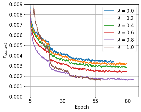
Figure 15 plots the contextual loss and test R@1 over the course of training on SOP, with varying . . These plots show that the loss decreases over the course of training; in general, a lower contextual loss corresponds to a higher test R@1. This result suggests that the contextual loss is a reasonable objective for image retrieval.
H.5 Note on Contrastive Loss
The contrastive loss has two margin parameters and . The optimal values for , the positive margin, is different depending on the value of (how much similarity regularization is used). For the “contrastive” results in row 1 of Table 4, we use and . For our results where , we set and . We find this tighter positive margin to be optimal under similarity regularization. However, we note that is likely to be too small when only the contrastive loss is used, since positive pairs are not encouraged to be more similar than a cosine similarity of 0.75.
H.6 Note on Stop Gradient
Note that we detach the normalization factors in Eq. 24. This is necessary because optimizing the size of the neighborhood is undesirable. On the contrary, we do not detach the normalization factor in Eq. 27. This is intentional even if somewhat un-intuitive. We show in Figure 17 that detaching in Eq. 27 increases R@1 on SOP when is high, but decreases R@1 in all other scenarios.
| Cars | |||||||||
|---|---|---|---|---|---|---|---|---|---|
| mAP | mAP@R | R@1 | |||||||
| Method | No | No | No | ||||||
| Contrastive | 38.2 | 40.6 +2.4 | 39.4 +1.2 | 28.8 | 31.2 +2.4 | 30.0 +1.2 | 85.4 | 88.0 +2.6 | 87.1 +1.7 |
| Triplet | 34.9 | 39.2 +4.3 | 38.5 +3.6 | 24.7 | 29.9 +5.2 | 29.2 +4.5 | 77.6 | 87.8 +10.2 | 86.7 +9.1 |
| NtXent | 36.2 | 37.0 +0.8 | 35.8 -0.4 | 26.3 | 27.0 +0.7 | 26.0 -0.3 | 79.0 | 79.9 +0.9 | 78.7 -0.3 |
| MS | 43.1 | 42.7 -0.4 | 43.6 +0.5 | 33.7 | 33.3 -0.4 | 34.1 +0.4 | 88.7 | 88.8 +0.1 | 89.3 +0.6 |
| Smooth-AP | 37.5 | 38.9 +1.4 | 38.1 +0.6 | 27.5 | 28.8 +1.3 | 28.2 +0.7 | 81.1 | 82.1 +1.0 | 82.4 +1.3 |
| ROADMAP | 38.3 | 39.2 +0.9 | 39.6 +1.3 | 28.7 | 29.6 +0.9 | 30.0 +1.3 | 84.5 | 85.7 +1.2 | 85.7 +1.2 |
| Ours | – | 42.4 | – | – | 33.0 | – | – | 89.3 | – |
| SOP | |||||||||
|---|---|---|---|---|---|---|---|---|---|
| mAP | mAP@R | R@1 | |||||||
| Method | No | No | No | ||||||
| Contrastive | 62.9 | 62.8 -0.1 | 62.7 -0.2 | 57.0 | 56.9 -0.1 | 56.8 -0.2 | 82.4 | 82.3 -0.1 | 82.3 -0.1 |
| Triplet | 63.1 | 64.4 +1.3 | 64.6 +1.5 | 56.4 | 57.8 +1.4 | 58.0 +1.6 | 82.0 | 83.1 +1.1 | 83.3 +1.3 |
| NtXent | 60.1 | 60.3 +0.2 | 60.0 -0.1 | 53.4 | 53.7 +0.3 | 53.4 +0.0 | 79.7 | 80.0 +0.3 | 79.7 +0.0 |
| MS | 62.5 | 62.4 -0.1 | 62.6 +0.1 | 56.2 | 56.1 -0.1 | 56.3 +0.1 | 81.4 | 81.4 +0.0 | 81.8 +0.4 |
| Smooth-AP | 63.1 | 63.2 +0.1 | 63.5 +0.4 | 56.4 | 56.5 +0.1 | 56.8 +0.4 | 82.0 | 82.1 +0.1 | 82.3 +0.3 |
| ROADMAP | 64.4 | 64.4 +0.0 | 64.4 +0.0 | 58.2 | 58.2 +0.0 | 58.2 +0.0 | 83.1 | 83.1 +0.0 | 83.1 +0.0 |
| Ours | – | 65.0 | – | – | 58.6 | – | – | 83.3 | – |
| iNaturalist | |||||||||
|---|---|---|---|---|---|---|---|---|---|
| mAP | mAP@R | R@1 | |||||||
| Method | No | No | No | ||||||
| Contrastive | 16.0 | 15.1 -0.9 | 15.5 -0.5 | 11.6 | 11.2 -0.4 | 11.5 -0.1 | 43.5 | 43.4 -0.1 | 43.7 +0.2 |
| Triplet | 12.1 | 13.3 +1.2 | 13.6 +1.5 | 7.9 | 9.8 +1.9 | 10.0 +2.1 | 35.4 | 41.4 +6.0 | 41.7 +6.3 |
| NtXent | 15.9 | 15.9 +0.0 | 15.9 +0.0 | 10.6 | 10.7 +0.1 | 10.6 +0.0 | 40.8 | 40.7 -0.1 | 40.7 -0.1 |
| MS | 16.6 | 16.6 +0.0 | 16.6 +0.0 | 11.9 | 11.9 +0.0 | 11.9 +0.0 | 44.9 | 44.9 +0.0 | 45.0 +0.1 |
| Smooth-AP | 16.5 | 16.6 +0.1 | 16.7 +0.2 | 11.3 | 11.4 +0.1 | 11.4 +0.1 | 42.7 | 43.1 +0.4 | 43.2 +0.5 |
| ROADMAP | 17.8 | 18.1 +0.3 | 18.0 +0.2 | 12.7 | 13.1 +0.4 | 13.0 +0.3 | 45.9 | 47.1 +1.2 | 46.8 +0.9 |
| Ours | – | 17.1 | – | – | 12.4 | – | – | 46.2 | – |
Appendix I Additional Experimental Results
I.1 Experimental Results on Similarity Regularizer
In the main paper, we presented the similarity regularizer as complementary to the contextual similarity loss . However, there is no theoretical reason for limiting the regularizer to our contextual similarity framework. We show in Table 6 that the similarity regularizer offers an improvement in retrieval performance when combined with some baselines. In particular, the regularizer consistently improves R@1 performance of Triplet, Multi-Similarity, Smooth-AP, and ROADMAP losses across Cars, SOP and iNaturalist benchmarks. This is a promising result.
I.2 In-Shop Results
We offer R@ results for standard values on the In-Shop dataset in Table 8. In-Shop ((Liu et al. 2016)) is a popular image retrieval benchmark. We use the standard train-test split: we use 25,882 images from 3,997 classes for training; for testing, we use a query set with 14,218 images and a gallery set (aka. reference set) with 12,612 images, both from 3,985 classes. We use the same augmentation and batch size as SOP. An epoch is defined as 600 batches.
I.3 Average Precision Results for Table 4
We offer Average Precision (AP) results in Table 7. We present results for two flavors of AP ((McFee & Lanckriet 2010)): mAP and mAP@R. mAP is the precision at , averaged across correctly retrieved samples, averaged across the query set. mAP@R ((Musgrave et al. 2020a)) only averages across retrievals up to the number of positive pairs in the gallery set. Hence, mAP@R is always smaller than mAP. The two versions of AP are equivalent bases for comparison. In the following equations, denotes the set of samples in the gallery set with the same label as query and denotes the set of samples in the gallery set with a different label than query . Prec@ denotes the precision at , which is the percentage of samples ranked less than or equal to with the same label as the query.




| CUB | Cars | SOP | mini-iNaturalist | |||||
|---|---|---|---|---|---|---|---|---|
| Method | mAP | mAP@R | mAP | mAP@R | mAP | mAP@R | mAP | mAP@R |
| Contrastive | 36.6 0.4 | 26.6 0.5 | 38.2 0.4 | 28.8 0.5 | 62.9 0.1 | 57.0 0.1 | 16.0 0.1 | 11.6 0.0 |
| Triplet | 36.9 0.4 | 26.5 0.2 | 34.9 0.8 | 24.7 0.7 | 63.1 0.0 | 56.4 0.0 | 12.1 0.0 | 7.9 0.0 |
| NtXent | 36.3 0.3 | 26.0 0.3 | 36.2 0.7 | 26.3 0.7 | 60.1 0.1 | 53.4 0.1 | 15.9 0.0 | 10.6 0.0 |
| MS | 38.0 0.1 | 27.7 0.1 | 43.1 0.3 | 33.7 0.3 | 62.5 0.0 | 56.2 0.1 | 16.6 0.0 | 11.9 0.0 |
| Fast-AP | 34.4 0.8 | 24.4 0.7 | 32.7 0.0 | 23.5 0.0 | 60.7 0.1 | 54.2 0.1 | 13.9 0.1 | 9.1 0.1 |
| Smooth-AP | 36.8 0.4 | 26.4 0.4 | 37.5 0.3 | 27.5 0.2 | 63.1 0.2 | 56.4 0.2 | 16.5 0.0 | 11.3 0.0 |
| ROADMAP | 37.7 0.1 | 27.5 0.2 | 38.3 0.4 | 28.7 0.4 | 64.4 0.1 | 58.2 0.1 | 17.8 0.0 | 12.7 0.0 |
| Ours | 38.3 0.2 | 28.0 0.2 | 42.4 0.4 | 33.0 0.3 | 65.0 0.1 | 58.6 0.1 | 17.1 0.0 | 12.4 0.0 |
| In-Shop | ||||||
|---|---|---|---|---|---|---|
| Method | R@1 | R@10 | R@20 | R@30 | R@40 | R@50 |
| Contrastive | 90.1 | 97.4 | 98.3 | 98.6 | 98.8 | 98.9 |
| Triplet | 90.2 | 98.0 | 98.7 | 99.0 | 99.2 | 99.3 |
| NtXent | 89.3 | 97.6 | 98.3 | 98.7 | 98.9 | 99.0 |
| MS | 86.9 | 96.1 | 97.3 | 97.9 | 98.1 | 98.3 |
| N-Softmax | 88.6 | 97.5 | 98.4 | 98.8 | – | – |
| Proxy NCA ++ | 90.4 | 98.1 | 98.8 | 99.0 | 99.2 | – |
| Fast-AP | 89.7 | 97.5 | 98.3 | 98.6 | 98.8 | 98.9 |
| Smooth-AP | 90.2 | 97.9 | 98.7 | 99.0 | 99.2 | 99.2 |
| ROADMAP | 90.4 | 97.6 | 98.3 | 98.6 | 98.8 | 99.0 |
| Ours | 90.7 | 97.8 | 98.5 | 98.9 | 99.1 | 99.2 |
I.4 Comparison on Hierarchical Retrieval Metrics
Over-reliance on binary supervision is a long-standing problem in metric learning which motivates our contextual loss. Another interesting line of work uses hierarchical labels during training to mitigate this over-reliance (Sun et al. 2021, Zheng et al. 2022, and Ramzi et al. 2022). These works fall under the umbrella of “dynamic metric learning” and “hierarchical metric learning”. One potential drawback of these works is their requirement for hierarchical labels, which may not always be available. Broadly speaking, hierarchical metric learning losses enforce a larger penalty on mistakes in discriminating between labels that are farther apart in the hierarchy during training. The resulting embedding space is more consistent in the sense that most retrieval mistakes are between labels close together in the hierarchy. For example, if the query is an image of a bird, any incorrectly retrieved images are likely to be birds from a closely related species, rather than images of other animals.
The contextual loss as presented in this paper does not use hierarchical labels, since our focus is advancing the state-of-the-art in fine-grained retrieval, irrespective of coarse-grained retrieval. Keeping this in mind, we offer results on hierarchical retrieval metrics in Table 9. From Table 9, we conclude that our contextual loss always achieves the highest fine-grained performance, but under-performs baselines at higher levels in the hierarchy. This trade-off in fine vs. coarse retrieval is consistent with results from HAPPIER (Ramzi et al. 2022). We hope that these results will be helpful for future work on adapting the contextual loss to the hierarchical retrieval setting.
| CUB | Cars | SOP | ||||||||
|---|---|---|---|---|---|---|---|---|---|---|
| Method | fine R@1 | fine AP | mid AP | coarse AP | fine R@1 | fine AP | coarse AP | fine R@1 | fine AP | coarse AP |
| Contrastive | 66.2 | 35.9 | 52.0 | 85.7 | 81.1 | 33.4 | 39.8 | 80.7 | 60.1 | 13.0 |
| Roadmap | 66.2 | 36.0 | 53.8 | 88.1 | 83.5 | 37.3 | 41.9 | 82.1 | 62.6 | 13.9 |
| Triplet | 65.0 | 34.5 | 53.8 | 89.8 | 89.3 | 43.3 | 42.7 | 81.8 | 62.5 | 15.0 |
| MS+miner | 69.4 | 37.4 | 53.5 | 88.5 | 90.7 | 42.7 | 39.4 | 82.1 | 63.2 | 13.5 |
| Proxy Anchor | 68.0 | 36.6 | 53.9 | 89.1 | 88.8 | 39.0 | 38.6 | 79.8 | 59.4 | 16.2 |
| Proxy NCA | 65.7 | 34.9 | 55.5 | 88.0 | 88.0 | 37.6 | 38.5 | 78.9 | 58.6 | 16.8 |
| Contextual (ours) | 72.7 | 40.3 | 54.3 | 86.4 | 91.0 | 43.4 | 39.1 | 82.7 | 63.7 | 13.5 |
I.5 Contextual Similarity Re-ranking at Test Time
Using contextual similarity for re-ranking at test time is a common trick used to improve recall accuracy. However, this is not a common evaluation setting, so we omitted it from the main paper. We offer R@1 results with contextual re-ranking in Table 10. The contextual re-ranking procedure is as follows. After training, we calculate the cosine similarity between all pairs of samples in the test set. Denote this as , for each pair of test samples and . We then calculate a simplified version of the contextual similarity between each pair of test samples and using Equations 15 and 16 in Appendix E. Note that while , so we need to rectify to occupy the same interval as . To this end, define . For retrieval, we use a weighted sum of the rectified cosine similarity and the contextual similarity: .
Table 10 shows that all methods benefit from contextual re-ranking, and our contextual loss remains the best method across the three benchmarks. Embeddings optimized by the contextual loss do not benefit more from contextual re-ranking than baselines (i.e. the relative increase in R@1 with contextual re-ranking is about the same across all methods). There is no theory to suggest that optimizing contextual similarity at train time results in better contextual similarity re-ranking at test time, and we make no claims regarding this.
| CUB | Cars | SOP | ||||||
|---|---|---|---|---|---|---|---|---|
| Method | no re-rank | no re-rank | no re-rank | |||||
| Contrastive | 66.2 | 66.6 | 66.8 | 81.1 | 81.2 | 80.8 | 80.7 | 81.0 |
| Roadmap | 66.2 | 67.4 | 66.9 | 83.5 | 83.5 | 83.3 | 82.1 | 82.3 |
| Triplet | 65.0 | 66.6 | 65.8 | 89.3 | 90.0 | 89.9 | 81.8 | 82.2 |
| MS+miner | 69.4 | 71.1 | 70.7 | 90.7 | 91.2 | 91.0 | 82.1 | 82.4 |
| Proxy Anchor | 68.0 | 69.1 | 69.0 | 88.8 | 89.3 | 89.1 | 79.8 | 80.1 |
| Proxy NCA | 65.7 | 67.2 | 66.9 | 88.0 | 88.5 | 88.5 | 78.9 | 79.1 |
| Contextual (ours) | 72.7 | 74.3 | 73.9 | 91.0 | 91.4 | 91.1 | 82.7 | 82.9 |
I.6 Additional Comparisons to AP Surrogates
Figures 18 through 29 present a comparison between our contextual loss function and various AP surrogates. The goal of these figures is to show that our contextual loss function is definitively better at ranking than AP surrogates. We optimize a convex combination of the ranking loss and standard contrastive loss. We present results for different choices of learning rates, (weight on ranking loss), and positive margin on the contrastive loss, since the optimal hyperparameters vary between methods. We include results for all three benchmarks. The AP surrogates included in this comparison are: Roadmap (Ramzi et al. 2021), Smooth-AP (Brown et al. 2020), Softbin-AP (Revaud et al. 2019), and Blackbox-AP (Rolínek et al. 2020).