Detectability of strongly lensed gravitational waves using model-independent image parameters
Abstract
Strong gravitational lensing of gravitational waves (GWs) occurs when the GWs from a compact binary system travel near a massive object. The mismatch between a lensed signal and unlensed templates determines whether lensing can be identified in a particular GW event. For axisymmetric lens models, the lensed signal is traditionally calculated in terms of model-dependent lens parameters such as the lens mass and source position . We propose that it is useful to parameterize this signal instead in terms of model-independent image parameters: the flux ratio and time delay between images. The functional dependence of the lensed signal on these image parameters is far simpler, facilitating data analysis for events with modest signal-to-noise ratios. In the geometrical-optics approximation, constraints on and can be inverted to constrain and for any lens model including the point mass (PM) and singular isothermal sphere (SIS) that we consider. We use our model-independent image parameters to determine the detectability of gravitational lensing in GW signals and find that for GW events with signal-to-noise ratios and total mass , lensing should in principle be identifiable for flux ratios and time delays .
I Introduction
The first direct detection of gravitational waves (GWs) from merging compact objects was reported by the LIGO and Virgo collaborations in 2016 Abbott et al. 2016. To date, Advanced LIGO Aasi et al. 2015 and Advanced Virgo Acernese et al. 2015 have reported about 90 events, most of which are mergers between stellar-mass black holes, during their first three observing runs Abbott et al. 2021a. Kamioka Gravitational Wave Detector (KAGRA) Somiya 2012; Aso et al. 2013; Akutsu et al. 2021 has joined the preexisting ground-based GW detectors to form the Advanced LIGO-Virgo-Kagra (LVK) network. The increased sensitivity of detectors such as LVK has allowed us to detect an increasing number of GW events and to perform various general relativistic and cosmological tests Abbott et al. 2021b; Collaboration et al. 2021. With the increasing sensitivity of the current ground-based detector network and future detectors such as the Cosmic Explorer (CE) Evans et al. 2021, the Einstein Telescope (ET) Maggiore et al. 2020, the Deci-Hertz Interferometer Gravitational Wave Observatory (DECIGO) Kawamura et al. 2021, and the Laser Interferometer Space Antenna (LISA) Barausse et al. 2020, the number of observed GW events will increase dramatically, as will the probability of observing new propagation effects such as gravitational lensing that have yet to be detected Abbott et al. 2021c.
When GWs travelling through the Universe encounter a massive object, such as a compact object, galaxy or galaxy cluster, that can act as a lens, deflection of these GWs, i.e. gravitational lensing, will occur Lawrence 1971; Ohanian 1974; Nakamura and Deguchi 1999; Nakamura 1998; Takahashi and Nakamura 2003; Oguri 2018a; Li et al. 2018. Strong lensing of GWs will arise when a lens is very close to the line of sight. This will result in the GWs splitting into different lensed images, each with its own magnification and phase Takahashi and Nakamura 2003; Ezquiaga et al. 2021. There will also be an associated time delay between the lensed images which could range from seconds to years depending on the mass of the lens and geometry of the lens system Schneider 1985; Schneider et al. 1992.
GW lensing, if detected, could facilitate several exciting scientific studies. It could be used to extract information about the existence of intermediate-mass (mass ranging from - ) Lai et al. 2018 or primordial black holes Diego 2020; Oguri and Takahashi 2020 and test general relativity Baker and Trodden 2017; Collett and Bacon 2017; Mukherjee et al. 2020, including through constraints from GW polarization content Goyal et al. 2021. In addition, if a lensed electromagnetic (EM) counterpart of the lensed GW event is observed, it could help to locate the host galaxy at sub-arcsecond precision Hannuksela et al. 2020. Combining the information from the two messengers, i.e. GW and EM lensing, could enable high-precision cosmography Sereno et al. 2011; Liao et al. 2017; Cao et al. 2019; Li et al. 2019; Yu et al. 2020; Wempe et al. 2022.
There are two major differences between the gravitational lensing of EM waves and GWs from the point of view of wave-optics effects. The first difference is in the applicability of the geometrical-optics approximation. In the case of EM waves, this approximation, typically valid when the wavelength of the waves is much smaller than the Schwarzchild radius of the lens, applies to the vast majority of observations. This is not always the case for GWs, since ground-based detectors such as the LVK network observe at frequencies — Hz, lower than even the lowest-frequency radio telescopes. These GWs have wavelengths longer than the Schwarzschild radii of lenses with masses , leading to non-negligible wave-optics effects. The second difference is that the GWs emitted by compact binaries, unlike most EM sources, are coherent, causing interference between lensed images when the signals overlap at the observer.
In this paper, we focus on strong gravitational lensing by stellar-mass objects and GW sources consistent with those seen by the LVK network. However, our treatment is also applicable to more massive lenses, and to sources such as supermassive binary black holes that will be detectable by LISA. In the frequency domain, the modulation of GWs due to gravitational lensing is characterized by a multiplicative factor known as the amplification factor. Typically, this factor is parameterized in terms of model-dependent lens parameters such as the source position and lens mass Nakamura and Deguchi 1999; Takahashi and Nakamura 2003. In the limit where the geometrical-optics approximation is valid, for a particular axisymmetric lens model, analytical equations relate these lens parameters to a set of model-independent image parameters, the flux ratio and time delay between the images. Motivated by current GW search pipelines which use unlensed GW templates, we explore the detectability of lensing signatures using a match-filtering analysis between lensed GW source and unlensed GW templates. For the axisymmetric lens models, we explore the mismatch between the lensed and unlensed GW waveforms in both the lens and image parameter spaces.
This paper is organized as follows. In Sec. II, we begin with a pedagogical outline of gravitational lensing of GWs, discussing the time delay and amplification factor due to the lens. We then present the prescription used to generate the GWs in the inspiral phase of binary compact objects using the post-Newtonian approximation following Cutler and Flanagan 1994. In Sec. III, we present a detailed analysis of the point mass (PM) and singular isothermal sphere (SIS) axisymmetric lens-mass profiles and introduce the model-independent image parameters. In Sec. IV, we perform a match-filtering analysis in which we calculate the mismatch between lensed and unlensed GWs. Appendices A and B investigate the mismatch between lensed GW source and unlensed templates. Throughout the paper, we assume .
II Basic formalism
In this section, we briefly review the basic theory of the gravitational lensing of GWs.
II.1 Gravitational lensing

In the strong gravitational-lensing regime, we observe multiple images (or a single very distorted image) of a distant background source due to the presence of an intervening massive astrophysical object known as a lens. Lensing occurs when the GWs from a compact binary system travel near a lens as shown for the general lensing geometry in Fig. 1 Schneider et al. 1992. The extents of the lens and the source are taken to be much less than the observer-lens and lens-source distances, in which case they can be localized to the lens and source planes. An optic axis connects the observer and the center of the lens. The lens and source planes are at angular-diameter distances and respectively. The angular-diameter distance between the lens and source planes is . A GW source is located on the source plane at displacement with respect to the optic axis. After being emitted by the source, the GWs travel to the lens plane, with an impact parameter , and are deflected through an angle by the gravitational potential of the lens. and are dimensionless vectors on the lens and source plane respectively, where is a model-dependent characteristic length scale on the lens plane called the Einstein radius. GWs that reach the observer satisfy the lens equation
| (1) |
where
| (2) |
is the scaled deflection angle at the observer. The lensing potential is given by the two-dimensional Poisson equation
| (3) |
where is the surface mass density of the lens and is the critical surface mass density. For the formation of multiple images, is a sufficient, but not necessary condition Subramanian and Cowling 1986.
Gravitational lensing causes a time delay between the lensed images at the observer. The arrival time has two components, one arising from the geometry of the path traveled, and the other due to the gravitational potential of the lens known as the Shapiro time delay. The time delay at the observer due to a lens at redshift is
| (4) |
where is chosen such that the minimum value of the time delay is 0.
The lensing amplification factor relates the lensed waveform to the unlensed waveform for GWs of frequency . It is given by Kirchhoff’s diffraction integral Schneider et al. 1992; Takahashi and Nakamura 2003
| (5) |
This integral over the lens plane accounts for all the trajectories in which the wave can propagate; it is unity in the absence of a lens.
II.1.1 Geometrical-optics approximation
In the geometrical-optics approximation, generally valid for GW frequencies and lens masses for which Takahashi 2004, discrete images form at the stationary points of the time-delay function at which . Only these points contribute to the lensing amplification factor
| (6) |
where is the magnification of the image and the Morse index has values of 0, 1/2, or 1 depending on whether is a minimum, saddle point, or maximum respectively of the time-delay surface, .
II.2 Gravitational waveform
We restrict our analysis to the inspiral phase of the GW evolution from binary black hole (BBH) mergers and use the post-Newtonian (PN) approximation to model our unlensed waveform Cutler and Flanagan 1994
| (7) |
where is the the luminosity distance to the source, is the GW phase, and the GW amplitude is a function of sky localization and source geometry of order unity as discussed in Apostolatos et al. 1994. For a BBH system with masses and , is the total mass, is the symmetric mass ratio, is the redshifted total mass, and is the redshifted chirp mass. The cutoff frequency is chosen to be twice the orbital frequency at the innermost stable circular orbit of a BH of mass .
To 1.5PN order Cutler and Flanagan 1994, the GW phase is
| (8) |
where and are the coalescence time and phase and is the PN expansion parameter.
III Axisymmetric lens models
In this section, we discuss two axisymmetric lens models, the singular isothermal sphere (SIS) and the point mass (PM), that produce at most two images in the geometrical-optics approximation. We introduce model-independent image parameters that describe the amplification factor in this approximation, and assess the validity of these new parameters as the geometrical-optics approximation breaks down at low frequencies.
III.1 Singular isothermal sphere (SIS)
The SIS density profile , where is the velocity dispersion, is the most simple profile that can effectively describe the flat rotation curves of galaxies Gavazzi et al. 2007. It leads to the lensing potential by Eq. (3) and the amplification factor Takahashi and Nakamura 2003; Matsunaga and Yamamoto 2006
| (9) |
by Eq. (5), where , , is the Bessel function of zeroth order, is the Einstein radius, and is the lens mass inside the Einstein radius.
III.2 Point mass (PM)
The PM is the simplest mass distribution for a gravitational lens. It leads to a lensing potential and amplification factor Peters 1974; Takahashi and Nakamura 2003
| (10) |
where , , , and is the confluent hypergeometric function. The Einstein radius for a PM of lens mass is .
III.3 Geometrical-optics approximation
In the limit where the geometrical-optics approximation is valid, a source at position creates a discrete number of images at positions which are stationary points of the time delay given by Eq. (4). For the SIS lens, only one image is formed if the source is outside the unit circle (), whereas two images are formed if the source is inside (). The amplification factor in the geometrical-optics approximation of Eq. (6) is given by Takahashi and Nakamura 2003
| (11) |
where
| (12a) | ||||
| (12b) | ||||
As a PM lens can deflect photons by an arbitrarily large angle for sufficiently small impact parameter, there are two images for all source positions . is given by Takahashi and Nakamura 2003
| (13) |
where
| (14a) | ||||
| (14b) | ||||
Both the SIS and PM lens models can be parameterized by two lens parameters, the source position and lens mass .
The amplification factor for the SIS is shown in Fig. 2. In the low-frequency limit, converges to unity because diffraction effects prevent long-wavelength GWs from being affected by the presence of a lens Bontz and Haugan 1981; Takahashi and Nakamura 2003. In the high-frequency limit, the geometrical-optics approximation is valid and oscillatory behavior is observed due to interference between the coherent lensed images. We assume that the time delay is much less than the observing time of the GW detector as is appropriate for the lens mass shown in Fig. 2.
Fig. 3 shows the unlensed waveform and lensed waveform as functions of frequency . The unlensed waveform given by Eq. (7) is parameterized by the GW amplitude , redshifted chirp mass , symmetric mass ratio , source luminosity distance , coalescence time , and coalescence phase ; we choose fiducial values of , , , , and Gpc for these source parameters. It is proportional to according to Eq. (7) and appears as a straight line in this log-log plot. The lensed waveform is calculated for a SIS with lens parameters and and displays oscillatory behavior due to interference between the two terms in Eq. (11).
III.4 Model-independent image parameters
When the amplification factor is given by Eq. (13), i.e. the source position is such that two images are formed and the geometrical-optics approximation is valid, we can express this factor directly in terms of the flux ratio and time delay between the images. These “image parameters” are model-independent in that they fully specify the amplification factor for any two-image lens model up to an overall normalization that is observationally degenerate with the GW amplitude . The relationship between these image parameters and lens parameters like the source position and lens mass is model dependent; these relations for the SIS and PM lens models are given by Eqs. (12) and (14) respectively.
In Fig. 4, we plot the flux ratio and time delay as parametric functions of the source position for our two axisymmetric lens models and two choices of the lens mass . The blue cross indicates specific, potentially observable values ( and s) of the model-independent image parameters. According to Eqs. (12) and (14), these values can be obtained in both the SIS and PM lens models, albeit with different lens parameters, and for the SIS lens and and for the PM lens. This analysis reveals that apart from any observational errors associated with measuring the image parameters and , there is a model dependence with which lens parameters like and can be reconstructed.
IV Matched-filtering analysis
In this section, we perform a matched-filtering analysis to quantify the difference between lensed and unlensed GWs. The mismatch between two waveforms and is defined as Cutler and Flanagan 1994
| (15) |
The noise-weighted inner product between the waveforms and is defined as
| (16) |
where is the noise power spectral density (PSD). We use the pycbc.filter package Nitz et al. 2022 to evaluate the mismatch between waveforms. The two waveforms and can be distinguished when their mismatch , where is the signal-to-noise ratio (SNR) of a waveform Finn 1992; Finn and Chernoff 1993; Cutler and Flanagan 1994.
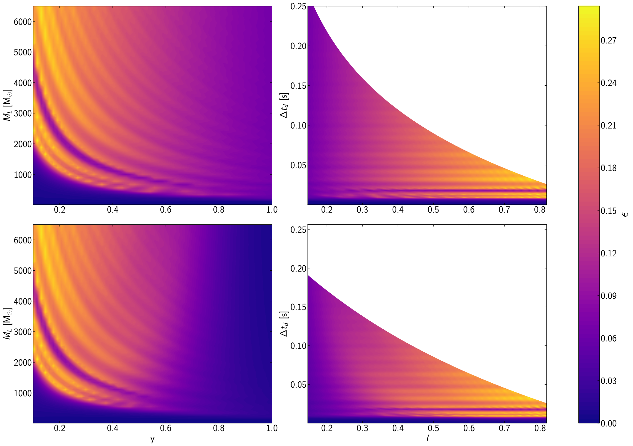
Fig. 5 shows contour plots of the mismatch between lensed GW source and unlensed templates as functions of the model-dependent lens parameters and (left panels) and the model-independent image parameters and (right panels) for PM lenses (top panels) and SIS lenses (bottom panels). We use the same source parameters for the lensed and unlensed templates and the noise PSD appropriate for a single two-armed detector with aLIGO design sensitivity. The mismatches as functions of the lens parameters are qualitatively similar for the PM (top left panel) and SIS (bottom left panel) models. For a vanishing lens mass (), diffraction causes the amplification factor to approach unity () and the mismatch to vanish () according to Eq. (15) for . The biggest difference between the two models occurs in the limit , where for the SIS model according to Eq. (12a) but for the PM model according to Eq. (14a). This accounts for the much smaller mismatches for the SIS model compared to the PM model in this limit.
The PM and SIS models become qualitatively indistinguishable when the mismatch is expressed as a function of the image parameters of and as shown in the right panels of Fig. 5. Although the top and bottom panels appear the same in the regions where they overlap, the PM model extends to larger values of the time delay than the SIS model at small flux ratios . This occurs because the mappings Eqs. (12) and (14) between the lens parameter space in the left panels and the image parameter space in the right panels are model-dependent.
The better agreement between the mismatches in the PM and SIS lens models when expressed as functions of the image parameters and can be seen even more clearly in Fig 6. This figure shows the difference between the mismatches for PM and SIS lens models shown in the top and bottom panels of Fig. 5. The left panel of Fig 6 shows large differences between the two lens models for source distances where the flux ratio vanishes in the SIS model but not the PM model. However, when the mismatch difference is expressed as a function of the image parameters in the right panel, the amplification factors and thus the mismatches only have significant differences for s where the geometrical-optics approximation breaks down.

The right panels of Fig. 5 also reveal that the crests and troughs of the oscillations in occur on lines of constant time delay . We examine these oscillations and the general dependence of the mismatch on our lens and image parameters for the SIS model in Fig. 7. The top left (right) panels of Fig. 7 show vertical (horizontal) slices of the bottom left panel of Fig. 5 along lines of constant (). The dependence of the mismatch on these lens parameters is non-monotonic and difficult to interpret, exhibiting oscillations of varying amplitude, frequency, and phase and a deep valley. The dependence of on the image parameters and shown in the bottom panels is far easier to interpret. The bottom left panel shows that in the diffraction limit , while in the opposite extreme geometrical-optics limit , as derived in Appendix A. The crests and troughs of the oscillations, as well as the deep valley at s are all aligned in this panel, reinforcing our contention that these oscillations are purely functions of the time delay . They are absent in the bottom right panel, where is held constant and the mismatch depends smoothly on the flux ratio in reasonable agreement with the extreme geometrical-optics limit .
We investigate the oscillations in the mismatch as a function of the time delay in Appendix B. These oscillations result from the number and location of the peaks of the amplification factor shown in Fig. 2 within the sensitivity band of the detector changing as varies. For our approximate waveform of Eq. (7), the sharpest feature in the detector response is a cutoff in the strain above a frequency . According to Eq. (24), this cutoff couples to the peaks of the amplification factor to create oscillations in the mismatch with frequency as a function of the time delay with frequency and amplitude proportional to . Numerical-relativity simulations reveal that true waveforms transition smoothly to a ringdown rather than experiencing such a sharp cutoff Mroue et al. 2013; Aasi et al. 2014; Boyle et al. 2019, but the merger should still imprint a feature leading to oscillations in the mismatch between a lensed GW source and unlensed templates. Our analysis suggests that these oscillations may be significant for large flux ratios (small source distances ), implying that serendipity between the lens parameters and source mass may facilitate the discovery of lensing in GW events.
V Discussion
In the geometrical-optics approximation, strong gravitational lensing produces multiple images. The lensing amplification factor can be expressed as a summation over these images, each with its own magnification , time delay , and Morse index as given by Eq. (6). In any given lens model, these “image parameters” can be calculated as functions of the “lens parameters” such as the source position and the lens mass . We propose that observational searches for strong lensing in GW events, as well as theoretical studies of their feasibility, should be conducted in terms of these model-independent image parameters rather than the model-dependent lens parameters. Separating detection and parameter estimation/model selection into distinct stages of GW data analysis should clarify the challenges of each stage as well as reduce their associated computational costs.
In this paper, we investigate this proposal by considering two well-known axisymmetric lens models: the singular isothermal sphere (SIS) and the point mass (PM). The SIS model has a density profile appropriate for a galaxy or stellar cluster, while the PM model could describe an individual star or compact object. In the geometrical-optics approximation, the SIS produces two images for source positions , while the PM always produces two images. For the case of two images, the amplification factor is given by Eq. (13) for both models, but the mappings between the image parameters (the flux ratio and the time delay ) and the lens parameters (the source distance and the lens mass ) are model dependent and given by Eqs. (12) and (14) respectively. This implies that uncertainty in the lens model will translate into uncertainty in the lens parameters, even if the image parameters could be measured with arbitrary precision. We illustrate this in Fig. 4, where the SIS and PM models can generate images with identical flux ratios and time delays despite have lens parameters that differ by . This represents a conservative estimate of the systematic error in the lens parameters associated with uncertainty in the lens model, as the PM model is more compact than any real galaxy or halo.
Lensed GW events with finite signal-to-noise ratios can be distinguished from unlensed templates if the minimum mismatch between the lensed signal and members of the template bank exceeds Finn 1992; Finn and Chernoff 1993; Cutler and Flanagan 1994. The oscillatory features induced in the waveform by lensing in the geometrical-optics limit depicted in Fig. 3 have little degeneracy with the source parameters specifying the unlensed waveform in Eqs. (7) and (II.2), so we approximate this minimum mismatch by that between lensed and unlensed waveforms with the same source parameters. In this approximation, the mismatch can be approximated by according to Eq. (21) and lensing should in principle be identifiable for flux ratios and time delays . We further showed in the right panel of Fig. 6 that the amplification factor of Eq. (13) is an excellent approximation to both the SIS and PM lens models in the geometrical-optics limit, suggesting that it should be suitable for model-independent searches for strong lensing in GW events.
Although gravitational lensing has not been detected in any of the GW events observed in the first three runs of the LVK detector network Abbott et al. 2021c, recent estimates Oguri 2018b suggest that strongly lensed GW events could be observed each year by future third-generation detectors like the proposed Cosmic Explorer (CE) Evans et al. 2021 and Einstein Telescope (ET) Maggiore et al. 2020. The detection of gravitational lensing in GW events would be of tremendous scientific interest because it could test general relativity Baker and Trodden 2017; Collett and Bacon 2017; Mukherjee et al. 2020, probe the distribution of dark matter Guo and Lu 2022; Cao et al. 2022, and improve the precision of cosmological constraints Goyal et al. 2021 We propose that GW templates based on model-independent image parameters will be a valuable tool in this effort. In upcoming studies, we will investigate how effectively these GW templates can be used to identify additional images created by non-axisymmetric lenses Ali et al. 2022 and distinguish the effects of lensing from those of spin precession Stoikos et al. 2022.
Acknowledgements
This work is supported by National Science Foundation Grant No. PHY-2011977. The authors thank Christina McNally for discussions. The authors acknowledge the Texas Advanced Computing Center (TACC) at The University of Texas at Austin for providing HPC resources that have contributed to the research results reported within this paper Stanzione et al. 2017. URL: http://www.tacc.utexas.edu
Appendix A Mismatch in the extreme geometrical-optics limit
We define the overlap between a lensed waveform and unlensed template as
| (17) |
For a lensed waveform with the amplification factor of Eq. (13) appropriate for a two-image lens in the geometrical-optics approximation and an unlensed waveform with the same source parameters, this overlap becomes
| (18) |
where
| (19a) | ||||
| (19b) | ||||
| (19c) | ||||
In the extreme geometrical-optics limit , the oscillatory terms do not contribute to the integrals implying , , and
| (20) |
where is the flux ratio between the two images. Although the match 1 - is normally calculated by maximizing the overlap over the coalescence time and phase as in Eq. (15), it is independent of these parameters in the limit . This implies that the mismatch takes the limiting value
| (21) |
Appendix B Investigating oscillations in the mismatch
In this Appendix, we examine the oscillations in the mismatch as a function of the time delay seen in the bottom left panel of Fig. 7. We reproduce the curve from this figure in Fig. 8 above. In the geometrical-optics approximation, lensing induces an oscillatory contribution to the GW phase that is poorly matched by a linear change to the GW phase resulting from a shift in the coalesence time and phase according to Eq. (II.2). As such, the mismatch is well approximated as , where the overlap is given by Eqs. (17) - (19). The crests and troughs of the oscillations in the mismatch as a function of the time delay will therefore occur where
| (22) |
vanishes. We show further that
| (23a) | ||||
| (23b) | ||||
| (23c) | ||||
where we have defined , approximated by a constant in angular brackets equal to its average value, and assumed as will be true for small redshifted source masses in the geometrical-optics limit. Inserting these into Eq. (22) and using the extreme geometrical-optics approximation described in Appendix A, we find
| (24) |
This result implies that the crests [troughs] in the mismatch will occur at time delays [] for which [], i.e.
| (25a) | ||||
| (25b) | ||||
| Crests | Troughs | |||
|---|---|---|---|---|
| Numerical [ms] | Predicted [ms] | Numerical [ms] | Predicted [ms] | |
| 1 | 11.51 | 10.47 | 15.91 | 15.71 |
| 2 | 21.31 | 20.94 | 26.12 | 26.18 |
| 3 | 32.52 | 31.41 | 36.72 | 36.65 |
| 4 | 42.13 | 41.88 | 47.33 | 47.12 |
| 5 | 53.53 | 52.36 | 57.13 | 57.59 |
| 6 | 63.54 | 62.83 | 68.34 | 68.06 |
| 7 | 73.75 | 73.30 | 78.15 | 78.53 |
| 8 | 84.75 | 83.77 | 88.95 | 89.01 |
| 9 | 94.36 | 94.24 | 99.56 | 99.48 |
| 10 | 105.8 | 104.7 | 109.6 | 109.9 |
| 11 | 115.4 | 115.2 | 120.8 | 120.4 |
| 12 | 126.2 | 125.7 | 130.6 | 130.9 |
| 13 | 136.6 | 136.1 | 141.8 | 141.4 |
| 14 | 146.6 | 146.6 | 151.8 | 151.8 |
| 15 | 157.8 | 157.1 | - | - |
Fig. 8 reproduces the blue curve shown in the bottom left panel of Fig. 7 corresponding to the mismatch between a lensed GW source and unlensed templates in the SIS model for flux ratio and source parameters , , and . The dashed (dotted) vertical lines indicate the values of the time delay at which maxima (minima) of the mismatch occur. These numerically determined values are listed in Table 1, where they are compared to the values predicted by Eqs. (25a) and (25b). We see that there is excellent agreement between our numerical results and analytical predictions, and that this agreement improves for larger times delays at which the extreme geometrical-optics approximation becomes increasingly valid.
References
- Abbott et al. (2016) B. Abbott, R. Abbott, T. Abbott, M. Abernathy, F. Acernese, K. Ackley, C. Adams, T. Adams, P. Addesso, R. Adhikari, and et al., Physical Review Letters 116, 10.1103/physrevlett.116.061102 (2016).
- Aasi et al. (2015) J. Aasi et al. (LIGO Scientific), Class. Quant. Grav. 32, 074001 (2015), arXiv:1411.4547 [gr-qc] .
- Acernese et al. (2015) F. Acernese et al. (VIRGO), Class. Quant. Grav. 32, 024001 (2015), arXiv:1408.3978 [gr-qc] .
- Abbott et al. (2021a) R. Abbott, T. Abbott, F. Acernese, K. Ackley, C. Adams, N. Adhikari, R. Adhikari, V. Adya, C. Affeldt, D. Agarwal, et al., arXiv preprint arXiv:2111.03606 (2021a).
- Somiya (2012) K. Somiya (KAGRA), Class. Quant. Grav. 29, 124007 (2012), arXiv:1111.7185 [gr-qc] .
- Aso et al. (2013) Y. Aso, Y. Michimura, K. Somiya, M. Ando, O. Miyakawa, T. Sekiguchi, D. Tatsumi, and H. Yamamoto (The KAGRA Collaboration), Phys. Rev. D 88, 043007 (2013).
- Akutsu et al. (2021) T. Akutsu et al. (KAGRA), PTEP 2021, 05A101 (2021), arXiv:2005.05574 [physics.ins-det] .
- Abbott et al. (2021b) R. Abbott, H. Abe, F. Acernese, K. Ackley, N. Adhikari, R. Adhikari, V. Adkins, V. Adya, C. Affeldt, D. Agarwal, et al., arXiv preprint arXiv:2112.06861 (2021b).
- Collaboration et al. (2021) L. S. Collaboration, V. Collaboration, K. Collaboration, et al., arXiv preprint arXiv:2111.03604 (2021).
- Evans et al. (2021) M. Evans, R. X. Adhikari, C. Afle, S. W. Ballmer, S. Biscoveanu, S. Borhanian, D. A. Brown, Y. Chen, R. Eisenstein, A. Gruson, et al., arXiv preprint arXiv:2109.09882 (2021).
- Maggiore et al. (2020) M. Maggiore et al., JCAP 03, 050, arXiv:1912.02622 [astro-ph.CO] .
- Kawamura et al. (2021) S. Kawamura et al., PTEP 2021, 05A105 (2021), arXiv:2006.13545 [gr-qc] .
- Barausse et al. (2020) E. Barausse et al., Gen. Rel. Grav. 52, 81 (2020), arXiv:2001.09793 [gr-qc] .
- Abbott et al. (2021c) R. Abbott, T. Abbott, S. Abraham, F. Acernese, K. Ackley, A. Adams, C. Adams, R. Adhikari, V. Adya, C. Affeldt, et al., arXiv preprint arXiv:2105.06384 (2021c).
- Lawrence (1971) J. K. Lawrence, Nuovo Cimento B Serie 6B, 225 (1971).
- Ohanian (1974) H. C. Ohanian, International Journal of Theoretical Physics 9, 425 (1974).
- Nakamura and Deguchi (1999) T. T. Nakamura and S. Deguchi, Progress of Theoretical Physics Supplement 133, 137 (1999).
- Nakamura (1998) T. T. Nakamura, Phys. Rev. Lett. 80, 1138 (1998).
- Takahashi and Nakamura (2003) R. Takahashi and T. Nakamura, The Astrophysical Journal 595, 1039–1051 (2003).
- Oguri (2018a) M. Oguri, Mon. Not. Roy. Astron. Soc. 480, 3842 (2018a), arXiv:1807.02584 [astro-ph.CO] .
- Li et al. (2018) S.-S. Li, S. Mao, Y. Zhao, and Y. Lu, Mon. Not. Roy. Astron. Soc. 476, 2220 (2018), arXiv:1802.05089 [astro-ph.CO] .
- Ezquiaga et al. (2021) J. M. Ezquiaga, D. E. Holz, W. Hu, M. Lagos, and R. M. Wald, Physical Review D 103, 10.1103/physrevd.103.064047 (2021).
- Schneider (1985) P. Schneider, Astron. Astrophys. 143, 413 (1985).
- Schneider et al. (1992) P. Schneider, J. Ehlers, and E. E. Falco, Gravitational Lenses (1992).
- Lai et al. (2018) K.-H. Lai, O. A. Hannuksela, A. Herrera-Martín, J. M. Diego, T. Broadhurst, and T. G. F. Li, Phys. Rev. D 98, 083005 (2018), arXiv:1801.07840 [gr-qc] .
- Diego (2020) J. M. Diego, Phys. Rev. D 101, 123512 (2020), arXiv:1911.05736 [astro-ph.CO] .
- Oguri and Takahashi (2020) M. Oguri and R. Takahashi, Astrophys. J. 901, 58 (2020), arXiv:2007.01936 [astro-ph.CO] .
- Baker and Trodden (2017) T. Baker and M. Trodden, Phys. Rev. D 95, 063512 (2017), arXiv:1612.02004 [astro-ph.CO] .
- Collett and Bacon (2017) T. E. Collett and D. Bacon, Phys. Rev. Lett. 118, 091101 (2017), arXiv:1602.05882 [astro-ph.HE] .
- Mukherjee et al. (2020) S. Mukherjee, B. D. Wandelt, and J. Silk, Mon. Not. Roy. Astron. Soc. 494, 1956 (2020), arXiv:1908.08951 [astro-ph.CO] .
- Goyal et al. (2021) S. Goyal, K. Haris, A. K. Mehta, and P. Ajith, Phys. Rev. D 103, 024038 (2021).
- Hannuksela et al. (2020) O. A. Hannuksela, T. E. Collett, M. Çalışkan, and T. G. F. Li, Mon. Not. Roy. Astron. Soc. 498, 3395 (2020), arXiv:2004.13811 [astro-ph.HE] .
- Sereno et al. (2011) M. Sereno, P. Jetzer, A. Sesana, and M. Volonteri, Mon. Not. Roy. Astron. Soc. 415, 2773 (2011), arXiv:1104.1977 [astro-ph.CO] .
- Liao et al. (2017) K. Liao, X.-L. Fan, X.-H. Ding, M. Biesiada, and Z.-H. Zhu, Nature Commun. 8, 1148 (2017), [Erratum: Nature Commun. 8, 2136 (2017)], arXiv:1703.04151 [astro-ph.CO] .
- Cao et al. (2019) S. Cao, J. Qi, Z. Cao, M. Biesiada, J. Li, Y. Pan, and Z.-H. Zhu, Sci. Rep. 9, 11608 (2019), arXiv:1910.10365 [astro-ph.CO] .
- Li et al. (2019) Y. Li, X. Fan, and L. Gou, Astrophys. J. 873, 37 (2019), arXiv:1901.10638 [astro-ph.CO] .
- Yu et al. (2020) H. Yu, P. Zhang, and F.-Y. Wang, Mon. Not. Roy. Astron. Soc. 497, 204 (2020), arXiv:2007.00828 [astro-ph.CO] .
- Wempe et al. (2022) E. Wempe, L. V. Koopmans, A. Wierda, O. A. Hannuksela, and C. v. d. Broeck, arXiv preprint arXiv:2204.08732 (2022).
- Cutler and Flanagan (1994) C. Cutler and E. E. Flanagan, Phys. Rev. D 49, 2658 (1994).
- Subramanian and Cowling (1986) K. Subramanian and S. A. Cowling, Mon. Not. R. Astron. Soc. 219, 333 (1986).
- Takahashi (2004) R. Takahashi, Astron. Astrophys. 423, 787 (2004), arXiv:astro-ph/0402165 [astro-ph] .
- Apostolatos et al. (1994) T. A. Apostolatos, C. Cutler, G. J. Sussman, and K. S. Thorne, Physical Review D 49, 6274 (1994).
- Gavazzi et al. (2007) R. Gavazzi, T. Treu, J. D. Rhodes, L. V. E. Koopmans, A. S. Bolton, S. Burles, R. J. Massey, and L. A. Moustakas, The Astrophysical Journal 667, 176 (2007).
- Matsunaga and Yamamoto (2006) N. Matsunaga and K. Yamamoto, Journal of Cosmology and Astroparticle Physics 2006 (01), 023.
- Peters (1974) P. C. Peters, Phys. Rev. D 9, 2207 (1974).
- Bontz and Haugan (1981) R. J. Bontz and M. Haugan, Astrophysics and Space Science 78, 199 (1981).
- Nitz et al. (2022) A. Nitz, I. Harry, D. Brown, C. M. Biwer, J. Willis, T. D. Canton, C. Capano, T. Dent, L. Pekowsky, A. R. Williamson, S. De, M. Cabero, B. Machenschalk, D. Macleod, P. Kumar, S. Reyes, dfinstad, F. Pannarale, S. Kumar, T. Massinger, M. Tápai, L. Singer, G. S. C. Davies, S. Khan, S. Fairhurst, A. Nielsen, S. Singh, K. Chandra, shasvath, and veronica villa, gwastro/pycbc: v2.0.2 release of pycbc (2022).
- Finn (1992) L. S. Finn, Phys. Rev. D 46, 5236 (1992), arXiv:gr-qc/9209010 [gr-qc] .
- Finn and Chernoff (1993) L. S. Finn and D. F. Chernoff, Phys. Rev. D 47, 2198 (1993), arXiv:gr-qc/9301003 [gr-qc] .
- Mroue et al. (2013) A. H. Mroue et al., Phys. Rev. Lett. 111, 241104 (2013), arXiv:1304.6077 [gr-qc] .
- Aasi et al. (2014) J. Aasi et al. (LIGO Scientific, VIRGO, NINJA-2), Class. Quant. Grav. 31, 115004 (2014), arXiv:1401.0939 [gr-qc] .
- Boyle et al. (2019) M. Boyle et al., Class. Quant. Grav. 36, 195006 (2019), arXiv:1904.04831 [gr-qc] .
- Oguri (2018b) M. Oguri, Monthly Notices of the Royal Astronomical Society 480, 3842–3855 (2018b).
- Guo and Lu (2022) X. Guo and Y. Lu, Phys. Rev. D 106, 023018 (2022).
- Cao et al. (2022) S. Cao, J. Qi, Z. Cao, M. Biesiada, W. Cheng, and Z.-H. Zhu, Astron. Astrophys. 659, L5 (2022), arXiv:2202.08714 [astro-ph.CO] .
- Ali et al. (2022) S. Ali, E. Stoikos, M. Kesden, and L. King (2022).
- Stoikos et al. (2022) E. Stoikos, S. Ali, M. Kesden, and L. King (2022).
- Stanzione et al. (2017) D. Stanzione, B. Barth, N. Gaffney, K. Gaither, C. Hempel, T. Minyard, S. Mehringer, E. Wernert, H. Tufo, D. Panda, and P. Teller, in Proceedings of the Practice and Experience in Advanced Research Computing 2017 on Sustainability, Success and Impact, PEARC17 (Association for Computing Machinery, New York, NY, USA, 2017).