跳到论文正文
W Papers独立论文阅读器 arXiv:2210.01514 论文正文 计算阅读时间 · 0%
引用这篇论文根据当前论文元数据生成,正式投稿前建议核对。


License: CC BY 4.0
arXiv:2210.01514v2 [math-ph] 15 Feb 2023

Uphill in reaction-diffusion multi-species
interacting particles systems

Francesco Casini, Cristian Giardinà, Cecilia Vernia

University of Modena and Reggio Emilia, FIM,
Via G. Campi 213/b, 41125 Modena, Italy

Version: August 11, 2026

Abstract

We study reaction-diffusion processes with multi-species of particles and hard-core interaction. We add boundary driving to the system by means of external reservoirs which inject and remove particles, thus creating stationary currents. We consider the condition that the time evolution of the average occupation evolves as the discretized version of a system of coupled diffusive equations with linear reactions. In particular, we identify a specific one-parameter family of such linear reaction-diffusion systems where the hydrodynamic limit behaviour can be obtained by means of a dual process. We show that partial uphill diffusion is possible for the discrete particle systems on the lattice, whereas it is lost in the hydrodynamic limit.

1 Introduction

1.1 Motivation and description of results

The aim of this paper is to study ‘uphill diffusion’ in multi-species interacting particle systems with hard-core interaction. We analyse systems consisting of nn types of particles and add boundary reservoirs injecting and removing particles. Here, uphill diffusion means that mass flows from regions with lower density to regions with higher density. Uphill diffusion is thus a violation of Fick’s law. This phenomenon has been reported in a single-species system in the presence of a phase transition (see [1, 2, 3, 4, 5] for 1D particle systems with Kac potentials and [6] for 2D lattice gases related to the Ising model). In multicomponent systems, uphill diffusion arises as a result of the competition between the gradients of each species [7, 8]. The phenomenon whereby current in a stationary system is in a direction opposite to an external driving field has also been named ‘absolute negative mobility’ in [9]. Multi-species particle systems have been much studied in the recent literature, especially in relation to the notion of duality [10, 11, 12, 13, 14, 15, 16, 17, 18].

For diffusive models with a partial uphill, transport of mass on a finite volume (here assumed to be the unit dd-dimensional cube) is often described by the continuity equation

∂∂tρ=−∇⋅J\frac{\partial}{\partial t}\rho=-\nabla\cdot J (1)

and the Fick’s law

J=−σ∇ρJ=-\sigma\nabla\rho (2)

Here ρ:[0,1]d×R+→[0,1]\rho:[0,1]^{d}\times\mathbb{R}_{+}\to[0,1] is the density of mass, J:[0,1]d×R+→RJ:[0,1]^{d}\times\mathbb{R}_{+}\to\mathbb{R} is the current, and σ>0\sigma>0 is the constant diffusivity coefficient. Equations (1) and (2) can be obtained as the hydrodynamical limit of diffusive interacting particle systems of “gradient type” [19], such as the simple symmetric exclusion process or the Kipnis-Marchioro-Presutti model [20]. Fick’s law (2) tells us that the total flow is opposite to the density gradient.

For multi-component systems with nn species, considering the vectors 𝝆=(ρ(1),…,ρ(n)){\bm{\rho}}=(\rho^{(1)},\ldots,\rho^{(n)}) and 𝑱=(J(1),…,J(n)){\bm{J}}=(J^{(1)},\ldots,J^{(n)}), where ρ(i)​(x,t)\rho^{(i)}(x,t) and J(i)​(x,t)J^{(i)}(x,t) denote the density and the current of the ith{}^{\text{th}} species, the generalization of (1) and (2) is

∂∂t𝝆=−∇⋅𝑱\frac{\partial}{\partial t}{\bm{\rho}}=-\nabla\cdot{\bm{J}} (3)

and

𝑱=−�⋅∇𝝆.{\bm{J}}=-{\bm{\Sigma}}\cdot\nabla{\bm{\rho}}. (4)

where �{\bm{\Sigma}} is now the n×nn\times n matrix of diffusion and ’cross-diffusion’ coefficients. When �{\bm{\Sigma}} is non-diagonal, then uphill diffusion is possible [7]. We distinguish between the case of ‘partial’ uphill, which is obtained when the current of one of the species has the same sign of the gradient of that species, and ‘global’ uphill, which arises when the total mass flows from a region of lower total density to a region of higher total density.

In this paper, we shall investigate partial uphill diffusion for hard-core multi-species interacting particle systems. Our analysis will have two targets: on one hand, we would like to understand conditions on the rates defining the microscopic dynamics so that the system is described by a linear reaction-diffusion structure on a regular lattice; on the other hand, we aim to understand if and how such particle systems display partial uphill diffusion in the large scale limit. To achieve those targets we will consider the average occupation of each species, which is a proxy for the true density. In the spirit of [21] and [22] we shall impose that the equations for the average occupation of the species are closed. Furthermore, we shall require that the evolution of the average occupation is described by the a discretized version of (3) and (4). Actually, besides diffusion, we shall further include the possibility of reaction terms, as described in the next subsection. Our main results can be summarized as follows:

  • •

    We show that the request of a linear reaction-diffusion structure on a regular lattice imposes constraints on the values of the “diffusivity matrix” and the reaction coefficient (see Theorem 4.1).

  • •

    We identify a specific multi-species interacting particle system (see again Theorem 4.1) for which the closure of correlation functions is accompanied by duality (see Section 5). To our knowledge, this is the first multi-species interacting particle system with reaction and diffusion for which one can prove the existence of a dual process (see [19] for a perturbative treatment of reaction-diffusion in the presence of duality for the sole diffusive dynamics).

  • •

    Duality then leads to the proof of the hydrodynamic limit with the standard correlation functions method [19]. Surprisingly, we shall see that – although the microscopic dynamics has non-zero ‘cross-diffusivity’ terms – macroscopically the empirical mass distribution of each species satisfies hydrodynamic PDE’s where the species are coupled only by the reaction term. In other words, after a suitable space/time diffusive scaling, the diffusivity matrix is necessarily diagonal and therefore partial uphill is absent. This is consistent with [23, 24] where it has been observed that the densities of eq. (3) and (4) remain positive if and only if the cross diffusivity terms are null.

We conclude this introduction with a discussion about uphill diffusion for equations (3) and (4) plus a linear reaction term.

1.2 Steady state uphill diffusion in multi-component systems

Without loss of generality, we restrict ourselves to the case of two species diffusing on the unit interval. Let us call ρ(α)​(x,t):[0,1]×[0,∞)→[0,1]\rho^{(\alpha)}(x,t):[0,1]\times[0,\infty)\rightarrow[0,1] the density of the species α∈{0,1,2}\alpha\in\{0,1,2\}. We impose the constraint ρ(0)+ρ(1)+ρ(2)=1\rho^{(0)}+\rho^{(1)}+\rho^{(2)}=1, which will represent later the hard-core interaction of the associated interacting particle system. It is then enough to study the evolution of ρ(1)\rho^{(1)} and ρ(2)\rho^{(2)}, which will be assumed to be smooth functions. We consider a Cauchy problem with Dirichlet boundary conditions, where each density is endowed with an initial datum ρ(α)​(x,0)=ρ0(α)​(x)\rho^{(\alpha)}(x,0)=\rho^{(\alpha)}_{0}(x) and boundary conditions ρ(α)​(0,t)=ρL(α)\rho^{(\alpha)}(0,t)=\rho^{(\alpha)}_{L} and ρ(α)​(1,t)=ρR(α)\rho^{(\alpha)}(1,t)=\rho^{(\alpha)}_{R} for α=1,2\alpha=1,2. We are interested in the stationary properties. We consider

∂tρ(1)=σ11​∂x2ρ(1)+σ12​∂x2ρ(2)+�⁡(ρ(2)−ρ(1))∂tρ(2)=σ21​∂x2ρ(1)+σ22​∂x2ρ(2)+�⁡(ρ(1)−ρ(2))\begin{split}\partial_{t}\rho^{(1)}=\sigma_{11}\partial_{x}^{2}\rho^{(1)}+\sigma_{12}\partial_{x}^{2}\rho^{(2)}+\Upsilon\left(\rho^{(2)}-\rho^{(1)}\right)\\ \partial_{t}\rho^{(2)}=\sigma_{21}\partial_{x}^{2}\rho^{(1)}+\sigma_{22}\partial_{x}^{2}\rho^{(2)}+\Upsilon\left(\rho^{(1)}-\rho^{(2)}\right)\end{split} (5)

where �\Sigma is a constant positive definite matrix

�=(σ11σ12σ21σ22)\Sigma=\begin{pmatrix}\sigma_{11}&\sigma_{12}\\ \sigma_{21}&\sigma_{22}\end{pmatrix} (6)

The stationary diffusive currents are given by

J(1)​(x)\displaystyle J^{(1)}(x) =\displaystyle= −σ11∂xρ(1)(x)−σ12∂xρ(2)(x)\displaystyle-\sigma_{11}\partial_{x}\rho^{(1)}(x)-\sigma_{12}\partial_{x}\rho^{(2)}(x)
J(2)​(x)\displaystyle J^{(2)}(x) =\displaystyle= −σ21∂xρ(1)(x)−σ22∂xρ(2)(x)\displaystyle-\sigma_{21}\partial_{x}\rho^{(1)}(x)-\sigma_{22}\partial_{x}\rho^{(2)}(x) (7)

We distinguish two cases:

  • •

    global uphill: this happens when the boundary values of the total boundary density ρL=ρL(1)+ρL(2)\rho_{L}=\rho_{L}^{(1)}+\rho_{L}^{(2)} and ρR=ρR(1)+ρR(2)\rho_{R}=\rho_{R}^{(1)}+\rho_{R}^{(2)} and the total current J⁡(x)=J(1)​(x)+J(2)​(x)J(x)=J^{(1)}(x)+J^{(2)}(x) are such that either ρL<ρR\rho_{L}<\rho_{R} and J⁡(x)>0J(x)>0 ∀x∈[0,1]\forall x\in[0,1], or ρL>ρR\rho_{L}>\rho_{R} and J⁡(x)<0J(x)<0 ∀x∈[0,1]\forall x\in[0,1].

  • •

    partial uphill for the ith{}^{\text{th}} species: for boundary values ρL(1),ρL(2),ρR(1),ρR(2)≥0\rho_{L}^{(1)},\rho_{L}^{(2)},\rho_{R}^{(1)},\rho_{R}^{(2)}\geq 0, the system has stationary partial uphill diffusion for the species i∈{1,2}i\in\{1,2\} if ρL(i)<ρR(i)\rho_{L}^{(i)}<\rho_{R}^{(i)} and J(i)​(x)>0J^{(i)}(x)>0 ∀x∈[0,1]\forall x\in[0,1], or if ρL(i)>ρR(i)\rho_{L}^{(i)}>\rho_{R}^{(i)} and J(i)​(x)<0J^{(i)}(x)<0 ∀x∈[0,1]\forall x\in[0,1].

Clearly, in the case where each density simply obeys a one dimensional heat equation

∂tρ(1)​(x,t)=σ11​∂x2ρ(1)​(x,t)∂tρ(2)​(x,t)=σ22​∂x2ρ(2)​(x,t)\begin{split}\partial_{t}\rho^{(1)}(x,t)=\sigma_{11}\partial_{x}^{2}\rho^{(1)}(x,t)\\ \partial_{t}\rho^{(2)}(x,t)=\sigma_{22}\partial_{x}^{2}\rho^{(2)}(x,t)\end{split} (8)

no uphill diffusion (neither global nor partial) is possible.

Global uphill diffusion can be obtained by keeping the matrix �\Sigma diagonal and adding a reaction term, i.e.

∂tρ(1)=σ11​∂x2ρ(1)+�⁡(ρ(2)−ρ(1))∂tρ(2)=σ22​∂x2ρ(2)+�⁡(ρ(1)−ρ(2))\begin{split}\partial_{t}\rho^{(1)}=\sigma_{11}\partial_{x}^{2}\rho^{(1)}+\Upsilon\left(\rho^{(2)}-\rho^{(1)}\right)\\ \partial_{t}\rho^{(2)}=\sigma_{22}\partial_{x}^{2}\rho^{(2)}+\Upsilon\left(\rho^{(1)}-\rho^{(2)}\right)\end{split} (9)

This has been shown in [8] where the above equations have been obtained as the hydrodynamical limit of a switching interacting particle system, and the region with global uphill has been explicitly characterized.

To obtain partial uphill diffusion one needs to consider the more general case (5) with a non-diagonal matrix �\Sigma. In Appendix A we give the stationary solution of (5) from which the existence of partial uphill can be ascertained. Here we plot in Figure 1 the stationary densities and currents for a specific choice of the boundary values and of the diffusivity matrix and reaction term. From the picture one can clearly see partial uphill diffusion (in the absence of global uphill).

Figure 1: Density profile (dashed lines) and currents (continuous line). The red color is for species 1 and the blue color for species 2. The boundary values are (ρL(1),ρL(2),ρR(1),ρR(2))=(0.2,0.6,0.3,0.1)(\rho_{L}^{(1)},\rho_{L}^{(2)},\rho_{R}^{(1)},\rho_{R}^{(2)})=(0.2,0.6,0.3,0.1). The diffusivity matrix and the reaction term are σ11=σ22=�=1\sigma_{11}=\sigma_{22}=\Upsilon=1 and σ12=σ21=1/2\sigma_{12}=\sigma_{21}=1/2.
Refer to caption

1.3 Organization of the paper

Our paper is organized as follows. In Section 2 we describe the generic form of a multi-species Markov process with constant rates allowing at most one particle per site. We define the process on a spatial structure given by a graph GG and we compare to other models that have been studied in the literature. We then compute in Section 3 the evolution equation for the average occupation variables of each species.

From Section 4 onward we specialize to the case of two species on one-dimensional chains. We start, in Section 4, by imposing that the average occupations evolve as the discretized version of (5). This leads to a linear algebraic system, which can be solved. As a result, sufficient and necessary conditions on the diffusivity matrix �\Sigma and the reaction coefficient �\Upsilon in order to have the discrete structure of a linear reaction-diffusion are identified in Theorem 4.1. Furthermore, it is shown in the same theorem an explicit example of a one-parameter family of symmetric processes having such linear and discrete reaction-diffusion structure. This specific model is further analyzed in Section 5, where we prove duality and the hydrodynamic limit. Section 6 draws the conclusions of our analysis.

2 Hard-core multi-species particles on a graph 𝐆=(𝐕,𝐄)\mathbf{G=(V,E)}

Notation: In what follows, we use greek letters (α,β,γ,δ,…\alpha,\beta,\gamma,\delta,\ldots) to denote the species of the particles and latin letters (x,y,z,…x,y,z,\ldots) to denote the sites of the graph.

In this section we define our microscopic model on a generic graph G=(V,E)G=(V,E). Here, the set V={1,2,…,N}V=\{1,2,\ldots,N\} is a collection of NN vertices. The set of edges EE is such that the graph is connected, directed and without self-edges. On this graph GG we consider a system of interacting particles, each of which has its own type/species. We assume there are nn species. Furthermore, on each vertex of the graph there is at most one particle (hard-core exclusion rule). Thus, the occupation variable at each vertex takes values in {0,1,2,…​n}\{0,1,2,\ldots n\}, with type 00 denoting the empty site.

The dynamical rule is due to a one-body interaction and a two-body interaction:

  • -

    on each site x∈Vx\in V the occupation of type γ\gamma changes to type α\alpha at rate ax​Wγα​(x)a_{x}W_{\gamma}^{\alpha}(x);

  • -

    on each edge (x,y)∈E(x,y)\in E the occupations of type (γ,δ)(\gamma,\delta) changes to type (α,β)(\alpha,\beta) at rate ax,y​�γ​δα​βa_{x,y}\Gamma_{\gamma\delta}^{\alpha\beta}.

Here the non-negative numbers {ax,y}(x,y)∈E\{a_{x,y}\}_{(x,y)\in E} and {ax}x∈V\{a_{x}\}_{x\in V} are, respectively, edge weights (conductances) and site weights (local inhomogeneities) of the graph. For a visual representation of the process with two species see Figure 2.
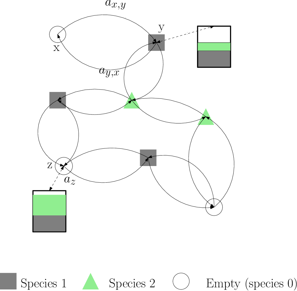
Refer to caption
Figure 2: Hard-core two-species particles on a graph with 8 vertices and 2 reservoirs. Grey squares identify the species 1, green triangles the species 2, and white circles the empty state. The reservoirs are represented by rectangles, where the interior colours denote the density of species.

2.1 Process definition

On the graph G=(V,E)G=(V,E), we consider the Markov process {η​(t);t≥0}\{\eta(t);t\geq 0\} with state space ={0,1,2,…,n}V\Omega=\{0,1,2,\ldots,n\}^{V}. A configuration of the process is denoted by η=(ηx)x∈V\eta=\left(\eta_{x}\right)_{x\in V}, where each component can take the values ηx∈{0,1,…,n}\eta_{x}\in\{0,1,...,n\} and where ηx=α\eta_{x}=\alpha means the presence of the species α\alpha at the site xx. We recall that ηx=0\eta_{x}=0 is interpreted as an empty site. The process is defined by the generator ℒ\mathcal{L} working on functions f: →Rf:\Omega\to\mathbb{R} as

(ℒ​f)​(η)=(ℒe​d​g​e​f)​(η)+(ℒs​i​t​e​f)​(η),(\mathcal{L}f)(\eta)=(\mathcal{L}_{edge}f)(\eta)+(\mathcal{L}_{site}f)(\eta), (10)

where

(ℒe​d​g​e​f)​(η)=∑(x,y)∈Eax,y⋅(ℒx,y​f)​(η)(\mathcal{L}_{edge}f)(\eta)=\sumop\displaylimits_{(x,y)\in E}a_{x,y}\cdot({\mathcal{L}}_{x,y}f)(\eta)

and

(ℒs​i​t​e​f)​(η)=∑x∈Vax⋅(ℒx​f)​(η)(\mathcal{L}_{site}f)(\eta)=\sumop\displaylimits_{x\in V}a_{x}\cdot(\mathcal{L}_{x}f)(\eta)

We shall explain the two generators ℒe​d​g​e\mathcal{L}_{edge} and ℒs​i​t​e\mathcal{L}_{site} in the following subsections.

2.1.1 The edge generator

We introduce the (n+1)2×(n+1)2(n+1)^{2}\times(n+1)^{2} matrix �\Gamma whose elements are rates of transition for the particle jumps on each edge. More precisely, we denote by �γ​δα​β\Gamma_{\gamma\delta}^{\alpha\beta} the rate to change the configuration η\eta with ηx=γ,ηy=δ\eta_{x}=\gamma,\eta_{y}=\delta to the configuration η′\eta^{\prime} with ηx′=α,ηy′=β\eta^{\prime}_{x}=\alpha,\eta^{\prime}_{y}=\beta, while ηz′=ηz\eta^{\prime}_{z}=\eta_{z} for all z,x,yz\neq x,y. Thus, the single-edge generator is given by

ℒx,y​f​(η1,…,γ,…,δ,…,ηN)\displaystyle\mathcal{L}_{x,y}f(\eta_{1},\ldots,\gamma,\ldots,\delta,\ldots,\eta_{N})
=∑α,β=0n�γ​δα​β​[f⁡(η1,…,α,…,β,…,ηN)−f⁡(η1,…,γ,…,δ,…,ηN)]\displaystyle=\sumop\displaylimits_{\alpha,\beta=0}^{n}\Gamma_{\gamma\delta}^{\alpha\beta}\left[f(\eta_{1},\ldots,\alpha,\ldots,\beta,\ldots,\eta_{N})-f(\eta_{1},\ldots,\gamma,\ldots,\delta,\ldots,\eta_{N})\right] (11)

where

�γ​δα​β≥0\displaystyle\Gamma_{\gamma\delta}^{\alpha\beta}\geq 0\qquad if(α,β),(γ,δ)\displaystyle\text{if}\quad(\alpha,\beta)\neq(\gamma,\delta)
∑(γ,δ)∈{0,1,2,…,n}2:(γ​δ),(α,β)�γ​δα​β=−�α​βα​β\displaystyle\sumop\displaylimits_{(\gamma,\delta)\in\{0,1,2,\ldots,n\}^{2}\;:\;(\gamma\delta)\neq(\alpha,\beta)}\Gamma_{\gamma\delta}^{\alpha\beta}=-\Gamma_{\alpha\beta}^{\alpha\beta}\quad ∀(α,β)∈{0,1,2,…,n}2.\displaystyle\forall(\alpha,\beta)\in\{0,1,2,\ldots,n\}^{2}\,.

2.1.2 The site generator

Having in mind that the site generator will describe a ‘boundary’ driving leading the system to a non-equilibrium steady state, we assume that on each site there is a process which injects and removes particles at a rate which is space-dependent. Thus, for each vertex x∈Vx\in V, we introduce the (n+1)×(n+1)(n+1)\times(n+1) matrix W⁡(x)W(x) whose elements are rates of transitions on that vertex. More precisely, we denote by Wγα​(x)W_{\gamma}^{\alpha}(x) the rate to change the configuration η\eta with ηx=γ\eta_{x}=\gamma into the configuration η′\eta^{\prime} with ηx′=α\eta^{\prime}_{x}=\alpha, while ηz′=ηz\eta^{\prime}_{z}=\eta_{z} for all z,xz\neq x. The single-vertex generator is given by

ℒx​f​(η1,…,γ,…,ηN)=\displaystyle\mathcal{L}_{x}f(\eta_{1},\ldots,\gamma,\ldots,\eta_{N})= ∑α=0nWγα(x)[f(η1,…,α,….,ηN)−f(η1,…,γ,…,ηN)]\displaystyle\sumop\displaylimits_{\alpha=0}^{n}W_{\gamma}^{\alpha}(x)\left[f(\eta_{1},\ldots,\alpha,\ldots.,\eta_{N})-f(\eta_{1},\ldots,\gamma,\ldots,\eta_{N})\right] (12)

where

Wγα​(x)≥0\displaystyle W_{\gamma}^{\alpha}(x)\geq 0\quad ifα,γ\displaystyle\text{if}\quad\alpha\neq\gamma
∑γ∈{0,1,2,…,n}:γ,αWγα(x)=−Wαα(x)\displaystyle\sumop\displaylimits_{\gamma\in\{0,1,2,\ldots,n\}:\gamma\neq\alpha}W_{\gamma}^{\alpha}(x)=-W_{\alpha}^{\alpha}(x)\quad ∀α∈{0,1,2,…,n}.\displaystyle\forall\alpha\in\{0,1,2,\ldots,n\}\,.

2.2 Comparison to other processes

Here, we discuss the relation of the general dynamics described above to some multi-species processes considered in the past literature (we consider here the case of homogeneous conductances and inhomogeneities ax,y=ax=1a_{x,y}=a_{x}=1). We shall mostly limit the discussion to symmetric systems (for asymmetric models there is also a large literature, see for instance [10] and references therein). In most cases, previous analyses have been restricted to a regular lattice or a one-dimensional chain.

  • •

    General multi-species models. The edge dynamics of the reaction-diffusion particle system in Section 2.1 has been considered on a d-dimensional lattice in [21] for the case n=1n=1 species and in [22] for the case of an arbitrary number of species. In those papers, sufficient conditions on the rates �γ​δα​β\Gamma_{\gamma\delta}^{\alpha\beta} to guarantee the existence of dual process have been identified.

  • •

    Multi-species exclusion processes. The edge dynamics of multi-species simple symmetric exclusion processes on a d-dimensional lattice, with at most one-particle per site, has been considered in [25]. It corresponds to the model of Section 2.1 with �0​αα​0=�α​00​α​,0\Gamma_{0\alpha}^{\alpha 0}=\Gamma_{\alpha 0}^{0\alpha}\neq 0 for all α=0,1,…,n\alpha=0,1,\ldots,n, while all other off-diagonal elements of the matrix �\Gamma vanish, as well as the elements of the matrices W⁡(x)W(x). For this model, the hierarchy of equations for the correlations does not close, and the hydrodynamic limit has been shown in [25] to be given by two coupled non-linear heat equations. An open boundary version of the model with simple symmetric exclusion dynamic in the bulk has been presented in [26]. It corresponds to the model of Section 2.1 with �b​00​b=�0​bb​0=Db\Gamma_{b0}^{0b}=\Gamma_{0b}^{b0}=D_{b} and with boundary rates W0b​(1)=αb,Wb0=γb,W0b​(N)=βb,Wb0​(N)=δbW^{b}_{0}(1)=\alpha_{b},W_{b}^{0}=\gamma_{b},W_{0}^{b}(N)=\beta_{b},W_{b}^{0}(N)=\delta_{b} (here bb labels the species). All the other off-diagonal elements �\Gamma and W⁡(z)W(z) vanish.

  • •

    Multi-species stirring process. In the stirring process [27, 28], every couple of types is exchanged in position with the same rate, which can be taken equal to 1 without loss of generality. Thus, the bulk dynamics of the stirring process corresponds to the case �γ​δδ​γ=1\Gamma_{\gamma\delta}^{\delta\gamma}=1 for all γ,δ=0,1,…,n\gamma,\delta=0,1,\ldots,n, while all other off-diagonal elements of the matrix �\Gamma vanish. The hydrodynamic limit of the stirring process on a lattice is given by nn independent diffusions, i.e. the generalization of (8) to nn types. The multi-species stirring process on a chain with boundary driving has been studied in [29] with the choice Wγb​(1)=αbW_{\gamma}^{b}(1)=\alpha_{b} and Wγb​(N)=βbW_{\gamma}^{b}(N)=\beta_{b}. With this particular choice of the boundary rates the model is solvable and correlation functions in the non equilibrium steady state have been computed using the matrix product ansatz.

  • •

    Multi-species switching process: A different set-up for multi-species particle systems has been recently proposed in [8, 30]. One considers nn “piled” copies of the graph GG, each with its own single-type dynamics. The possibility of changing type is described by a switching rate between layers. This set-up eliminates the constraint of one particle per site, in the sense that the projection of the dynamics on the columns of the piled graph allows the presence of several particle of different types on the same “base” site. In the case where each layer is a one-dimensional chain and two-layers are considered, the hydrodynamic limit has been shown to be given by the “weakly” coupled reaction diffusion equation (9). When boundary reservoirs are added, global uphill diffusion and boundary layers are possible [8].

3 Evolution equations for the average occupation

For the model introduced in Section 2.1, we define the average of the occupation variable of each species ζ∈{0,1,…,n}\zeta\in\{0,1,\ldots,n\} at time t≥0t\geq 0 and at the vertex z∈Vz\in V

μz(ζ)​(t)=E⁡[𝟙{ℐzζ}​(η​(t))].\mu_{z}^{(\zeta)}(t)=\mathbb{E}\left[\mathbbm{1}_{\{\mathcal{I}^{\zeta}_{z}\}}(\eta(t))\right]. (13)

Similarly, we consider the time-dependent correlations between species ζ,ζ′∈{0,1,…,n}\zeta,\zeta^{\prime}\in\{0,1,\ldots,n\} at points z,z′∈Vz,z^{\prime}\in V

cz,z′(ζ,ζ′)​(t)=E⁡[𝟙{ℐzζ}​(η​(t))​𝟙{ℐz′ζ′}​(η​(t))].c_{z,z^{\prime}}^{(\zeta,\zeta^{\prime})}(t)=\mathbb{E}\left[\mathbbm{1}_{\{\mathcal{I}^{\zeta}_{z}\}}(\eta(t))\mathbbm{1}_{\{\mathcal{I}^{\zeta^{\prime}}_{z^{\prime}}\}}(\eta(t))\right]. (14)

Here ℐzζ={η∈ :ηz=ζ}\mathcal{I}_{z}^{\zeta}=\{\eta\in\Omega\,:\;\eta_{z}=\zeta\} and 𝟙ℐ\mathbbm{1}_{\mathcal{I}} denotes the indicator function of the set ℐ\mathcal{I}. The notation E⁡[f⁡(η​(t))]=∫ν0​(𝑑η)​Eη​[f⁡(η​(t))]\mathbb{E}\left[f(\eta(t))\right]=\intop\nolimits\nu_{0}(d\eta)\mathbb{E}_{\eta}\left[f(\eta(t))\right] denotes the expectation in the process {η​(t)}t≥0\{\eta(t)\}_{t\geq 0} started from the initial measure ν0\nu_{0}. The evolution equation of the density of the ζ\zeta-species can be obtained by acting with the generator. We have

d​E​[𝟙{ℐzζ}​(η​(t))]d​t=E⁡[(ℒ​𝟙{ℐzζ})​(η​(t))].\frac{d\mathbb{E}\left[\mathbbm{1}_{\{\mathcal{I}^{\zeta}_{z}\}}(\eta(t))\right]}{dt}=\mathbb{E}\left[\left(\mathcal{L}\mathbbm{1}_{\{\mathcal{I}^{\zeta}_{z}\}}\right)(\eta(t))\right]. (15)

In the following section we evaluate the right hand side of this equation by considering first edge contributions and then site contributions.

3.1 Action of ℒx,y\mathcal{L}_{x,y}

If z<{x,y}z\notin\{x,y\} then obviously (ℒx,y​𝟙{ℐzζ})​(η)=0\left(\mathcal{L}_{x,y}\mathbbm{1}_{\{\mathcal{I}_{z}^{\zeta}\}}\right)(\eta)=0. Otherwise, recalling that the graph GG is directed and the notation of [22], we have the following: when we fix z=xz=x then

(ℒz,y​𝟙{ℐzζ})​(η)=A1ζ+∑δ=1nF+1ζ​δ​𝟙{ℐyδ}​(η)+∑γ=1nB1ζ​γ​𝟙{ℐzγ}​(η)+∑γ,δ=1nG+1ζ​γ​δ​𝟙{ℐyγ}​(η)​𝟙{ℐzδ}​(η)\left(\mathcal{L}_{z,y}\mathbbm{1}_{\{\mathcal{I}_{z}^{\zeta}\}}\right)(\eta)=A^{\zeta}_{1}+\sumop\displaylimits_{\delta=1}^{n}F_{+1}^{\zeta\delta}\mathbbm{1}_{\{\mathcal{I}_{y}^{\delta}\}}(\eta)+\sumop\displaylimits_{\gamma=1}^{n}B_{1}^{\zeta\gamma}\mathbbm{1}_{\{\mathcal{I}_{z}^{\gamma}\}}(\eta)+\sumop\displaylimits_{\gamma,\delta=1}^{n}G_{+1}^{\zeta\gamma\delta}\mathbbm{1}_{\{\mathcal{I}_{y}^{\gamma}\}}(\eta)\mathbbm{1}_{\{\mathcal{I}_{z}^{\delta}\}}(\eta) (16)

and when we fix z=yz=y then

(ℒx,z​𝟙{ℐzζ})​(η)=A2ζ+∑γ=1nF−1ζ​γ​𝟙{ℐxγ}​(η)+∑δ=1nC2ζ​δ​𝟙{ℐzδ}​(η)+∑γ,δ=1nG−1ζ​γ​δ​𝟙{ℐzγ}​(η)​𝟙{ℐxδ}​(η)\left(\mathcal{L}_{x,z}\mathbbm{1}_{\{\mathcal{I}_{z}^{\zeta}\}}\right)(\eta)=A^{\zeta}_{2}+\sumop\displaylimits_{\gamma=1}^{n}F_{-1}^{\zeta\gamma}\mathbbm{1}_{\{\mathcal{I}_{x}^{\gamma}\}}(\eta)+\sumop\displaylimits_{\delta=1}^{n}C_{2}^{\zeta\delta}\mathbbm{1}_{\{\mathcal{I}_{z}^{\delta}\}}(\eta)+\sumop\displaylimits_{\gamma,\delta=1}^{n}G_{-1}^{\zeta\gamma\delta}\mathbbm{1}_{\{\mathcal{I}_{z}^{\gamma}\}}(\eta)\mathbbm{1}_{\{\mathcal{I}_{x}^{\delta}\}}(\eta) (17)

where the constants are defined as follows:

  1. 1.

    zero-order terms:

    A1ζ\displaystyle A^{\zeta}_{1} =∑β=0n�00ζ​βA2ζ=∑β=0n�00β​ζ\displaystyle=\sumop\displaylimits_{\beta=0}^{n}\Gamma_{00}^{\zeta\beta}\qquad\qquad A^{\zeta}_{2}=\sumop\displaylimits_{\beta=0}^{n}\Gamma_{00}^{\beta\zeta}
  2. 2.

    first-order terms:

    B1ζ​γ\displaystyle B_{1}^{\zeta\gamma} ={∑β=0n(�γ​0ζ​β−�00ζ​β)if ​ζ,γ−∑β=0n(∑ζ′=0:ζ′,ζn�ζ​0ζ′β+�00ζ​β)if ζ=γ\displaystyle=\begin{cases}\sumop\displaylimits_{\beta=0}^{n}(\Gamma_{\gamma 0}^{\zeta\beta}-\Gamma_{00}^{\zeta\beta})\;\;\;\;\quad\qquad\qquad\quad\text{if }\;\zeta\neq\gamma\\ -\sumop\displaylimits_{\beta=0}^{n}\left(\sumop\displaylimits_{\zeta^{{}^{\prime}}=0\;:\;\zeta^{{}^{\prime}}\neq\zeta}^{n}\Gamma_{\zeta 0}^{\zeta^{{}^{\prime}}\beta}+\Gamma_{00}^{\zeta\beta}\right)\;\;\;\;\;\text{if }\;\zeta=\gamma\\ \end{cases}
    C2ζ​δ\displaystyle C_{2}^{\zeta\delta} ={∑β=0n(�0​δβ​ζ−�00β​ζ)if​ζ,δ−∑β=0n(∑ζ′=0:ζ′,ζn�0​ζβζ′+�00β​ζ)ifζ=δ\displaystyle=\begin{cases}\sumop\displaylimits_{\beta=0}^{n}(\Gamma^{\beta\zeta}_{0\delta}-\Gamma_{00}^{\beta\zeta})\qquad\qquad\qquad\;\;\;\;\;\text{if}\;\zeta\neq\delta\\ -\sumop\displaylimits_{\beta=0}^{n}\left(\sumop\displaylimits_{\zeta^{{}^{\prime}}=0\;:\;\zeta^{{}^{\prime}}\neq\zeta}^{n}\Gamma_{0\zeta}^{\beta\zeta^{{}^{\prime}}}+\Gamma_{00}^{\beta\zeta}\right)\;\;\;\;\;\text{if}\;\zeta=\delta\\ \end{cases}
    F−1ζ​γ\displaystyle F_{-1}^{\zeta\gamma} =B2ζ​γ=∑β=0n(�γ​0β​ζ−�00β​ζ)\displaystyle=B_{2}^{\zeta\gamma}=\sumop\displaylimits_{\beta=0}^{n}(\Gamma_{\gamma 0}^{\beta\zeta}-\Gamma_{00}^{\beta\zeta})
    F+1ζ​δ\displaystyle F_{+1}^{\zeta\delta} =C1ζ​δ=∑β=0n(�0​δζ​β−�00ζ​β)\displaystyle=C_{1}^{\zeta\delta}=\sumop\displaylimits_{\beta=0}^{n}(\Gamma_{0\delta}^{\zeta\beta}-\Gamma_{00}^{\zeta\beta})
  3. 3.

    second-order terms:

    G+1ζ​γ​δ\displaystyle G_{+1}^{\zeta\gamma\delta} =D1ζ,γ,δ={∑β=0n(�γ​δζ​β−�γ​0ζ​β−�0​δζ​β+�00ζ​β);if ​ζ,γ−∑β=0n(∑ζ′=0:ζ′,ζn�ζ​δζ′β+�0​δζ​β)+∑β=0n(∑ζ′=0:ζ′,ζn�ζ​0ζ′β+�00ζ​β)if ζ=γ\displaystyle=D_{1}^{\zeta,\gamma,\delta}=\begin{cases}\sumop\displaylimits_{\beta=0}^{n}(\Gamma_{\gamma\delta}^{\zeta\beta}-\Gamma_{\gamma 0}^{\zeta\beta}-\Gamma_{0\delta}^{\zeta\beta}+\Gamma_{00}^{\zeta\beta});\;\;\;\;\qquad\qquad\qquad\qquad\qquad\qquad\qquad\text{if }\;\zeta\neq\gamma\\ -\sumop\displaylimits_{\beta=0}^{n}\left(\sumop\displaylimits_{\zeta^{{}^{\prime}}=0\;:\;\zeta^{{}^{\prime}}\neq\zeta}^{n}\Gamma_{\zeta\delta}^{\zeta^{{}^{\prime}}\beta}+\Gamma_{0\delta}^{\zeta\beta}\right)+\sumop\displaylimits_{\beta=0}^{n}\left(\sumop\displaylimits_{\zeta^{{}^{\prime}}=0\;:\;\zeta^{{}^{\prime}}\neq\zeta}^{n}\Gamma_{\zeta 0}^{\zeta^{{}^{\prime}}\beta}+\Gamma_{00}^{\zeta\beta}\right)\;\;\;\;\text{if }\;\zeta=\gamma\end{cases}
    G−1ζ​γ​δ\displaystyle G_{-1}^{\zeta\gamma\delta} =D2ζ,γ,δ={∑β=0n(�γ​δβ​ζ−�γ​0β​ζ−�0​δβ​ζ+�00β​ζ)if ​ζ,δ−∑β=0n(∑ζ′=0:ζ′,ζn�γ​ζβζ′+�γ​0β​ζ)+∑β=0n(∑ζ′=0:ζ′,ζn�0​ζβζ′+�00β​ζ)if ζ=δ\displaystyle=D_{2}^{\zeta,\gamma,\delta}=\begin{cases}\sumop\displaylimits_{\beta=0}^{n}(\Gamma_{\gamma\delta}^{\beta\zeta}-\Gamma_{\gamma 0}^{\beta\zeta}-\Gamma_{0\delta}^{\beta\zeta}+\Gamma_{00}^{\beta\zeta})\;\;\;\;\qquad\qquad\qquad\qquad\qquad\qquad\qquad\text{if }\;\zeta\neq\delta\\ -\sumop\displaylimits_{\beta=0}^{n}\left(\sumop\displaylimits_{\zeta^{{}^{\prime}}=0\;:\;\zeta^{{}^{\prime}}\neq\zeta}^{n}\Gamma_{\gamma\zeta}^{\beta\zeta^{{}^{\prime}}}+\Gamma_{\gamma 0}^{\beta\zeta}\right)+\sumop\displaylimits_{\beta=0}^{n}\left(\sumop\displaylimits_{\zeta^{{}^{\prime}}=0\;:\;\zeta^{{}^{\prime}}\neq\zeta}^{n}\Gamma_{0\zeta}^{\beta\zeta^{{}^{\prime}}}+\Gamma_{00}^{\beta\zeta}\right)\;\;\;\;\;\text{if }\;\zeta=\delta\end{cases}

3.2 Action of ℒx\mathcal{L}_{x}

If z,xz\neq x then obviously (ℒx​𝟙{ℐzζ})​(η)=0\left(\mathcal{L}_{x}\mathbbm{1}_{\{\mathcal{I}_{z}^{\zeta}\}}\right)(\eta)=0. Otherwise

(ℒz​𝟙{ℐzζ})​(η)=Aζ​(z)+∑β=1nFζ​β​(z)​𝟙{ℐzβ}​(η)\left(\mathcal{L}_{z}\mathbbm{1}_{\{\mathcal{I}_{z}^{\zeta}\}}\right)(\eta)=A^{\zeta}(z)+\sumop\displaylimits_{\beta=1}^{n}F^{\zeta\beta}(z)\mathbbm{1}_{\{\mathcal{I}_{z}^{\beta}\}}(\eta) (18)

where now the constants are defined as:

  1. 1.

    zero-order term:

    Aζ​(z)\displaystyle A^{\zeta}(z) =W0ζ​(z)\displaystyle=W_{0}^{\zeta}(z)
  2. 2.

    first-order term:

    Fζ​β(z)={Wβζ​(z)−W0ζ​(z)if ​ζ,β−∑ζ′=0:ζ′,ζnWζζ′(z)−W0ζ(z)if ζ=β.F^{\zeta\beta}(z)=\begin{cases}W_{\beta}^{\zeta}(z)-W_{0}^{\zeta}(z)\qquad\qquad\qquad\qquad\;\;\;\text{if }\;\zeta\neq\beta\\ -\sumop\displaylimits_{\zeta^{{}^{\prime}}=0\;:\;\zeta^{{}^{\prime}}\neq\zeta}^{n}W_{\zeta}^{\zeta^{{}^{\prime}}}(z)-W_{0}^{\zeta}(z)\qquad\text{if }\;\zeta=\beta\end{cases}.

3.3 Action of ℒ\mathcal{L}

We now collect the results of the previous sections. We may write

(ℒ​𝟙{ℐzζ})​(η)\displaystyle\left(\mathcal{L}\mathbbm{1}_{\{\mathcal{I}_{z}^{\zeta}\}}\right)(\eta) =\displaystyle= ∑x,y:(x,y)∈Eax,y(ℒx,y𝟙{ℐzζ})(η)+∑xax(ℒx𝟙{ℐzζ})(η)\displaystyle\sumop\displaylimits_{x,y\;:\;(x,y)\in E}a_{x,y}\left(\mathcal{L}_{x,y}\mathbbm{1}_{\{\mathcal{I}_{z}^{\zeta}\}}\right)(\eta)+\sumop\displaylimits_{x}a_{x}\left(\mathcal{L}_{x}\mathbbm{1}_{\{\mathcal{I}_{z}^{\zeta}\}}\right)(\eta)
=\displaystyle= ∑y:(z,y)∈Eaz,y(ℒz,y𝟙{ℐzζ})(η)+∑x:(x,z)∈Eax,z(ℒx,z𝟙{ℐzζ})(η)+az(ℒz𝟙{ℐzζ})(η).\displaystyle\sumop\displaylimits_{y\;:\;(z,y)\in E}a_{z,y}\left(\mathcal{L}_{z,y}\mathbbm{1}_{\{\mathcal{I}_{z}^{\zeta}\}}\right)(\eta)+\sumop\displaylimits_{x\;:\;(x,z)\in E}a_{x,z}\left(\mathcal{L}_{x,z}\mathbbm{1}_{\{\mathcal{I}_{z}^{\zeta}\}}\right)(\eta)+a_{z}\left(\mathcal{L}_{z}\mathbbm{1}_{\{\mathcal{I}_{z}^{\zeta}\}}\right)(\eta).

Substituting (16), (17), (18) in the above expression we obtain

(ℒ​𝟙{ℐzζ})​(η)\displaystyle\left(\mathcal{L}\mathbbm{1}_{\{\mathcal{I}_{z}^{\zeta}\}}\right)(\eta) =\displaystyle= ∑y:(z,y)∈Eaz,y(A1ζ+∑δ=1nF+1ζ​δ𝟙{ℐyδ}(η)+∑γ=1nB1ζ​γ𝟙{ℐzγ}(η)+∑γ,δ=1nG+1ζ​γ​δ𝟙{ℐyγ}(η)𝟙{ℐzδ}(η))\displaystyle\sumop\displaylimits_{y\;:\;(z,y)\in E}a_{z,y}\left(A^{\zeta}_{1}+\sumop\displaylimits_{\delta=1}^{n}F_{+1}^{\zeta\delta}\mathbbm{1}_{\{\mathcal{I}_{y}^{\delta}\}}(\eta)+\sumop\displaylimits_{\gamma=1}^{n}B_{1}^{\zeta\gamma}\mathbbm{1}_{\{\mathcal{I}_{z}^{\gamma}\}}(\eta)+\sumop\displaylimits_{\gamma,\delta=1}^{n}G_{+1}^{\zeta\gamma\delta}\mathbbm{1}_{\{\mathcal{I}_{y}^{\gamma}\}}(\eta)\mathbbm{1}_{\{\mathcal{I}_{z}^{\delta}\}}(\eta)\right) (19)
+\displaystyle+ ∑x:(x,z)∈Eax,z(A2ζ+∑γ=1nF−1ζ​γ𝟙{ℐxγ}(η)+∑δ=1nC2ζ​δ𝟙{ℐzδ}(η)+∑γ,δ=1nG−1ζ​γ​δ𝟙{ℐzγ}(η)𝟙{ℐxδ}(η))\displaystyle\sumop\displaylimits_{x\;:\;(x,z)\in E}a_{x,z}\left(A^{\zeta}_{2}+\sumop\displaylimits_{\gamma=1}^{n}F_{-1}^{\zeta\gamma}\mathbbm{1}_{\{\mathcal{I}_{x}^{\gamma}\}}(\eta)+\sumop\displaylimits_{\delta=1}^{n}C_{2}^{\zeta\delta}\mathbbm{1}_{\{\mathcal{I}_{z}^{\delta}\}}(\eta)+\sumop\displaylimits_{\gamma,\delta=1}^{n}G_{-1}^{\zeta\gamma\delta}\mathbbm{1}_{\{\mathcal{I}_{z}^{\gamma}\}}(\eta)\mathbbm{1}_{\{\mathcal{I}_{x}^{\delta}\}}(\eta)\right)
+\displaystyle+ az​(Aζ​(z)+∑β=1nFζ​β​(z)​𝟙{ℐzβ}​(η)).\displaystyle a_{z}\left(A^{\zeta}(z)+\sumop\displaylimits_{\beta=1}^{n}F^{\zeta\beta}(z)\mathbbm{1}_{\{\mathcal{I}_{z}^{\beta}\}}(\eta)\right).

3.4 Evolution equations

Using equation (19) for the right hand side of (15) we obtain the evolution equation for the average occupation. Recalling the notation in (13) and (14) (for the sake of space we do not write the explicit tt-dependence) we arrive to

dd​t​μz(ζ)\displaystyle\frac{d}{dt}\mu_{z}^{(\zeta)} =\displaystyle= ∑y:(z,y)∈Eaz,y(A1ζ+∑δ=1nF+1ζ​δμy(δ)+∑γ=1nB1ζ​γμz(γ)+∑γ,δ=1nG+1ζ​γ​δcy,z(γ,δ))\displaystyle\sumop\displaylimits_{y\;:\;(z,y)\in E}a_{z,y}\left(A^{\zeta}_{1}+\sumop\displaylimits_{\delta=1}^{n}F_{+1}^{\zeta\delta}\;\mu_{y}^{(\delta)}+\sumop\displaylimits_{\gamma=1}^{n}B_{1}^{\zeta\gamma}\;\mu_{z}^{(\gamma)}+\sumop\displaylimits_{\gamma,\delta=1}^{n}G_{+1}^{\zeta\gamma\delta}\;c_{y,z}^{(\gamma,\delta)}\right) (20)
+\displaystyle+ ∑x:(x,z)∈Eax,z(A2ζ+∑γ=1nF−1ζ​γμx(γ)+∑δ=1nC2ζ​δμz(δ)+∑γ,δ=1nG−1ζ​γ​δcz,x(γ,δ))\displaystyle\sumop\displaylimits_{x\;:\;(x,z)\in E}a_{x,z}\left(A^{\zeta}_{2}+\sumop\displaylimits_{\gamma=1}^{n}F_{-1}^{\zeta\gamma}\;\mu_{x}^{(\gamma)}+\sumop\displaylimits_{\delta=1}^{n}C_{2}^{\zeta\delta}\;\mu_{z}^{(\delta)}+\sumop\displaylimits_{\gamma,\delta=1}^{n}G_{-1}^{\zeta\gamma\delta}\;c_{z,x}^{(\gamma,\delta)}\right)
+\displaystyle+ az​(Aζ​(z)+∑β=1nFζ​β​(z)​μz(β)).\displaystyle a_{z}\left(A^{\zeta}(z)+\sumop\displaylimits_{\beta=1}^{n}F^{\zeta\beta}(z)\;\mu_{z}^{(\beta)}\right).

We notice that the equations for the time-dependent averages μz(ζ)​(t)\mu_{z}^{(\zeta)}(t) are not closed, as they involve the correlations cz,z′(ζ,ζ′)​(t)c_{z,z^{\prime}}^{(\zeta,\zeta^{\prime})}(t).

Remark 3.1 (The process on the lattice)

The generator (10) is an generalization of the lattice generator studied in [22] to a general graph with the addition of open boundaries. Indeed, take as a special graph the dd-dimensional regular lattice Zd\mathbb{Z}^{d} and ignore the boundaries. Then, calling e(k)e^{(k)} the unit vector in the kt​hk^{th} direction (k=1,…,dk=1,\ldots,d) and defining

Eζ=A1ζ+A2ζF0ζ​β=C2ζ​β+B1ζ​β\begin{split}E^{\zeta}=A^{\zeta}_{1}+A^{\zeta}_{2}\\ F_{0}^{\zeta\beta}=C_{2}^{\zeta\beta}+B_{1}^{\zeta\beta}\end{split} (21)

equation (19) becomes

(ℒ𝟙{ℐzζ})(η)=∑k=1d{Eζ+∑β=1n∑j=−1+1Fjζ​β𝟙{ℐz+j​e(k)β}(η)+∑β,β′=1n∑j=±1Gjζββ′𝟙{ℐz+j​e(k)β}(η)𝟙{ℐzβ′}(η)}\begin{split}\left(\mathcal{L}\mathbbm{1}_{\{\mathcal{I}_{z}^{\zeta}\}}\right)(\eta)=\sumop\displaylimits_{k=1}^{d}\left\{E^{\zeta}+\sumop\displaylimits_{\beta=1}^{n}\sumop\displaylimits_{j=-1}^{+1}F_{j}^{\zeta\beta}\mathbbm{1}_{\{\mathcal{I}_{z+je^{(k)}}^{\beta}\}}(\eta)+\sumop\displaylimits_{\beta,\beta^{{}^{\prime}}=1}^{n}\sumop\displaylimits_{j=\pm 1}G_{j}^{\zeta\beta\beta^{{}^{\prime}}}\mathbbm{1}_{\{\mathcal{I}_{z+je^{(k)}}^{\beta}\}}(\eta)\mathbbm{1}_{\{\mathcal{I}_{z}^{\beta^{{}^{\prime}}}\}}(\eta)\right\}\end{split} (22)

which is equation (3.12)(3.12) in [22].

4 Boundary-driven chains with linear reaction-diffusion

In this and the following sections we specialize to the case with only two species, labelled by 11 and 22. Furthermore, we specialize to the one-dimensional geometry by considering a undirected linear chain.

More precisely, the graph has NN vertices labelled by {1,2,…,N}\{1,2,\ldots,N\} with a distinguish role of the sites {1,N}\{1,N\}which model two reservoirs. The interaction is of nearest neighbor type, i.e.

ax,y={1if|x−y|=10otherwiseax={1ifx∈{1,N}0otherwisea_{x,y}=\begin{cases}1\qquad\text{if}\quad|x-y|=1\\ 0\qquad\text{otherwise}\end{cases}\qquad\qquad a_{x}=\begin{cases}1\qquad\text{if}\quad x\in\{1,N\}\\ 0\qquad\text{otherwise}\end{cases}

It is convenient to call the sites {2,…,N−1}\{2,\ldots,N-1\} as “bulk” and the two end sites {1,N}\{1,N\} as “boundary”. The generator of the process thus reads as:

ℒ=ℒ1+∑z=1N−1ℒz,z+1+ℒN\mathcal{L}=\mathcal{L}_{1}+\sumop\displaylimits_{z=1}^{N-1}\mathcal{L}_{z,z+1}+\mathcal{L}_{N} (23)

We specialize the result of Eq. (20) to the boundary-driven chain. Introducing ∀ζ,β=1,2\forall\zeta,\beta=1,2:

F0ζ​β=B1ζ​β+C2ζ​β\displaystyle F_{0}^{\zeta\beta}=B_{1}^{\zeta\beta}+C_{2}^{\zeta\beta}\quad Eζ=A1ζ+A2ζ\displaystyle E^{\zeta}=A_{1}^{\zeta}+A_{2}^{\zeta}
ALζ=Aζ​(1)\displaystyle A_{L}^{\zeta}=A^{\zeta}(1)\quad ARζ=Aζ​(N)\displaystyle A_{R}^{\zeta}=A^{\zeta}(N)
FLζ​β=Fζ​β​(1)\displaystyle F^{\zeta\beta}_{L}=F^{\zeta\beta}(1)\quad FRζ​β=Fζ​β​(N)\displaystyle F^{\zeta\beta}_{R}=F^{\zeta\beta}(N)

the evolution equations for the densities of the two species at site z∈{1,2,…,N}z\in\{1,2,\ldots,N\} are given by:

dd​t​μ1(ζ)=ALζ+A1ζ+∑β=12((B1ζ​β+FLζ​β)​μ1(β)+F+1ζ​β​μ2(β))+∑β,β′=12G+1ζββ′c1,2(β,β′)\begin{split}\frac{d}{dt}\mu_{1}^{(\zeta)}&=A_{L}^{\zeta}+A_{1}^{\zeta}+\sumop\displaylimits_{\beta=1}^{2}\left(\left(B_{1}^{\zeta\beta}+F_{L}^{\zeta\beta}\right)\mu_{1}^{(\beta)}+F_{+1}^{\zeta\beta}\mu_{2}^{(\beta)}\right)\qquad\qquad\qquad\qquad\qquad\qquad\qquad\\ &+\sumop\displaylimits_{\beta,\beta^{{}^{\prime}}=1}^{2}G_{+1}^{\zeta\beta\beta^{{}^{\prime}}}c_{1,2}^{(\beta,\beta^{{}^{\prime}})}\end{split} (24)
dd​t​μz(ζ)=Eζ+∑β=12(F−1ζ​βμz−1(β)+F0ζ​βμz(β)+F+1ζ​βμz+1(β))if z∈{2,…,N−1}+∑β,β′=12(G−1ζββ′cz−1,z(β,β′)+G+1ζββ′cz,z+1(β,β′)}\begin{split}\frac{d}{dt}\mu_{z}^{(\zeta)}&=E^{\zeta}+\sumop\displaylimits_{\beta=1}^{2}\left(F_{-1}^{\zeta\beta}\mu_{z-1}^{(\beta)}+F_{0}^{\zeta\beta}\mu_{z}^{(\beta)}+F_{+1}^{\zeta\beta}\mu_{z+1}^{(\beta)}\right)\qquad\qquad\qquad\text{if }z\in\{2,\ldots,N-1\}\qquad\\ &+\sumop\displaylimits_{\beta,\beta^{{}^{\prime}}=1}^{2}\left(G_{-1}^{\zeta\beta\beta^{{}^{\prime}}}c_{z-1,z}^{(\beta,\beta^{{}^{\prime}})}+G_{+1}^{\zeta\beta\beta^{{}^{\prime}}}c_{z,z+1}^{(\beta,\beta^{{}^{\prime}})}\right\}\end{split} (25)
dd​t​μN(ζ)=ARζ+A2ζ+∑β=12((C2ζ​β+FRζ​β)​μN(β)+F−1ζ​β​μN−1(β))+∑β,β′=12G−1ζββ′cN−1,N(β,β′)\begin{split}\frac{d}{dt}\mu_{N}^{(\zeta)}&=A_{R}^{\zeta}+A_{2}^{\zeta}+\sumop\displaylimits_{\beta=1}^{2}\left(\left(C_{2}^{\zeta\beta}+F_{R}^{\zeta\beta}\right)\mu_{N}^{(\beta)}+F_{-1}^{\zeta\beta}\mu_{N-1}^{(\beta)}\right)\qquad\qquad\qquad\qquad\qquad\qquad\\ &+\sumop\displaylimits_{\beta,\beta^{{}^{\prime}}=1}^{2}G_{-1}^{\zeta\beta\beta^{{}^{\prime}}}c_{N-1,N}^{(\beta,\beta^{{}^{\prime}})}\end{split} (26)

In the next section, we simplify the evolution equations for the average density by selecting a subclass of processes with closed equations and a linear structure.

4.1 Imposing the matching

One could go further and compute the hierarchy of equations for higher-order correlation function [22]. For general choices of the rate matrices �\Gamma and WW, the equations do not close. In the following, we shall focus on those choices of rates that satisfy the following two requirements:

  1. 1.

    Closure of the correlation equations. This amounts to requiring that the correlation terms in (24), (25), (26) vanish. It is shown in [22] that the vanishing of correlations actually implies closure of the multi-point correlation function at all orders.

  2. 2.

    The average occupations follow the discretization of the reaction diffusion equation. Considering the reaction diffusion system (5), we approximate the laplacians with the central difference operators. We call ρi(α)\rho_{i}^{(\alpha)} the density of species α∈{0,1,2}\alpha\in\{0,1,2\} at vertex i∈{1,…,N}i\in\{1,\ldots,N\} with the constraint ρi(0)+ρi(1)+ρi(2)=1\rho_{i}^{(0)}+\rho_{i}^{(1)}+\rho_{i}^{(2)}=1. Furthermore we fix the densities at the left end (vertex 1) to the values of ρL(1)\rho_{L}^{(1)}, ρL(2)\rho_{L}^{(2)} and similarly at the right end (vertex NN) we impose ρR(1)\rho_{R}^{(1)}, ρR(2)\rho_{R}^{(2)}. Then the discretization of the two component reaction diffusion equations (5), reads as

    dd​t​ρ1(1)=σ11​(ρL(1)−2​ρ1(1)+ρ2(1))+σ12​(ρL(2)−2​ρ1(2)+ρ2(2))+�⁡(ρ1(2)−ρ1(1))dd​t​ρ1(2)=σ21​(ρL(1)−2​ρ1(1)+ρ2(1))+σ22​(ρL(2)−2​ρ1(2)+ρ2(2))+�⁡(ρ1(1)−ρ2(2))\begin{split}\frac{d}{dt}\rho_{1}^{(1)}=&\sigma_{11}\left(\rho_{L}^{(1)}-2\rho^{(1)}_{1}+\rho^{(1)}_{2}\right)+\sigma_{12}\left(\rho_{L}^{(2)}-2\rho^{(2)}_{1}+\rho^{(2)}_{2}\right)+\Upsilon\left(\rho^{(2)}_{1}-\rho^{(1)}_{1}\right)\\ \frac{d}{dt}\rho_{1}^{(2)}=&\sigma_{21}\left(\rho_{L}^{(1)}-2\rho^{(1)}_{1}+\rho^{(1)}_{2}\right)+\sigma_{22}\left(\rho_{L}^{(2)}-2\rho^{(2)}_{1}+\rho^{(2)}_{2}\right)+\Upsilon\left(\rho^{(1)}_{1}-\rho^{(2)}_{2}\right)\end{split} (27)
    dd​t​ρz(1)=σ11​(ρz−1(1)−2​ρz(1)+ρz+1(1))+σ12​(ρz−1(2)−2​ρz(2)+ρz+1(2))+�⁡(ρz(2)−ρz(1))dd​t​ρz(2)=σ21​(ρz−1(1)−2​ρz(1)+ρz+1(1))+σ22​(ρz−1(2)−2​ρz(2)+ρz+1(2))+�⁡(ρz(1)−ρz(2))∀z=2,…,N−1\begin{split}\frac{d}{dt}\rho_{z}^{(1)}&=\sigma_{11}\left(\rho^{(1)}_{z-1}-2\rho^{(1)}_{z}+\rho^{(1)}_{z+1}\right)+\sigma_{12}\left(\rho^{(2)}_{z-1}-2\rho^{(2)}_{z}+\rho^{(2)}_{z+1}\right)+\Upsilon\left(\rho^{(2)}_{z}-\rho^{(1)}_{z}\right)\\ \frac{d}{dt}\rho_{z}^{(2)}&=\sigma_{21}\left(\rho^{(1)}_{z-1}-2\rho^{(1)}_{z}+\rho^{(1)}_{z+1}\right)+\sigma_{22}\left(\rho^{(2)}_{z-1}-2\rho^{(2)}_{z}+\rho^{(2)}_{z+1}\right)+\Upsilon\left(\rho^{(1)}_{z}-\rho^{(2)}_{z}\right)\\ &\qquad\qquad\qquad\qquad\qquad\qquad\qquad\qquad\qquad\qquad\qquad\qquad\forall z=2,\ldots,N-1\end{split} (28)
    dd​t​ρN(1)=σ11​(ρN−1(1)−2​ρN(1)+ρR(1))+σ12​(ρN−1(2)−2​ρN(2)+ρR(2))+�⁡(ρN(2)−ρN(1))dd​t​ρN(2)=σ21​(ρN−1(1)−2​ρN(1)+ρR(1))+σ22​(ρN−1(2)−2​ρN(2)+ρR(2))+�⁡(ρN(1)−ρN(2))\begin{split}\frac{d}{dt}\rho_{N}^{(1)}=&\sigma_{11}\left(\rho_{N-1}^{(1)}-2\rho^{(1)}_{N}+\rho^{(1)}_{R}\right)+\sigma_{12}\left(\rho_{N-1}^{(2)}-2\rho^{(2)}_{N}+\rho^{(2)}_{R}\right)+\Upsilon\left(\rho^{(2)}_{N}-\rho^{(1)}_{N}\right)\\ \frac{d}{dt}\rho_{N}^{(2)}=&\sigma_{21}\left(\rho_{N-1}^{(1)}-2\rho^{(1)}_{N}+\rho^{(1)}_{R}\right)+\sigma_{22}\left(\rho_{N-1}^{(2)}-2\rho^{(2)}_{N}+\rho^{(2)}_{R}\right)+\Upsilon\left(\rho^{(1)}_{N}-\rho^{(2)}_{N}\right)\end{split} (29)

    We impose that the evolution equations for the averaged occupations given in (24), (25), (26) do coincide with the discretized reaction-diffusion equations (27), (28), (29).

By imposing the closure condition 1. and the discrete linear reaction-diffusion condition 2. we get the set of equations described below.

Conditions from the bulk.

We first consider equation (25) which we require to have the form of (28). We obtain the following conditions:

  • •

    Closure conditions: equation (28) has no second order terms, thus:

    G+1αββ′=0G−1αββ′=0∀α,β,β′=1,2G_{+1}^{\alpha\beta\beta^{{}^{\prime}}}=0\qquad G_{-1}^{\alpha\beta\beta^{{}^{\prime}}}=0\quad\forall\alpha,\beta,\beta^{{}^{\prime}}=1,2 (30)

    The above requirement leads to 1616 conditions on the transition rates �γ​δα​β\Gamma_{\gamma\delta}^{\alpha\beta}.

  • •

    Laplacian conditions: the one point correlation function should evolve as the coupled discrete Laplacian in (28) with linear reaction. This is accomplished by imposing:

    F−111=F+111=σ11\displaystyle F_{-1}^{11}=F_{+1}^{11}=\sigma_{11} F−112=F+112=σ12\displaystyle F_{-1}^{12}=F_{+1}^{12}=\sigma_{12} F−121=F+121=σ21\displaystyle F_{-1}^{21}=F_{+1}^{21}=\sigma_{21} F−122=F+122=σ22\displaystyle F_{-1}^{22}=F_{+1}^{22}=\sigma_{22}
    F011=−2​σ11−�\displaystyle F_{0}^{11}=-2\sigma_{11}-\Upsilon F012=−2​σ12+�\displaystyle F_{0}^{12}=-2\sigma_{12}+\Upsilon F021=−2​σ21+�\displaystyle F_{0}^{21}=-2\sigma_{21}+\Upsilon F022=−2​σ22−�\displaystyle F_{0}^{22}=-2\sigma_{22}-\Upsilon (31)

    The above requirement leads to 1212 conditions on the transition rates �γ​δα​β\Gamma_{\gamma\delta}^{\alpha\beta}.

  • •

    Zero-order terms: equation (28) has no zero-order term, thus:

    E1=0E2=0E^{1}=0\qquad E^{2}=0 (32)

    The above requirement leads to 22 conditions on the transition rates �γ​δα​β\Gamma_{\gamma\delta}^{\alpha\beta}.

Our task is to determine the 8181 transition rates �γ​δα​β\Gamma_{\gamma\delta}^{\alpha\beta} ∀α,β,γ,δ=0,1,2\forall\alpha,\beta,\gamma,\delta=0,1,2 that define the bulk infinitesimal generator. By exploiting the stochasticity properties of the generator (sum of the elements on the rows must be zero), the problem reduces to finding 7272 transition rates. By considering (30), (• ‣ 4.1), (32), only 16+12+2=3016+12+2=30 conditions are available. This means that the problem to solve is under-determined.

For the analysis that will follow, it is convenient to introduce an unknown vector 𝐮∈R+72\mathbf{u}\in\mathbb{R}_{+}^{72} that contains the desired 7272 transition rates, and an appropriate matrix K∈R30×72{K}\in\mathbb{R}^{30\times 72} and vector 𝐛∈R30\mathbf{b}\in\mathbb{R}^{30}. Then, it is possible (for details see Appendix C) to rewrite (30), (• ‣ 4.1), (32) as:

K​𝐮=𝐛.K\mathbf{u}=\mathbf{b}. (33)

The matrix KK is full rank, thus there exists a family of solutions with 4242 free parameters. Furthermore we have to guarantee the non-negativity of the solution, as the transition rates are non-negative. For later use, recalling the definitions of F,G,EF,G,E’s, we observe that the conditions (30), (• ‣ 4.1), (32) actually only involve sums of three transition rates.

Conditions from the boundaries.

We now want to find conditions to match (24) and (26) with (27) and (29), respectively. We consider the conditions on the left boundary; the right boundary is treated similarly. We get:

  • •

    Closure conditions: the vanishing of correlation in (24) is already guaranteed by (30).

  • •

    Laplacian conditions:

    FL11+B111=−2​σ11−�\displaystyle F_{L}^{11}+B_{1}^{11}=-2\sigma_{11}-\Upsilon FL12+B112=−2​σ12+�\displaystyle F_{L}^{12}+B_{1}^{12}=-2\sigma_{12}+\Upsilon F+111=σ11\displaystyle F_{+1}^{11}=\sigma_{11} F+112=σ12\displaystyle F_{+1}^{12}=\sigma_{12}
    FL22+B122=−2​σ22−�\displaystyle F_{L}^{22}+B_{1}^{22}=-2\sigma_{22}-\Upsilon FL21+B121=−2​σ21+�\displaystyle F_{L}^{21}+B_{1}^{21}=-2\sigma_{21}+\Upsilon F+121=σ21\displaystyle F_{+1}^{21}=\sigma_{21} F+122=σ22\displaystyle F_{+1}^{22}=\sigma_{22}

    Since the equations that involve F+1ζ,δF_{+1}^{\zeta,\delta} are already imposed in (• ‣ 4.1), inserting the definition of the FLζ,δF_{L}^{\zeta,\delta}, the above conditions reduce to

    −W01​(1)−W10​(1)−W12​(1)+B111=−2​σ11−�\displaystyle-W_{0}^{1}(1)-W_{1}^{0}(1)-W_{1}^{2}(1)+B_{1}^{11}=-2\sigma_{11}-\Upsilon B112+W21​(1)−W01​(1)=−2​σ12+�\displaystyle B_{1}^{12}+W_{2}^{1}(1)-W_{0}^{1}(1)=-2\sigma_{12}+\Upsilon
    W12​(1)−W02​(1)+B121=−2​σ21+�\displaystyle W_{1}^{2}(1)-W_{0}^{2}(1)+B_{1}^{21}=-2\sigma_{21}+\Upsilon −W20​(1)−W02​(1)−W21​(1)+B122=−2​σ22−�\displaystyle-W_{2}^{0}(1)-W_{0}^{2}(1)-W_{2}^{1}(1)+B_{1}^{22}=-2\sigma_{22}-\Upsilon (34)
  • •

    Zero-order terms:

    AL1+A11=σ11​ρL(1)+σ12​ρL(2)AL2+A12=σ21​ρL(1)+σ22​ρL(2)A_{L}^{1}+A^{1}_{1}=\sigma_{11}\rho_{L}^{(1)}+\sigma_{12}\rho_{L}^{(2)}\qquad A_{L}^{2}+A^{2}_{1}=\sigma_{21}\rho_{L}^{(1)}+\sigma_{22}\rho_{L}^{(2)}

    As a consequence of (32), A2ζA_{2}^{\zeta} are zero. Therefore, the above conditions reduce to

    W01​(1)=σ11​ρL(1)+σ12​ρL(2)W02​(1)=σ21​ρL(1)+σ22​ρL(2)W_{0}^{1}(1)=\sigma_{11}\rho_{L}^{(1)}+\sigma_{12}\rho_{L}^{(2)}\qquad W_{0}^{2}(1)=\sigma_{21}\rho_{L}^{(1)}+\sigma_{22}\rho_{L}^{(2)} (35)

All in all, combining (• ‣ 4.1) and (35) we see that the rates of the boundary generators are uniquely determined by the bulk rates. Indeed, for a choice of the bulk rates (which in turn appear in the B1ζ,δB_{1}^{\zeta,\delta}), we have:

W01​(1)=σ11​ρL(1)+σ12​ρL(2)\displaystyle W_{0}^{1}(1)=\sigma_{11}\rho_{L}^{(1)}+\sigma_{12}\rho_{L}^{(2)} W02​(1)=σ21​ρL(1)+σ22​ρL(2)\displaystyle W_{0}^{2}(1)=\sigma_{21}\rho_{L}^{(1)}+\sigma_{22}\rho_{L}^{(2)}
W01​(1)+W10​(1)+W12​(1)=2​σ11+�+B111\displaystyle W_{0}^{1}(1)+W_{1}^{0}(1)+W_{1}^{2}(1)=2\sigma_{11}+\Upsilon+B_{1}^{11} W21​(1)−W01​(1)=−2​σ12+�−B112\displaystyle W_{2}^{1}(1)-W_{0}^{1}(1)=-2\sigma_{12}+\Upsilon-B_{1}^{12} (36)
W12​(1)−W02​(1)=−2​σ21+�−B121\displaystyle W_{1}^{2}(1)-W_{0}^{2}(1)=-2\sigma_{21}+\Upsilon-B_{1}^{21} W20​(1)+W02​(1)+W21​(1)=2​σ22+�+B122\displaystyle W_{2}^{0}(1)+W_{0}^{2}(1)+W_{2}^{1}(1)=2\sigma_{22}+\Upsilon+B_{1}^{22}

On the right boundary, a similar argument yields:

W01​(N)=σ11​ρR(1)+σ12​ρR(2)\displaystyle W_{0}^{1}(N)=\sigma_{11}\rho_{R}^{(1)}+\sigma_{12}\rho_{R}^{(2)} W02​(N)=σ21​ρR(1)+σ22​ρR(2)\displaystyle W_{0}^{2}(N)=\sigma_{21}\rho_{R}^{(1)}+\sigma_{22}\rho_{R}^{(2)}
W01​(N)+W10​(N)+W12​(N)=2​σ11+�+C211\displaystyle W_{0}^{1}(N)+W_{1}^{0}(N)+W_{1}^{2}(N)=2\sigma_{11}+\Upsilon+C_{2}^{11} W21​(N)−W01​(N)=−2​σ12+�−C212\displaystyle W_{2}^{1}(N)-W_{0}^{1}(N)=-2\sigma_{12}+\Upsilon-C_{2}^{12} (37)
W12​(N)−W02​(N)=−2​σ21+�−C221\displaystyle W_{1}^{2}(N)-W_{0}^{2}(N)=-2\sigma_{21}+\Upsilon-C_{2}^{21} W20​(N)+W02​(N)+W21​(N)=2​σ22+�+C222\displaystyle W_{2}^{0}(N)+W_{0}^{2}(N)+W_{2}^{1}(N)=2\sigma_{22}+\Upsilon+C_{2}^{22}

Let us notice that (4.1) and (4.1) are determined systems of algebraic equations in the unknowns W⋅⋅​(1),W⋅⋅​(N)W^{\cdot}_{\cdot}(1),W^{\cdot}_{\cdot}(N).

4.2 Determination of the rates

Our first main result is contained in Theorem 4.1. It identifies a necessary and sufficient condition (in terms of two parameters h,m≥0h,m\geq 0) on the diffusivity matrix �\Sigma and the reaction coefficient �\Upsilon such that the one-dimensional boundary driven chain with two-species has averaged densities satisfying the discrete linear reaction-diffusion equations (27), (28), (29). Furthermore, by setting h=mh=m, it provides the example of a one-parameter family of symmetric models with such a property. To state the example it is convenient to introduce the mutation map α↦α¯\alpha\mapsto\bar{\alpha} defined by:

1→22→10→0.\begin{split}&1\rightarrow 2\\ &2\rightarrow 1\\ &0\rightarrow 0\,.\end{split} (38)
Theorem 4.1

Let �\Sigma be a 2×22\times 2 positive definite diffusion matrix and �>0\Upsilon>0 be a reaction coefficient. Let ρL(1)\rho_{L}^{(1)} and ρL(2)\rho_{L}^{(2)} (respectively, ρR(1)\rho_{R}^{(1)} and ρR(2)\rho_{R}^{(2)}) be the densities of the species 11 and 22 at the left (respectively, right) boundary. Then, for any choice of h,m≥0h,m\geq 0 there exist boundary-driven interacting particle systems on the chain {1,…,N}\{1,\ldots,N\} such that their evolution equations of the average occupation variable are (27), (28), (29) if and only if the diffusion matrix coefficients σ11,σ12,σ21,σ22\sigma_{11},\sigma_{12},\sigma_{21},\sigma_{22} and the reaction coefficient �\Upsilon are non-negative and fulfill the conditions

σ11+σ21=σ12+σ22σ12≤�−m2σ21≤�−h2.\sigma_{11}+\sigma_{21}=\sigma_{12}+\sigma_{22}\qquad\sigma_{12}\leq\frac{\Upsilon-m}{2}\qquad\sigma_{21}\leq\frac{\Upsilon-h}{2}\,. (39)

Moreover, an explicit example of a symmetric generator (parameterized by h=m≥0h=m\geq 0) is given by

L=L1+∑x=1N−1Lx,x+1+LN{L}={L}_{1}+\sumop\displaylimits_{x=1}^{N-1}{L}_{x,x+1}+{L}_{N} (40)

with edge generator

Lx,x+1​f​(η)\displaystyle{L}_{x,x+1}f(\eta) =\displaystyle= σ11​(f⁡(η1,…,ηx+1,ηx,…,ηN)−f⁡(η))\displaystyle\sigma_{11}(f(\eta_{1},\ldots,\eta_{x+1},\eta_{x},\ldots,\eta_{N})-f(\eta)) (41)
+\displaystyle+ σ12​(f⁡(η1,…,η¯x+1,η¯x,…,ηN)−f⁡(η))\displaystyle\sigma_{12}(f(\eta_{1},\ldots,\bar{\eta}_{x+1},\bar{\eta}_{x},\ldots,\eta_{N})-f(\eta))
+\displaystyle+ (�−2​σ12−m)​(f⁡(η1,…,η¯x,ηx+1,…,ηN)−f⁡(η))\displaystyle(\Upsilon-2\sigma_{12}-m)(f(\eta_{1},\ldots,\bar{\eta}_{x},\eta_{x+1},\ldots,\eta_{N})-f(\eta))
+\displaystyle+ m⁡(f⁡(η1,…,ηx,η¯x+1,…,ηN)−f⁡(η)).\displaystyle m(f(\eta_{1},\ldots,\eta_{x},\bar{\eta}_{x+1},\ldots,\eta_{N})-f(\eta))\,.

The site generator at the left boundary is given by

L1​f​(η)\displaystyle{L}_{1}f(\eta) =\displaystyle= (σ11​ρL(1)+σ12​ρL(2))​𝟙{ℐ10}​(η)​[f⁡(η1+δ1,…,ηN)−f⁡(η1,…,ηN)]\displaystyle(\sigma_{11}\rho_{L}^{(1)}+\sigma_{12}\rho_{L}^{(2)})\mathbbm{1}_{\{\mathcal{I}_{1}^{0}\}}(\eta)\left[f(\eta_{1}+\delta^{1},\ldots,\eta_{N})-f(\eta_{1},\ldots,\eta_{N})\right] (42)
+\displaystyle+ (σ12​ρL(1)+σ11​ρL(2))​𝟙{ℐ10}​(η)​[f⁡(η1+δ2,…,ηN)−f⁡(η1,…,ηN)]\displaystyle(\sigma_{12}\rho_{L}^{(1)}+\sigma_{11}\rho_{L}^{(2)})\mathbbm{1}_{\{\mathcal{I}_{1}^{0}\}}(\eta)\left[f(\eta_{1}+\delta^{2},\ldots,\eta_{N})-f(\eta_{1},\ldots,\eta_{N})\right]
+\displaystyle+ (σ11+σ12)​ρL(0)​𝟙{ℐ11}​(η)​[f⁡(η1−δ1,…,ηN)−f⁡(η1,…,ηN)]\displaystyle(\sigma_{11}+\sigma_{12})\rho_{L}^{(0)}\mathbbm{1}_{\{\mathcal{I}_{1}^{1}\}}(\eta)\left[f(\eta_{1}-\delta^{1},\ldots,\eta_{N})-f(\eta_{1},\ldots,\eta_{N})\right]
+\displaystyle+ (σ11+σ12)​ρL(0)​𝟙{ℐ12}​(η)​[f⁡(η1−δ2,…,ηN)−f⁡(η1,…,ηN)]\displaystyle(\sigma_{11}+\sigma_{12})\rho_{L}^{(0)}\mathbbm{1}_{\{\mathcal{I}_{1}^{2}\}}(\eta)\left[f(\eta_{1}-\delta^{2},\ldots,\eta_{N})-f(\eta_{1},\ldots,\eta_{N})\right]
+\displaystyle+ (m+σ12​ρL(1)+σ11​ρL(2))​𝟙{ℐ11}​(η)​[f⁡(η1+δ2−δ1,…,ηN)−f⁡(η1,…,ηN)]\displaystyle(m+\sigma_{12}\rho_{L}^{(1)}+\sigma_{11}\rho_{L}^{(2)})\mathbbm{1}_{\{\mathcal{I}_{1}^{1}\}}(\eta)\left[f(\eta_{1}+\delta^{2}-\delta^{1},\ldots,\eta_{N})-f(\eta_{1},\ldots,\eta_{N})\right]
+\displaystyle+ (m+σ11​ρL(1)+σ12​ρL(2))​𝟙{ℐ12}​(η)​[f⁡(η1−δ2+δ1,…,ηN)−f⁡(η1,…,ηN)]\displaystyle(m+\sigma_{11}\rho_{L}^{(1)}+\sigma_{12}\rho_{L}^{(2)})\mathbbm{1}_{\{\mathcal{I}_{1}^{2}\}}(\eta)\left[f(\eta_{1}-\delta^{2}+\delta^{1},\ldots,\eta_{N})-f(\eta_{1},\ldots,\eta_{N})\right]

where ρL(0):=1−ρL(1)−ρL(2)\rho_{L}^{(0)}:=1-\rho_{L}^{(1)}-\rho_{L}^{(2)} . Here ±δα\pm\delta^{\alpha} denotes the addition/removal of species α\alpha. The site generator at the right boundary is defined similarly (now with parameters ρR(1)\rho_{R}^{(1)} and ρR(2)\rho_{R}^{(2)}).

Before discussing the proof of the theorem, a few comments are collected in the following remarks.

Remark 4.2

The theorem is in agreement with the previous literature results stating that in the absence of the reaction term, for the existence of the two dimensional coupled heat equations the cross diffusivities must vanish ([24], [23]). Here we find the corresponding statement at the level of the particle process. Indeed, by assuming �=0\Upsilon=0, then the condition (39) can be satisfied iff σ12=σ21=h=m=0\sigma_{12}=\sigma_{21}=h=m=0 and σ11=σ22\sigma_{11}=\sigma_{22}.

Remark 4.3

The transitions allowed by the edge generator (41) are the following:

(γ,δ)→{(δ,γ)stirring at rate σ11(δ¯,γ¯)stirring and mutation at rate σ12(γ¯,δ)left mutation at rate �−2​σ12−m(γ,δ¯)right mutation at rate m(\gamma,\delta)\quad\rightarrow\quad\begin{cases}(\delta,\gamma)\qquad\text{stirring at rate $\sigma_{11}$}\\ (\overline{\delta},\overline{\gamma})\qquad\text{stirring and mutation at rate $\sigma_{12}$}\\ (\overline{\gamma},\delta)\qquad\text{left mutation at rate $\Upsilon-2\sigma_{12}-m$}\\ (\gamma,\overline{\delta})\qquad\text{right mutation at rate $m$}\\ \end{cases} (43)

Thus we see that the rate of stirring is associated to the diffusion coefficient σ11\sigma_{11}, while the rate of stirring with mutation is related to the cross-diffusion coefficient σ12\sigma_{12}. The rates of the left and right mutations are precisely tuned to guarantee that, for all m≥0m\geq 0, the evolution equations of the average occupation variables are (27), (28), (29). A visual representation of this process is showed in Figure 3. In particular, the choice m=0m=0 kills the right mutations, the choice m=�−2​σ12m=\Upsilon-2\sigma_{12} kills the left mutations, while the choice m=�2−σ12m=\frac{\Upsilon}{2}-\sigma_{12} gives the same rate to left and right mutations. Let us also observe that only when m=0m=0, the boundary generators satisfy the conditions ∀z∈{1,N}\forall z\in\{1,N\}:

W10​(z)=W20​(z)W01​(z)=W21​(z)W02​(z)=W12​(z).W_{1}^{0}(z)=W_{2}^{0}(z)\qquad W_{0}^{1}(z)=W_{2}^{1}(z)\qquad W_{0}^{2}(z)=W_{1}^{2}(z)\,. (44)
Refer to caption
Figure 3: The boundary driven process with generator (41), (42) . Grey squares identify species 1, green triangles species 2, and white circles the empty state. The reservoirs are represented by rectangles, where the interior colours denote the particles or vacuum densities. In the boxes, we give two examples of allowed bulk transition with the corresponding rates.
Remark 4.4

It is possible to exhibit a particle process with a generator having the same structure of (41) but containing two parameters h,m≥0h,m\geq 0 and depending on all the coefficients of the diffusivity matrix σ11,σ12,σ21,σ22\sigma_{11},\sigma_{12},\sigma_{21},\sigma_{22} and on the reaction coefficient �\Upsilon, provided they fulfill condition (39). This is shown in Appendix B. When h,mh\neq m the matrix associated to the generator Lx,x+1L_{x,x+1} is generically not symmetric and the four transitions described in (43) have rates which depend on the specific configuration values. When h=mh=m the generator Lx,x+1L_{x,x+1} is symmetric if the diffusivity matrix is, i.e σ12=σ21\sigma_{12}=\sigma_{21}, and thus as a consequence of (39) the elements on the diagonal are equal, i.e. σ11=σ22\sigma_{11}=\sigma_{22}.

Remark 4.5

Considering the “color-blind” process, i.e. the process that does not distinguish between the particles of type 1 and those of type 2, we obtain a process with just occupied or empty sites. This is indeed the classical boundary-driven simple symmetric exclusion process [31], where in the bulk particles jump to the left or to the right at rate σ:=σ11+σ12\sigma:=\sigma_{11}+\sigma_{12}, provided there is space, and at the left boundary particles are created at rate σ​ρL\sigma\rho_{L} and removed at rate σ​(1−ρL)\sigma(1-\rho_{L}), where ρL\rho_{L} is the particle density (and similarly at the right boundary with density ρR\rho_{R}).

Proof of Theorem 4.1. We provide here the main ideas; full details of the proof are given in the appendix C. We first consider the bulk part and then the boundary one.

  • •

    Bulk process: To find the rates of the bulk process we need to solve (33), i.e. the system K​𝐮=𝐛K\mathbf{u}=\mathbf{b} where KK is a matrix of size 30×7230\times 72 and 𝐛\mathbf{b} is a vector described in the appendix C. This system has a great under-determination order (72-30=42). To overcome this difficulty, we exploit the fact that, as already noticed in the text following (33), the required conditions (30), (• ‣ 4.1), (32) only involve sums of three rates. As a consequence, we may introduce a new system where the unknowns are the summed triples. This new system, which will be denoted by �​𝐲=𝐛\Xi\mathbf{y}=\mathbf{b} where �\Xi is a matrix of size 30×3630\times 36, has an under-determination order equal to 6, and thus can be solved explicitly under the non-negativity constraint on 𝐲\mathbf{y} (see Appendix B). It is precisely the request 𝐲≥0\mathbf{y}\geq 0 that further reduces the under-determination order to 22 (parametrized by the parameters h,m≥0h,m\geq 0) and produces the constraint (39).

    Once the vector 𝐲\mathbf{y}, whose components are sum of three rates, has been found, the next step is the identification of the transition rates themselves. This of course can be done in several ways. To produce an explicit example we have followed the two criteria below:

    • –

      The matrix associated to the generator has the greatest number of zeros.

    • –

      Choice of the following rates:

      �1221=σ11�2112=σ22�1122=σ21�2211=σ12.\Gamma_{12}^{21}=\sigma_{11}\qquad\Gamma_{21}^{12}=\sigma_{22}\qquad\Gamma_{11}^{22}=\sigma_{21}\qquad\Gamma_{22}^{11}=\sigma_{12}. (45)

    After simple but long computations, this choice leads to the generator (77) in Appendix B involving the two parameters h,m≥0h,m\geq 0. When we set h=mh=m and we choose a symmetric diffusivity matrix (which in turn guarantees a symmetric particle process) the generator (41) is obtained.

  • •

    Boundary process: to find the rates of the boundary process we need to solve (4.1) and (4.1). Having already determined the rates of the bulk process, by direct computation we find the boundary generators (76) and (78) reported in the appendix B, which depend on h,m≥0h,m\geq 0. When we set h=mh=m and choose a symmetric diffusivity matrix, then the generator (42) is obtained.

�\square

5 Duality and hydrodynamic limit

We aim to derive the hydrodynamic equations for the family of processes defined in (41). In this section, we assume to work on the whole one-dimensional lattice Z\mathbb{Z}. To formulate the results, it is convenient to change notation. The state space of the Markov process defined by the edge generator (41) on the full line can be identified with the three-dimensional simplex

~={(n0,n1,n2)∈{0,1}3:n0+n1+n2=1}Z.\widetilde{\Omega}=\left\{(n_{0},n_{1},n_{2})\in\{0,1\}^{3}\;:\;n_{0}+n_{1}+n_{2}=1\right\}^{\mathbb{Z}}\,.

In this notation, the component nzn^{z} at site z∈Zz\in\mathbb{Z} of a configuration n∈ ~n\in\widetilde{\Omega} is thus a triplet with two 0’s and a 1, whose position is associated with a hole, or with a particle of type 1, or with a particle of type 2. For example, (n0z,n1z,n2z)=(0,1,0)(n_{0}^{z},n_{1}^{z},n_{2}^{z})=(0,1,0) indicates that in the site z∈Zz\in\mathbb{Z} there is one particle of species 1. Then, recalling the notation in (38) for the mutation map, the process {n⁡(t),t≥0}\{n(t),t\geq 0\} taking values in ~\widetilde{\Omega} is defined by the following generator LL working of local functions f: ~→Rf:\widetilde{\Omega}\to\mathbb{R}:

L=∑z∈ZLz,z+1\displaystyle{L}=\sumop\displaylimits_{z\in\mathbb{Z}}L_{z,z+1} (46)

with

Lz,z+1\displaystyle L_{z,z+1} =σ11​Lz,z+1S+σ12​Lz,z+1S​M+(�−2​σ12−m)​Lz,z+1L​M+m​Lz,z+1R​M\displaystyle=\sigma_{11}L_{z,z+1}^{S}+\sigma_{12}L_{z,z+1}^{SM}+(\Upsilon-2\sigma_{12}-m)L_{z,z+1}^{LM}+mL_{z,z+1}^{RM}

where

Lz,z+1S​f​(n)=\displaystyle L_{z,z+1}^{S}f(n)= ∑α,β=02nαz​nβz+1​[f⁡(n−δαz+δβz+δαz+1−δβz+1)−f⁡(n)]\displaystyle\sumop\displaylimits_{\alpha,\beta=0}^{2}n^{z}_{\alpha}n^{z+1}_{\beta}\left[f(n-\delta_{\alpha}^{z}+\delta_{\beta}^{z}+\delta_{\alpha}^{z+1}-\delta_{\beta}^{z+1})-f(n)\right]
Lz,z+1S​M​f​(n)=\displaystyle L_{z,z+1}^{SM}f(n)= ∑α,β=02nαz​nβz+1​[f⁡(n−δαz+δβ¯z−δβz+1+δα¯z+1)−f⁡(n)]\displaystyle\sumop\displaylimits_{\alpha,\beta=0}^{2}n_{\alpha}^{z}n_{\beta}^{z+1}\left[f(n-\delta_{\alpha}^{z}+\delta_{\overline{\beta}}^{z}-\delta_{\beta}^{z+1}+\delta_{\overline{\alpha}}^{z+1})-f(n)\right]
Lz,z+1L​M​f​(n)=\displaystyle L_{z,z+1}^{LM}f(n)= ∑α=02nαz​[f⁡(n−δαz+δα¯z)−f⁡(n)]\displaystyle\sumop\displaylimits_{\alpha=0}^{2}n_{\alpha}^{z}\left[f(n-\delta_{\alpha}^{z}+\delta_{\overline{\alpha}}^{z})-f(n)\right]
Lz,z+1R​M​f​(n)=\displaystyle L_{z,z+1}^{RM}f(n)= ∑β=02nβz+1​[f⁡(n−δβz+1+δβ¯z+1)−f⁡(n)]\displaystyle\sumop\displaylimits_{\beta=0}^{2}n_{\beta}^{z+1}\left[f(n-\delta_{\beta}^{z+1}+\delta_{\overline{\beta}}^{z+1})-f(n)\right] (47)

A fundamental tool for the hydrodynamic limit is duality: usually, the hydrodynamic limit is dictated by the scaling properties of one dual particles. We say that the Markov process with generator (46) is self-dual with respect to the self-duality function D: ~× ~→RD:\widetilde{\Omega}\times\widetilde{\Omega}\to\mathbb{R} if for all t≥0t\geq 0 and for all (n,ℓ)∈ ~× ~(n,\ell)\in\widetilde{\Omega}\times\widetilde{\Omega}

En​[D⁡(n⁡(t),ℓ)]=Eℓ​[D⁡(n,ℓ⁡(t))]\mathbb{E}_{n}[D(n(t),\ell)]=\mathbb{E}_{\ell}[D(n,\ell(t))]

where on the left hand side En\mathbb{E}_{n} denotes expectation in the process {n⁡(t),t≥0}\{n(t),t\geq 0\} initialized from the configuration nn and, analogously, on the right hand side Eℓ\mathbb{E}_{\ell} denotes expectation in {ℓ⁡(t),t≥0}\{\ell(t),t\geq 0\} which is a copy of the process initialized from the configuration ℓ\ell.

In this section, by abuse of notation, we denote 𝟙{a≥b}\mathbbm{1}_{\{a\geq b\}} the function defined by

𝟙{a≥b}={1 ifa≥b0 ifa<b\mathbbm{1}_{\{a\geq b\}}=\begin{cases}1\qquad\text{ if}\quad a\geq b\\ 0\qquad\text{ if}\quad a<b\end{cases}
Theorem 5.1 (Self-Duality)

The Markov process {n⁡(t),t≥0}\{n(t),t\geq 0\} defined by the generator (46) is self-dual with the self duality function

D(n,ℓ)=∏z∈Z∏k=12𝟙{nkz≥ℓkz}D(n,\ell)=\prodop\displaylimits_{z\in\mathbb{Z}}\prodop\displaylimits_{k=1}^{2}\mathbbm{1}_{\{n_{k}^{z}\geq\ell_{k}^{z}\}} (48)

Proof: It is enough to prove that

(LD(⋅,ℓ))(n)=(LD(n,⋅))(ℓ)∀(n,ℓ)∈ ~× ~\left({L}D(\cdot,\ell)\right)(n)=\left({L}D(n,\cdot)\right)(\ell)\qquad\forall(n,\ell)\in\widetilde{\Omega}\times\widetilde{\Omega} (49)

The generator (46) is a superposition of four generators. Remarkably, the duality relation can be verified for each of them. Indeed, one has:

(Lz,z+1S​D​(⋅,ℓ))​(n)\displaystyle({L}_{z,z+1}^{S}D(\cdot,\ell))(n)
=[𝟙{n1z+1≥ℓ1z}𝟙{n2z+1≥ℓ2z}𝟙{n1z≥ℓ1z+1}𝟙{n2z≥ℓ2z+1}−𝟙{n1z≥ℓ1z}𝟙{n2z≥ℓ2z}𝟙{n1z+1≥ℓ1z+1}𝟙{n2z+1≥ℓ2z+1}]∏x<{z,z+1}∏k=12𝟙{nkx≥ℓkx}\displaystyle=\left[\mathbbm{1}_{\{n_{1}^{z+1}\geq\ell_{1}^{z}\}}\mathbbm{1}_{\{n_{2}^{z+1}\geq\ell_{2}^{z}\}}\mathbbm{1}_{\{n_{1}^{z}\geq\ell_{1}^{z+1}\}}\mathbbm{1}_{\{n_{2}^{z}\geq\ell_{2}^{z+1}\}}-\mathbbm{1}_{\{n_{1}^{z}\geq\ell_{1}^{z}\}}\mathbbm{1}_{\{n_{2}^{z}\geq\ell_{2}^{z}\}}\mathbbm{1}_{\{n_{1}^{z+1}\geq\ell_{1}^{z+1}\}}\mathbbm{1}_{\{n_{2}^{z+1}\geq\ell_{2}^{z+1}\}}\right]\prodop\displaylimits_{x\notin{\{z,z+1\}}}\prodop\displaylimits_{k=1}^{2}\mathbbm{1}_{\{n_{k}^{x}\geq\ell_{k}^{x}\}}
=[𝟙{n1z≥ℓ1z+1}𝟙{n2z≥ℓ2z+1}𝟙{n1z+1≥ℓ1z}𝟙{n2z+1≥ℓ2z}−𝟙{n1z≥ℓ1z}𝟙{n2z≥ℓ2z}𝟙{n1z+1≥ℓ1z+1}𝟙{n2z+1≥ℓ2z+1}]∏x<{z,z+1}∏k=12𝟙{nkx≥ℓkx}\displaystyle=\left[\mathbbm{1}_{\{n_{1}^{z}\geq\ell_{1}^{z+1}\}}\mathbbm{1}_{\{n_{2}^{z}\geq\ell_{2}^{z+1}\}}\mathbbm{1}_{\{n_{1}^{z+1}\geq\ell_{1}^{z}\}}\mathbbm{1}_{\{n_{2}^{z+1}\geq\ell_{2}^{z}\}}-\mathbbm{1}_{\{n_{1}^{z}\geq\ell_{1}^{z}\}}\mathbbm{1}_{\{n_{2}^{z}\geq\ell_{2}^{z}\}}\mathbbm{1}_{\{n_{1}^{z+1}\geq\ell_{1}^{z+1}\}}\mathbbm{1}_{\{n_{2}^{z+1}\geq\ell_{2}^{z+1}\}}\right]\prodop\displaylimits_{x\notin{\{z,z+1\}}}\prodop\displaylimits_{k=1}^{2}\mathbbm{1}_{\{n_{k}^{x}\geq\ell_{k}^{x}\}}
=(Lz,z+1S​D​(n,⋅))​(ℓ).\displaystyle=(L_{z,z+1}^{S}D(n,\cdot))(\ell)\,.

Similarly, one has

(Lz,z+1S​M​D​(⋅,ℓ))​(n)\displaystyle({L}_{z,z+1}^{SM}D(\cdot,\ell))(n)
=[𝟙{n2z+1≥ℓ1z}𝟙{n1z+1≥ℓ2z}𝟙{n2z≥ℓ1z+1}𝟙{n1z≥ℓ2z+1}−𝟙{n1z≥ℓ1z}𝟙{n2z≥ℓ2z}𝟙{n1z+1≥ℓ1z+1}𝟙{n2z+1≥ℓ2z+1}]∏x<{z,z+1}∏k=12𝟙{nkx≥ℓkx}\displaystyle=\left[\mathbbm{1}_{\{n_{2}^{z+1}\geq\ell_{1}^{z}\}}\mathbbm{1}_{\{n_{1}^{z+1}\geq\ell_{2}^{z}\}}\mathbbm{1}_{\{n_{2}^{z}\geq\ell_{1}^{z+1}\}}\mathbbm{1}_{\{n_{1}^{z}\geq\ell_{2}^{z+1}\}}-\mathbbm{1}_{\{n_{1}^{z}\geq\ell_{1}^{z}\}}\mathbbm{1}_{\{n_{2}^{z}\geq\ell_{2}^{z}\}}\mathbbm{1}_{\{n_{1}^{z+1}\geq\ell_{1}^{z+1}\}}\mathbbm{1}_{\{n_{2}^{z+1}\geq\ \ell_{2}^{z+1}\}}\right]\prodop\displaylimits_{x\notin{\{z,z+1\}}}\prodop\displaylimits_{k=1}^{2}\mathbbm{1}_{\{n_{k}^{x}\geq\ell_{k}^{x}\}}
=[𝟙{n1z≥ℓ2z+1}𝟙{n2z≥ℓ1z+1}𝟙{n1z+1≥ℓ2z}𝟙{n2z+1≥ℓ1z}−𝟙{n1z≥ℓ1z}𝟙{n2z≥ℓ2z}𝟙{n1z+1≥ℓ1z+1}𝟙{n2z+1≥ℓ2z+1}]∏x<{z,z+1}∏k=12𝟙{nkx≥ℓkx}\displaystyle=\left[\mathbbm{1}_{\{n_{1}^{z}\geq\ell_{2}^{z+1}\}}\mathbbm{1}_{\{n_{2}^{z}\geq\ell_{1}^{z+1}\}}\mathbbm{1}_{\{n_{1}^{z+1}\geq\ell_{2}^{z}\}}\mathbbm{1}_{\{n_{2}^{z+1}\geq\ell_{1}^{z}\}}-\mathbbm{1}_{\{n_{1}^{z}\geq\ell_{1}^{z}\}}\mathbbm{1}_{\{n_{2}^{z}\geq\ell_{2}^{z}\}}\mathbbm{1}_{\{n_{1}^{z+1}\geq\ell_{1}^{z+1}\}}\mathbbm{1}_{\{n_{2}^{z+1}\geq\ell_{2}^{z+1}\}}\right]\prodop\displaylimits_{x\notin{\{z,z+1\}}}\prodop\displaylimits_{k=1}^{2}\mathbbm{1}_{\{n_{k}^{x}\geq\ell_{k}^{x}\}}
=Lz,z+1S​M​(D⁡(n,⋅)​(ℓ)CLOSE.\displaystyle=L_{z,z+1}^{SM}(D(n,\cdot)(\ell)\,.

For the generator that mutates at site zz we have

(Lz,z+1L​M​D​(⋅,ℓ))​(n)\displaystyle({L}_{z,z+1}^{LM}D(\cdot,\ell))(n) =[𝟙{n2z≥ℓ1z}𝟙{n1z≥ℓ2z}−𝟙{n1z≥ℓ1z}𝟙{n2z≥ℓ2z}]∏x,z∏k=12𝟙{nkx≥ℓkx}\displaystyle=\left[\mathbbm{1}_{\{n_{2}^{z}\geq\ell_{1}^{z}\}}\mathbbm{1}_{\{n_{1}^{z}\geq\ell_{2}^{z}\}}-\mathbbm{1}_{\{n_{1}^{z}\geq\ell_{1}^{z}\}}\mathbbm{1}_{\{n_{2}^{z}\geq\ell_{2}^{z}\}}\right]\prodop\displaylimits_{x\neq z}\prodop\displaylimits_{k=1}^{2}\mathbbm{1}_{\{n_{k}^{x}\geq\ell_{k}^{x}\}}
=[𝟙{n1z≥ℓ2z}𝟙{n2z≥ℓ1z}−𝟙{n1z≥ℓ1z}𝟙{n2z≥ℓ2z}]∏x,z∏k=12𝟙{nkx≥ℓkx}\displaystyle=\left[\mathbbm{1}_{\{n_{1}^{z}\geq\ell_{2}^{z}\}}\mathbbm{1}_{\{n_{2}^{z}\geq\ell_{1}^{z}\}}-\mathbbm{1}_{\{n_{1}^{z}\geq\ell_{1}^{z}\}}\mathbbm{1}_{\{n_{2}^{z}\geq\ell_{2}^{z}\}}\right]\prodop\displaylimits_{x\neq z}\prodop\displaylimits_{k=1}^{2}\mathbbm{1}_{\{n_{k}^{x}\geq\ell_{k}^{x}\}}
=(Lz,z+1L​M​D​(n,⋅))​(ℓ),\displaystyle=(L_{z,z+1}^{LM}D(n,\cdot))(\ell)\,,

and analogously, for the generator that mutates at site z+1z+1, we find

(Lz,z+1R​M​D​(⋅,ℓ))​(n)\displaystyle({L}_{z,z+1}^{RM}D(\cdot,\ell))(n) =[𝟙{n2z+1≥ℓ1z+1}𝟙{n1z+1≥ℓ2z+1}−𝟙{n1z+1≥ℓ1z+1}𝟙{n2z+1≥ℓ2z+1}]∏x,z+1∏k=12𝟙{nkx≥ℓkx}\displaystyle=\left[\mathbbm{1}_{\{n_{2}^{z+1}\geq\ell_{1}^{z+1}\}}\mathbbm{1}_{\{n_{1}^{z+1}\geq\ell_{2}^{z+1}\}}-\mathbbm{1}_{\{n_{1}^{z+1}\geq\ell_{1}^{z+1}\}}\mathbbm{1}_{\{n_{2}^{z+1}\geq\ell_{2}^{z+1}\}}\right]\prodop\displaylimits_{x\neq z+1}\prodop\displaylimits_{k=1}^{2}\mathbbm{1}_{\{n_{k}^{x}\geq\ell_{k}^{x}\}}
=[𝟙{n1z+1≥ℓ2z+1}𝟙{n2z+1≥ℓ1z+1}−𝟙{n1z+1≥ℓ1z+1}𝟙{n2z+1≥ℓ2z+1}]∏x,z+1∏k=12𝟙{nkx≥ℓkx}\displaystyle=\left[\mathbbm{1}_{\{n_{1}^{z+1}\geq\ell_{2}^{z+1}\}}\mathbbm{1}_{\{n_{2}^{z+1}\geq\ell_{1}^{z+1}\}}-\mathbbm{1}_{\{n_{1}^{z+1}\geq\ell_{1}^{z+1}\}}\mathbbm{1}_{\{n_{2}^{z+1}\geq\ell_{2}^{z+1}\}}\right]\prodop\displaylimits_{x\neq z+1}\prodop\displaylimits_{k=1}^{2}\mathbbm{1}_{\{n_{k}^{x}\geq\ell_{k}^{x}\}}
=(Lz,z+1R​M​D​(n,⋅)​(ℓ)CLOSE\displaystyle=(L_{z,z+1}^{RM}D(n,\cdot)(\ell)

�\square

To formulate the hydrodynamic limit, we consider a scaling parameter ϵ≥0\epsilon\geq 0 and we introduce the empirical density fields

X1ϵ​(t)=ϵ​∑z∈Zn1z​(ϵ−2​t)​δϵ​zX2ϵ​(t)=ϵ​∑z∈Zn2z​(ϵ−2​t)​δϵ​zX_{1}^{\epsilon}(t)=\epsilon\sumop\displaylimits_{z\in\mathbb{Z}}n_{1}^{z}(\epsilon^{-2}t)\delta_{\epsilon z}\,\qquad X_{2}^{\epsilon}(t)=\epsilon\sumop\displaylimits_{z\in\mathbb{Z}}n_{2}^{z}(\epsilon^{-2}t)\delta_{\epsilon z} (50)

The empirical density fields {X1ϵ​(t),t≥0}\{X_{1}^{\epsilon}(t),t\geq 0\} and {X2ϵ​(t),t≥0}\{X_{2}^{\epsilon}(t),t\geq 0\} are measure-valued processes constructed from the process {n⁡(t),t≥0}\{n(t),t\geq 0\}. We also need to specify a good set of initial distributions.

Definition 5.2

Let ρ^(α):R→[0,1]\widehat{\rho}^{(\alpha)}:\mathbb{R}\to[0,1], with α∈{1,2}\alpha\in\{1,2\}, be a continuous bounded real function called the initial macroscopic profile. A sequence (μϵ)ϵ≥0(\mu_{\epsilon})_{\epsilon\geq 0} of measures on ~\widetilde{\Omega}, is a sequence of compatible initial conditions if ∀α∈{1,2}\forall\alpha\in\{1,2\}, ∀δ>0\forall\delta>0:

limϵ→0μϵ​(|⟨Xαϵ​(0),g⟩−∫Rg⁡(x)​ρ^(α)​(x)​𝑑x|>δ)=0\lim_{\epsilon\rightarrow 0}\mu_{\epsilon}\left(\left|\langle X_{\alpha}^{\epsilon}(0),g\rangle-\intop\nolimits_{\mathbb{R}}g(x)\widehat{\rho}^{(\alpha)}(x)dx\right|>\delta\right)=0 (51)

where g:R→Rg:\mathbb{R}\to\mathbb{R} is a smooth test function with compact support.

We then have the following theorem for the hydrodynamic limit.

Theorem 5.3 (Hydrodynamic limit of the Markov process {n⁡(t),t≥0}\{n(t),t\geq 0\})

. Let ρ^(α)\widehat{\rho}^{(\alpha)} with α∈{1,2}\alpha\in\{1,2\} be initial macroscopic profiles and (μϵ)ϵ>0(\mu_{\epsilon})_{\epsilon>0} be a sequence of compatible initial conditions. Let Pμϵ\mathbb{P}_{\mu_{\epsilon}} be the law of the measure valued process (X1ϵ​(t),X2ϵ​(t))(X_{1}^{\epsilon}(t),X_{2}^{\epsilon}(t)) defined in (50). Then ∀T,δ>0\forall T,\delta>0,∀α∈{1,2}\forall\alpha\in\{1,2\} and for all smooth test function with compact support g:R→Rg:\mathbb{R}\to\mathbb{R}

limϵ→0Pμϵ​(supt∈[0,T]|⟨Xαϵ​(t),g⟩−∫Rg⁡(x)​ρ(α)​(x,t)​𝑑x|>δ)=0,\lim_{\epsilon\to 0}\mathbb{P}_{\mu_{\epsilon}}\left(\sup_{t\in[0,T]}\left|\langle X_{\alpha}^{\epsilon}(t),g\rangle-\intop\nolimits_{\mathbb{R}}g(x)\rho^{(\alpha)}(x,t)dx\right|>\delta\right)=0, (52)

where ρ(1),ρ(2)\rho^{(1)},\rho^{(2)} are the strong solutions of

{∂tρ(1)=σ11​∂x2ρ(1)+�~​(ρ(2)−ρ(1))∂tρ(2)=σ11​∂x2ρ(2)+�~​(ρ(1)−ρ(2))ρ(α)​(0,x)=ρ^(α)​(x)∀x∈[0,1],∀α∈{1,2}\begin{cases}\partial_{t}\rho^{(1)}=\sigma_{11}\partial_{x}^{2}\rho^{(1)}+\widetilde{\Upsilon}\left(\rho^{(2)}-\rho^{(1)}\right)\\ \partial_{t}\rho^{(2)}=\sigma_{11}\partial_{x}^{2}\rho^{(2)}+\widetilde{\Upsilon}\left(\rho^{(1)}-\rho^{(2)}\right)\\ \rho^{(\alpha)}(0,x)=\widehat{\rho}^{(\alpha)}(x)\qquad\forall x\in[0,1],\;\forall\alpha\in\{1,2\}\end{cases} (53)

Proof: The proof is standard and it is based on the Dynkin’s martingale and its quadratic variation. For the tightness and the uniqueness of the limiting point we refer to [19] and [32]. we provide here some details for the computations of the Dynkin’s martingale and its quadratic variation via Carré-Du-Champ.

We introduce the following real and positive parameters:

σ~12=ϵ−2​σ12,�~=ϵ−2​�m~=ϵ−2​m.\widetilde{\sigma}_{12}=\epsilon^{-2}\sigma_{12},\quad\widetilde{\Upsilon}=\epsilon^{-2}\Upsilon\quad\widetilde{m}=\epsilon^{-2}m. (54)

We consider the re-scaled generator

L(ϵ)=∑z∈ZLz,z+1(ϵ)L^{(\epsilon)}=\sumop\displaylimits_{z\in\mathbb{Z}}L_{z,z+1}^{(\epsilon)} (55)

where

Lz,z+1(ϵ)=σ11​Lz,z+1S+σ~12​ϵ2​Lz,z+1S​M+ϵ2​(�~−2​σ~12−m~)​Lz,z+1L​M+m~​ϵ2​Lz,z+1R​M.L^{(\epsilon)}_{z,z+1}=\sigma_{11}L_{z,z+1}^{S}+\widetilde{\sigma}_{12}\epsilon^{2}L_{z,z+1}^{SM}+\epsilon^{2}(\widetilde{\Upsilon}-2\widetilde{\sigma}_{12}-\widetilde{m})L_{z,z+1}^{LM}+\widetilde{m}\epsilon^{2}L_{z,z+1}^{RM}. (56)

By choosing ∀z∈Z\forall z\in\mathbb{Z} and ∀α∈{1,2}\forall\alpha\in\{1,2\} the action of the rescaled generator on nαzn_{\alpha}^{z} is the following:

(L(ϵ)​nαx)​(n)=σ11​(nαz+1−2​nαz+nαz−1)+σ~12​ϵ2​(nα¯z+1−2​nαz+nα¯z−1)+ϵ2​(�~−2​σ~12)​(nα¯z−nαz)\displaystyle(L^{(\epsilon)}n_{\alpha}^{x})(n)=\sigma_{11}\left(n_{\alpha}^{z+1}-2n_{\alpha}^{z}+n_{\alpha}^{z-1}\right)+\widetilde{\sigma}_{12}\epsilon^{2}\left(n_{\overline{\alpha}}^{z+1}-2n_{\alpha}^{z}+n_{\overline{\alpha}}^{z-1}\right)+\epsilon^{2}\left(\widetilde{\Upsilon}-2\widetilde{\sigma}_{12}\right)\left(n_{\overline{\alpha}}^{z}-n_{\alpha}^{z}\right)

By consequence considering a test function gg

∫0td​s​ϵ−2​L(ϵ)​⟨Xαϵ​(s),g⟩\displaystyle\intop\nolimits_{0}^{t}ds\;\epsilon^{-2}L^{(\epsilon)}\langle X_{\alpha}^{\epsilon}(s),g\rangle =σ11​∫0td​s​ϵ−2​ϵ​∑z∈Znαz​(s)​[g⁡((z+1)​ϵ)−2​g​(z​ϵ)+g⁡((z−1)​ϵ)]\displaystyle=\sigma_{11}\intop\nolimits_{0}^{t}ds\;\epsilon^{-2}\;\epsilon\sumop\displaylimits_{z\in\mathbb{Z}}n_{\alpha}^{z}(s)\left[g\left((z+1)\epsilon\right)-2g\left(z\epsilon\right)+g\left((z-1)\epsilon\right)\right]
+σ~12∫0tdsϵ−2ϵ3∑z∈Z(nα¯z(s)[g((z+1)ϵ)+g((z−1)ϵ)]−2nαz(s)g(zϵ))\displaystyle+\widetilde{\sigma}_{12}\intop\nolimits_{0}^{t}ds\;\epsilon^{-2}\epsilon^{3}\;\sumop\displaylimits_{z\in\mathbb{Z}}\left(n_{\overline{\alpha}}^{z}(s)\left[g\left((z+1)\epsilon\right)+g\left((z-1)\epsilon\right)\right]-2n_{\alpha}^{z}(s)g(z\epsilon)\right)
+∫0tdsϵ−2ϵ3(�~−2σ~12)∑z∈Zg(zϵ)[nα¯z−nαz]\displaystyle+\intop\nolimits_{0}^{t}ds\;\epsilon^{-2}\;\epsilon^{3}(\widetilde{\Upsilon}-2\widetilde{\sigma}_{12})\sumop\displaylimits_{z\in\mathbb{Z}}g\left(z\epsilon\right)\left[n_{\overline{\alpha}}^{z}-n_{\alpha}^{z}\right]

By using the Taylor expansion we rewrite the above equality as

∫0td​s​ϵ−2​L(ϵ)​⟨Xαϵ​(s),g⟩\displaystyle\intop\nolimits_{0}^{t}ds\;\epsilon^{-2}L^{(\epsilon)}\langle X_{\alpha}^{\epsilon}(s),g\rangle =σ11​∫0tϵ​∑z∈Znαz​�​g​(z​ϵ)+σ~12​∫0tϵ3​∑z∈Znα¯z​�​g​(z​ϵ)+�~​∫0tϵ​∑z∈Zg⁡(z​ϵ)​[nα¯z−nαz]+o⁡(ϵ)\displaystyle=\sigma_{11}\intop\nolimits_{0}^{t}\epsilon\sumop\displaylimits_{z\in\mathbb{Z}}n_{\alpha}^{z}\Delta g\left(z\epsilon\right)+\widetilde{\sigma}_{12}\intop\nolimits_{0}^{t}\epsilon^{3}\sumop\displaylimits_{z\in\mathbb{Z}}n_{\overline{\alpha}}^{z}\Delta g\left(z\epsilon\right)+\widetilde{\Upsilon}\intop\nolimits_{0}^{t}\epsilon\sumop\displaylimits_{z\in\mathbb{Z}}g\left(z\epsilon\right)\left[n_{\overline{\alpha}}^{z}-n_{\alpha}^{z}\right]+o(\epsilon)
=σ11​∫0tϵ​∑z∈Znαz​�​g​(z​ϵ)+�~​∫0tϵ​∑z∈Zg⁡(z​ϵ)​[nα¯z−nαz]+o⁡(ϵ).\displaystyle=\sigma_{11}\intop\nolimits_{0}^{t}\epsilon\sumop\displaylimits_{z\in\mathbb{Z}}n_{\alpha}^{z}\Delta g\left(z\epsilon\right)+\widetilde{\Upsilon}\intop\nolimits_{0}^{t}\epsilon\sumop\displaylimits_{z\in\mathbb{Z}}g\left(z\epsilon\right)\left[n_{\overline{\alpha}}^{z}-n_{\alpha}^{z}\right]+o(\epsilon).

Defining the Dynkin’s martingale ∀α∈{1,2}\forall\alpha\in\{1,2\}

Mgt​(Xαϵ):=⟨Xαϵ​(t),g⟩−⟨Xαϵ​(0),g⟩−∫0tϵ−2​L(ϵ)​⟨Xαϵ​(s),g⟩​𝑑s,M_{g}^{t}(X_{\alpha}^{\epsilon}):=\langle X_{\alpha}^{\epsilon}(t),g\rangle-\langle X_{\alpha}^{\epsilon}(0),g\rangle-\intop\nolimits_{0}^{t}\epsilon^{-2}L^{(\epsilon)}\langle X_{\alpha}^{\epsilon}(s),g\rangle ds, (57)

by the previous computations, we have

Mgt​(Xαϵ)+o⁡(ϵ)=⟨Xαϵ​(t),g⟩−⟨Xαϵ​(0),g⟩−σ11​∫0t⟨Xαϵ​(s),�​g⟩​𝑑s−�~​∫0t⟨Xα¯ϵ​(s)−Xαϵ​(s),g⟩​𝑑s.\displaystyle M_{g}^{t}(X^{\epsilon}_{\alpha})+o(\epsilon)=\langle X_{\alpha}^{\epsilon}(t),g\rangle-\langle X_{\alpha}^{\epsilon}(0),g\rangle-\sigma_{11}\intop\nolimits_{0}^{t}\langle X_{\alpha}^{\epsilon}(s),\Delta g\rangle ds-\widetilde{\Upsilon}\intop\nolimits_{0}^{t}\langle X_{\overline{\alpha}}^{\epsilon}(s)-X_{\alpha}^{\epsilon}(s),g\rangle ds.

The right-hand side is the discrete counterpart of the weak solution of (53).
To have tightness of the law of the measure-valued processes (50) we need to show that

limϵ→0Eμϵ​[Mgt​(Xαϵ)2]=0.\lim_{\epsilon\to 0}\mathbb{E}_{\mu_{\epsilon}}\left[M_{g}^{t}(X_{\alpha}^{\epsilon})^{2}\right]=0. (58)

We first observe that

Eμϵ​[Mgt​(Xαϵ)2]≤Eμϵ​[supt∈[0,T]|Mgt​(Xαϵ)|2]≤4​Eμϵ​[MgT​(Xαϵ)2]=4​Eμϵ​[∫0Tϵ−2​�gs​(Xαϵ)​𝑑s],\displaystyle\mathbb{E}_{\mu_{\epsilon}}\left[M_{g}^{t}(X_{\alpha}^{\epsilon})^{2}\right]\leq\mathbb{E}_{\mu_{\epsilon}}\left[\sup_{t\in[0,T]}|M_{g}^{t}(X_{\alpha}^{\epsilon})|^{2}\right]\leq 4\mathbb{E}_{\mu_{\epsilon}}\left[M_{g}^{T}(X_{\alpha}^{\epsilon})^{2}\right]=4\mathbb{E}_{\mu_{\epsilon}}\left[\intop\nolimits_{0}^{T}\epsilon^{-2}\Gamma_{g}^{s}(X_{\alpha}^{\epsilon})ds\right],

where �gs​(Xαϵ)\Gamma_{g}^{s}(X_{\alpha}^{\epsilon}) is the Carré-Du-Champ operator that can be written as

�gs​(Xαϵ)=L(ϵ)​⟨Xα​(t),g⟩2−2​⟨Xα​(t),g⟩​L(ϵ)​⟨Xα​(t),g⟩.\begin{split}\Gamma_{g}^{s}(X_{\alpha}^{\epsilon})&=L^{(\epsilon)}\langle X_{\alpha}(t),g\rangle^{2}-2\langle X_{\alpha}(t),g\rangle L^{(\epsilon)}\langle X_{\alpha}(t),g\rangle.\end{split} (59)

By using the definition of the re-scaled generator (56) we obtain the following

ϵ−2​�gs​(Xαϵ)\displaystyle\epsilon^{-2}\Gamma_{g}^{s}(X_{\alpha}^{\epsilon}) =σ11​ϵ2​∑z∈Z[nαz​(1−nαz+1)+nα¯z​(1−nα¯z+1)]​(∇g​(z​ϵ))2\displaystyle=\sigma_{11}\epsilon^{2}\sumop\displaylimits_{z\in\mathbb{Z}}\left[n_{\alpha}^{z}(1-n_{\alpha}^{z+1})+n_{\overline{\alpha}}^{z}(1-n_{\overline{\alpha}}^{z+1})\right]\left(\nabla g(z\epsilon)\right)^{2}
+σ~12ϵ2∑z∈Z{2[nαznα¯z+1+nα¯znαz+1]g(zϵ)g((z+1)ϵ)+nα¯z[g((z+1)ϵ)2+g((z−1)ϵ)2]+nαz2g(zϵ)2}\displaystyle+\widetilde{\sigma}_{12}\epsilon^{2}\sumop\displaylimits_{z\in\mathbb{Z}}\left\{2\left[n_{\alpha}^{z}n_{\overline{\alpha}}^{z+1}+n_{\overline{\alpha}}^{z}n_{\alpha}^{z+1}\right]g(z\epsilon)g((z+1)\epsilon)+n_{\overline{\alpha}}^{z}\left[g((z+1)\epsilon)^{2}+g((z-1)\epsilon)^{2}\right]+n_{\alpha}^{z}2g(z\epsilon)^{2}\right\}
+(�~−2σ~12)ϵ2∑z∈Z(nα¯z+nαz)g(zϵ)2+o(ϵ2).\displaystyle+\left(\widetilde{\Upsilon}-2\widetilde{\sigma}_{12}\right)\epsilon^{2}\sumop\displaylimits_{z\in\mathbb{Z}}(n_{\overline{\alpha}}^{z}+n_{\alpha}^{z})g(z\epsilon)^{2}+o(\epsilon^{2}).

Let’s introduce the set 𝒮g\mathcal{S}_{g} as the smallest compact subset of R\mathbb{R} that contains the supports of a fixed gg and of the first two derivatives. Then, |𝒮g|≤C′ϵ−1|\mathcal{S}_{g}|\leq C^{{}^{\prime}}\epsilon^{-1}, with a C′C^{{}^{\prime}} positive and finite constant. Moreover, by the hard-core constraint nαz≤1n_{\alpha}^{z}\leq 1, ∀z∈Z\forall z\in\mathbb{Z} and ∀α∈{1,2}\forall\alpha\in\{1,2\}. By consequence, exploiting the smoothness of gg we derive the following bound

Eμϵ​[∫0Tϵ−2​�gs​(Xαϵ)​𝑑s]≤C​ϵ,\mathbb{E}_{\mu_{\epsilon}}\left[\intop\nolimits_{0}^{T}\epsilon^{-2}\Gamma_{g}^{s}(X_{\alpha}^{\epsilon})ds\right]\leq C\epsilon, (60)

with C<∞C<\infty. This concludes the proof.

�\square

Remark 5.4

Let’s define a “color-blind” density field

Xϵ​(t):=ϵ​∑z∈Znz​(t​ϵ−2)​δz​ϵX^{\epsilon}(t):=\epsilon\sumop\displaylimits_{z\in\mathbb{Z}}n^{z}(t\epsilon^{-2})\delta_{z\epsilon} (61)

where nz​(t):=nαz​(t)+nα¯z​(t){n}^{z}(t):=n_{\alpha}^{z}(t)+n_{\overline{\alpha}}^{z}(t). By re-scaling only the Lz,z+1R​ML^{RM}_{z,z+1} and Lz,z+1L​ML_{z,z+1}^{LM} terms of the generator, the same proof of Theorem 5.3 we would give, as limiting PDE, the heat equation

{∂tρ​(x,t)=(σ11+σ12)​∂x​xρ​(x,t)ρ​(x,0)=ρ0​(x)\begin{cases}\partial_{t}\rho(x,t)=(\sigma_{11}+\sigma_{12})\partial_{xx}\rho(x,t)\\ \rho(x,0)=\rho_{0}(x)\end{cases} (62)

This is in agreement with the Remark 4.5.

Remark 5.5

We observe that in order to obtain the hydrodynamic limit of the process {n⁡(t);t≥0}\{n(t);t\geq 0\} we had to scale the parameters as in (54). The ‘naive’ scaling where the diffusivity parameter σ11\sigma_{11} and σ12\sigma_{12} are both kept constant (while the reaction parameters are scaled as �=ϵ2​�~\Upsilon=\epsilon^{2}\tilde{\Upsilon} and m=ϵ2​m~m=\epsilon^{2}\tilde{m}) is not viable, as it would lead to a violation of the maximum principle. Indeed, if we assume that the limiting PDEs are of the form

{∂tρ(α)=A​ρ(α)∀x∈[0,1],∀α∈{1,2}ρ(α)​(0,x)=ρ^(α)​(x)\begin{cases}\partial_{t}\rho^{(\alpha)}=A\rho^{(\alpha)}\qquad\forall x\in[0,1],\;\forall\alpha\in\{1,2\}\\ \rho^{(\alpha)}(0,x)=\widehat{\rho}^{(\alpha)}(x)\end{cases} (63)

where the operator AA is defined as

A​ρ(α):=σ11​∂x​xρ(α)+σ12​∂x​xρ(OPENα)¯CLOSE+�~​(ρ(α¯)−ρ(α))A\rho^{(\alpha)}:=\sigma_{11}\partial_{xx}\rho^{(\alpha)}+\sigma_{12}\partial_{xx}\rho^{(\overline{\alpha)}}+\widetilde{\Upsilon}\left(\rho^{(\overline{\alpha})}-\rho^{(\alpha)}\right) (64)

then AA does not satisfy the maximum principle. Indeed, it is possible to construct smooth functions f(α):R→Rf^{(\alpha)}:\mathbb{R}\to\mathbb{R} such that, calling

f(α)​(x∗(α)):=maxx∈R⁡f(α)​(x)f^{(\alpha)}(x_{*}^{(\alpha)}):=\max_{x\in\mathbb{R}}f^{(\alpha)}(x) (65)

one obtains

A​f(α)​(x∗(α))=σ11​∂x​xf(α)​(x∗(α))+σ12​∂x​xf(α¯)​(x∗(α))+�~​(f(OPENα)¯CLOSE​(x∗(α))−f(α)​(x∗(α)))>0.Af^{(\alpha)}(x_{*}^{(\alpha)})=\sigma_{11}\partial_{xx}f^{(\alpha)}(x_{*}^{(\alpha)})+\sigma_{12}\partial_{xx}f^{(\overline{\alpha})}(x_{*}^{(\alpha)})+\widetilde{\Upsilon}\left(f^{(\overline{\alpha)}}(x_{*}^{(\alpha)})-f^{(\alpha)}(x_{*}^{(\alpha)})\right)>0. (66)

This follows by observing that (65) guarantees that ∂x​xf(α)​(x∗)≤0\partial_{xx}f^{(\alpha)}(x^{*})\leq 0, but the other terms of the right hand side of (66) can be positive and arbitrary large. As a consequence of the violation of the maximum principle it follows that AA can not be the generator of a Markov process. From the microscopic point of view, the problem with the ‘naive’ rescaling is that the rate of left mutations

(�~​ϵ2−2​σ12−m~​ϵ2)(\widetilde{\Upsilon}\epsilon^{2}-2\sigma_{12}-\widetilde{m}\epsilon^{2}) (67)

becomes negative (!) for sufficiently small ϵ\epsilon.

Remark 5.6

If we perform the hydrodynamic limit with an “Euler” re-scaling, i.e. we re-scale the time only by a factor ϵ\epsilon and we define σ^12=ϵ−1​σ12\widehat{\sigma}_{12}=\epsilon^{-1}\sigma_{12}, �^=ϵ−1​�\widehat{\Upsilon}=\epsilon^{-1}\Upsilon and m~=ϵ−1​m\widetilde{m}=\epsilon^{-1}m we obtain the following ODE’s system

{dd​t​ρ(1)​(t)=�^​(ρ(2)−ρ(1))dd​t​ρ(2)​(t)=�^​(ρ(1)−ρ(2))ρ(1)​(0)=ρ0(1),ρ(2)​(0)=ρ0(2)\begin{cases}\frac{d}{dt}\rho^{(1)}(t)=\widehat{\Upsilon}(\rho^{(2)}-\rho^{(1)})\\ \frac{d}{dt}\rho^{(2)}(t)=\widehat{\Upsilon}(\rho^{(1)}-\rho^{(2)})\\ \rho^{(1)}(0)=\rho^{(1)}_{0},\quad\rho^{(2)}(0)=\rho^{(2)}_{0}\end{cases} (68)

that is a purely reacting system. The ODE’s are linear and the solution is given by

{ρ(1)​(t)=ρ0(1)+ρ0(2)2+ρ0(1)−ρ0(2)2​e−2​�^​tρ(2)​(t)=ρ0(1)+ρ0(2)2−ρ0(1)−ρ0(2)2​e−2​�^​t\begin{cases}\rho^{(1)}(t)=\frac{\rho^{(1)}_{0}+\rho^{(2)}_{0}}{2}+\frac{\rho^{(1)}_{0}-\rho^{(2)}_{0}}{2}e^{-2\widehat{\Upsilon}t}\\ \rho^{(2)}(t)=\frac{\rho^{(1)}_{0}+\rho^{(2)}_{0}}{2}-\frac{\rho^{(1)}_{0}-\rho^{(2)}_{0}}{2}e^{-2\widehat{\Upsilon}t}\end{cases} (69)

6 Conclusions

We considered multi-species stochastic interacting particle systems with hard-core interaction defined on an directed graph. We also added site-generators, that allow to define the boundary-driven version having non-zero stationary currents.

For a one dimensional chain with two species, we established that in order to have that the average occupation evolves as the discrete counterpart of the linear reaction-diffusion equation (5), the diffusivity matrix �\Sigma and the reaction coefficient �\Upsilon have to fulfill condition (39) of Theorem 4.1. As an additional result, we have identified a one-parameter family of multi-species interacting particle systems (the one defined by the generator (41)) where the analysis can be pushed further. In particular, due to the existence of a dual process, the hydrodynamic limit is deduced. In the hydrodynamic regime the coupling between species due to the cross-diffusivity coefficients disappears. The origin of this is that if the cross-diffusivities are not scaled to zero then the Markov property is lost (see Remark 5.5). Partial uphill diffusion, although present in a finite size system, is lost in the hydrodynamic limit.

It would be interesting to extend the analysis to a higher number of species. As observed in [7] the uphill phenomenology of systems with three species of particles or more can be substantially different from the ones with two species. Another open problem is the study of uphill diffusion for systems with a non-linear reaction-diffusion structure, i.e. with diffusivity matrix whose elements are functions of the particle densities [25]. Finally, we mention that the family of models with generator (41) includes the stirring process which is known to posses the algebraic structure of the G​L​(n){GL}(n) group (which in fact leads to integrability of the model [33]). It would be interesting to check if the model we have introduced preserves such algebraic structure.

Acknowledgment

We thank Frank Redig for useful discussions and comments on the hydrodynamic limit. This project has been funded under the National Recovery and Resilience Plan (NRRP), Mission 04 Component 2 Investment 1.5 – NextGenerationEU, Call for tender n. 3277 dated 30/12/2021. Award Number: 0001052 dated 23/06/2022. Research supported in part by GNFM-INdAM.

Appendix

Appendix A Steady state partial uphill diffusion

Let us consider the steady state of (5), with Dirichlet boundary conditions:

σ11​d2d​x2​ρ(1)​(x)+σ12​d2d​x2​ρ(2)​(x)+�⁡(ρ(2)​(x)−ρ(1)​(x))=0σ21​d2d​x2​ρ(1)​(x)+σ22​d2d​x2​ρ(2)​(x)+�⁡(ρ(1)​(x)−ρ(2)​(x))=0ρ(1)​(0)=ρL(1)​ρ(2)​(0)=ρL(2)ρ(1)​(1)=ρR(1)​ρ(2)​(1)=ρR(2)\begin{split}&\sigma_{11}\frac{d^{2}}{dx^{2}}\rho^{(1)}(x)+\sigma_{12}\frac{d^{2}}{dx^{2}}\rho^{(2)}(x)+\Upsilon(\rho^{(2)}(x)-\rho^{(1)}(x))=0\\ &\sigma_{21}\frac{d^{2}}{dx^{2}}\rho^{(1)}(x)+\sigma_{22}\frac{d^{2}}{dx^{2}}\rho^{(2)}(x)+\Upsilon(\rho^{(1)}(x)-\rho^{(2)}(x))=0\\ &\rho^{(1)}(0)=\rho_{L}^{(1)}\;\;\;\rho^{(2)}(0)=\rho_{L}^{(2)}\quad\rho^{(1)}(1)=\rho_{R}^{(1)}\;\;\;\rho^{(2)}(1)=\rho_{R}^{(2)}\end{split} (70)

Recalling that diffusivity matrix (6) is assumed to be positive definite we introduce the constants A=�​σ12+σ22σ11​σ22−σ12​σ21>0A=\Upsilon\frac{\sigma_{12}+\sigma_{22}}{\sigma_{11}\sigma_{22}-\sigma_{12}\sigma_{21}}>0 and B=−�​σ11+σ21σ11​σ22−σ12​σ21<0B=-\Upsilon\frac{\sigma_{11}+\sigma_{21}}{\sigma_{11}\sigma_{22}-\sigma_{12}\sigma_{21}}<0. The solution of the above system of ordinary differential equations is

ρ(1)​(x)=E+F​x+C⁡(1+A−BB)​e−A−B​x+D⁡(1+A−BB)​eA−B​xρ(2)​(x)=E+F​x+C​e−A−B​x+D​eA−B​x\begin{split}\rho^{(1)}(x)&=E+Fx+C\left(1+\frac{A-B}{B}\right)e^{-\sqrt{A-B}x}+D\left(1+\frac{A-B}{B}\right)e^{\sqrt{A-B}x}\\ \rho^{(2)}(x)&=E+Fx+Ce^{-\sqrt{A-B}x}+De^{\sqrt{A-B}x}\end{split} (71)

where the constants C,D,E,FC,D,E,F are determined by the boundary conditions as follows:

E=A​ρL(2)−B​ρL(1)A−B\displaystyle E=\frac{A\,\rho_{L}^{(2)}-B\,\rho_{L}^{(1)}}{A-B} C=B⁡(ρL(1)​e2​A−B−ρL(2)​e2​A−B−ρR(1)​eA−B+ρR(2)​eA−B)(A−B)​(e2​A−B−1)\displaystyle C=\frac{B\,\left(\rho_{L}^{(1)}\,e^{2\,\sqrt{A-B}}-\rho_{L}^{(2)}\,e^{2\,\sqrt{A-B}}-\rho_{R}^{(1)}\,e^{\sqrt{A-B}}+\rho_{R}^{(2)}\,e^{\sqrt{A-B}}\right)}{\left(A-B\right)\,\left(e^{2\,\sqrt{A-B}}-1\right)}
F=−A​ρL(2)−A​ρR(2)−B​ρL(1)+B​ρR(1)A−B\displaystyle F=-\frac{A\,\rho_{L}^{(2)}-A\,\rho_{R}^{(2)}-B\,\rho_{L}^{(1)}+B\,\rho_{R}^{(1)}}{A-B} D=B⁡(ρL(1)−ρL(2)−ρR(1)​eA−B+ρR(2)​eA−B)A−B−A​e2​A−B+B​e2​A−B\displaystyle D=\frac{B\,\left(\rho_{L}^{(1)}-\rho_{L}^{(2)}-\rho_{R}^{(1)}\,e^{\sqrt{A-B}}+\rho_{R}^{(2)}\,e^{\sqrt{A-B}}\right)}{A-B-A\,e^{2\,\sqrt{A-B}}+B\,e^{2\,\sqrt{A-B}}}

We shall show that in this set up partial uphill diffusion is possible. To this aim, because of the great number of parameters we specialize (71) to a particular choice, namely

σ11=σ22=�=1σ21=σ12=12.\sigma_{11}=\sigma_{22}=\Upsilon=1\qquad\sigma_{21}=\sigma_{12}=\frac{1}{2}\,. (72)

The stationary profiles become

ρ(ζ)​(x)=ρL(1)2+ρL(2)2−x⁡(ρL(1)+ρL(2)−ρR(1)−ρR(2))2+(−1)ζe2−2​x​(ρR(1)−ρR(2)−ρL(1)​e2+ρL(2)​e2)2​(e4−1)+(−1)ζ​e2​x​(ρL(1)−ρL(2)−ρR(1)​e2+ρR(2)​e2)2​(e4−1)∀ζ=1,2\begin{split}\rho^{(\zeta)}(x)=&\frac{\rho_{L}^{(1)}}{2}+\frac{\rho_{L}^{(2)}}{2}-\frac{x\,\left(\rho_{L}^{(1)}+\rho_{L}^{(2)}-\rho_{R}^{(1)}-\rho_{R}^{(2)}\right)}{2}\\ +(-1)^{\zeta}&\frac{{\mathrm{e}}^{2-2\,x}\,\left(\rho_{R}^{(1)}-\rho_{R}^{(2)}-\rho_{L}^{(1)}\,{\mathrm{e}}^{2}+\rho_{L}^{(2)}\,{\mathrm{e}}^{2}\right)}{2\,\left({\mathrm{e}}^{4}-1\right)}+(-1)^{\zeta}\frac{{\mathrm{e}}^{2\,x}\,\left(\rho_{L}^{(1)}-\rho_{L}^{(2)}-\rho_{R}^{(1)}\,{\mathrm{e}}^{2}+\rho_{R}^{(2)}\,{\mathrm{e}}^{2}\right)}{2\,\left({\mathrm{e}}^{4}-1\right)}\qquad\forall\zeta=1,2\end{split} (73)

and the diffusive currents read

J(ζ)​(x)=3​ρL(1)4+3​ρL(2)4−3​ρR(1)4−3​ρR(2)4+(−1)ζ​e2−2​x​(ρR(1)−ρR(2)−ρL(1)​e2+ρL(2)​e2)2​(e4−1)−(−1)ζ​e2​x​(ρL(1)−ρL(2)−ρR(1)​e2+ρR(2)​e2)2​(e4−1)∀ζ=1,2\begin{split}J^{(\zeta)}(x)=&\frac{3\,\rho_{L}^{(1)}}{4}+\frac{3\,\rho_{L}^{(2)}}{4}-\frac{3\,\rho_{R}^{(1)}}{4}-\frac{3\,\rho_{R}^{(2)}}{4}\\ &+(-1)^{\zeta}\frac{{\mathrm{e}}^{2-2\,x}\,\left(\rho_{R}^{(1)}-\rho_{R}^{(2)}-\rho_{L}^{(1)}\,{\mathrm{e}}^{2}+\rho_{L}^{(2)}\,{\mathrm{e}}^{2}\right)}{2\,\left({\mathrm{e}}^{4}-1\right)}-(-1)^{\zeta}\frac{{\mathrm{e}}^{2\,x}\,\left(\rho_{L}^{(1)}-\rho_{L}^{(2)}-\rho_{R}^{(1)}\,{\mathrm{e}}^{2}+\rho_{R}^{(2)}\,{\mathrm{e}}^{2}\right)}{2\,\left({\mathrm{e}}^{4}-1\right)}\qquad\forall\zeta=1,2\end{split} (74)

The problem of having partial uphill for, say, the species 1 is then the following: by assuming that ρL(1)<ρR(1)\rho_{L}^{(1)}<\rho_{R}^{(1)}

find (ρL(1),ρL(2),ρR(1),ρR(2))​ such that ​minx∈[0,1]​J(1)​(x)>0.\text{find }\quad(\rho_{L}^{(1)},\rho_{L}^{(2)},\rho_{R}^{(1)},\rho_{R}^{(2)})\;\;\;\text{ such that }\;\;\;\min_{x\in[0,1]}J^{(1)}(x)>0. (75)

There are choices of boundary densities that allow for partial uphill diffusion of the species 1. We give an example in Figure 1.

A similar analysis can be done for the discretized equations (27), (28), (29).

Appendix B A two-parameter family of models

In the following we report the matrices that describe the two-parameter family of generators introduced in Remark 4.4. The matrices representing the generators ℒz,z+1\mathcal{L}_{z,z+1} are of dimension 9×99\times 9 while the matrices representing the generators ℒ1,ℒN\mathcal{L}_{1},\;\mathcal{L}_{N} are of dimension 3×33\times 3. The elements of these matrices are ordered as follows:

  • •

    for ℒz,z+1\mathcal{L}_{z,z+1}, the row and the column indexes are

    00,01,02,10,11,12,20,21,2200,01,02,10,11,12,20,21,22

    For example, the element on the 3rd3^{\text{rd}} row and 4th4^{\text{th}} column gives the rate of transition 02→1002\to 10

  • •

    for the site matrices ℒ1\mathcal{L}_{1} and ℒN\mathcal{L}_{N}, the rows and the columns a indexes are 0,1,20,1,2.

ℒ1=(−σ11​ρL(1)−σ12​ρL(2)−σ21​ρL(1)−σ22​ρL(2)σ11​ρL(1)+σ12​ρL(2)σ21​ρL(1)+σ22​ρL(2)σ11+σ21−σ11​ρL(1)−σ12​ρL(2)−σ21​ρL(1)−σ22​ρL(2)σ11​ρL(1)−σ21−h−σ11+σ12​ρL(2)h+σ21​ρL(1)+σ22​ρL(2)σ22+σ12−σ22​ρL(2)−σ21​ρL(1)−σ12​ρL(2)−σ11​ρL(1)m+σ11​ρL(1)+σ12​ρL(2)σ21​ρL(1)−σ12−m−σ22+σ22​ρL(2))\begin{split}&\mathcal{L}_{1}=\\ &\scalebox{0.85}{$\begin{pmatrix}-\sigma_{11}\rho_{L}^{(1)}-\sigma_{12}\rho_{L}^{(2)}-\sigma_{21}\rho_{L}^{(1)}-\sigma_{22}\rho_{L}^{(2)}&\sigma_{11}\rho_{L}^{(1)}+\sigma_{12}\rho_{L}^{(2)}&\sigma_{21}\rho_{L}^{(1)}+\sigma_{22}\rho_{L}^{(2)}\\ \\ \sigma_{11}+\sigma_{21}-\sigma_{11}\rho_{L}^{(1)}-\sigma_{12}\rho_{L}^{(2)}-\sigma_{21}\rho_{L}^{(1)}-\sigma_{22}\rho_{L}^{(2)}&\sigma_{11}\rho_{L}^{(1)}-\sigma_{21}-h-\sigma_{11}+\sigma_{12}\rho_{L}^{(2)}&h+\sigma_{21}\rho_{L}^{(1)}+\sigma_{22}\rho_{L}^{(2)}\\ \\ \sigma_{22}+\sigma_{12}-\sigma_{22}\rho_{L}^{(2)}-\sigma_{21}\rho_{L}^{(1)}-\sigma_{12}\rho_{L}^{(2)}-\sigma_{11}\rho_{L}^{(1)}&m+\sigma_{11}\rho_{L}^{(1)}+\sigma_{12}\rho_{L}^{(2)}&\sigma_{21}\rho_{L}^{(1)}-\sigma_{12}-m-\sigma_{22}+\sigma_{22}\rho_{L}^{(2)}\end{pmatrix}$}\end{split} (76)
ℒz,z+1=(�0000000000000�0101hσ1100σ21000m�0202σ1200σ22000σ11σ21�101000�−2​σ21−h000000�1111h0�−2​σ21−hσ210000m�12120σ11�−σ12−σ21−h0σ12σ22�−2​σ12−m00�2020000000�−σ12−σ21−mσ220�2121h0000σ12�−2​σ12−m0m�2222)\begin{split}&\mathcal{L}_{z,z+1}=\\ &\scalebox{0.85}{ $\begin{pmatrix}\Gamma_{00}^{00}&0&0&0&0&0&0&0&0\\ \\ 0&\Gamma_{01}^{01}&h&\sigma_{11}&0&0&\sigma_{21}&0&0\\ \\ 0&m&\Gamma_{02}^{02}&\sigma_{12}&0&0&\sigma_{22}&0&0\\ \\ 0&\sigma_{11}&\sigma_{21}&\Gamma_{10}^{10}&0&0&\Upsilon-2\sigma_{21}-h&0&0\\ \\ 0&0&0&0&\Gamma_{11}^{11}&h&0&\Upsilon-2\sigma_{21}-h&\sigma_{21}\\ \\ 0&0&0&0&m&\Gamma_{12}^{12}&0&\sigma_{11}&\Upsilon-\sigma_{12}-\sigma_{21}-h\\ \\ 0&\sigma_{12}&\sigma_{22}&\Upsilon-2\sigma_{12}-m&0&0&\Gamma_{20}^{20}&0&0\\ \\ 0&0&0&0&\Upsilon-\sigma_{12}-\sigma_{21}-m&\sigma_{22}&0&\Gamma_{21}^{21}&h\\ \\ 0&0&0&0&\sigma_{12}&\Upsilon-2\sigma_{12}-m&0&m&\Gamma_{22}^{22}\end{pmatrix}$}\end{split} (77)

Due to the stochasticity of the generator, the diagonal elements are the following

�0000=0\displaystyle\Gamma_{00}^{00}=0 �0101−σ11−σ21−h\displaystyle\Gamma_{01}^{01}-\sigma_{11}-\sigma_{21}-h �0202=−σ22−σ12−m\displaystyle\Gamma_{02}^{02}=-\sigma_{22}-\sigma_{12}-m
�1010=−�−σ11+σ21+h\displaystyle\Gamma_{10}^{10}=-\Upsilon-\sigma_{11}+\sigma_{21}+h �1111=−�+σ21\displaystyle\Gamma_{11}^{11}=-\Upsilon+\sigma_{21} �1212=−σ11−�+σ12+σ21−m+h\displaystyle\Gamma_{12}^{12}=-\sigma_{11}-\Upsilon+\sigma_{12}+\sigma_{21}-m+h
�2020=−�−σ22+σ12+m\displaystyle\Gamma_{20}^{20}=-\Upsilon-\sigma_{22}+\sigma_{12}+m �2121=−�−σ22+σ21+σ12+m−h\displaystyle\Gamma_{21}^{21}=-\Upsilon-\sigma_{22}+\sigma_{21}+\sigma_{12}+m-h �2222=−�+σ12\displaystyle\Gamma_{22}^{22}=-\Upsilon+\sigma_{12}
ℒN=(−σ11​ρR(1)−σ12​ρR(2)−σ21​ρR(1)−σ22​ρR(2)σ11​ρR(1)+σ12​ρR(2)σ21​ρR(1)+σ22​ρR(2)σ11+σ21−σ11​ρR(1)−σ12​ρR(2)−σ21​ρR(1)−σ22​ρR(2)σ11​ρR(1)−σ21−h−σ11+σ12​ρR(2)h+σ21​ρR(1)+σ22​ρR(2)σ22+σ12−σ22​ρR(2)−σ21​ρR(1)−σ12​ρR(2)−σ11​ρR(1)m+σ11​ρR(1)+σ12​ρR(2)σ21​ρR(1)−σ12−m−σ22+σ22​ρR(2))\begin{split}&\mathcal{L}_{N}=\\ &\scalebox{0.85}{$\begin{pmatrix}-\sigma_{11}\rho_{R}^{(1)}-\sigma_{12}\rho_{R}^{(2)}-\sigma_{21}\rho_{R}^{(1)}-\sigma_{22}\rho_{R}^{(2)}&\sigma_{11}\rho_{R}^{(1)}+\sigma_{12}\rho_{R}^{(2)}&\sigma_{21}\rho_{R}^{(1)}+\sigma_{22}\rho_{R}^{(2)}\\ \\ \sigma_{11}+\sigma_{21}-\sigma_{11}\rho_{R}^{(1)}-\sigma_{12}\rho_{R}^{(2)}-\sigma_{21}\rho_{R}^{(1)}-\sigma_{22}\rho_{R}^{(2)}&\sigma_{11}\rho_{R}^{(1)}-\sigma_{21}-h-\sigma_{11}+\sigma_{12}\rho_{R}^{(2)}&h+\sigma_{21}\rho_{R}^{(1)}+\sigma_{22}\rho_{R}^{(2)}\\ \\ \sigma_{22}+\sigma_{12}-\sigma_{22}\rho_{R}^{(2)}-\sigma_{21}\rho_{R}^{(1)}-\sigma_{12}\rho_{R}^{(2)}-\sigma_{11}\rho_{R}^{(1)}&m+\sigma_{11}\rho_{R}^{(1)}+\sigma_{12}\rho_{R}^{(2)}&\sigma_{21}\rho_{R}^{(1)}-\sigma_{12}-m-\sigma_{22}+\sigma_{22}\rho_{R}^{(2)}\end{pmatrix}$}\end{split} (78)

Appendix C Details of the proof of Theorem 4.1

C.1 Bulk process

To solve (33) it is useful to rewrite the system by using the following variables, that are made by sums of three non diagonal rates:

y1=∑β=02�10β​1\displaystyle y_{1}=\sumop\displaylimits_{\beta=0}^{2}\Gamma_{10}^{\beta 1} y2=∑β=02�00β​1\displaystyle y_{2}=\sumop\displaylimits_{\beta=0}^{2}\Gamma_{00}^{\beta 1} y3=∑β=02�011​β\displaystyle y_{3}=\sumop\displaylimits_{\beta=0}^{2}\Gamma_{01}^{1\beta} y4=∑β=02�001​β\displaystyle y_{4}=\sumop\displaylimits_{\beta=0}^{2}\Gamma_{00}^{1\beta} y5=∑β=02�100​β\displaystyle y_{5}=\sumop\displaylimits_{\beta=0}^{2}\Gamma_{10}^{0\beta} y6=∑β=02�102​β\displaystyle y_{6}=\sumop\displaylimits_{\beta=0}^{2}\Gamma_{10}^{2\beta}
y7=∑β=02�01β​0\displaystyle y_{7}=\sumop\displaylimits_{\beta=0}^{2}\Gamma_{01}^{\beta 0} y8=∑β=02�01β​2\displaystyle y_{8}=\sumop\displaylimits_{\beta=0}^{2}\Gamma_{01}^{\beta 2} y9=∑β=02�20β​1\displaystyle y_{9}=\sumop\displaylimits_{\beta=0}^{2}\Gamma_{20}^{\beta 1} y10=∑β=02�021​β\displaystyle y_{10}=\sumop\displaylimits_{\beta=0}^{2}\Gamma_{02}^{1\beta} y11=∑β=02�02β​1\displaystyle y_{11}=\sumop\displaylimits_{\beta=0}^{2}\Gamma_{02}^{\beta 1} y12=∑β=02�201​β\displaystyle y_{12}=\sumop\displaylimits_{\beta=0}^{2}\Gamma_{20}^{1\beta}
y13=∑β=02�20β​2\displaystyle y_{13}=\sumop\displaylimits_{\beta=0}^{2}\Gamma_{20}^{\beta 2} y14=∑β=02�00β​2\displaystyle y_{14}=\sumop\displaylimits_{\beta=0}^{2}\Gamma_{00}^{\beta 2} y15=∑β=02�022​β\displaystyle y_{15}=\sumop\displaylimits_{\beta=0}^{2}\Gamma_{02}^{2\beta} y16=∑β=02�002​β\displaystyle y_{16}=\sumop\displaylimits_{\beta=0}^{2}\Gamma_{00}^{2\beta} y17=∑β=02�200​β\displaystyle y_{17}=\sumop\displaylimits_{\beta=0}^{2}\Gamma_{20}^{0\beta} y18=∑β=02�02β​0\displaystyle y_{18}=\sumop\displaylimits_{\beta=0}^{2}\Gamma_{02}^{\beta 0}
y19=∑β=02�10β​2\displaystyle y_{19}=\sumop\displaylimits_{\beta=0}^{2}\Gamma_{10}^{\beta 2} y20=∑β=02�012​β\displaystyle y_{20}=\sumop\displaylimits_{\beta=0}^{2}\Gamma_{01}^{2\beta} y21=∑β=02�11β​0\displaystyle y_{21}=\sumop\displaylimits_{\beta=0}^{2}\Gamma_{11}^{\beta 0} y22=∑β=02�21β​0\displaystyle y_{22}=\sumop\displaylimits_{\beta=0}^{2}\Gamma_{21}^{\beta 0} y23=∑β=02�22β​1\displaystyle y_{23}=\sumop\displaylimits_{\beta=0}^{2}\Gamma_{22}^{\beta 1} y24=∑β=02�110​β\displaystyle y_{24}=\sumop\displaylimits_{\beta=0}^{2}\Gamma_{11}^{0\beta}
y25=∑β=02�120​β\displaystyle y_{25}=\sumop\displaylimits_{\beta=0}^{2}\Gamma_{12}^{0\beta} y26=∑β=02�12β​1\displaystyle y_{26}=\sumop\displaylimits_{\beta=0}^{2}\Gamma_{12}^{\beta 1} y27=∑β=02�211​β\displaystyle y_{27}=\sumop\displaylimits_{\beta=0}^{2}\Gamma_{21}^{1\beta} y28=∑β=02�221​β\displaystyle y_{28}=\sumop\displaylimits_{\beta=0}^{2}\Gamma_{22}^{1\beta} y29=∑β=02�11β​2\displaystyle y_{29}=\sumop\displaylimits_{\beta=0}^{2}\Gamma_{11}^{\beta 2} y30=∑β=02�12β​0\displaystyle y_{30}=\sumop\displaylimits_{\beta=0}^{2}\Gamma_{12}^{\beta 0}
y31=∑β=02�21β​2\displaystyle y_{31}=\sumop\displaylimits_{\beta=0}^{2}\Gamma_{21}^{\beta 2} y32=∑β=02�22β​0\displaystyle y_{32}=\sumop\displaylimits_{\beta=0}^{2}\Gamma_{22}^{\beta 0} y33=∑β=02�112​β\displaystyle y_{33}=\sumop\displaylimits_{\beta=0}^{2}\Gamma_{11}^{2\beta} y34=∑β=02�122​β\displaystyle y_{34}=\sumop\displaylimits_{\beta=0}^{2}\Gamma_{12}^{2\beta} y35=∑β=02�210​β\displaystyle y_{35}=\sumop\displaylimits_{\beta=0}^{2}\Gamma_{21}^{0\beta} y36=∑β=02�220​β\displaystyle y_{36}=\sumop\displaylimits_{\beta=0}^{2}\Gamma_{22}^{0\beta}

Let us introduce the following:

  • •

    unknown vector: 𝐲∈R+36\mathbf{y}\in\mathbb{R}_{+}^{36}

    𝐲=(yi)i=1,…​36\mathbf{y}=(y_{i})_{i=1,\ldots 36}
  • •

    known term: 𝐛∈R30\mathbf{b}\in\mathbb{R}^{30} (that is exactly the one in (33))

    𝐛=(σ11,σ11,−2σ11−�,σ12,σ12,−2σ12+�,σ22,σ22,−2σ22−�,σ21,σ21,−2σ21+�,OPEN0,0,0,0,0,0,0,0,0,0,0,0,0,0,0,0,0,0)T\begin{split}\mathbf{b}=\left(\sigma_{11},\sigma_{11},-2\sigma_{11}-\Upsilon,\sigma_{12},\sigma_{12},-2\sigma_{12}+\Upsilon,\sigma_{22},\sigma_{22},-2\sigma_{22}-\Upsilon,\sigma_{21},\sigma_{21},-2\sigma_{21}+\Upsilon,\right.\\ \left.0,0,0,0,0,0,0,0,0,0,0,0,0,0,0,0,0,0\right)^{T}\end{split}
  • •

    coefficient matrix: �∈R30×36\Xi\in\mathbb{R}^{30\times 36} (that is full rank)

By using the above vectors and matrix, the system (33) can be rewritten as

�​𝐲=𝐛.\Xi\mathbf{y}=\mathbf{b}. (79)

The systems (33) and (79) are two ways of writing the conditions (30), (• ‣ 4.1), (32). By consequence, there exists an other full rank matrix, say �∈R36×72\Lambda\in\mathbb{R}^{36\times 72}, that allows to retrieve a 3636 parameter family of solutions of (33) once we know the one of (79) as follows

�​𝐮=𝐲.\Lambda\mathbf{u}=\mathbf{y}. (80)

We first solve (79) and then we retrieve the specific solution (77) of (33), by solving (80) with some specific choices of the 3636 parameters.

Solution of (79): the under-determination order is 66 and thus 6 components of the vector 𝐲\mathbf{y} are, actually, free parameters. Without any constraint (79) would have a 6 parameter family of solutions. However, the non-negativity of the solution (the yiy_{i} are sums of transition rates) will reduce the dependence on just two free parameters.
Indeed, by direct computations and by recalling that the variables {yj}j=1,…​36\{y_{j}\}_{j=1,\ldots 36} must be non-negative we find the following 1212 unknowns by using just 1010 equations, namely:

y1−y2=σ11\displaystyle y_{1}-y_{2}=\sigma_{11} y3−y4=σ11\displaystyle y_{3}-y_{4}=\sigma_{11} y9−y2=σ12\displaystyle y_{9}-y_{2}=\sigma_{12} y10−y4=σ12\displaystyle y_{10}-y_{4}=\sigma_{12} y13−y14=σ22\displaystyle y_{13}-y_{14}=\sigma_{22}
y15−y16=σ22\displaystyle y_{15}-y_{16}=\sigma_{22} y19−y14=σ21\displaystyle y_{19}-y_{14}=\sigma_{21} y20−y16=σ21\displaystyle y_{20}-y_{16}=\sigma_{21} y2+y14=0\displaystyle y_{2}+y_{14}=0 y4+y16=0\displaystyle y_{4}+y_{16}=0

that are solved if and only if

y2=y4=y14=y16=0\displaystyle y_{2}=y_{4}=y_{14}=y_{16}=0 y1=y3=σ11\displaystyle y_{1}=y_{3}=\sigma_{11} y19=y20=σ21\displaystyle y_{19}=y_{20}=\sigma_{21}
y9=y10=σ12\displaystyle y_{9}=y_{10}=\sigma_{12} y13=y15=σ22.\displaystyle y_{13}=y_{15}=\sigma_{22}.

By the non negativeness of the above yjy_{j}, it follows that

σ11,σ12,σ21,σ22≥0.\sigma_{11},\sigma_{12},\sigma_{21},\sigma_{22}\geq 0. (81)

Now, it remains to solve a system with 2020 equations and 2424 unknowns. By introducing as parameters (y7,y8,y11,y17):=(g,h,m,s)(y_{7},y_{8},y_{11},y_{17}):=(g,h,m,s), this 20×2420\times 24 system becomes a 20×2020\times 20 parametric system. This last one has the following explicit parametric solution:

(y5,y6,y12,y18,y21,y22,y23,y24,y25,y26,y27,y28,y29,y30,y31,y32,y33,y34,y35,y36)=(2σ11+2σ21−g,�−2σ21−h,�−2σ12−m, 2σ12+2σ22−s,g−σ21−σ11,g−σ22−σ12,σ12+m,σ11+σ21−g,2​σ11−σ12+2​σ21−σ22−g,σ11+m,σ11−2​σ12+σ−m,�−σ12−m,σ21+h,2​σ12−σ11−σ21+2​σ22−s,σ22+h,σ12+σ22−s,�−σ21−h,σ22−2​σ21+�−h,s−σ21−σ11,OPENs−σ22−σ12).\begin{split}&\left(y_{5},\;y_{6},\;y_{12},\;y_{18},\;y_{21},\;y_{22},\;y_{23},\;y_{24},\;y_{25},\;y_{26},\;y_{27},\;y_{28},\;y_{29},\;y_{30},\;y_{31},\;y_{32},\;y_{33},\;y_{34},\;y_{35},\;y_{36}\right)=\\ &\left(2\sigma_{11}+2\sigma_{21}-g,\;\Upsilon-2\sigma_{21}-h,\;\Upsilon-2\sigma_{12}-m,\;2\sigma_{12}+2\sigma_{22}-s,\;g-\sigma_{21}-\sigma_{11},\;g-\sigma_{22}-\sigma_{12},\;\sigma_{12}+m,\right.\\ &\left.\sigma_{11}+\sigma_{21}-g,2\sigma_{11}-\sigma_{12}+2\sigma_{21}-\sigma_{22}-g,\;\sigma_{11}+m,\;\sigma_{11}-2\sigma_{12}+\sigma-m,\Upsilon-\sigma_{12}-m,\;\sigma_{21}+h,\right.\\ &\left.2\sigma_{12}-\sigma_{11}-\sigma_{21}+2\sigma_{22}-s,\;\sigma_{22}+h,\;\sigma_{12}+\sigma_{22}-s,\;\Upsilon-\sigma_{21}-h,\;\sigma_{22}-2\sigma_{21}+\Upsilon-h,s-\sigma_{21}-\sigma_{11},\right.\\ &\left.s-\sigma_{22}-\sigma_{12}\right).\end{split} (82)

Since all the yiy_{i} are sums of non negative transition rates, we impose that the components of (82) are non negative. This is true if and only if:

s=σ11+σ21g=σ11+σ21s=\sigma_{11}+\sigma_{21}\quad g=\sigma_{11}+\sigma_{21} (83)

and

�,h,m≥0σ12≤�−m2σ21≤�−h2σ11+σ21=σ12+σ22.\Upsilon,h,m\geq 0\qquad\sigma_{12}\leq\frac{\Upsilon-m}{2}\qquad\sigma_{21}\leq\frac{\Upsilon-h}{2}\qquad\sigma_{11}+\sigma_{21}=\sigma_{12}+\sigma_{22}. (84)

Since (83) fixes the value of two of the four parameters, the non negative solution only depends on h,mh,m. Putting together (81) and (84) we obtain (39). Finally, this explicit non-negative solution of (79) is

𝐲=(σ11, 0,σ11 0,σ11+σ21,�−2σ21−h,σ11+σ21,h,σ12,σ12,m,�−2σ12−m,σ11−σ12+σ21, 0,σ11−σ12+σ21, 0,σ11+σ21,σ11+σ21​σ21,σ21, 0, 0,σ12+m, 0, 0,σ11+m,σ11−2​σ12+�−m,�−σ12−m,σ21+h, 0,σ11−σ12+σ21+h, 0,�−σ21−h,OPENσ11−σ12−σ21+�−h, 0, 0)\begin{split}\mathbf{y}=\left(\sigma_{11},\;0,\;\sigma_{11}\;0,\;\sigma_{11}+\sigma_{21},\;\Upsilon-2\sigma_{21}-h,\;\sigma_{11}+\sigma_{21},\;h,\;\sigma_{12},\;\sigma_{12},\;m,\;\Upsilon-2\sigma_{12}-m,\right.\\ \left.\sigma_{11}-\sigma_{12}+\sigma_{21},\;0,\;\sigma_{11}-\sigma_{12}+\sigma_{21},\;0,\;\sigma_{11}+\sigma_{21},\;\sigma_{11}+\sigma_{21}\sigma_{21},\;\sigma_{21},\;0,\;0,\;\sigma_{12}+m,\;0,\;0,\;\sigma_{11}+m,\right.\\ \left.\sigma_{11}-2\sigma_{12}+\Upsilon-m,\;\Upsilon-\sigma_{12}-m,\;\sigma_{21}+h,\;0,\;\sigma_{11}-\sigma_{12}+\sigma_{21}+h,\;0,\;\Upsilon-\sigma_{21}-h,\right.\\ \left.\sigma_{11}-\sigma_{12}-\sigma_{21}+\Upsilon-h,\;0,\;0\right)\end{split} (85)

Solution of (33): from (85) we know the explicit solution of (79). To find the solution of (33), we solve (80). This last system is full rank. It has 7272 unknowns in 3636 equations, thus the order of under-determination is 3636. We must look for non-negative solution. To remove the under-determination, and produce examples (77) we impose the following conditions:

  1. i

    The matrix associated to the generator has the greater number of zeros;

  2. ii

    Fix the following rates:

    �1221=σ11�2112=σ22�1122=σ21�2211=σ12.\Gamma_{12}^{21}=\sigma_{11}\quad\Gamma_{21}^{12}=\sigma_{22}\quad\Gamma_{11}^{22}=\sigma_{21}\quad\Gamma_{22}^{11}=\sigma_{12}. (86)

With the above two requests, the solution of (80) is unique (for fixed parameters h,mh,m and for fixed diffusivity matrix and reaction constant) and the bulk generator takes the form (77). Indeed, by considering (85) we have:

  • •

    The row �00α,β\Gamma_{00}^{\alpha,\beta} has all the elements are zero;

  • •

    The row �01α,β\Gamma_{01}^{\alpha,\beta} is found by solving

    �0110+�0111+�0112=σ11\displaystyle\Gamma_{01}^{10}+\Gamma_{01}^{11}+\Gamma_{01}^{12}=\sigma_{11} �0100+�0110+�0120=σ11+σ21\displaystyle\Gamma_{01}^{00}+\Gamma_{01}^{10}+\Gamma_{01}^{20}=\sigma_{11}+\sigma_{21}
    �0102+�0112+�0122=h\displaystyle\Gamma_{01}^{02}+\Gamma_{01}^{12}+\Gamma_{01}^{22}=h �0120+�0121+�0122=σ21.\displaystyle\Gamma_{01}^{20}+\Gamma_{01}^{21}+\Gamma_{01}^{22}=\sigma_{21}.

    By the conditions ii and i​iii previously required, we obtain �0110=σ11\Gamma_{01}^{10}=\sigma_{11}, �0120=σ12\Gamma_{01}^{20}=\sigma_{12}, �0102=h\Gamma_{01}^{02}=h and all the other off-diagonal rates are equal to zero. By similar arguments, also the rows �02α​β,�10α​β,�20α​β\Gamma_{02}^{\alpha\beta},\Gamma_{10}^{\alpha\beta},\Gamma_{20}^{\alpha\beta} are determined.

  • •

    The row �11α​β\Gamma_{11}^{\alpha\beta} is found by solving:

    �1102+�1112+�1122=σ21+h\displaystyle\Gamma_{11}^{02}+\Gamma_{11}^{12}+\Gamma_{11}^{22}=\sigma_{21}+h �1120+�1121+�1122=�−σ21−h\displaystyle\Gamma_{11}^{20}+\Gamma_{11}^{21}+\Gamma_{11}^{22}=\Upsilon-\sigma_{21}-h
    �1100+�1110+�1120=0\displaystyle\Gamma_{11}^{00}+\Gamma_{11}^{10}+\Gamma_{11}^{20}=0 �1100+�1101+�1102=0.\displaystyle\Gamma_{11}^{00}+\Gamma_{11}^{01}+\Gamma_{11}^{02}=0.

    By the conditions ii and i​iii previously required we obtain �1122=σ21\Gamma_{11}^{22}=\sigma_{21}, �1112=h\Gamma_{11}^{12}=h, �1121=�−2​σ21−h\Gamma_{11}^{21}=\Upsilon-2\sigma_{21}-h and all the other off-diagonal rates are equal to zero. By similar arguments, also the rows �12α​β,�21α​β,�22α​β\Gamma_{12}^{\alpha\beta},\Gamma_{21}^{\alpha\beta},\Gamma_{22}^{\alpha\beta} are determined.

We observe that, when h=m=0h=m=0 (77) do coincide with the non negative least square solution (see [34]) of (80). (41) is recovered from (77) when σ21=σ12\sigma_{21}=\sigma_{12}, σ22=σ11\sigma_{22}=\sigma_{11} and h=mh=m in (77).

C.2 Boundary processes

Once the bulk is known, the conditions for the boundaries form two determined systems of linear algebraic equations. We solve explicitly only the left boundary; the solution of the right one is very similar.

Left boundary: recalling the definitions of B1B_{1} and C2C_{2}, we have the following

B111=−y5−y6−y4\displaystyle B_{1}^{11}=-y_{5}-y_{6}-y_{4} B112=y12−y4\displaystyle B_{1}^{12}=y_{12}-y_{4} B121=y6−y16\displaystyle B_{1}^{21}=y_{6}-y_{16} B122=−y17−y12−y16\displaystyle B_{1}^{22}=-y_{17}-y_{12}-y_{16}
C211=−y7−h−y2\displaystyle C_{2}^{11}=-y_{7}-h-y_{2} C212=m−y2\displaystyle C_{2}^{12}=m-y_{2} C221=h−y14\displaystyle C_{2}^{21}=h-y_{14} C222=−y18−m−y14;\displaystyle C_{2}^{22}=-y_{18}-m-y_{14};

by consequence system (4.1) is rewritten as:

(100000−10−1−100−1000010100000−101000−100−1−1)​(W01​(1)W02​(1)W10​(1)W12​(1)W20​(1)W21​(1))=(σ11​ρL(1)+σ12​ρL(2)−σ11−σ21−hmσ21​ρL(1)+σ22​ρL(2)h−σ22−σ12−m).\begin{pmatrix}1&0&0&0&0&0\\ -1&0&-1&-1&0&0\\ -1&0&0&0&0&1\\ 0&1&0&0&0&0\\ 0&-1&0&1&0&0\\ 0&-1&0&0&-1&-1\end{pmatrix}\begin{pmatrix}W_{0}^{1}(1)\\ W_{0}^{2}(1)\\ W_{1}^{0}(1)\\ W_{1}^{2}(1)\\ W_{2}^{0}(1)\\ W_{2}^{1}(1)\end{pmatrix}=\begin{pmatrix}\sigma_{11}\rho_{L}^{(1)}+\sigma_{12}\rho_{L}^{(2)}\\ -\sigma_{11}-\sigma_{21}-h\\ m\\ \sigma_{21}\rho_{L}^{(1)}+\sigma_{22}\rho_{L}^{(2)}\\ h\\ -\sigma_{22}-\sigma_{12}-m\end{pmatrix}.

The coefficient matrix of the above system has full rank; thus there exists a unique solution. Recalling the definition of Wγα​(1)W_{\gamma}^{\alpha}(1) we obtain (76). As a consequence of (39), and in particular σ11+σ21=σ12+σ22\sigma_{11}+\sigma_{21}=\sigma_{12}+\sigma_{22}, this generator has non negative non-diagonal transition rates if

0≤ρL(1)+ρL(2)≤1.0\leq\rho_{L}^{(1)}+\rho_{L}^{(2)}\leq 1. (87)

(87) is always true since we assumed that since we assumed that the sum of the densities of the two species in the reservoir is at most one.

Right boundary: by similar arguments we solve (4.1) and we obtain the right boundary, i.e. (78). This matrix has non-negative off-diagonal rates if:

0≤ρR(1)+ρR(2)≤1.0\leq\rho_{R}^{(1)}+\rho_{R}^{(2)}\leq 1. (88)

(88) is always true since we assumed that the sum of the densities in the reservoir is at most one.

References

  • [1] Anna De Masi, Errico Presutti, and Dimitrios Tsagkarogiannis. Fourier law, phase transitions and the stationary stefan problem. Archive for rational mechanics and analysis, 201(2), 2011.
  • [2] Matteo Colangeli, Anna De Masi, and Errico Presutti. Latent heat and the fourier law. Physics Letters A, 380(20), 2016.
  • [3] Matteo Colangeli, Anna De Masi, and Errico Presutti. Particle models with self sustained current. Journal of Statistical Physics, 167(5), 2017.
  • [4] Matteo Colangeli, Anna De Masi, and Errico Presutti. Microscopic models for uphill diffusion. Journal of Physics A: Mathematical and Theoretical, 50(43), 2017.
  • [5] Matteo Colangeli, Claudio Giberti, Cecilia Vernia, and Martin Kröger. Emergence of stationary uphill currents in 2d ising models: the role of reservoirs and boundary conditions. The European Physical Journal Special Topics, 228(1), 2019.
  • [6] Matteo Colangeli, Cristian Giardina, Claudio Giberti, and Cecilia Vernia. Nonequilibrium two-dimensional ising model with stationary uphill diffusion. Physical Review E, 97(3), 2018.
  • [7] Rajamani Krishna. Uphill diffusion in multicomponent mixtures. Chemical Society Reviews, 44(10), 2015.
  • [8] Simone Floreani, Cristian Giardinà, Frank den Hollander, Shubhamoy Nandan, and Frank Redig. Switching interacting particle systems: scaling limits, uphill diffusion and boundary layer. Journal of Statistical Physics, 186(3), 2022.
  • [9] David Mukamel Julien Cividini and Harald A. Posch. Driven tracer with absolute negative mobility. Journal of Physics A: Mathematical and Theoretical, 51(8), 2018.
  • [10] Chiara Franceschini, Jeffrey Kuan, and Zhengye Zhou. Orthogonal polynomial duality and unitary symmetries of multi–species asep (q,θ)(q,\theta) and higher–spin vertex models via ⋆\star–bialgebra structure of higher rank quantum groups. arXiv preprint arXiv:2209.03531, 2022.
  • [11] Zhengye Zhou. Orthogonal polynomial stochastic duality functions for multi-species sep (2j) and multi-species irw. SIGMA. Symmetry, Integrability and Geometry: Methods and Applications, 17, 2021.
  • [12] Vladimir Belitsky and Gunter M Schütz. Self-duality for the two-component asymmetric simple exclusion process. Journal of mathematical physics, 56(8), 2015.
  • [13] Vladimir Belitsky and Gunter M Schütz. Quantum algebra symmetry of the asep with second-class particles. Journal of statistical physics, 161(4), 2015.
  • [14] Vladimir Belitsky and GM Schütz. Self-duality and shock dynamics in the n-species priority asep. Stochastic Processes and their Applications, 128(4), 2018.
  • [15] Alexei Borodin, Vadim Gorin, and Michael Wheeler. Shift-invariance for vertex models and polymers. Proceedings of the London Mathematical Society, 124(2), 2022.
  • [16] Jeffrey Kuan. A multi-species asep (q,j)(q,j) and qq-tazrp with stochastic duality. International Mathematics Research Notices, 2018.
  • [17] Jeffrey Kuan. An algebraic construction of duality functions for the stochastic 𝒰q​(an(1))\mathcal{U}_{q}(a_{n}^{(1)}) vertex model and its degenerations. Communications in Mathematical Physics, 359(1), 2018.
  • [18] Atsuo Kuniba, Vladimir V Mangazeev, Shouya Maruyama, and Masato Okado. Stochastic r matrix for uq (an (1)). Nuclear Physics B, 913, 2016.
  • [19] Anna DeMasi and Errico Presutti. Mathematical methods for hydrodynamic limits. Springer, 2006.
  • [20] Errico Presutti Claude Kipnis, Carlo Marchioro. Heat flow in an exactly solvable model. Journal of Statistical Physics, 27(1), 1982.
  • [21] Gunter M Schütz. Reaction-diffusion processes of hard-core particles. Journal of statistical physics, 79(1), 1995.
  • [22] Yasuhiro Fujii and Miki Wadati. Reaction-diffusion processes with multi-species of particles. Journal of the Physical Society of Japan, 66(12), 1997.
  • [23] Charles S Kahane. On the nonnegativity of solutions of reaction diffusion equations. The Rocky Mountain journal of mathematics, 1987.
  • [24] Alexander N Gorban, Hrachya P Sargsyan, and Hafiz A Wahab. Quasichemical models of multicomponent nonlinear diffusion. Mathematical Modelling of Natural Phenomena, 6(5), 2011.
  • [25] Jeremy Quastel. Diffusion of color in the simple exclusion process. Communications on Pure and Applied Mathematics, 45(6), 1992.
  • [26] Andreas Brzank and Gunter M Schütz. Boundary-induced bulk phase transition and violation of fick’s law in two-component single-file diffusion with open boundaries. arXiv preprint cond-mat/0611702, 2006.
  • [27] Chikashi Arita, Atsuo Kuniba, Kazumitsu Sakai, and Tsuyoshi Sawabe. Spectrum of a multi-species asymmetric simple exclusion process on a ring. Journal of Physics A: Mathematical and Theoretical, 42(34), 2009.
  • [28] Peter F Arndt, Thomas Heinzel, and Vladimir Rittenberg. Spontaneous breaking of translational invariance in one-dimensional stationary states on a ring. Journal of Physics A: Mathematical and General, 31(2), 1998.
  • [29] Matthieu Vanicat. Exact solution to integrable open multi-species ssep and macroscopic fluctuation theory. Journal of Statistical Physics, 166(5), 2017.
  • [30] Frank Redig and Hidde van Wiechen. Ergodic theory of multi-layer interacting particle systems. arXiv preprint arXiv:2203.12462, 2022.
  • [31] Bernard Derrida, Martin R Evans, Vincent Hakim, and Vincent Pasquier. Exact solution of a 1d asymmetric exclusion model using a matrix formulation. Journal of Physics A: Mathematical and General, 26(7), 1993.
  • [32] Timo Seppäläinen. Translation invariant exclusion processes (book in progress). University of Wisconsin, Department of Mathematics, 2008.
  • [33] Francesco Casini, Rouven Frassek, and Cristian Giardinà. Boundary driven multi-species stirring process: duality and exact solution. In progress, 2022.
  • [34] Thomas L Boullion and Patrick L Odell. Generalized inverse matrices. Wiley-interscience, 1971.