Revealing Unobservables by Deep Learning:
Generative Element Extraction Networks (GEEN)
Abstract
Latent variable models are crucial in scientific research, where a key variable, such as effort, ability, and belief, is unobserved in the sample but needs to be identified. This paper proposes a novel method for estimating realizations of a latent variable in a random sample that contains its multiple measurements. With the key assumption that the measurements are independent conditional on , we provide sufficient conditions under which realizations of in the sample are locally unique in a class of deviations, which allows us to identify realizations of . To the best of our knowledge, this paper is the first to provide such identification in observation. We then use the Kullback–Leibler distance between the two probability densities with and without the conditional independence as the loss function to train a Generative Element Extraction Networks (GEEN) that maps from the observed measurements to realizations of in the sample. The simulation results imply that this proposed estimator works quite well and the estimated values are highly correlated with realizations of . Our estimator can be applied to a large class of latent variable models and we expect it will change how people deal with latent variables.
1 Introduction
Unobservables play a crucial role in scientific research because empirical researchers often encounter a discrepancy between what is described in a model and what is observed in the data. A typical example is the so-called hidden Markov models, where a series of latent variables are observed with errors in multiple periods under conditional independence assumptions. While there is a huge literature on the estimation of the model with latent variables (e.g.,Aigner et al. 1984; Bishop 1998), this paper focuses on the estimation of realizations of the latent variable, which are not observed anywhere in the data. Suppose that the ideal data for the estimation of a model is an i.i.d. sample of 11 1 We use capital letters to stand for a random variable and lower case letters to stand for the realization of a random variable. For example, stands for the probability density function of random variable with realization argument , and denote the conditional density of on . and that the researcher only observed in the sample. Generally, we consider as multiple measurements of . Under conditional independence assumptions, this paper provides a deep learning method to extract the common element from multiple observables . We build a Generative Element Extraction Networks (GEEN) to reveal realizations or draws of to achieve a complete sample of in the sense that the generated draws are observationally equivalent to the true values in the sample.
This paper is different from the imputation method because the latent variable is not observed anywhere in the sample and needs to be identified. For example, true earnings of households are not observed anywhere in household survey data, but are of great interest to know. By contrast, imputation requires at least some observations of the underlying variable.
Researchers have already applied deep generative models for data imputation. Yoon, Jordon, and Schaar 2018 creatively use the Generative Adversarial Imputation Nets (GAIN) to provide an imputation method, in which missing values are estimated so that they are observationally equivalent to the observed values from the GAIN’s perspective. Yoon, Jordon, and Schaar 2018 creatively use the Generative Adversarial Imputation Nets (GAIN) to provide an imputation method, in which missing values are estimated so that they are observationally equivalent to the observed values from the GAIN’s perspective.Li, Jiang, and Marlin 2019 also propose a GAN-based (Goodfellow et al. 2014) framework for learning from complex, high-dimensional incomplete data to impute missing data. Mattei and Frellsen 2019 introduce the missing data importance-weighted autoencoder for training a deep latent variable model to handle missing-at-random data. Nazabal et al. 2020 present a general framework for Variational Autoencoders (VAEs) (Kingma and Welling 2013) that effectively incorporates incomplete data and heterogenous observations. Muzellec et al. 2020 leverage optimal transport to define a loss function for missing value imputation. Yoon and Sull 2020 propose a novel Generative Adversarial Multiple Imputation Network (GAMIN) for highly missing Data. In this literature, latent spaces are used to represent high-dimensional observations, but are not identifiable because their latent spaces may vary with parameter initialization. In addition, all the missing data models require true values to be partially observed.
However, relatively little research has focused on estimating realizations of latent variables, which are unobserved, or completely missing. In the economics literature, Kalman filter and structural vector autoregressions have often been used to estimate the realizations of latent variables, such as potential output (Kuttner 1994), natural rate of interest (Laubach and Williams 2003; Holston, Laubach, and Williams 2017), and natural rate of unemployment (King and Morley 2007), but the literature makes parametric assumptions about the dynamics of latent variables and thus belongs to the estimation of models with latent variables.
In our setting, we argue that the conditional independence restrictions imply the local identification of the true values. That allows us to provide an estimator in the continuous case. Our method is nonparametric in the sense that we do not assume the distribution of the variables belong to a parametric family as in the widely-used VAEs (Kingma and Welling 2013), which use the so-called Evidence Lower Bound (ELBO) to provide a tractable unbiased Monte Carlo estimator. The VAEs focus on the estimation of a parametric model. In this paper, we focus on the estimation of the true values in each observation in the sample without imposing a parametric structure on the distributions.
Our loss function is a distance between two nonparametric density functions with and without the conditional independence. Such a distance is based on a powerful nonparametric identification result in the measurement error literature Hu and Schennach 2008. (See Hu 2017 and Schennach 2020 for a review.) It shows that the joint distribution of a latent variable and its measurements is uniquely determined by the joint distribution of the observed measurements under a key conditional independence assumption, together with other technical restrictions. To measure the distance between two density functions, we choose the Kullback–Leibler divergence (Kullback and Leibler 1951), which plays a leading role in machine learning and neuroscience (Pérez-Cruz 2008). A large literature has studied the estimation of the Kullback–Leibler divergence (Darbellay and Vajda 1999; Moreno, Ho, and Vasconcelos 2003; Wang, Kulkarni, and Verdú 2005; Lee and Park 2006; Wang, Kulkarni, and Verdú 2006; Nguyen, Wainwright, and Jordan 2010; Nowozin, Cseke, and Tomioka 2016; Belghazi et al. 2018). We use a combination of a deep neural network and kernel density estimators to generate density functions with and without the conditional independence and then compute their divergence.
In this paper, we make a further argument that the nonparametric identification of the latent variable distribution implies that the true values in the sample are locally separable in the continuous case. To the best of our knowledge, this paper is the first to provide such identification in observation. We expect such identification will change how researchers deal with latent variables and make our GEEN broadly applicable.
This paper is organized as follows. Section 2 provides the identification arguments. Section 3 describe the neural network and the algorithm. The Monte Carlo simulations are provided in Section 4. Section 5 summarizes the paper. Given the page limit, we put in the Online Appendix a high-level application in the estimation of fixed effects in panel data models.
2 From identification in distribution to identification in observation
We assume that a researcher observe the distribution of from a random sample. Putting the estimation of the population distribution from the random sample aside, we face a key identification challenge: How to determine the distribution from the observed distribution ? Here we use a general nonparametric identification result in the measurement error literature. We assume
Assumption 1.
There exists a random variable with support such that
We may consider the observables as measurements of . Here we use Hu and Schennach 2008 to show the uniqueness of . We assume three of the measurements are informative enough for the results in Hu and Schennach 2008. We assume
Assumption 2.
The joint distribution of with admits a bounded density with respect to the product measure of some dominating measure defined on their supports. All marginal and conditional densities are also bounded.
Before introducing more assumptions, we define an integral operator corresponding to , which maps over support to over support . Suppose that we know both and are bounded and integrable. We define as the set of bounded and integrable functions defined on , i.e.,
The linear operator can be defined as
| (1) | |||||
In order to identify the unknown distributions, we need the observables to be informative so that the following assumptions hold.
Assumption 3.
The operators and are injective.22 2 is defined in the same way as in equation (1).
Assumption 4.
For all in , the set has positive probability.
Assumption 5.
There exists a known functional such that for all .
The functional may be the mean, mode, medium, or another quantile of the distribution . The identification result may be summarized as follows:
Theorem 1.
In the remaining discussion, we still use the conditional independence in Equation (2) because we are interested in the common element across all the observables. This identification result implies that if we have qualified measurements , and , we are able to provide a consistent estimator of from a sample of .
Identification in observation Next, we argue that draws of are locally identified in the sense that there is no observationally equivalent uncorrelated deviation from these draws.
Let be a random draw of in observation and we define an uncorrelated deviation from that draw as
| (3) |
where is a i.i.d. random draw from the joint distribution of . Notice that if we replace with as the new common element, the variance of the common element becomes . That means the variance of the uncorrelated deviation must be different from that of the original , i.e., . The distribution of must be different from that of . These two different distributions can not lead to the same observed distribution, , because Theorem 1 implies that uniquely determines , including its variance . In other words, and can not be observationally equivalent given the sample of . Therefore, the draws of are locally identified in the following sense:
Theorem 2.
Notice that we only use the identified variance of the latent to make this argument. The results in Theorem 1 implies that all the moments of the latent are identified. Therefore, such a local identification result as in Theorem 2 should hold for more general deviations than the uncorrelated deviations defined in Equation (3).
Furthermore, we may look at this problem from a different angle. Suppose we insert generated draws in the sample to obtain . And we also suppose that the conditional independence in Equation (2) holds with the generated draws, i.e.,
In this case, even if is not equal to the true in the infeasible full sample , our inserted will be observationally equivalent to the true because Theorem 1 guarantees that the distributions , , and are uniquely determined by the observed . Even if , we can still correctly estimate , , and using sample with inserted , instead of the true values .
In addition, Theorem 2 implies that if we add a noise to the inserted , where is an uncorrelated deviation from , the conditional independence fails when is replaced with . That means the inserted draws are locally unique among uncorrelated deviations.
The identification result in Theorem 2 can be extended to the case where is uncorrelated with conditional on the observables because the conditional distribution is identified by Theorem 1. We define a conditionally uncorrelated deviation from as with
| (4) |
where is a i.i.d. random draw from their corresponding joint distribution. The variance, and therefore distribution, of conditional on is different from those of . Theorem 1 implies that they must correspond to different . Therefore, there is no observationally equivalent conditionally uncorrelated deviation from latent draws . We summarize this extension as follows:
Theorem 3.
The identification results in Theorems 2 and 3 are based on the identification of second moments of and . The fact that the two distributions are identified nonparametrically, instead of just for second moments, implies that identification in observation may hold for more general deviations than uncorrelated deviations and conditionally uncorrelated deviations. Furthermore, the continuity of also plays a role in the identification in observation. In the case where is discrete, a realization may have a positive probability. For all the observations with , one may draw from . Such a generated sample will have a sampling distribution converging to as the sample size goes to infinity. Therefore, the identification of is up to the permutation of the draws of in each observation with . In the case where is continuous, however, the event has a zero probability. Such a realization only appears once in the sample even as the sample size goes to infinity and this generated sample may not have a sampling distribution converging to as the sample size goes to infinity.
Convergence argument and loss function For an estimator of a finite-dimensional parameter, its consistency requires that the estimator should converge to its true value as the sample size goes to infinity. In this paper, we have a large number of unknown parameters, i.e., the realized value of in each observation. Here, we present sufficient conditions for the consistency of a large number of , rather than all .
Suppose our identification results suggest that our estimates should have the same distribution (and variance) as . Then the sample moments of should converge to the true moments. In other words, we have
| (5) |
Such a condition implies the consistency of our estimator under following assumptions.
Theorem 4.
Suppose that the estimator for satisfies
| (6) |
Then, the consistency of the sample moment in Equation 5, implies that for any , the sample proportion of large deviations goes to zero, i.e.,
Proof: With , we have
Therefore,
Furthermore, we have
Therefore, for any , we have
∎
This result implies that the estimator for each observation is consistent w.r.t the sampling distribution. Theorem 4 does not guarantee the consistency of in a given observation, but the probability of a randomly-drew estimator being consistent should converge to one.
This result can be extended to more general deviations. For example, condition 6 may be replaced with
| (7) |
where is a constant satisfying . That means the identification result remains in some cases where the deviations are correlated with the true values in the limit.
Finally, the discussion above implies that we can use a loss function measuring the distance between a general joint distribution and a distribution satisfying conditional independence in order to search for latent draws . A natural choice is the Kullback–Leibler divergence
3 Generative Element Extraction Networks (GEEN)
We build a Generative Element Extraction Network (GEEN), , to generate the latent realizations of satisfying the conditional independence. Let stand for the vector of draws of variable in the sample, i.e., and . We generate as follows:
| (8) |
with . The deep neural network is trained to minimize the Kullback–Leibler divergence
with and where are empirical distribution functions based on sample . Furthermore, we have
| (9) |
Notice that enters the loss function through in density estimators. To be specific, we can have a kernel density estimator 33 3 One may choose other types of density estimators.
where stands for bandwidths, the total sampled observations, the number of points in each observation and is the number of features. In the loss function defined in equation (9), it requires more than one data point to estimate the kernel density function. As a result, unlike other use cases that one training point is enough to calculate its corresponding loss, we need to sample () points as one observation to calculate its loss. For example, to build the training sample we sample with replacement points from the entire training data points and repeat times, and we end up with observations in our training sample. The same practice is followed to construct our validation and test samples. The kernel function can simply be the standard normal density function. For the bandwidth, we adopt the so-called Silverman’s rule, i.e., where is the standard error of , and is the window size that is determined by hyper parameters tuning. Similarly, we may take , where is the standard error of .
In this paper, we experiment GEEN with multilayer perceptrons (MLPs), but this framework can be readily applied to other deep neural network architectures. In our simulations, we impose a convolution structure on so that the normalization condition can be simplified. The parameters of our deep neural network are estimated by minimizing the loss function:
Early stopping is applied when the loss does not improve for certain epochs in the validation sample. We do not use any information from true during training, validation or hyper-parameter tuning. Instead we use the loss defined in the above equation for validation and true are only used for final testing.
4 Simulations
This section presents the performance of our neural network through simulations. We generate the sample as follows:
| (10) |
for and . Without loss of generality, we normalize and We pick distributions for and functions to generate a sample . We then train using the observed sample to generate . That is We check the performance of by calculating the correlation coefficient between and .
We use a 6-layer with 10 hidden nodes fully connected neural network. The window size and normalization term are tuned as hyper-parameters. We use kernel functions to approximate their density functions. Theoretically if a distribution is normal, the best choice for used in the kernel function is 1, so to tune we choose the range from 0.5 to 2. To tune , we arbitrarily choose the range from 0.1 to 0.5. For every experiment, we run 25 times to evaluate the robustness of model performance on its initialization. For the baseline case, we use
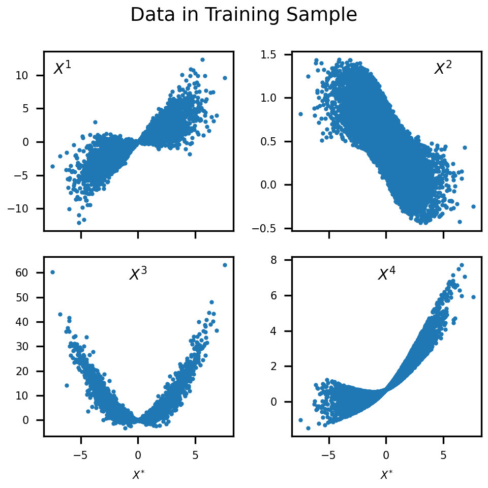
We sample 8000 points as training points from the above distributions for , , , and . Then we sample another 1000 points for validation points and 1000 points for test points. We draw 500 points from the training points with replacement 8000 times to build our training set and 1000 times from the validation/test points to build our validation/test set. Figure 1 shows the relationship between , , , and .

In the second experiment, we let the error terms correlate with while keeping the rest setup the same as the baseline. Figure 2 shows the relationship between , , , and in this one. Specifically, we use:
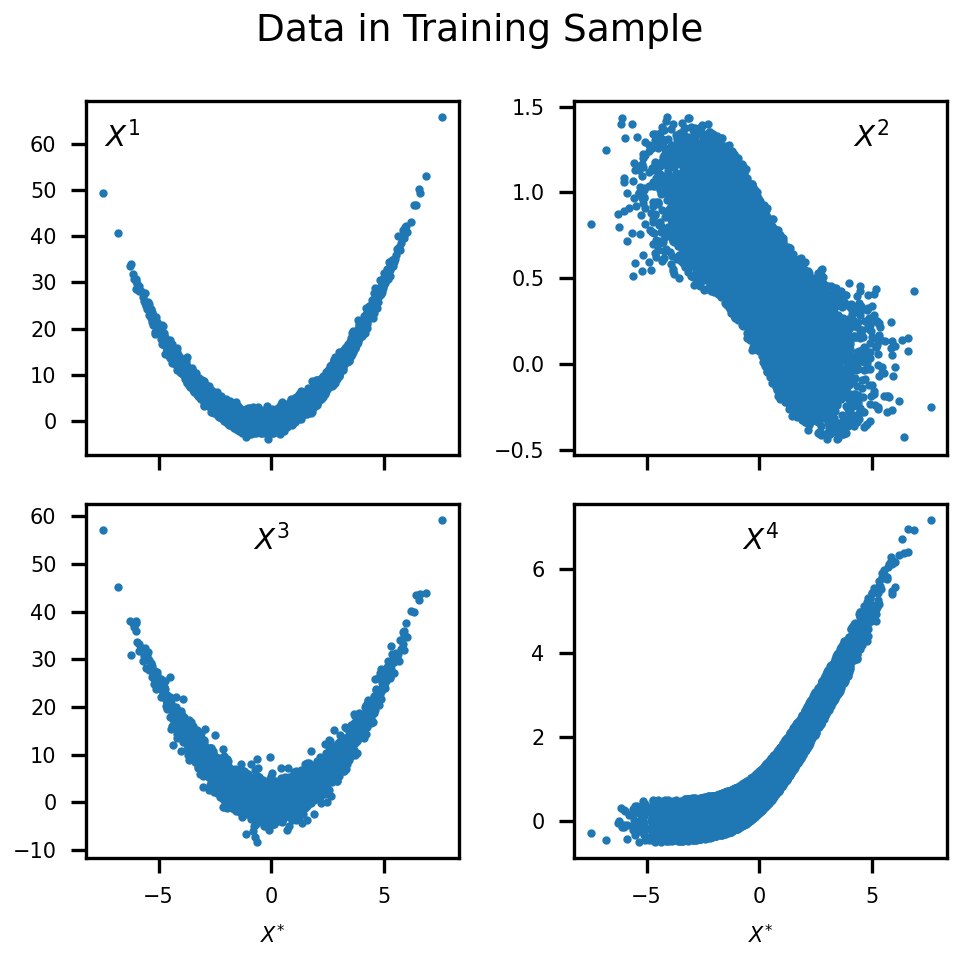
In the third experiment, we double the variance of the error terms while keeping the rest setup the same as the baseline. Figure 3 shows the relationship between , , , and in the third experiment.
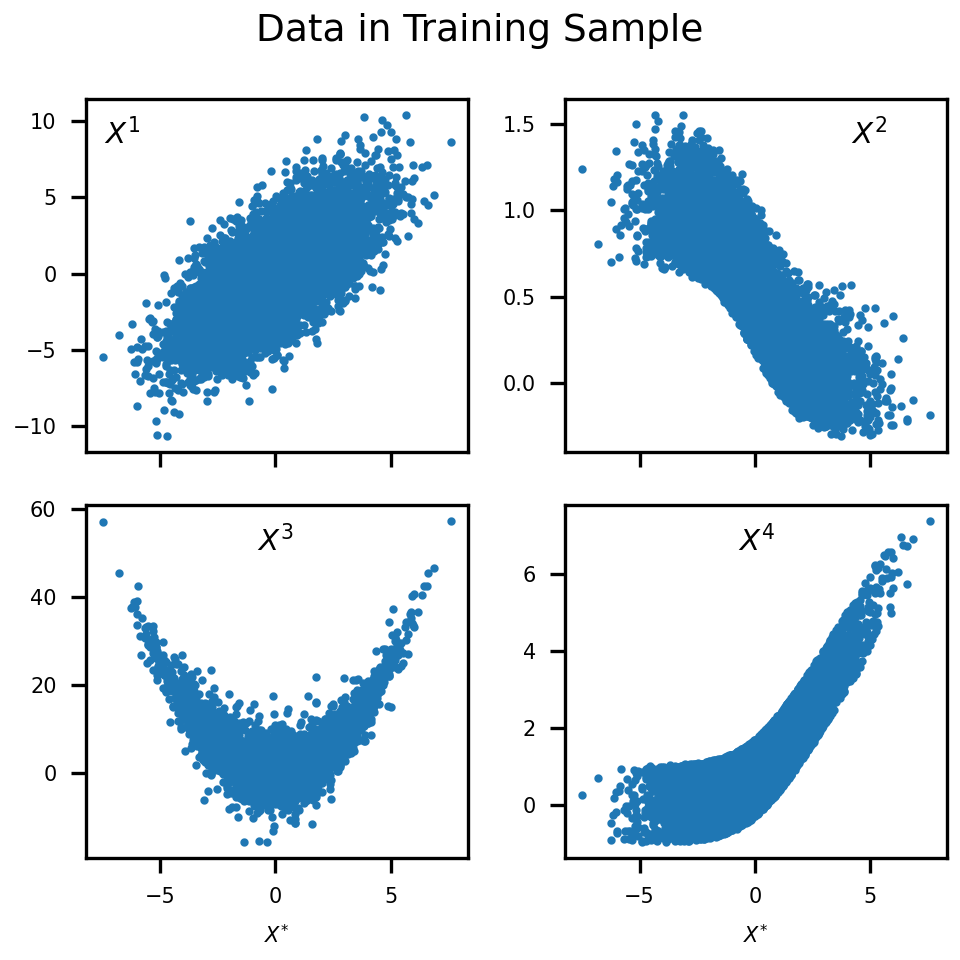
Table 1 demonstrates the min, median and max correlations of and in the test sample for the three experiments after running each one 25 times. Figure 4 shows their best runs respectively. It is clear that GEEN is robust with initialization with very tight distributions of the correlations of and and improves significantly if we simply use to directly measure .
| Simulation Name | corr(, ) | corr(, ) | ||
| min | median | max | ||
| Baseline | 0.97 | 0.98 | 0.98 | 0.89 |
| Linear Error | 0.94 | 0.96 | 0.97 | 0.89 |
| Double Error | 0.88 | 0.89 | 0.91 | 0.70 |

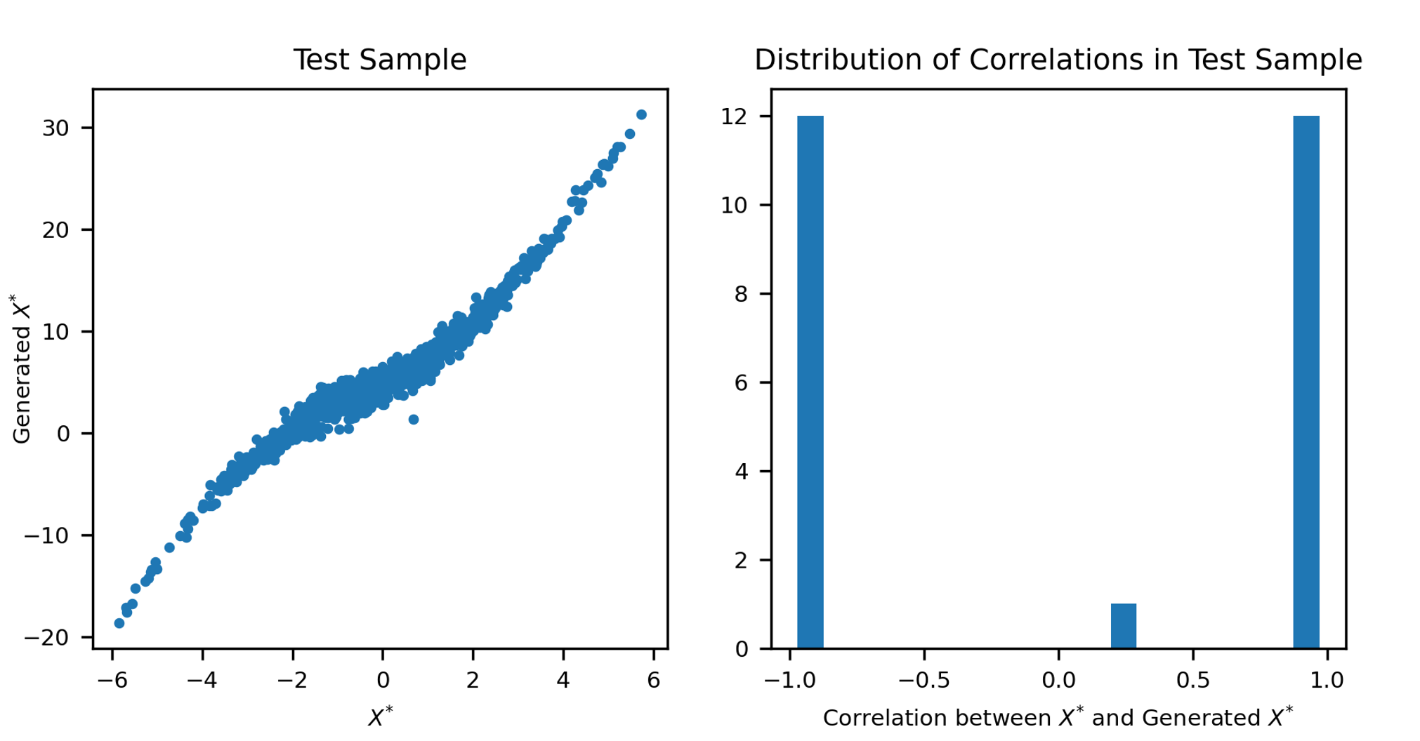
In the forth experiment, we loose the normalization condition while keeping the rest setup the same as the baseline. Figure 5 shows the relationship between , , , and in this experiment.
With this setup, generated is not anchored, and as shown in the left hand side of Figure 6 its values deviate significantly from . However, the KL loss helps keep the similarity of the two distributions of generated and . As shown in the right hand side of Figure 6, with 25 runs of this experiment most of the absolute values of the correlation between and are around 0.9. This suggests that even without normalization our framework can still help provide an estimation of the direction.
5 Summary
This paper proposes a Generative Element Extraction Networks (GEEN) to reveal unobserved variables in a random sample, which contains multiple measurements of a latent variable of interest. We present the sufficient conditions, under which the joint distribution of a latent variable and its measurements can be uniquely determined. We then argue that the true values of the latent variable in the sample are locally unique in a class of deviations, which allows us to estimate the true values. To the best of our knowledge, this paper is the first to provide such identification in observation. This approach is based on the key assumption that the measurements are independent conditional on the latent variable. We then propose an algorithm to minimize the probability densities with and without the conditional independence. We use the Kullback–Leibler distance between the two probability densities as the loss function to train the deep neutral network, which maps from the observed measurements to the true values of the latent variable in the sample. The simulation results imply that this proposed estimator works quite well and the estimated values are highly correlated with the true values with a correlation coefficient usually higher than 90%. We then apply this estimator to a panel data model to reveal the fixed effects (see our online appendix), which we believe is highly applicable to studies using longitudinal data. We expect this algorithm will change how researchers deal with latent variables in empirical research.
References
- Aigner et al. (1984) Aigner, D. J.; Hsiao, C.; Kapteyn, A.; and Wansbeek, T. 1984. Latent variable models in econometrics. Handbook of econometrics, 2: 1321–1393.
- Belghazi et al. (2018) Belghazi, M. I.; Baratin, A.; Rajeshwar, S.; Ozair, S.; Bengio, Y.; Courville, A.; and Hjelm, D. 2018. Mutual information neural estimation. In International conference on machine learning, 531–540. PMLR.
- Bishop (1998) Bishop, C. M. 1998. Latent variable models. In Learning in graphical models, 371–403. Springer.
- Darbellay and Vajda (1999) Darbellay, G. A.; and Vajda, I. 1999. Estimation of the information by an adaptive partitioning of the observation space. IEEE Transactions on Information Theory, 45(4): 1315–1321.
- Goodfellow et al. (2014) Goodfellow, I.; Pouget-Abadie, J.; Mirza, M.; Xu, B.; Warde-Farley, D.; Ozair, S.; Courville, A.; and Bengio, Y. 2014. Generative adversarial nets. Advances in neural information processing systems, 27.
- Holston, Laubach, and Williams (2017) Holston, K.; Laubach, T.; and Williams, J. C. 2017. Measuring the natural rate of interest: International trends and determinants. Journal of International Economics, 108: S59–S75.
- Hu (2017) Hu, Y. 2017. The econometrics of unobservables: Applications of measurement error models in empirical industrial organization and labor economics. Journal of econometrics, 200(2): 154–168.
- Hu and Schennach (2008) Hu, Y.; and Schennach, S. M. 2008. Instrumental variable treatment of nonclassical measurement error models. Econometrica, 76(1): 195–216.
- King and Morley (2007) King, T. B.; and Morley, J. 2007. In search of the natural rate of unemployment. Journal of Monetary Economics, 54(2): 550–564.
- Kingma and Welling (2013) Kingma, D. P.; and Welling, M. 2013. Auto-encoding variational bayes. arXiv preprint arXiv:1312.6114.
- Kullback and Leibler (1951) Kullback, S.; and Leibler, R. A. 1951. On information and sufficiency. The annals of mathematical statistics, 22(1): 79–86.
- Kuttner (1994) Kuttner, K. N. 1994. Estimating potential output as a latent variable. Journal of business & economic statistics, 12(3): 361–368.
- Laubach and Williams (2003) Laubach, T.; and Williams, J. C. 2003. Measuring the natural rate of interest. Review of Economics and Statistics, 85(4): 1063–1070.
- Lee and Park (2006) Lee, Y. K.; and Park, B. U. 2006. Estimation of Kullback–Leibler divergence by local likelihood. Annals of the Institute of Statistical Mathematics, 58(2): 327–340.
- Li, Jiang, and Marlin (2019) Li, S. C.-X.; Jiang, B.; and Marlin, B. 2019. Misgan: Learning from incomplete data with generative adversarial networks. arXiv preprint arXiv:1902.09599.
- Mattei and Frellsen (2019) Mattei, P.-A.; and Frellsen, J. 2019. MIWAE: Deep generative modelling and imputation of incomplete data sets. In International conference on machine learning, 4413–4423. PMLR.
- Moreno, Ho, and Vasconcelos (2003) Moreno, P.; Ho, P.; and Vasconcelos, N. 2003. A Kullback-Leibler divergence based kernel for SVM classification in multimedia applications. Advances in neural information processing systems, 16.
- Muzellec et al. (2020) Muzellec, B.; Josse, J.; Boyer, C.; and Cuturi, M. 2020. Missing data imputation using optimal transport. In International Conference on Machine Learning, 7130–7140. PMLR.
- Nazabal et al. (2020) Nazabal, A.; Olmos, P. M.; Ghahramani, Z.; and Valera, I. 2020. Handling incomplete heterogeneous data using vaes. Pattern Recognition, 107: 107501.
- Nguyen, Wainwright, and Jordan (2010) Nguyen, X.; Wainwright, M. J.; and Jordan, M. I. 2010. Estimating divergence functionals and the likelihood ratio by convex risk minimization. IEEE Transactions on Information Theory, 56(11): 5847–5861.
- Nowozin, Cseke, and Tomioka (2016) Nowozin, S.; Cseke, B.; and Tomioka, R. 2016. f-gan: Training generative neural samplers using variational divergence minimization. Advances in neural information processing systems, 29.
- Pérez-Cruz (2008) Pérez-Cruz, F. 2008. Kullback-Leibler divergence estimation of continuous distributions. In 2008 IEEE international symposium on information theory, 1666–1670. IEEE.
- Schennach (2020) Schennach, S. M. 2020. Mismeasured and unobserved variables. In Handbook of Econometrics, volume 7, 487–565. Elsevier.
- Wang, Kulkarni, and Verdú (2005) Wang, Q.; Kulkarni, S. R.; and Verdú, S. 2005. Divergence estimation of continuous distributions based on data-dependent partitions. IEEE Transactions on Information Theory, 51(9): 3064–3074.
- Wang, Kulkarni, and Verdú (2006) Wang, Q.; Kulkarni, S. R.; and Verdú, S. 2006. A nearest-neighbor approach to estimating divergence between continuous random vectors. In 2006 IEEE International Symposium on Information Theory, 242–246. IEEE.
- Yoon, Jordon, and Schaar (2018) Yoon, J.; Jordon, J.; and Schaar, M. 2018. Gain: Missing data imputation using generative adversarial nets. In International conference on machine learning, 5689–5698. PMLR.
- Yoon and Sull (2020) Yoon, S.; and Sull, S. 2020. GAMIN: Generative adversarial multiple imputation network for highly missing data. In Proceedings of the IEEE/CVF conference on computer vision and pattern recognition, 8456–8464.