Split-Spectrum Based Distributed State Estimation for Linear Systems^footnoteinfo

Lili Wang Email: lili.wang.zj@gmail.com Ji Liu Email: ji.liu@stonybrook.edu Brian D. O. Anderson Email: brian.anderson@anu.edu.au A. Stephen Morse Email: as.morse@yale.edu

Abstract

This paper studies a distributed state estimation problem for both continuous- and discrete-time linear systems. A simply structured distributed estimator {comprising interconnected local estimators} is first described for estimating the state of a continuous and multi-channel linear system whose sensed outputs are distributed across a fixed multi-agent network. The estimator is then extended to non-stationary networks whose graphs switch according to a switching signal. The estimator is guaranteed to solve the problem, provided a network-widely shared high gain condition achieving a form of spectrum separation is satisfied. As an alternative to sharing a common gain across the network, a fully distributed version of the estimator is also studied in which each agent adaptively adjusts a local gain, though the practicality of this approach is subject to a robustness issue common to adaptive control. A discrete-time version of the distributed state estimation problem is also studied, and a corresponding estimator based again on spectrum separation, but not high gain, is proposed for time-varying networks. For each scenario, it is explained how to construct the estimator so that the state estimation errors in the local estimators all converge to zero exponentially fast at a fixed but arbitrarily chosen rate, provided the network’s graph is strongly connected for all time. The proposed estimators are inherently resilient to abrupt changes in the number of agents and communication links in the inter-agent communication graph upon which the algorithms depend, provided the network is redundantly strongly connected and redundantly jointly observable.

keywords

Distributed Estimation, Multi-Agent Systems, Cooperative Control, Linear Systems

^†^†thanks: [^†^†address: Samueli School of Engineering, University of California, Irvine^†^†address: Department of Electrical and Computer Engineering, Stony Brook University^†^†address: Department of Electrical Engineering, Yale University^†^†address: School of Engineering, Australian National University

footnoteinfo]This paper was not presented at any IFAC meeting. Portions of this paper were presented at 2019 American Control Conference [1] and IEEE Conference on Decision and Control [2]. Corresponding author: Lili Wang.

, , ,

1 Introduction

With the growing interest in sensor networks and multi-agent systems, the problem of estimating the state of a dynamical system whose measured outputs are distributed across a network has been under study in one form or another for a number of years [3, 4, 5, 6, 7, 8, 9, 10, 11, 12, 13, 14, 15, 1].

Depending on the nature of the system to be estimated, the distributed estimation problem has continuous- and discrete-time versions. In its simplest form, the continuous-time version of the distributed state estimation problem starts with a network of $m>1$ agents labeled $1,2,\ldots,m$ which are able to receive information from their neighbors. Neighbor relations are characterized by a directed graph $\mathbb{N}$ , which may or may not depend on time, whose vertices correspond to agents and whose arcs depict neighbor relations. Each agent $i$ senses a signal $y_{i}\in{\rm I\!R}^{s_{i}},\;i\in\mathbf{m}\stackrel{{\scriptstyle\Delta}}{{=}}\{1,2,\ldots,m\}$ generated by a continuous-time system of the form $\dot{x}=Ax,\;y_{i}(t)=C_{i}x,\;i\in\mathbf{m}$ and $x\in{\rm I\!R}^{n}$ . It is typically assumed that $\mathbb{N}$ is strongly connected and that the system is jointly observable. It is invariably assumed that each agent receives certain real-time signals from its neighbors although what is received can vary from one problem formulation to the next. In all formulations, the goal is to devise local estimators, one for each agent, whose outputs are all asymptotically correct estimates of $x$ . The local estimator dynamics for agent $i$ are typically assumed to depend only on the pair $(C_{i},A)$ and certain properties of $\mathbb{N}$ . The problem is basically the same in discrete time, except that rather than the continuous-time model just described, the discrete-time model $x(\tau+1)=Ax(\tau),\;y_{i}(\tau)=C_{i}x(\tau),\;i\in\mathbf{m},\;x\in{\rm I\!R}^{n}$ is considered instead. More precise problem formulations will be given later.

1.1 Background

The study of distributed state estimation for linear systems can be dated back to the so-called distributed Kalman filter problem [16], which involves system and measurement noise in the problem formulation and has been widely studied for years [17, 3]. Most available Kalman filter based approaches [3, 6, 16, 17, 4] require the agents to both share “signal information”, which can be measurements or local state estimates, and fuse certain “structural information”, which forms the covariance or information matrix of the nominal centralized Kalman filter for each agent. For the problem just described, the existing literature based on only “signal information” sharing can be classified into two categories, namely continuous- and discrete-time estimators/observers, except for our earlier work of [15, 18] in which a hybrid observer was proposed for a continuous-time linear system.

Continuous-time distributed estimators have recently appeared in [1, 12, 13, 10, 14, 19]. By recasting and then solving the distributed estimation problem as a classical decentralized control problem, the resulting estimator becomes capable of estimating the state at a pre-assigned exponentially fast rate, assuming $\mathbb{N}$ is a constant strongly connected graph [10]. The work of [12] seeks to propose a distributed estimator for a continuous-time system at the expense of certain design flexibility. This is done, in essence, by exploiting the $A$ -invariance of the unobservable spaces of the pairs $(C_{i},A)$ ; this in turn enables one to “split” the local estimators into two parts, one based on conventional spectrum assignment techniques applied to the observable part of the state at each local estimator and the other based on consensus among the unobserved parts of the state at each local estimator. The two parts are interacting but the use of a high gain serves to simplify the stability issue because of a split in the spectrum arising from the design of the estimator. The idea has been further developed in [13, 14, 20]. Specifically, these latter references start to move beyond a restriction in [12] permitting only constant, undirected, connected neighbor graphs to be addressed. The work of [13, 14] extends the result of [12] to the case when the neighbor graph is constant, directed, strongly connected, while requiring that one chooses gains to ensure that certain LMIs hold which are difficult to grasp intuitively. In [21], motivated by a distributed least squares problem, a modified algorithm is proposed to deal with measurement noise constant, undirected, connected neighbor graphs. A distributed adaptive algorithm has recently been proposed in [20] which allows agents to join or leave the network over time, provided the resulting agent network always remains jointly connected and joint detectable. An evident disadvantage of all these existing continuous-time distributed estimators is that they require a somewhat complicated gain computation procedure, and partially because of this, do not, at least not directly, admit discrete-time counterparts.

Discrete-time distributed estimators have been recently studied in [22, 23, 24, 25, 9, 11, 26, 27, 28, 29]. Notable among them is the paper [9]. Published prior to the appearance of the early continuous time paper [10] applying to the same class of distributed systems, [9] solves the discrete-time distributed estimation problem for jointly observable, linear systems with constant, directed, strongly connected neighbor graphs. It builds on the idea of recasting the estimation problem as a classical decentralized control problem. Although the observer is limited to discrete-time systems, it has been proved possible to make use of the ideas in [9] to obtain, as noted earlier, a distributed observer for continuous-time systems [10], but still for constant neighbor graphs. There are however other discrete-time distributed observers/estimators which do not admit continuous-time extensions, illustrating that passage between discrete-time and continuous-time thinking may be harder than intuition initially suggests for distributed estimation problems. By expanding on earlier work in [11], the papers [26, 30] provide a procedure for constructing a centralized designed distributed observer for time-varying neighbor graphs. It requires the sharing of an index that records the age of the information across the network, and the agents are designed to act in a sequential manner to do state estimation. The resulting algorithm, which is tailored exclusively to discrete-time systems, requires a network-wide initialization step that serves to sort the agents in a specific order. Thereby it can deal with state estimation under assumptions that are weaker than strong connectivity.

Table 1. Comparison of Different Approaches to Design Distributed Estimators Nature of Approach Reference Continuous-time Systems Discrete-time Systems Exponential Convergence Time-varying Graphs Kalman Filter Based Approach [3, 6, 16, 17] ✗ ✓ ✗ ✗ [4] ✓ ✗ ✗ ✗ Observability Decomposition Based Approach [11] ✗ ✓ ✓ ✗ [26, 30] ✗ ✓ ✓ ✓ Decentralized Control Based Approach [9, 24, 25] ✗ ✓ ✓ ✗ [10, 19] ✓ ✗ ✓ ✗ Split-Spectrum Based Approach [1, 12, 13, 14] ✓ ✗ ✓ ✗ [2] ✗ ✓ ✓ ✗ This work ✓ ✓ ✓ ✓

Different approaches to the distributed state estimation problem are summarized in Table $1$ . It turns out that the current paper is the first paper that can deal with both continuous-time and discrete-time systems while ensuring exponential convergence under time-varying neighbor graphs.

The contribution of this paper rests on the following three distinguishing features, differentiating it and highlighting it as a development of earlier work:

•

The paper describes a simply structured, unified approach to the distributed state estimation problem and to design and analyze the corresponding distributed estimators for both continuous- and discrete-time linear systems with possibly time-varying graphs. It is termed the “split-spectrum” approach because it “splits” the system spectrum into disjoint subsets corresponding to observable and unobservable subspaces. In continuous time, this is achieved by a high gain mechanism, but in discrete-time by a different mechanism, viz. the adoption of two integrally related sampling rates. Though the mechanisms are instrumentally different, their purpose is fundamentally the same. It is termed ‘unified’ because the approach is shown to work for both continuous- and discrete-time linear systems over both constant and time-varying neighbor graphs.
•

A fully distributed version of the estimator is separately studied where each agent can adaptively adjust a local gain, with simpler gain computation procedure and analysis compared with [20].
•

Exponential convergence of the error dynamics is ensured with an arbitrarily assigned convergence rate. A great advantage of our methodology is that the designs and algorithms developed under a noiseless assumption are then necessarily tolerant of some level of noise, simply because we take care to ensure an exponential convergence.

It is assumed in this paper that the neighbor graph of the network is always strongly connected. From the perspective of the real world, requiring the underlying network to be strongly connected “at every time step” is an assumption that will occur in a great many (though obviously not all) cases, and as such, is deserving of a separate study in its own right. The extension to more general time-varying graphs is one future direction. It may not be conceptually difficult, however intricate the details may be.

The paper first describes the split-spectrum based distributed estimator for the case when the system dynamics are continuous with a stationary network in §2.1, and with associated background analysis is given in §2.2. The estimator is then extended to deal with non-stationary networks whose neighbor graphs switch according to a switching signal with a fixed dwell time or a variable dwell time with prescribed average, the ideas being detailed in §2.3. In the case when the interconnection among the agents can always be modelled usingdoubly stochastic matrices {e.g., undirected graphs with the Metropolis weights [5]}, it is shown in §2.3 that the estimator functions correctly even if the neighbor graph switches arbitrarily, provided the graph is always strongly connected. The estimators mentioned above all rely on the existence of a sufficiently large, network-widely shared gain. A fully distributed version of the estimator is then studied in §2.4 where each agent can adaptively adjust a local gain. The adaptive estimator is subject to a robustness issue common to adaptive control. The proposed estimators, except for the adaptive one, are inherently resilient to abrupt changes in the number of agents and communication links in the inter-agent communication graph upon which the algorithms depend, an issue which is discussed in §2.5. Then the split-spectrum based estimator design is extended to the case when the system dynamics is discrete in §3 for both constant and time-varying neighbor graphs. Simulation validation is provided in §4.

The material in this paper was partially presented in [1, 2], but this paper presents a more comprehensive treatment of the work. Specifically, the paper crafts continuous-time distributed estimators for two types of non-stationary networks in §2.3 and a fully distributed adaptive estimator in §2.4, which were not included in [1, 2].

2 Continuous-Time Distributed Estimator

We are interested in a network of $m>0$ {possibly mobile} autonomous agents labeled $1,2,\ldots,m$ which are able to receive information from their “neighbors”, where by a neighbor of agent $i$ is meant any other agent within agent $i$ ’s reception range. We write $\mathcal{N}_{i}(t)$ for the labels of agent $i$ ’s neighbors at time $t\in[0,\infty)$ and always take agent $i$ to be a neighbor of itself. Neighbor relations at time $t$ are characterized by a directed graph $\mathbb{N}(t)$ with $m$ vertices and a set of arcs defined so that there is an arc in $\mathbb{N}(t)$ from vertex $j$ to vertex $i$ whenever agent $j$ is a neighbor of agent $i$ at time $t$ . Since each agent $i$ is always a neighbor of itself, $\mathbb{N}(t)$ has a self-arc at each of its vertices. Each agent $i$ can sense a continuous-time signal $y_{i}\in{\rm I\!R}^{s_{i}},\;i\in\mathbf{m}\stackrel{{\scriptstyle\Delta}}{{=}}\{1,2,\ldots,m\}$ , where

	$\displaystyle y_{i}$	$\displaystyle=$	$\displaystyle C_{i}x,\;\;\;i\in\mathbf{m}$		(1)
	$\displaystyle\dot{x}$	$\displaystyle=$	$\displaystyle Ax$		(2)

and $x\in{\rm I\!R}^{n}$ . We assume throughout that $C_{i}\neq 0,\;i\in\mathbf{m}$ , and that the system defined by (1) and (2) is jointly observable; i.e., with $C=\begin{bmatrix}C_{1}^{\prime}&C_{2}^{\prime}&\cdots&C_{m}^{\prime}\end{bmatrix}^{\prime}$ , the matrix pair $(C,A)$ is observable. Joint observability is equivalent to the requirement that $\bigcap_{i\in\mathbf{m}}\mathcal{V}_{i}=0$ , where $\mathcal{V}_{i}$ is the unobservable space of $(C_{i},A)$ ; i.e. $\mathcal{V}_{i}=\ker\begin{bmatrix}C_{i}^{\prime}&(C_{i}A)^{\prime}&\cdots&(C_{i}A^{n-1})^{\prime}\end{bmatrix}^{\prime}$ . As is well known, $\mathcal{V}_{i}$ is the largest $A$ -invariant subspace contained in the kernel of $C_{i}$ . Generalizing the results that follow to the case when $(C,A)$ is only detectable is quite straightforward and can be accomplished using well-known ideas. However, the commonly made assumption that each pair $(C_{i},A),\;i\in\mathbf{m}$ , is observable, or even just detectable, is very restrictive, grossly simplifies the problem and is unnecessary. The assumption $C_{i}\neq 0$ is not necessary provided the more relaxed problem is properly formulated. The assumption is made for the sake of simplicity. The problem of interest is to construct a suitably defined family of linear estimators in such a way so that no matter what the estimators’ initial states are, each agent obtains an asymptotically correct estimate $x_{i}$ of $x$ in the sense that the estimation error $x_{i}(t)-x(t)$ converges to zero as fast as $\text{exp}(-\lambda t)$ does, where $\lambda$ is an arbitrarily chosen but fixed positive number.

This section proposes the estimator first, and then analyses the estimator beginning with the condition that the neighbor graph $\mathbb{N}(t)$ is constant. A time-varying neighbor graph $\mathbb{N}(t)$ is then considered in which changes occur according to a switching signal. Later, a fully distributed algorithm based on use of multiplicative adaptive gain control is developed.

2.1 The Estimator

The estimator to be considered consists of $m$ local or private estimators of the form for each $i\in\mathbf{m}$ ,

\dot{x}_{i}=(A+K_{i}C_{i})x_{i}-K_{i}y_{i}-gP_{i}\bigg(\!\!x_{i}-\frac{1}{m_{i}(t)}\!\!\!\sum_{j\in\mathcal{N}_{i}(t)}\!\!\!x_{j}\!\!\bigg)

(3)

where $m_{i}(t)$ is the number of labels in $\mathcal{N}_{i}(t)$ , $g$ is a suitably defined positive gain common to all local estimators, each $K_{i}$ is a suitably defined matrix, and for each $i\in\mathbf{m}$ , $P_{i}$ is the orthogonal projection on the unobservable space of $(C_{i},A)$ . The term $(A+K_{i}C_{i})x_{i}-K_{i}y_{i}$ is designed to enable each agent $i$ to be able to recover the observable part of the state by itself, and the term $-gP_{i}(x_{i}-\frac{1}{m_{i}(t)}\sum_{j\in\mathcal{N}_{i}(t)}x_{j})$ is for the purpose of utilizing information from its neighbors to recover the unobservable part of the state. It will be shown that with this design, the spectrum of the system matrix can be split into two subsets. Details on how to design the parameters $K_{i}$ and $g$ will be provided in the following.

2.1.1 The Error Dynamics

This subsection provides the error dynamics of the proposed estimator. It will be shown that the spectrum of the error system matrix can be split into two subsets based on the observability of each agent with $K_{i}$ defined properly.

First note from (3), that the state estimation error $e_{i}=x_{i}-x$ satisfies

\dot{e}_{i}=(A+K_{i}C_{i})e_{i}-gP_{i}\left(e_{i}-\frac{1}{m_{i}(t)}\sum_{j\in\mathcal{N}_{i}(t)}e_{j}\right)

(4)

Consequently the overall error vector $e=\begin{bmatrix}e_{1}^{\prime}\ \ldots\ e_{m}^{\prime}\end{bmatrix}^{\prime}$ satisfies

\dot{e}=(\bar{A}-gP(I_{mn}-\bar{S}(t)))e

(5)

where $\bar{A}=$ block diag $\{A+K_{1}C_{1},A+K_{2}C_{2},\ldots,A+K_{m}C_{m}\}$ , $P=$ block diag $\{P_{1},P_{2},\ldots,P_{m}\}$ , $\bar{S}(t)=S(t)\otimes I_{n}$ with $S(t)=D_{\mathbb{N}(t)}^{-1}\mathcal{A}^{\prime}_{\mathbb{N}(t)}$ . Here $I_{k}$ is the $k\times k$ identity matrix, and $\mathcal{A}_{\mathbb{N}(t)}$ is the adjacency matrix of $\mathbb{N}(t)$ and $D_{\mathbb{N}(t)}$ is the diagonal matrix whose $i$ th diagonal entry is the in-degree of $\mathbb{N}(t)$ ’s $i$ th vertex. Note that $\mathbb{N}(t)$ is the graph¹¹ 1 The graph of an $n\times n$ matrix $M$ is that directed graph on $n$ vertices possessing a directed arc from vertex $i$ to vertex $j$ if $m_{ij}\neq 0$ {p. 357, [31]}. of $S^{\prime}(t)$ and that the diagonal entries of $S^{\prime}(t)$ are all positive because each agent is a neighbor of itself. The matrix $S(t)$ is evidently a stochastic matrix.

Proposition 1

The spectrum of the error system matrix $\bar{A}-gP(I_{mn}-\bar{S})$ splits into two subsets. One subset contains the union of certain subsets of the eigenvalues associated with the $i$ -th local estimator, $i\in\mathbf{m}$ , these being able to be arbitrarily positioned by choice of the $K_{i}$ and independent of $g$ . The second subset is independent of the choice of the $K_{i}$ , and depends, though not to the extent of being able to be arbitrarily positioned, on $g$ .

We remark that in the proof below, we will explain how to choose the $K_{i}$ to ensure that the associated set of eigenvalues has degree of stability $\lambda$ (ensuring an estimation error decay at least as fast as $\exp(-\lambda t)$ ), while subsequently we will explain how to choose $g$ to ensure stability of the remaining part of the spectrum with the same minimum exponential decay rate.

Proof of Proposition 1: The definitions of $K_{i}$ and $g$ begin with the specification of a desired convergence rate bound $\lambda>0$ . To begin with, each matrix $K_{i}$ is defined as follows. For each fixed $i\in\mathbf{m}$ , write $Q_{i}$ for any full rank matrix whose kernel is the unobservable space of $(C_{i},A)$ and let $\bar{C}_{i}$ and $\bar{A}_{i}$ be the unique solutions to $\bar{C}_{i}Q_{i}=C_{i}$ and $Q_{i}A=\bar{A}_{i}Q_{i}$ respectively. Then the matrix pair $(\bar{C}_{i},\bar{A}_{i})$ is observable. A matrix $\bar{K}_{i}$ can be chosen to ensure that the convergence of $\text{exp}\{(\bar{A}_{i}+\bar{K}_{i}\bar{C}_{i})t\}$ to zero is as fast as the convergence of $\text{exp}(-\lambda t)$ to zero is. There are several well-documented ways to do this {e.g, spectrum assignment algorithms or Riccati equation solvers}, since each pair $(\bar{C}_{i},\bar{A}_{i})$ is observable. Having chosen such $\bar{K}_{i}$ , $K_{i}$ is then chosen to be $K_{i}=Q_{i}^{-1}\bar{K}_{i}$ where $Q_{i}^{-1}$ is a right inverse for $Q_{i}$ . The definition implies that

Q_{i}(A+K_{i}C_{i})=(\bar{A}_{i}+\bar{K}_{i}\bar{C}_{i})Q_{i}

(6)

and that $(A+K_{i}C_{i})\mathcal{V}_{i}\subset\mathcal{V}_{i}$ . The latter, in turn, implies that there is a unique matrix $A_{i}$ which satisfies

(A+K_{i}C_{i})V_{i}=V_{i}A_{i}

(7)

where $V_{i}$ is a basis matrix²² 2 For simplicity, we assume that the columns of $V_{i}$ constitute an orthonormal basis for $\mathcal{V}_{i}$ in which case $P_{i}=V_{i}V_{i}^{\prime}$ . for $\mathcal{V}_{i}$ .

Next we show what defining the $K_{i}$ in this way accomplishes. Note that the subspace $\mathcal{V}=\mathcal{V}_{1}\oplus\mathcal{V}_{2}\oplus\cdots\oplus\mathcal{V}_{m}$ is $\bar{A}$ - invariant because $(A+K_{i}C_{i})\mathcal{V}_{i}\subset\mathcal{V}_{i},\;i\in\mathbf{m}$ . Next, let $Q=$ block diag $\{Q_{1},Q_{2},\ldots,Q_{m}\}$ and $V=$ block diag $\{V_{1},V_{2},\ldots,V_{m}\}$ where $V_{i}$ is a matrix whose columns form an orthonormal basis for $\mathcal{V}_{i}$ . Then $Q$ is a full rank matrix whose kernel is $\mathcal{V}$ and $V$ is a basis matrix for $\mathcal{V}$ whose columns form an orthonormal set. It follows that $P=VV^{\prime}$ , that $QP=0$ , and that

	$\displaystyle Q\bar{A}$	$\displaystyle=$	$\displaystyle\bar{A}_{V}Q$		(8)
	$\displaystyle\bar{A}V$	$\displaystyle=$	$\displaystyle V\tilde{A}$		(9)

where $\tilde{A}=\text{block diag}\;\{A_{1},A_{2},\ldots,A_{m}\}$ and

\bar{A}_{V}=\text{block diag}\;\{\bar{A}_{1}+\bar{K}_{1}\bar{C}_{1},\ldots,\bar{A}_{m}+\bar{K}_{m}\bar{C}_{m}\}.

(10)

Let $V^{-1}$ be any left inverse for $V$ and let $Q^{-1}$ be that right inverse for $Q$ for which $V^{-1}Q^{-1}=0$ . Then

\bar{A}-gP(I_{mn}-\bar{S}(t))=T\begin{bmatrix}\bar{A}_{V}&0\\ \hat{A}_{V}(t)&A_{V}(t)\end{bmatrix}T^{-1}

(11)

where $\hat{A}_{V}(t)=V^{-1}(\bar{A}-g(I_{mn}-\bar{S}(t)))Q^{-1}$ and $A_{V}(t)=\tilde{A}-gV^{\prime}(I_{mn}-\bar{S}(t))V.$ Here $T=\begin{bmatrix}Q^{-1}&V\end{bmatrix}$ . It is easy to check that $T^{-1}=\begin{bmatrix}Q^{\prime}&V\end{bmatrix}^{\prime}$ .

According to (11), the spectrum of $\bar{A}-gP(I_{mn}-\bar{S})$ is equivalent to the union of the spectrum of $\bar{A}_{V}$ and $A_{V}$ .

Recall that the $\bar{K}_{i}$ have been already been chosen so that each matrix exponential $\text{exp}\{(\bar{A}_{i}+\bar{K}_{i}\bar{C}_{i})t\}$ converges to zero as fast as $\text{exp}({-\lambda t})$ does. Because of this and the fact that $\hat{A}_{V}(t)$ is a bounded matrix, to ensure that for each fixed $\tau$ , the state transition matrix $\Phi(t,\tau)$ converges to zero as fast as $\text{exp}({-\lambda t})$ does, it is enough to choose $g$ so that the state transition matrix of $A_{V}(t)$ converges to zero at least as fast as $\text{exp}({-\lambda t})$ does. The requisite condition on $g$ is provided below for three different neighbor graph connectivity assumptions.

2.2 Constant Neighbor Graph

This subsection focuses on the case when the neighbor graph $\mathbb{N}(t)$ is a constant graph $\mathbb{N}$ . The following result can be obtained.

Theorem 1

For any given positive number $\lambda$ , if the neighbor graph $\mathbb{N}$ is fixed and strongly connected, and the system defined by (1) and (2) is jointly observable, there are matrices $K_{i}$ , $i\in\mathbf{m}$ such that for $g$ sufficiently large, each estimation error $x_{i}(t)-x(t)$ of the distributed estimator defined by (3), converges to zero as $t\rightarrow\infty$ as fast as $\text{exp}({-\lambda t})$ converges to zero.

The proof of the theorem involves making use of the following result, with all proofs being contained in Appendix A. In particular, the proof of Proposition 2 makes use of the properties of strong connectivity of the neighbor graph and joint observability of the system.

Proposition 2

$-V^{\prime}(I_{mn}-\bar{S})V$ is a continuous-time stability matrix.

2.3 Switching Neighbor Graph

In the sequel the problem is studied under the assumption that $\mathbb{N}(t)$ changes according to a switching signal with a fixed dwell time or a variable dwell time with fixed average. To characterize the assumed time dependence of $\mathbb{N}(t)$ , let $\mathcal{G}=\{\mathbb{G}_{1},\mathbb{G}_{2},\ldots,\mathbb{G}_{n_{g}}\}$ denote the set of all directed, strongly connected graphs on $m$ vertices which have self-arcs at all vertices; here $n_{g}$ is the number of graphs in $\mathcal{G}$ . In some situations, the switching signals always have consecutive discontinuities separated by a value which is no less than a fixed positive real number $\tau_{D}$ . It is called a dwell time [32]. In certain situations, the switching signals may occasionally have consecutive discontinuities separated by less than $\tau_{D}$ , but for which the average interval between consecutive discontinuities is no less than $\tau_{D}$ . This leads to the concept of an average dwell-time. With $\tau_{D}$ and $\delta$ fixed define $\mathcal{S}_{\text{avg}}$ for the set of all piecewise-constant switching signals $\sigma:[0,\infty)\rightarrow\{1,2,\ldots,|\mathcal{G}|\}$ satisfying $\delta_{\sigma}(t_{0},t)\leq\delta_{0}+\frac{t-t_{0}}{\tau_{D}}$ . Here $\delta_{\sigma}(t_{0},t)$ denotes the number of discontinuities of $\sigma$ in the open interval $(t_{0},t)$ . The constant $\tau_{D}$ is called the average dwell-time and $\delta_{0}$ the chatter bound [33]. By the set of all time-varying neighbor graphs with average dwell-time $\tau_{D}$ is meant the set $\{\mathbb{G}_{\sigma}:\sigma\in\mathcal{S}_{\text{avg}}\}$ . Note that switching according to a dwell time is a special case of switching according to an average dwell time. In the following, it is assumed that $\mathbb{N}\in\{\mathbb{G}_{\sigma}:\sigma\in\mathcal{S}_{\text{avg}}\}$ .

The problem to which this subsection is addressed is this. For fixed averaged dwell-time $\tau_{D}$ and the chatter bound $\delta_{0}$ , devise a procedure for crafting $m$ local estimators, one for each agent, so that for each neighbor graph $\mathbb{N}\in\{\mathbb{G}_{\sigma}:\sigma\in\mathcal{S}_{\text{avg}}\}$ , all $m$ state estimation errors converge to zero exponentially fast at a prescribed rate.

The estimator to be considered is still the same as the estimator described in (3), with the exception that $g$ is chosen differently. The following result can be derived.

Theorem 2

For any fixed positive numbers $\tau_{D}$ and $\lambda$ , there exists a positive number $g^{*}$ with the following property. For any value of $g\geq g^{*}$ , any neighbor graph $\mathbb{N}\in\{\mathbb{G}_{\sigma}:\sigma\in\mathcal{S}_{\text{avg}}\}$ , if the system defined by (1) and (2) is jointly observable, there are matrices $K_{i},\;i\in\mathbf{m}$ such that, each state estimation error $e_{i}=x_{i}-x,\;i\in\mathbf{m}$ of the distributed estimator defined by (3) converges to zero as $t\rightarrow\infty$ as fast as $\text{exp}({-\lambda t})$ does.

The proof of Theorem 2 depends on the following lemma.

Lemma 1

Let $M_{1},M_{2},\ldots,M_{|\mathcal{G}|}$ be a set of $n\times n$ exponentially stable real matrices associated with a set $\mathcal{G}=\{\mathbb{G}_{1},\mathbb{G}_{2},\dots,\mathbb{G}_{|\mathcal{G}|}\}$ of directed strongly connected graphs with self-arcs at all vertices. Let $\sigma$ denote the switching signal with average dwell time $\tau_{D}$ governing the selection of a graph from $\mathcal{G}$ . Then for any $n\times n$ real matrix $N$ and positive number $\lambda$ there is a positive number $g^{*}$ , depending on $\tau_{D}$ for which, for each $\sigma\in\mathcal{S}_{\text{avg}}$ and $g\geq g^{*}$ , all solutions to

\dot{x}=(N+gM_{\sigma})x

(12)

converge to zero as fast as $\text{exp}({-\lambda t})$ does.

The proofs of Lemma 1 and Theorem 2 can be found in Appendix A.

In the sequel the problem is studied for a certain type of switching neighbor graphs. It turns out that if the stochastic matrices of undirected neighbor graphs are chosen to be doubly stochastic, there exist estimators which can deal with arbitrary switching signals, and the notion of dwell times ceases to be relevant. The estimator to be considered is again the same as (3), with the exception that $g$ is chosen differently.

Theorem 3

For any fixed positive number $\lambda$ , there exists a positive number $g^{*}$ with the following property. For any value of $g\geq g^{*}$ , any time-varying neighbor graph $\mathbb{N}(t)$ , if the system defined by (1) and (2) is jointly observable, the neighbor graph $\mathbb{N}(t)$ is undirected and connected, and the stochastic matrix $S(t)$ of graph $\mathbb{N}(t)$ is doubly stochastic, there are matrices $K_{i},\;i\in\mathbf{m}$ such that each state estimation error $x_{i}(t)-x(t)$ of the distributed observer defined by (3), converges to zero as $t\rightarrow\infty$ as fast as $\text{exp}({-\lambda t})$ converges to zero.

The proof of Theorem 3 can be found in Appendix A.

Given that $\tilde{A}$ has eigenvalues which are a subset of those of $A$ , it is seen that the effect of large $g$ is to force the instantaneous value of the eigenvalues of $A_{V}(t)$ well to the left of those of $\tilde{A}$ , and indeed the same for the Lyapunov exponent. This is a spectral separation idea – consensus dynamics within the estimator are faster than those of the original system.

2.4 Distributed Estimator with Adaptive Gains

Obviously it may be disadvantageous to share a gain across the whole network, and here we aim to design a simple adaptive distributed estimator to get gains for each estimators in a distributed way. The estimator for each agent $i$ still has the form (3) while each agent $i$ has its own gain $g_{i}$ which is obtained by

\dot{g}_{i}=\Big|V_{i}^{\prime}\sum_{j\in\mathcal{N}_{i}}\frac{1}{m_{i}}(x_{j}-x_{i})\Big|_{2}^{2},\;\;\;i\in\mathbf{m}

(13)

where $|\cdot|_{2}$ denotes the two norm of a matrix and $g_{i}(0)$ is nonnegative but otherwise arbitrary. Key questions arising are whether the $g_{i}$ are bounded, and whether the matrices $K_{i}$ can be chosen in the same way as previously. We have in fact with $K_{i}$ chosen as in the proof of Proposition 1:

Theorem 4

For any neighbor graph $\mathbb{N}\in\{\mathbb{G}_{\sigma}:\sigma\in\mathcal{S}_{\text{avg}}\}$ , if the system defined by (1) and (2) is jointly observable, and the gain is defined by (13), there are matrices $K_{i},\;i\in\mathbf{m}$ such that all the $g_{i}$ are bounded, and each state estimation error $e_{i}=x_{i}-x$ of the distributed estimator defined by (3) asymptotically converges to zero as $t\rightarrow\infty$ .

The proof of Theorem 4 can be found in Appendix A.

As with any adaptive control algorithm, we must recognize that there are fundamental challenges that can arise in practice and have the potential to undermine the approach [34]: these include the need to work with models of plants that may be very accurate but are virtually never exact; the inability to know, given an unknown plant, whether a desired control objective is practical or impractical, and the possibility of transient instability, or extremely large signals occurring before convergence. Thus, for this paper, our preference is to stick with a given $g$ instead of using an adaptive algorithm.

2.5 Resilience

The concept of a passively resilient algorithm is proposed in [18]. By a passively resilient algorithm for a distributed process is meant an algorithm which, by exploiting built-in network and data redundancies, is able to continue to function correctly in the face of abrupt changes in the number of vertices and arcs in the inter-agent communication graph upon which the algorithm depends. All the proposed continuous-time distributed estimators, except for the adaptive one, are inherently resilient to these abrupt changes provided the network is redundantly strongly connected and redundantly jointly observable, with a careful gain picking before the algorithm starts. Details can be found in Section 5 of [18]. The same resilience property is also possessed by the discrete-time distributed estimators to be developed in the next section.

3 Discrete-Time Distributed Estimator

In this section, a discrete time version of the distributed estimator problem is studied. The estimator which solves this problem in discrete time is described. Of central concern is the achieving of the split spectrum property, which underpins a stability guarantee for the estimator. High gain is not the answer: in continuous time, this produced a split spectrum (with some very fast modes). The discrete-time analogy rests on having part of the spectrum in the estimator achieved by gains $K_{i}$ as in continuous-time and partly determined by the dynamics creating consensus among the components of local estimated states corresponding to unobserved components of the underlying system state, with the associated time scale significantly faster than the single time scale associated with the underlying system dynamics. The second time scale is made possible through the introduction of a faster sampling rate.

We are interested in the same time-varying network as used for the continuous-time linear system and which is characterized by the neighbor graph $\mathbb{N}(t)$ . Each agent $i$ can sense a discrete-time signal $y_{i}(\tau)\in{\rm I\!R}^{s_{i}}$ at event times $\tau T$ , $\tau=0,1,2,\ldots$ where $T$ is a positive constant; for $i\in\mathbf{m}$ and $\tau=0,1,2,\ldots$

y_{i}(\tau)=C_{i}x(\tau),\;\;\;\;\;x(\tau+1)=Ax(\tau)

(14)

and $x\in{\rm I\!R}^{n}$ . We assume throughout that $\mathbb{N}(t)$ is strongly connected, and the system defined by (14) is jointly observable.

Each agent $i$ is to estimate $x$ using a dynamical system whose output $x_{i}(\tau)\in{\rm I\!R}^{n}$ is to be an asymptotically correct estimate of $x(\tau)$ in the sense that the estimation error $x_{i}(\tau)-x(\tau)$ converges to zero as $\tau\rightarrow\infty$ as fast as $\lambda^{\tau}$ does, where $\lambda$ is an arbitrarily chosen but fixed positive number³³ 3 For the type of observer to be developed, finite-time convergence is not possible. less than $1$ . To accomplish this it is assumed that the information agent $i$ can receive from neighbor $j$ at event time $\tau T$ is $x_{j}(\tau)$ . It is further assumed that agent $i$ can also receive certain additional information from its neighbors at a finite number of times between each successive pair of event times; what this information is will be specified below.

3.1 The Estimator

In this section it will be assumed that each agent’s neighbors do not change between event times. In other words, for $i\in\mathbf{m}$ ,

\mathcal{N}_{i}(t)=\mathcal{N}_{i}(\tau T),\;\;\;\;t\in[\tau T,(\tau+1)T),\;\;\;\;\tau=0,1,2,\ldots

With this assumption, the estimator to be considered consists of $m$ private estimators, one for each agent. The estimator for agent $i$ is of the form

x_{i}(\tau+1)=(A+K_{i}C_{i})\bar{x}_{i}(\tau)-K_{i}y_{i}(\tau)

(15)

where $\bar{x}_{i}(\tau)$ is an “averaged state” computed recursively over $q$ steps during the real time interval $[\tau T,\;(\tau+1)T)$ using the update equations

$\displaystyle z_{i}(0,\tau)$	$\displaystyle=$	$\displaystyle x_{i}(\tau)$	(16)
$\displaystyle z_{i}(k,\tau)$	$\displaystyle=$	$\displaystyle(I-P_{i})z_{i}(k-1,\tau)+$	(17)
		$\displaystyle\frac{1}{m_{i}(\tau)}P_{i}\!\!\!\!\sum_{j\in\mathcal{N}_{i}(\tau T)}\!\!\!\!z_{j}(k-1,\tau),\;\;k\in\mathbf{q}$	(17)
$\displaystyle\bar{x}_{i}(t)$	$\displaystyle=$	$\displaystyle z_{i}(q,\tau)$	(18)

Here $m_{i}(\tau)$ is the number of labels in $\mathcal{N}_{i}(\tau T)$ , $q$ is a suitably defined positive integer, further detail being given below, $\mathbf{q}=\{1,2,\ldots,q\}$ , and $P_{i}$ is the orthogonal projection on the unobservable space of $(C_{i},A)$ . Each matrix $K_{i}$ is defined as explained in the next paragraph. Meanwhile, we note that the estimators incorporate two time scales. An agent’s local estimator obtains data from its neighbors at a rate $q$ times that at which it obtains measurement data from the underlying system.

As described in §2.1, for fixed $i\in\mathbf{m}$ , write $Q_{i}$ for any full rank matrix whose kernel is the unobservable space of $(C_{i},A)$ , and let $\bar{C}_{i}$ and $\bar{A}_{i}$ be the unique solutions to $\bar{C}_{i}Q_{i}=C_{i}$ and $Q_{i}A=\bar{A}_{i}Q_{i}$ respectively. Let $\lambda$ be a positive value bounded by $1$ . Then the matrix pair $(\bar{C}_{i},\bar{A}_{i})$ is observable. Thus by using a standard spectrum assignment algorithm, a matrix $\bar{K}_{i}$ can be chosen to ensure that the convergence of $(\bar{A}_{i}+\bar{K}_{i}\bar{C}_{i})^{\tau}$ to zero as $\tau\rightarrow\infty$ is as fast as the convergence to zero of $\lambda^{\tau}$ . Having chosen such $\bar{K}_{i}$ , $K_{i}$ is then defined to be $K_{i}=Q_{i}^{-1}\bar{K}_{i}$ where $Q_{i}^{-1}$ is a right inverse for $Q_{i}$ . To explain what needs to be considered in choosing $q$ , which is a rough analog of the gain $g$ of the continuous-time solution, it is necessary to describe the structure of the “error model” of the overall estimator. This will be done next.

3.1.1 The Error Dynamics

For $i\in\mathbf{m}$ , write $e_{i}(\tau)$ for the state estimation error $e_{i}(\tau)=x_{i}(\tau)-x(\tau)$ . In view of (15),

e_{i}(\tau+1)=(A+K_{i}C_{i})\bar{e}_{i}(\tau)

where $\bar{e}_{i}(\tau)=\bar{x}_{i}(\tau)-x(\tau)$ . Moreover if $\epsilon_{i}(k,\tau)\stackrel{{\scriptstyle\Delta}}{{=}}z_{i}(k,\tau)-x(\tau),\;k\in\{0,1,\ldots,q\}$ then for $k\in\mathbf{q}$ ,

$\displaystyle\epsilon_{i}(0,\tau)$	$\displaystyle=$	$\displaystyle e_{i}(\tau)$
$\displaystyle\epsilon_{i}(k,\tau)$	$\displaystyle=$	$\displaystyle(I-P_{i})\epsilon_{i}(k-1,\tau)\!+\!\frac{1}{m_{i}(\tau)}P_{i}\!\!\!\!\!\sum_{j\in\mathcal{N}_{i}(\tau T)}\!\!\!\!\!\epsilon_{j}(k-1,\tau\!)$
$\displaystyle\bar{e}_{i}(\tau)$	$\displaystyle=$	$\displaystyle\epsilon_{i}(q,\tau)$

because of (16) – (18). It is possible to combine these $m$ subsystems into a single system. Paralleling §2.1.1 let $e=$ col $\{e_{1},e_{2},\ldots,e_{m}\}$ , define $\bar{A}=$ block diag $\{A+K_{1}C_{1},A+K_{2}C_{2},\ldots,A+K_{m}C_{m}\}$ , $P=$ block diag $\{P_{1},P_{2},\ldots,P_{m}\}$ and write $S(\tau)$ for the stochastic matrix $S(\tau)=D_{\mathbb{N}(\tau T)}^{-1}\mathcal{A}^{\prime}_{\mathbb{N}(\tau T)}$ where $\mathcal{A}_{\mathbb{N}(\tau T)}$ is the adjacency matrix of $\mathbb{N}(\tau T)$ and $D_{\mathbb{N}(\tau T)}$ is the diagonal matrix whose $i$ th diagonal entry is the in-degree of $\mathbb{N}(\tau T)$ ’s $i$ th vertex. Let $\bar{e}(\tau)=$ col $\{\bar{e}_{1}(\tau),\bar{e}_{2}(\tau),\ldots,\bar{e}_{m}(\tau)\}$ and $\epsilon(k,\tau)=\text{col}\{\epsilon_{1}(k,\tau),\epsilon_{2}(k,\tau),\ldots,\epsilon_{m}(k,\tau)\}$ . Then

e(\tau+1)=\bar{A}\bar{e}(\tau)

and

$\displaystyle\epsilon(0,\tau)$	$\displaystyle=$	$\displaystyle e(\tau)$
$\displaystyle\epsilon(k,\tau)$	$\displaystyle=$	$\displaystyle(I_{mn}-P(I_{mn}-\bar{S}(\tau)))\epsilon(k-1,\tau),\;k\in\mathbf{q}$
$\displaystyle\bar{e}(\tau)$	$\displaystyle=$	$\displaystyle\epsilon(q,\tau)$

where $\bar{S}(\tau)=S(\tau)\otimes I_{n}$ . Clearly $\bar{e}(\tau)=(I_{mn}-P(I_{mn}-\bar{S}(\tau)))^{q}e(\tau)$ , so

e(\tau+1)=\bar{A}(I_{mn}-P(I_{mn}-\bar{S}(\tau)))^{q}e(\tau)

(19)

Our immediate aim is now to explain why for $q$ sufficiently large, the time-varying matrix $\bar{A}(I_{mn}-P(I_{mn}-\bar{S}(\tau)))^{q}$ appearing in (19) is a discrete-time stability matrix for which the product

\Phi(\tau)=\prod_{s=1}^{\tau}\bar{A}(I_{mn}-P(I_{mn}-\bar{S}(s)))^{q}

(20)

converges to zero as $\tau\rightarrow\infty$ as fast as $\lambda^{\tau}$ does.

To begin with, we explore the propoerty of matrix $\bar{A}(I_{mn}-P(I_{mn}-\bar{S}(\tau)))^{q}$ .

Proposition 3

The spectrum of the error system matrix $\bar{A}(I_{mn}-P(I_{mn}-\bar{S}(\tau)))^{q}$ splits into two subsets. One subset contains the union of certain subsets of the eigenvalues associated with the $i$ -th local estimator, $i\in\mathbf{m}$ , these being able to be arbitrarily positioned by choice of the $K_{i}$ and independent of $q$ . The second subset is independent of the choice of the $K_{i}$ and depends, though not to the extent of being able to be arbitrarily positioned, on $q$ .

Proof of Proposition 3: As described in §2.1, note that the subspace $\mathcal{V}=\mathcal{V}_{1}\oplus\mathcal{V}_{2}\oplus\cdots\oplus\mathcal{V}_{m}$ is $\bar{A}$ - invariant because $(A+K_{i}C_{i})\mathcal{V}_{i}\subset\mathcal{V}_{i},\;i\in\mathbf{m}$ . Next, let $Q=$ block diag $\{Q_{1},Q_{2},\ldots,Q_{m}\}$ and $V=$ block diag $\{V_{1},V_{2},\ldots,V_{m}\}$ It follows that $P=VV^{\prime}$ , (8) and (9). Also as before, $(A+K_{i}C_{i})V_{i}=V_{i}A_{i}$ . Moreover

	$\displaystyle Q(I_{mn}-P(I_{mn}-\bar{S}(\tau)))^{q}$	$\displaystyle=$	$\displaystyle Q$		(21)
	$\displaystyle(I_{mn}-P(I_{mn}-\bar{S}(\tau)))^{q}V$	$\displaystyle=$	$\displaystyle V(V^{\prime}\bar{S}(\tau)V)^{q}$		(22)

Note that (21) holds because $QP=0$ . To understand why (22) is true, note first that $(I_{mn}-P(I_{mn}-\bar{S}(\tau)))V=V(I_{\bar{n}}-V^{\prime}(I_{mn}-\bar{S}(\tau))V)$ because $P=VV^{\prime}$ ; here $\bar{n}=\dim(\mathcal{V})$ . But $I_{\bar{n}}-V^{\prime}(I_{mn}-\bar{S}(\tau))V=V^{\prime}\bar{S}(\tau)V$ because $V^{\prime}V=I_{\bar{n}}$ . Thus (22) holds for $q=1$ ; it follows by induction that (22) holds for any positive integer $q$ .

Using (8), (9),(21), and (22), one obtains the equations

	$\displaystyle Q\bar{A}(I_{mn}-P(I_{mn}-\bar{S}(\tau)))^{q}$	$\displaystyle=$	$\displaystyle\bar{A}_{V}Q$		(23)
	$\displaystyle\bar{A}(I_{mn}-P(I_{mn}-\bar{S}(\tau)))^{q}V$	$\displaystyle=$	$\displaystyle VA_{V}(\tau)$		(24)

where

A_{V}(\tau)=\tilde{A}(V^{\prime}\bar{S}(\tau)V)^{q}

(25)

with $\tilde{A}=\text{block diag }\{A_{1},A_{2},\ldots,A_{m}\}$ . These equations imply that⁴⁴ 4 The notation $\hat{A}_{V}$ and $A_{V}$ are different from the two defined in §2.

\bar{A}(I_{mn}-P(I_{mn}-\bar{S}(\tau)))^{q}=T\begin{bmatrix}\bar{A}_{V}&0\\ \hat{A}_{V}(\tau)&A_{V}(\tau)\end{bmatrix}T^{-1}

(26)

with $T=\begin{bmatrix}Q^{-1}&V\end{bmatrix}$ and $\widehat{A}_{V}(\tau)=V^{-1}\bar{A}(I_{mn}-P(I_{mn}-\bar{S}(\tau)))^{q}Q^{-1}$ .

According to (26), the spectrum of $\bar{A}(I_{mn}-P(I_{mn}-\bar{S}(\tau)))^{q}$ is equivalent to the union of the spectrum of $\bar{A}_{V}$ and $A_{V}(\tau)$ .

3.2 Time-varying Neighbor Graph

The following result can be obtained when the neighbor graph is time-varying but strongly connected.

Theorem 5

For any given $\lambda$ with $|\lambda|<1$ , if the neighbor graph $\mathbb{N}(\tau)$ is strongly connected, and the system defined by (14) is jointly observable, there are matrices $K_{i}$ , $i\in\mathbf{m}$ such that for sufficiently large $q$ , each estimation error $x_{i}(\tau)-x(\tau)$ of the distributed estimator defined by (15)-(18), converges to zero as $\tau\rightarrow\infty$ as fast as $\lambda^{\tau}$ converges to zero.

The proof of the theorem involves studying the transition matrix and making use of the following results, with all proofs being contained in Appendix B.

Lemma 2

Let $M$ be an $m\times m$ row stochastic matrix which has a strongly connected graph. There exists a diagonal matrix $\Pi_{M}$ whose diagonal entries are positive for which the matrix $L_{M}=\Pi_{M}-M^{\prime}\Pi_{M}M$ is positive semi-definite; moreover $L_{M}\mathbf{1}=0$ where $\mathbf{1}$ is the $m$ -vector of $1$ s. If, in addition, the diagonal entries of $M$ are all positive, then the kernel of $L_{M}$ is one-dimensional.

Proposition 4

For each fixed value of $\tau$ ,

(V^{\prime}\bar{S}(\tau)V)^{\prime}R(\tau)(V^{\prime}\bar{S}(\tau)V)-R(\tau)<0

(27)

where $R(\tau)$ is the positive definite matrix, $R(\tau)=V^{\prime}(\Pi_{S(\tau)}\otimes I_{n})V$ .

Remark 1

It should be noticed that the computation of certain gains ( $g$ for the continuous-time case, and $q$ for the discrete-time case) requires a centralized design. Besides this, all other design steps are distributed. Even though the computation of certain gains requires going over all possible strongly connected directed graphs on $m$ vertices, which is a computationally intensive step, a clear distinction needs to be drawn between the computations required for designing the algorithm, and those required to run it. In design, we can afford to do more computations.

4 Simulations

This section provides simulations to illustrate the state estimation performance for both continuous and discrete time systems. The neighbor graph in some simulations will switch back and forth between Fig. 1 (a) and Fig. 1 (b). On occasion, it can serve to model a connection failure happening between agent $1$ and agent $3$ randomly.

4.1 Continuous dynamics

Consider the three channel, four-dimensional, continuous-time system described by the equations $\dot{x}=Ax,\;y_{i}=C_{i}x,\;i\in\{1,\;2,\;3\}$ , where

A=\begin{bmatrix}0&1&0&0\\ -1&0&0&0\\ 0&0&0&1\\ 0&0&-2&0\end{bmatrix}

and $C_{i}$ is the $i$ th unit row vector in ${\rm I\!R}^{1\times 4}$ . Note that $A$ is a matrix with eigenvalues at $\pm 1j$ , and $\pm 1.4142j$ . While the system is jointly observable, no single pair $(C_{i},A)$ is observable. The local observer convergence rate is designed to be at least with rate $\lambda=1$ . The first step is to design $K_{i}$ as stated in §2.1. This is to control the spectrum of the matrix $\bar{A}_{V}$ as defined in (11).

For agent 1:

	$\displaystyle{A}_{1}=\begin{bmatrix}0&-1\\ 1&0\end{bmatrix},\;\;\;{Q}_{1}=\begin{bmatrix}0&1&0&0\\ 1&0&0&0\end{bmatrix},\;\;V_{1}=\begin{bmatrix}0&0&1&0\\ 0&0&0&1\end{bmatrix}^{\prime},$
	$\displaystyle K_{1}=\begin{bmatrix}-5&-5&0&0\end{bmatrix}^{\prime}$

For agent 2:

	$\displaystyle{A}_{2}=\begin{bmatrix}0&-1\\ 1&0\end{bmatrix},\;\;{Q}_{2}=\begin{bmatrix}-1&0&0&0\\ 0&1&0&0\end{bmatrix},\;\;V_{2}=\begin{bmatrix}0&0&1&0\\ 0&0&0&1\end{bmatrix}^{\prime},$
	$\displaystyle K_{2}=\begin{bmatrix}5&-5&0&0\end{bmatrix}^{\prime}$

For agent 3:

	$\displaystyle{A}_{3}=\begin{bmatrix}0&-2\\ 1&0\end{bmatrix},\;\;{Q}_{3}=\begin{bmatrix}0&0&0&1\\ 0&0&1&0\end{bmatrix},\;\;V_{3}=\begin{bmatrix}1&0&0&0\\ 0&1&0&0\end{bmatrix}^{\prime},$
	$\displaystyle K_{3}=\begin{bmatrix}0&0&-5&-4\end{bmatrix}^{\prime}$

Refer to caption — Figure 1: The neighbor graph

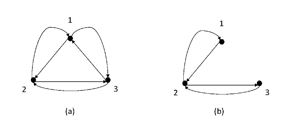
Two cases are considered. First, suppose the neighbor graph $\mathbb{N}(t)$ is fixed as shown in Figure 1(a). The system considered includes input white noise with zero mean, that is $\dot{x}=Ax+v$ where $E[v(t)]=0,E[v(t)v^{\prime}(s)]=0.5^{2}\delta(t-s)$ . With $g=10$ obtained using (30), the real part of the right most eigenvalue of $A_{V}$ is less than $-1$ . With randomly chosen initial state values, traces of this simulation are shown in Fig. 2(a) where $x_{i}^{1}$ and $x^{1}$ denote the first components of $x_{i}$ and $x$ respectively. Moreover, the norm of the estimation error is plotted in Fig. 2(b) from which we can see that it is exponentially convergent with the approximate rate $\lambda=1$ .

Second, suppose the neighbor graph $\mathbb{N}(t)$ is time-varying and switching back and forth between Figure 1(a) and Figure 1(b) according to the indicator function in Fig. 3. That is, when the function value is $1$ , the neighbor graph is Figure 1(a), and when the function value is $0$ , the neighbor graph is Figure 1(b). It is arranged that the average dwell time is $\tau_{D}=0.0369$ for this simulation. With zero measurement noise the corresponding solution trajectories for $x_{i}^{3}$ and $x^{1}$ are shown in Fig. 4(a) and the norm of the estimation error is shown in Fig. 4(b).

4.2 Discrete dynamics

The following simulations are intended to illustrate how to pick the integer parameter $q$ of the observer. Consider the three channel, four-dimensional, discrete-time system described by the equations $x(\tau+1)=Ax(\tau),\;y_{i}=C_{i}x,\;i\in\{1,\;2,\;3\}$ , where $A$ and $C_{i}$ are the same as described in §4.1. The observer convergence rate is designed to be $\lambda=0.5$ . The first step is also to design $K_{i}$ as stated in §3.1. For each agent $i$ , matrices $A_{i}$ , $Q_{i}$ , and $V_{i}$ remain the same as stated in §4.1.

For agent 1: $K_{1}=\begin{bmatrix}0.5&0.94&0&0\end{bmatrix}^{\prime}$

For agent 2: $K_{2}=\begin{bmatrix}-0.94&0.5&0&0\end{bmatrix}^{\prime}$

For agent 3: $K_{3}=\begin{bmatrix}0&0&0.5&1.94\end{bmatrix}^{\prime}$

Consider the case when the neighbor graph $\mathbb{N}$ is constant as in Fig. 1 (a). With randomly chosen initial state values and $q=6$ obtained using (59), which leads to a spectral radius of $\tilde{A}(V^{\prime}\bar{S}V)^{6}$ less than $0.5$ , the norm of the estimation error is plotted in Fig. 6(a) from which we can see that it is exponentially convergent with the rate $\lambda=0.5$ . The error traces are bounded by the curve $50\times 0.5^{\tau}$ .

Consider the case when the neighbor graph is switching between Fig. 1 (a) and (b) according to Fig. 5. The system considered has input white noise $v$ which satisfies $v\sim\mathcal{N}(0,0.1^{2})$ , that is $x(\tau+1)=Ax(\tau)+v$ . The norm of the estimation error is shown in Fig. 6(b) with the same value of $q$ .

5 Concluding Remarks

The distributed state estimation problem is studied when the neighbor graph is time-varying. It has been shown that, each agent can estimate the state exponentially fast with a pre-assigned convergence rate for both continuous-time and discrete-time systems.

The distributed state estimators developed in both §2 and §3 rely on an especially useful observation about distributed estimator structure first noted in [12] and subsequently exploited in [14] and [1]. That is to split the system spectrum into disjoint subsets corresponding to unobservable and observable subspaces. Just how much further this idea can be advanced remains to be seen. Generalization on the constraint of strong connectivity for the neighbor graph can be studied in future work. Certainly the synchronous switching upon which the local estimators in §3 depend can be relaxed by judicious application of the mixed matrix norm discussed here. This generalization will be addressed in future work.

Appendix A Proofs for Continuous-Time Distributed Estimator

Proof of Proposition 2: Recall $\bar{S}=S\otimes I_{n}$ . Since $S$ is a stochastic matrix, $S^{\prime}$ must have a spectral radius of $1$ and an eigenvalue at $1$ . Moreover, since $\mathbb{N}$ is the graph of $S^{\prime}$ and $\mathbb{N}$ is strongly connected by assumption, $S^{\prime}$ is irreducible {Theorem 6.2.24, [31]}. Thus by the Perron-Frobenius Theorem there must be a positive vector $\pi$ such that $S^{\prime}\pi=\pi$ . Without loss of generality, assume $\pi$ is normalized so that the sum of its entries equals $1$ ; i.e., $\pi$ is a Perron vector [31]. Let $\Pi$ be that diagonal matrix whose diagonal entries are the entries of $\pi$ . Then $\Pi\mathbf{1}=\pi$ where $\mathbf{1}$ is the $m$ -vector of all $1$ s. Let $L=2\Pi-\Pi S-S^{\prime}\Pi$ . Clearly $L$ is a symmetric matrix and $L\mathbf{1}=0$ .

We claim that the geometric multiplicity of $L$ ’s eigenvalue at $0$ is one. To establish this claim, note first that every nonzero entry of $S^{\prime}$ is a nonzero entry of $\Pi S+S^{\prime}\Pi$ because $S^{\prime}$ is a nonnegative matrix and $\Pi$ is a diagonal matrix whose diagonal entries are all positive. Moreover since $2(I_{m}-\Pi)$ is a nonnegative matrix, every nonzero entry of $S^{\prime}$ is also a nonzero entry of $2I_{m}-L=2(I_{m}-\Pi)+\Pi S+S^{\prime}\Pi$ . Thus the graph of $S^{\prime}$ must be a spanning subgraph of the graph of $2I_{m}-L$ so the graph of $2I_{m}-L$ must be strongly connected. Therefore $2I_{m}-L$ must be irreducible. Note that the row sums of $2I_{m}-L$ all equal $2$ . Since $2I_{m}-L$ is nonnegative, its infinity norm is $2$ so its spectral radius is no greater than $2$ {Theorem 5.6.9, [31]}. Moreover $2$ is an eigenvalue of $2I_{m}-L$ . Thus by the Perron-Frobenius Theorem, the geometric multiplicity of this eigenvalue is one. It follows that the geometric multiplicity of the eigenvalue of $L$ at $0$ is also one.

We claim that $L$ is positive semi-definite. To establish this claim, note that $L$ can also be written as $L=D-\widehat{A}$ where $D$ is a diagonal matrix whose entries are the diagonal entries of $L$ and $\widehat{A}$ is the nonnegative matrix $\widehat{A}=D-L$ . As such, $L$ is the generalized Laplacian [35] of that simple undirected graph $\mathbb{G}$ whose adjacency matrix is the matrix which results when the nonzero entries $a_{ij}$ in $\widehat{A}$ are replaced by ones. Since $L$ can also be written as

L=\sum_{(i,j)\in\mathcal{E}}a_{ij}(u_{i}-u_{j})(u_{i}-u_{j})^{\prime}

where $u_{i}$ is the $i$ th unit vector and $\mathcal{E}$ is the edge set of $\mathbb{G}$ , $L$ is positive semi-definite as claimed.

To proceed, set

H=\text{ block diag }\{\pi_{1}I_{n_{1}},\pi_{2}I_{n_{2}},\ldots,\pi_{m}I_{n_{m}}\}

(28)

where $n_{i}=\dim\mathcal{V}_{i}$ and note that $VH=(\Pi\otimes I_{n})V$ . Since $((S-I_{m})^{\prime}\otimes I_{n})(\Pi\otimes I_{n})=((S-I_{m})^{\prime}\Pi)\otimes I_{n}$ it must be true that $(V^{\prime}((S-I_{m})\otimes I_{n})V)^{\prime}H=V^{\prime}(((S-I_{m})^{\prime}\Pi)\otimes I_{n})V$ and thus that

		$\displaystyle\;H(V^{\prime}(I_{mn}-\bar{S})V)+(V^{\prime}(I_{mn}-\bar{S})V)^{\prime}H$
		$\displaystyle=V^{\prime}(L\otimes I_{n})V$		(29)

Observe that this is a Lyapunov equation for the positive definite function $z^{\prime}Hz$ . Therefore to show that $-V^{\prime}(I_{mn}-\bar{S})V$ is a stability matrix, it is enough to show that $V^{\prime}(L\otimes I_{n})V$ is positive definite.

Since $L$ is positive semi-definite, so must be $L\otimes I_{n}$ . Therefore $V^{\prime}(L\otimes I_{n})V$ is at least positive semi-definite. Suppose $z^{\prime}V^{\prime}(L\otimes I_{n})Vz=0$ where $z=$ col $\{z_{1},z_{2},\ldots,z_{m}\}$ and $z_{i}\in{\rm I\!R}^{\dim(\mathcal{V}_{i})}$ . To show that $V^{\prime}(L\otimes I_{n})V$ is positive definite, it is enough to show that $z=0$ . Since $L$ ’s eigenvalue at $0$ has multiplicity one, $\ker L=$ span $\{\mathbf{1}\}$ ; therefore $\ker(L\otimes I_{n})=$ column span $\mathbf{1}\otimes I_{n}$ . The hypothesis $z^{\prime}V^{\prime}(L\otimes I_{n})Vz=0$ implies that $(L\otimes I_{n})Vz=0$ so $Vz\in\ker(L\otimes I_{n})$ . Therefore $V_{i}z_{i}=V_{j}z_{j},\;i,j\in\mathbf{m}$ . But because of joint observability, $\bigcap_{i\in\mathbf{m}}\mathcal{V}_{i}=0$ so $V_{i}z_{i}=0,\;i\in\mathbf{m}$ . Thus $z_{i}=0,\;i\in\mathbf{m}$ so $z=0$ implying that $V^{\prime}(L\otimes I_{n})V$ is positive definite. Therefore $-V^{\prime}(I_{mn}-\bar{S})V$ is a continuous-time stability matrix as claimed.

Proof of Theorem 1: Recall that the state estimation error satisfied (4). The overall error dynamic is defined as (5). According to (11), the spectrum of $\bar{A}-gP(I_{mn}-\bar{S})$ is equivalent to the union of the spectrum of $\bar{A}_{V}$ and $A_{V}$ . Since the spectrum of $\bar{A}_{i}+\bar{K}_{i}\bar{C}_{i},\;i\in\mathbf{m}$ , is assignable with $\bar{K}_{i}$ , to show for $g$ sufficiently large that $\bar{A}-gP(I_{mn}-\bar{S})$ is a continuous-time stability matrix with a prescribed convergence rate as large as $\lambda$ , it is enough to show that for $g$ sufficiently large, the matrix $A_{V}=\tilde{A}-gV^{\prime}(I_{mn}-\bar{S})V$ is a continuous-time stability matrix with a prescribed convergence rate as large as $\lambda$ .

To show that $\text{exp}\{(\tilde{A}-gV^{\prime}((I_{m}-S)\otimes I_{n})V)t\}$ can be made to converge to zero as fast as $\text{exp}({-\lambda t})$ does by choosing $g$ sufficiently large, we exploit (29). Note in particular that

			$\displaystyle H(\lambda I+A_{V})+(\lambda I+A_{V})^{\prime}H$
		$\displaystyle=$	$\displaystyle H(\lambda I+\tilde{A})+(\lambda I+\tilde{A})^{\prime}H-gV^{\prime}(L\otimes I_{n})V$

Since $V^{\prime}(L\otimes I_{n})V$ is positive definite, by picking $g$ sufficiently large, $H(\lambda I+\tilde{A})+(\lambda I+\tilde{A})^{\prime}H-gV^{\prime}(L\otimes I_{n})V$ will be negative definite implying that $\lambda I+A_{V}$ is a stability matrix and thus that $\tilde{A}-gV^{\prime}(I_{mn}-\bar{S})V$ is a stability matrix for which $\text{exp}\{(\tilde{A}-gV^{\prime}(I_{mn}-\bar{S})V)t\}$ converges to zero as fast as $\text{exp}({-\lambda t})$ does. In other words, any value of $g$ will have the desired property provided

g\geq\frac{\lambda_{\max}\left(H(\lambda I+\tilde{A})+(\lambda I+\tilde{A})^{\prime}H\right)}{\lambda_{\min}\left(V^{\prime}(L\otimes I_{n})V\right)}

(30)

where $\lambda_{\max}(.)$ and $\lambda_{\min}(.)$ are the largest eigenvalue and the smallest eigenvalue of a symmetric matrix respectively.

Proof of Lemma 1: ⁵⁵ 5 The symbols used in this proof such as $g$ , $c$ and $\lambda^{*}$ are generic and do not have the same meanings as the same symbols do when used elsewhere in this paper. By hypothesis, each $M_{i}$ is exponentially stable. Thus there are positive constants $c_{i}>1$ and $\lambda_{i}$ such that

\|\text{exp}({M_{i}t})\|\leq c_{i}\text{exp}({-\lambda_{i}t})

(31)

for any $i\in\{1,2,\ldots,|\mathcal{G}|\}$ . Here $\|\cdot\|$ is any given submultiplicative norm on $\mathbb{R}^{n\times n}$ . Let

c=\max_{i\in\{1,2,\ldots,|\mathcal{G}|\}}c_{i},\;\text{and }\lambda^{*}=\min\limits_{i\in\{1,2,\ldots,|\mathcal{G}|\}}\lambda_{i}.

Fix $\lambda>0$ and let $g$ be any gain satisfying

g\geq\frac{\tau_{D}(\lambda+\|N\|c)+\ln c}{\tau_{D}\lambda^{*}}

(32)

We claim that for any number $\tau$ , and any switching signal $\sigma\in\mathcal{S}_{\text{avg}}$ , the transition matrix of $gM_{\sigma}$ , namely $\Phi_{\sigma}(t,\tau)$ , converges to zero as fast as $\text{exp}({-\alpha t})$ does where

\alpha=\lambda+\|N\|c

(33)

To understand why this is so, by (31),

\|\Phi_{\sigma}(t,\tau)\|\leq c^{\delta_{\sigma}(\tau,t)}\text{exp}({-g\lambda^{*}(t-\tau)})

(34)

where $\delta_{\sigma}(\tau,t)$ is the number of switching between $(\tau,t)$ . By (32), $\text{exp}({g\lambda^{*}})\geq c^{\frac{1}{\tau_{D}}}\text{exp}({\alpha})$ . From this and the fact that $\delta_{\sigma}(\tau,t)\leq\delta_{0}+\frac{t-\tau}{\tau_{D}}$ ,

\|\Phi_{\sigma}(t,\tau)\|\leq c^{\delta_{0}}c^{\frac{t-\tau}{\tau_{D}}}\text{exp}({-g\lambda^{*}(t-\tau)})\\ \leq c^{\delta_{0}-\frac{\tau}{\tau_{D}}}\text{exp}({-\alpha(t-\tau)}).

Thus, the claim is true.

In view of (12) and the variation of constants formula,

x(t)=\Phi_{\sigma}(t,0)x(0)+\int_{0}^{t}\Phi_{\sigma}(t,\mu)Nx(\mu)d\mu

(35)

As $\|\Phi_{\sigma}(t,\tau)\|\leq c\ \text{exp}({-\alpha t})$ for all $\tau$ and $\sigma\in\mathcal{S}_{\text{avg}}$ ,

\|x(t)\|\leq c\ \text{exp}({-\alpha t})\|x(0)\|+\\ \int_{0}^{t}c\ \text{exp}({-\alpha(t-\mu)})\|N\|\|x(\mu)\|d\mu

By multiplying by $\text{exp}({\alpha t})$ on both sides, one obtains $\text{exp}({\alpha t})\|x(t)\|\leq c\|x(0)\|+\int_{0}^{t}||N||c\ \text{exp}({\alpha\mu})\|x(\mu)\|d\mu$ . From this and the Bellman-Gronwall Lemma there follows

\text{exp}({\alpha t})\|x(t)\|\leq c\|x(0)\|\ \text{exp}({\int_{0}^{t}\|N\|cd\mu})

Since $\int_{0}^{t}\|N\|cd\mu=\|N\|ct$ , it follows that $\text{exp}({\alpha t})\|x(t)\|\leq c\|x(0)\|\text{exp}({\|N\|ct})$ and thus that

\|x(t)\|\leq c\|x(0)\|\text{exp}({(\|N\|c-\alpha)t})

From this and (33) it follows that

\|x(t)\|\leq c\|x(0)\|\text{exp}({-\lambda t})

This completes the proof.

Proof of Theorem 2: Recall that $A_{V}(t)=\tilde{A}-gV^{\prime}(I_{mn}-\bar{S}(t))V$ . By Proposition 2, for any fixed time $\tau$ , $-V^{\prime}(I_{mn}-\bar{S}(\tau))V$ is exponentially stable if the graph of $S(\tau)^{\prime}$ is strongly connected. Note $\tilde{A}$ is fixed and bounded. According to Lemma 1, for each $\sigma\in\mathcal{S}_{\text{avg}}$ there is a positive number $g$ , depending on $\tau_{D}$ so that the transition matrix of $A_{V}(t)$ converges to zero at least as fast as $\text{exp}({-\lambda t})$ does. This is accomplished by choosing $g$ sufficiently large. Based on the proof of Lemma 1, it is sufficient to pick $g$ to satisfy

g\geq\frac{\ln c+(\lambda+\|\tilde{A}\|c)\tau_{D}}{\lambda^{*}\tau_{D}}

(36)

where $c$ and $\lambda^{*}$ are two positive numbers chosen so that for any fixed $\tau$ , $\|\text{exp}\{-V^{\prime}(I_{mn}-\bar{S}(\tau))Vt\}\|\leq c\ \text{exp}({-\lambda^{*}t})$ , and $c>1$ . This completes the proof.

Proof of Theorem 3: Recall $\Phi_{V}(t,\tau)$ is the transition matrix of $A_{V}(t)$ for any $t\geq\tau\geq 0$ . If we can show that there exist a constant $c$ so that

\|\Phi_{V}(t,\tau)\|\leq c\ \text{exp}({-\lambda(t-\tau)}),\;\;\;\forall t\geq\tau\geq 0

the remaining proof is exactly the same as the proof of Theorem 1 which is omitted here.

It is left to show that $\|\Phi_{V}(t,\tau)\|\leq c\ \text{exp}({-\lambda(t-\tau)})$ for all $t\geq\tau\geq 0$ by choosing $g$ sufficiently large. We explore the matrix $A_{V}(t)$ . Recall that $A_{V}(t)=\tilde{A}-gV^{\prime}((I_{m}-S(t))\otimes I_{n})V$ . In particular,

			$\displaystyle(\lambda I+A_{V}(t))+(\lambda I+A_{V}(t))^{\prime}$
		$\displaystyle=$	$\displaystyle(\lambda I+\tilde{A})+(\lambda I+\tilde{A})^{\prime}$
			$\displaystyle-gV^{\prime}((2I_{m}-S(t)-S^{\prime}(t))\otimes I_{n})V$

Since each $S(t)$ is doubly stochastic, $2I_{m}-S(t)-S^{\prime}(t)$ has row sum $0$ , all its off-diagonal entries are non-positive, and all its diagonal entries are positive. That is, this matrix can be seen as a generalized Laplacian matrix of a connected graph. By Proposition 2, for any $t$ , $-V^{\prime}((2I_{m}-S(t)-S^{\prime}(t))\otimes I_{n})V=-V^{\prime}(I_{mn}-\bar{S}(t))V-V^{\prime}(I_{mn}-\bar{S}^{\prime}(t))V$ is negative definite. Thus by picking $g$ sufficiently large, $(\lambda I+A_{V}(t))+(\lambda I+A_{V}(t))^{\prime}$ will be negative definite for any time $t$ .

Consider system

\dot{\bar{z}}=A_{V}(t)\bar{z}

Let $V=\bar{z}^{\prime}\bar{z}$ . Then

\dot{V}=\bar{z}^{\prime}(A_{V}(t)^{\prime}+A_{V}(t))\bar{z}\leq-2\lambda\bar{z}^{\prime}\bar{z}

Therefore, $\Phi_{V}(t,\tau)$ converges to zero as fast as $\text{exp}({-\lambda(t-\tau)})$ does, i.e.,

\|\Phi_{V}(t,\tau)\|\leq c\ \text{exp}({-\lambda(t-\tau)}),\;\;\;\forall t\geq\tau\geq 0

This completes the proof.

Proof of Theorem 4: Equation (13) can be rewritten as

\dot{g}_{i}=|V_{i}^{\prime}W_{i}e|_{2}^{2},\;\;\;i\in\mathbf{m}

(37)

where $W_{i}=\begin{bmatrix}W_{i1}&\ldots&W_{im}\end{bmatrix}\in\mathbb{R}^{n\times nm}$ . Here $W_{ij}\in\mathbb{R}^{n\times n}$ is $\frac{1}{m_{i}}I_{n}$ if $j\neq i$ and $j\in\mathcal{N}_{i}$ , and $W_{ij}$ is $-I_{n}$ if $j=i$ . Otherwise $W_{ij}$ is a $0$ matrix. Let $\text{column}\{W_{1},W_{2},\ldots,W_{m}\}=W$ .

Different from (5), the error model turns to

\dot{e}=(\bar{A}-G(t)P(I_{mn}-\bar{S}(t))e

(38)

where $G(t)=\text{ block diag }\{g_{1}(t)I_{n},\ldots,g_{m}(t)I_{n}\}$ . Let $\begin{bmatrix}(Qe)^{\prime}&z^{\prime}\end{bmatrix}^{\prime}=T^{-1}e$ where $T=\begin{bmatrix}Q^{-1}&V\end{bmatrix}$ as defined earlier. Here $z=[z_{1}^{\prime},\ \ldots,z_{m}^{\prime}]^{\prime}$ iwth $z_{i}=V_{i}^{\prime}e_{i}$ .

Based on (11) and (38), the dynamic of $z_{i}$ can be written in the following form

\dot{z}_{i}=\tilde{A}_{i}z_{i}-g_{i}(t)V_{i}^{\prime}M_{i}e+\hat{A}_{i}Q_{i}e_{i},\;\;i\in\mathbf{m}

(39)

where $\tilde{A}_{i}=V_{i}^{\prime}(A+K_{i}C_{i})V_{i}$ , and $\hat{A}_{i}=V_{i}^{\prime}(A+K_{i}C_{i})Q_{i}^{\prime}$ .

First, we want to show that all $g_{i}(t)$ are bounded. We prove this by contradiction. Without generality, suppose that $g_{i}$ for $i\in\mathcal{V}_{u}=\{1,2,\ldots,m_{1}\}$ are unbounded, and $g_{i}$ for $i\in\mathcal{V}_{b}=\{m_{1}+1,m_{1}+2,\ldots,m\}$ are bounded where $\mathcal{V}_{u}\cap\mathcal{V}_{b}=0$ and $\mathcal{V}_{u}\cup\mathcal{V}_{b}=\mathbf{m}$ .

Let $R=R_{1}+R_{2}+R_{3}+R_{4}$ where the individual $R_{i}$ involve new positive parameters $p$ , $\alpha_{0}$ , $\alpha_{m_{1}+1},\dots,\alpha_{m}$ .

R_{1}=\frac{1}{2}\sum_{i=1}^{m_{1}}\pi_{i}\frac{p}{g_{i}(t)}|z_{i}|_{2}^{2},\;\;R_{2}=\frac{1}{2}\sum_{i=m_{1}+1}^{m}\pi_{i}\frac{g_{i}(0)}{g_{i}(t)}|z_{i}|_{2}^{2}

R_{3}=-\sum_{i=m_{1}+1}^{m}\alpha_{i}g_{i}(t),\text{and }R_{4}=-\alpha_{0}\int_{0}^{t}|Qe|_{2}^{2}dt.

The way to pick positive parameters $p$ , $\alpha_{0}$ , and $\alpha_{i}$ for $i\in\mathcal{V}_{b}$ is specified as follows.

Picking $p\geq 1$ :

Let $\mathcal{W}_{1}$ be a positive matrix matrix chosen such that

z^{\prime}\mathcal{W}_{1}z=\sum_{i=1}^{m}\pi_{i}|\tilde{A}_{i}|_{2}|z_{i}|_{2}^{2}

(40)

According to (29),

F=\frac{1}{2}(HV^{\prime}(\bar{S}-I_{mn})V+V^{\prime}(\bar{S}-I_{mn})^{\prime}VH)>0

(41)

Pick $p$ so that $\mathcal{W}_{2}=pF-\mathcal{W}_{1}>0$

Picking $\alpha_{0}$ , and $\alpha_{i}$ , $i\in\mathcal{V}_{b}$ :

Using the Cauchy-Schwarz inequality, the following three inequalities can be derived. For $\beta_{1}>0,\;\beta_{2}>0$ and $\lambda_{i}>0{\text{ for }}i\in\mathcal{V}_{b}$ , all for the moment otherwise arbitrary, write $\hat{A}=\text{block diag }\{\hat{A}_{1},\ldots,\hat{A}_{m}\}$

z^{\prime}H\hat{A}Qe\leq\frac{\beta_{1}}{2}|\hat{A}^{\prime}Hz|_{2}^{2}+\frac{1}{2\beta_{1}}|Qe|_{2}^{2},

(42)

-pz^{\prime}HV^{\prime}(\bar{S}-I_{mn})Q^{\prime}Qe\leq\\ \frac{\beta_{2}}{2}|Q(\bar{S}-I_{mn})^{\prime}VHz|_{2}^{2}+\frac{1}{2\beta_{2}}|Qe|_{2}^{2}

(43)

-\pi_{i}(g_{i}(0)-p)z_{i}^{\prime}V_{i}^{\prime}W_{i}e\leq\\ \frac{\lambda_{i}}{2}|\pi_{i}(g_{i}(0)-p)z_{i}|_{2}^{2}+\frac{1}{2\lambda_{i}}|V_{i}^{\prime}W_{i}e|_{2}^{2}.

(44)

Let $\mathcal{W}_{3}$ be a symmetric matrix chosen such that

	$\displaystyle z^{\prime}\mathcal{W}_{3}z$	$\displaystyle=$	$\displaystyle z^{\prime}\mathcal{W}_{2}z-\frac{\beta_{1}}{2}\|\hat{A}^{\prime}Hz\|_{2}^{2}-\frac{\beta_{2}}{2}\|Q(\bar{S}-I_{mn})^{\prime}VHz\|_{2}^{2}$		(45)
			$\displaystyle-\sum_{i=m_{1}+1}^{m}\frac{\lambda_{i}}{2}\|\pi_{i}(g_{i}(0)-p)z_{i}\|_{2}^{2}$		(45)

Pick positive $\beta_{1}$ , $\beta_{2}$ , and $\lambda_{i}$ for $i\in\mathcal{V}_{b}$ to be small enough so that $W_{3}$ is positive definite. Pick $\alpha_{0}$ and $\alpha_{i}$ , $i\in\mathcal{V}_{b}$ according to the following two equations:

\alpha_{0}=\frac{1}{2\beta_{1}}+\frac{1}{2\beta_{2}}\;\;\text{and }\;\;\alpha_{i}=\frac{1}{2\lambda_{i}}\;\;\;\;\;i\in\mathcal{V}_{b}

(46)

Now we consider the derivative of $R$ , i.e., $\dot{R}=\dot{R}_{1}+\dot{R}_{2}+\dot{R}_{3}+\dot{R}_{4}$ .

	$\displaystyle\dot{R}_{1}$	$\displaystyle=$	$\displaystyle-\frac{1}{2}\sum_{i=1}^{m_{1}}\pi_{i}\frac{p}{g_{i}^{2}}\|z_{i}\|_{2}^{2}\|V_{i}^{\prime}W_{i}e\|_{2}^{2}+\sum_{i=1}^{m_{1}}\pi_{i}\frac{p}{g_{i}}z_{i}^{\prime}\tilde{A}_{i}z_{i}$
			$\displaystyle+\sum_{i=1}^{m_{1}}\pi_{i}\frac{p}{g_{i}}z_{i}^{\prime}\hat{A}_{i}Q_{i}e_{i}-\sum_{i=1}^{m_{1}}\pi_{i}pz_{i}^{\prime}V_{i}^{\prime}W_{i}e$

Since for $i\in\mathcal{V}_{u}$ each $g_{i}(t)$ is unbounded, there is a time $T$ for $t\geq T$ , $p\leq g_{i}(t)$ for all $i\in\mathcal{V}_{u}$ . That is $\frac{p}{g_{i}(t)}\leq 1$ . Hence

\displaystyle\dot{R}_{1}\leq\sum_{i=1}^{m_{1}}\pi_{i}z_{i}^{\prime}\tilde{A}_{i}z_{i}+\sum_{i=1}^{m_{1}}\pi_{i}z_{i}^{\prime}\hat{A}_{i}Q_{i}e_{i}-\sum_{i=1}^{m_{1}}\pi_{i}pz_{i}^{\prime}V_{i}^{\prime}W_{i}e

(47)

According to (37), $g_{i}(t)$ is a non-decreasing function. As a result, $\frac{g_{i}(0)}{g_{i}(t)}\leq 1$ . Similar to the derivation of the inequality for $\dot{R}_{1}$ , it can be shown that

\dot{R}_{2}\!\!\leq\!\!\!\!\!\!\sum_{i=m_{1}+1}^{m}\!\!\!\!\!\!\pi_{i}z_{i}^{\prime}\tilde{A}_{i}z_{i}+\!\!\!\!\!\sum_{i=m_{1}+1}^{m}\!\!\!\!\!\pi_{i}z_{i}^{\prime}\hat{A}_{i}Q_{i}e_{i}-\!\!\!\!\!\sum_{i=m_{1}+1}^{m}\!\!\!\!\!\pi_{i}g_{i}(0)z_{i}^{\prime}V_{i}^{\prime}W_{i}e

(48)

By the submultiplicity of the matrix two norm, $z_{i}^{\prime}\tilde{A}_{i}z_{i}^{\prime}\leq|\tilde{A}_{i}|_{2}|z_{i}|_{2}^{2}$ . From this, (47), (48), (40) and (28),

$\displaystyle\dot{R}_{1}+\dot{R}_{2}$	$\displaystyle\leq$	$\displaystyle z^{\prime}\mathcal{W}_{1}z+\sum_{i=1}^{m}\pi_{i}z_{i}^{\prime}\hat{A}_{i}Q_{i}e_{i}-\sum_{i=1}^{m}\pi_{i}pz_{i}^{\prime}V_{i}^{\prime}W_{i}e$
		$\displaystyle-\sum_{i=m_{1}+1}^{m}\pi_{i}(g_{i}(0)-p)z_{i}^{\prime}V_{i}^{\prime}W_{i}e$
	$\displaystyle=$	$\displaystyle z^{\prime}\mathcal{W}_{1}z+z^{\prime}H\hat{A}Qe-pz^{\prime}HV^{\prime}(\bar{S}-I_{mn})e$
		$\displaystyle-\sum_{i=m_{1}+1}^{m}\pi_{i}(g_{i}(0)-p)z_{i}^{\prime}V_{i}^{\prime}W_{i}e$

It can be observed that $z^{\prime}HV^{\prime}(\bar{S}-I_{mn})e=z^{\prime}HV^{\prime}(\bar{S}-I_{mn})(VV^{\prime}e+Q^{\prime}Qe)=z^{\prime}HV^{\prime}(\bar{S}-I_{mn})Vz+z^{\prime}HV^{\prime}(\bar{S}-I_{mn})Q^{\prime}Qe$ . From this and (41), $z^{\prime}HV^{\prime}((S-I_{m})\otimes I_{n})e=z^{\prime}Fz+z^{\prime}HV^{\prime}((S-I_{m})\otimes I_{n})Q^{\prime}Qe$ . Thus

\dot{R}_{1}+\dot{R}_{2}\leq z^{\prime}(\mathcal{W}_{1}-pF)z+z^{\prime}H\hat{A}Qe-pz^{\prime}HV^{\prime}\\ (\bar{S}-I_{mn})Q^{\prime}Qe-\sum_{i=m_{1}+1}^{m}\pi_{i}(g_{i}(0)-p)z_{i}^{\prime}V_{i}^{\prime}W_{i}e\\ =-z^{\prime}\mathcal{W}_{2}z+z^{\prime}H\hat{A}Qe-pz^{\prime}HV^{\prime}\\ (\bar{S}\!-\!I_{mn}\!)Q^{\prime}Qe-\sum_{i=m_{1}+1}^{m}\pi_{i}(g_{i}(0)-p)z_{i}^{\prime}V_{i}^{\prime}W_{i}e

=-0.3in From this, (42), (43), and (44),

$\displaystyle\dot{R}_{1}+\dot{R}_{2}$	$\displaystyle\leq$	$\displaystyle-z^{\prime}\mathcal{W}_{2}z+\frac{\beta_{1}}{2}\|\hat{A}^{\prime}Hz\|_{2}^{2}+\frac{\beta_{2}}{2}\|Q(\bar{S}-I_{mn})^{\prime}VHz\|_{2}^{2}$	(49)
		$\displaystyle+\sum_{i=m_{1}+1}^{m}\frac{\lambda_{i}}{2}\|\pi_{i}(g_{i}(0)-p)z_{i}\|_{2}^{2}+\frac{1}{2\beta_{1}}\|Qe\|_{2}^{2}$
		$\displaystyle+\frac{1}{2\beta_{2}}\|Qe\|_{2}^{2}+\sum_{i=m_{1}+1}^{m}\frac{1}{2\lambda_{i}}\|V_{i}^{\prime}W_{i}e\|_{2}^{2}$

It is direct to get that

\dot{R}_{3}+\dot{R}_{4}=-\sum_{i=m_{1}+1}^{m}\alpha_{i}|V_{i}^{\prime}W_{i}e|_{2}^{2}-\alpha_{0}|Qe|_{2}^{2}

(50)

From (49), (50), and (46),

	$\displaystyle\dot{R}$	$\displaystyle\leq$	$\displaystyle-z^{\prime}\mathcal{W}_{2}z+\frac{\beta_{1}}{2}\|\hat{A}^{\prime}Hz\|_{2}^{2}+\frac{\beta_{2}}{2}\|Q((S-I)\otimes I)^{\prime}VHz\|_{2}^{2}$
			$\displaystyle+\sum_{i=m_{1}+1}^{m}\frac{\lambda_{i}}{2}\|\pi_{i}(g_{i}(0)-p)z_{i}\|_{2}^{2}$

According to (45),

\dot{R}\leq-z^{\prime}\mathcal{W}_{3}z<0

(51)

Since $Qe$ is exponentially convergent, the limit of $R_{4}(t)$ as $t$ goes to infinity exists. Due to the assumption that for $i\in\mathcal{V}_{b}$ , the $g_{i}$ are bounded. Thus $R_{3}$ is bounded. Therefore, $R$ is lower bounded. From this and (51) it follows that $z\in\mathcal{L}^{2}$ . From this and the fact that $Qe\in\mathcal{L}^{2}$ , we conclude $e\in\mathcal{L}^{2}$ . This with the definition of $\dot{g}_{i}$ imply that all $g_{i}$ for $i\in\mathbf{m}$ are bounded. Thus by contradiction all $g_{i}$ are bounded.

Next, we want to show that $e$ converges to zero. According to Theorem 1, let $G_{1}=g_{1}I$ be a matrix chosen so that $\bar{A}-G_{1}P(I_{mn}-\bar{S}(t))$ is a stable matrix. From (38), the dynamic of $e$ can be rewritten as

\dot{e}=(\bar{A}-G_{1}P(I_{mn}-\bar{S}(t)))e+(G_{1}-G)P(I_{mn}-\bar{S}(t))e

(52)

Since $(I_{mn}-\bar{S}(t))e\in\mathcal{L}^{2}$ , $G_{1}-G$ is bounded, and $\bar{A}-G_{1}P(I_{mn}-\bar{S}(t))$ is stable, thus $\dot{e}\in\mathcal{L}^{2}$ . Thus (52) is input-to-state stable which implies that $e$ must converge to zero asymptotically.

Appendix B Proofs for Discrete-Time Distributed Estimator

Proof of Lemma 2: Since $M$ is an $m\times m$ row stochastic matrix which ahs a strongly connected graph, $M$ is irreducible {Theorem 6.2.24, [31]}. Thus by the Perron-Frobenius Theorem there must be a positive vector $\pi$ such that $M^{\prime}\pi=\pi$ . Without loss of generality, assume $\pi$ is normalized so that the sum of its entries equals $1$ ; i.e., $\pi$ is a probability vector. Let $\Pi_{M}$ be that diagonal matrix whose diagonal entries are the entries of $\pi$ . Then $\Pi_{M}\mathbf{1}=\pi$ . Since $M\mathbf{1}=\mathbf{1}$ , $\Pi_{M}\mathbf{1}=\pi$ , and $M^{\prime}\pi=\pi$ , it must be true that $M^{\prime}\Pi_{M}M\mathbf{1}=\pi$ and thus that $L_{M}\mathbf{1}=0$ . Thus $L_{M}$ can also be written as $L_{M}=D-\hat{A}$ where $D$ is a diagonal matrix whose diagonal entries are the diagonal entries of $L_{M}$ and $\hat{A}$ is the nonnegative matrix $\hat{A}=D-L_{M}$ . Arguing as in the proof of Proposition 2, it can be shown that $L_{M}$ is positive-semidefinite.

Now suppose that the diagonal entries of $M$ are all positive. Then the diagonal entries of $M^{\prime}\Pi_{M}$ must also all be positive. It follows that every arc in the graph of $M^{\prime}$ must be an arc in the graph of $M^{\prime}\Pi_{M}M$ so the graph of $M^{\prime}\Pi_{M}M$ must be strongly connected. Since $I-\Pi_{M}$ is a nonnegative matrix, the graph of $M^{\prime}\Pi_{M}M$ must be a spanning subgraph of the graph of $I-\Pi_{M}+M^{\prime}\Pi_{M}M$ . Since $I-L_{M}=I-\Pi_{M}+M^{\prime}\Pi_{M}M$ and the graph of $M^{\prime}\Pi M$ is strongly connected, the graph of $I-L_{M}$ must be strongly connected as well. But $I-L_{M}$ is a nonnegative matrix so it must be irreducible. In addition, since $(I-L_{M})\mathbf{1}=\mathbf{1}$ , the row sums of $(I-L_{M})$ all equal one. Therefore the infinity norm of $I-L_{M}$ is one so its spectral radius is no greater than $1$ . Moreover $1$ is an eigenvalue of $I-L_{M}$ . Thus by the Perron-Frobenius Theorem, the geometric multiplicity of this eigenvalue is one. It follows that the geometric multiplicity of the eigenvalue of $L_{M}$ at $0$ is also one; ie, the dimension of the kernel of $L_{M}$ is one as claimed.

Proof of Proposition 4: Fix $\tau$ and write $S$ for $S(\tau)$ and $\bar{S}$ for $\bar{S}(\tau)$ . Note that the graph of $S^{\prime}$ , namely $\mathbb{N}$ , is strongly connected. In view of Lemma 2, the matrix $L=\Pi_{S}-S^{\prime}\Pi_{S}S$ is positive semi-definite and $L\mathbf{1}=0$ . Moreover, since the diagonal entries of $S$ and thus $S^{\prime}$ are all positive, the kernel of $L$ is one-dimensional.

Write $R$ for $R(\tau)$ . To prove the proposition it is enough to show that the matrix

Q=R-(V^{\prime}\bar{S}^{\prime}V)R(V^{\prime}\bar{S}V)

(53)

is positive definite.

To proceed, set $\bar{L}=L\otimes I_{n}$ in which case $\bar{L}$ is positive semi-definite because $L$ is. Moreover, $\bar{L}=\bar{\Pi}-\bar{S}^{\prime}\bar{\Pi}\bar{S}$ where $\bar{\Pi}=\Pi_{S}\otimes I_{n}$ . Note that $VRV^{\prime}=P\bar{\Pi}P$ where $P$ is the orthogonal projection matrix $P=VV^{\prime}$ . Clearly $VRV^{\prime}=P\bar{\Pi}^{\frac{1}{2}}\bar{\Pi}^{\frac{1}{2}}P$ . Note that both $P$ and $\bar{\Pi}^{\frac{1}{2}}$ are block diagonal matrices with corresponding diagonal blocks of the same size. Because of this and the fact that each diagonal block in $\bar{\Pi}^{\frac{1}{2}}$ is a scalar times the identity matrix, it must be true that $P$ and $\bar{\Pi}^{\frac{1}{2}}$ commute; thus $P\bar{\Pi}^{\frac{1}{2}}=\bar{\Pi}^{\frac{1}{2}}P$ . From this and the fact that $P$ is idempotent, it follows that $VRV^{\prime}=\bar{\Pi}^{\frac{1}{2}}P\bar{\Pi}^{\frac{1}{2}}$ . Clearly $\bar{\Pi}^{\frac{1}{2}}P\bar{\Pi}^{\frac{1}{2}}\leq\bar{\Pi}^{\frac{1}{2}}\bar{\Pi}^{\frac{1}{2}}$ so $VRV^{\prime}\leq\bar{\Pi}$ . It follows using (53) that $Q\geq R-V^{\prime}\bar{S}^{\prime}\bar{\Pi}\bar{S}V=R+V^{\prime}\bar{L}V-V^{\prime}\bar{\Pi}V$ . Therefore

Q\geq V^{\prime}\bar{L}V

(54)

In view of this, to complete the proof it is enough to show that $V^{\prime}\bar{L}V$ is positive definite. This can be shown by the same proof of Proposition 2.

Therefore $Q$ is positive definite because of (54). From this and (53) it follows that (27) is true.

Proof of Theorem 5: First it will be assumed that each $\bar{K}_{i}$ has been selected so that the the matrix $\bar{A}_{V}$ defined by (10), is such that $\bar{A}_{V}^{\tau}$ converges to zero as $\tau\rightarrow\infty$ as fast as $\lambda^{\tau}$ does. This can be done using standard spectrum assignment techniques to make the spectral radius of $\bar{A}_{V}$ at least as small as $\lambda$ . In view of (26), it is clear that to assign the convergence rate of the state transition matrix of $\bar{A}(I_{mn}-P(I_{mn}-\bar{S}(\tau)))^{q}$ it is necessary and sufficient to control the convergence rate of the state transition matrix of $A_{V}(\tau)$ . This, as we will now show, can be accomplished by choosing $q$ sufficiently large. We will actually detail two different ways to do this, each utilizing a different matrix norm. Both approaches will be explained next using the abbreviated notation $B(\tau)=V^{\prime}\bar{S}(\tau)V$ ; note that with this simplification, $A_{V}(\tau)=\tilde{A}B^{q}(\tau)$ because of (25).

Weighted Two-Norm: For each fixed $\tau$ and each appropriately-sized matrix $M$ , write $\|M\|_{R(\tau)}$ for the matrix norm induced by the vector norm $\|x\|_{R(\tau)}\stackrel{{\scriptstyle\Delta}}{{=}}\sqrt{x^{\prime}R(\tau)x}$ . Note that $\|M\|_{R(\tau)}$ is the largest singular value of $R^{\frac{1}{2}}(\tau)MR^{-\frac{1}{2}}(\tau)$ . Note in addition that

(R^{\frac{1}{2}}(\tau)B(\tau)R^{-\frac{1}{2}}(\tau))^{\prime}(R^{\frac{1}{2}}(\tau)B(\tau)R^{-\frac{1}{2}}(\tau))<I

because of (27). This shows that the largest singular value of $R^{\frac{1}{2}}(\tau)B(\tau)R^{-\frac{1}{2}}(\tau)$ is less than one. Therefore

\|B(\tau)\|_{R(\tau)}<1

(55)

a) $\mathbb{N}$ is constant

In this case both $B(\tau)$ and $R(\tau)$ are constant, so it is sufficient so choose choose $q$ so that $\|\tilde{A}B^{q}(\tau)\|_{R(\tau)}\leq\lambda$ . Since $\|\cdot\|_{R(\tau)}$ is submultiplicative, this can be done by choosing $q$ so that

\|B(\tau)\|^{q}_{R(\tau)}\leq\frac{\lambda}{\;\;\;\;\;\|\tilde{A}\|_{R(\tau)}}

(56)

This can always be accomplished because of (55).

b) $\mathbb{N}$ changes with time

In this case it is not possible to use the weighted two-norm $\|\cdot\|_{R(\tau)}$ because it is time-dependent. A simple fix, but perhaps not the most efficient one, would be to use the standard two-norm $|\cdot|_{2}$ instead since it does not depend on time. Using this approach, the first step would be to first choose, for each fixed $\tau$ , an integer $p_{1}(\tau)$ large enough so that $|B^{p_{1}(\tau)}(\tau)|_{2}<1$ . Such values of $p_{1}(\tau)$ must exist because each $B(\tau)$ is a discrete-time stability matrix or equivalently, a matrix with a spectral radius less than $1$ . Computing such a value amounts to looking at the largest singular value of $B^{p_{1}(\tau)}(\tau)$ for successively largest values of $p_{1}(\tau)$ until that singular value is less than $1$ . Having accomplished this, a number $p$ can easily be computed so that $|B^{p}(\tau)|_{2}<1\;\forall\tau$ since there are only a finite number of distinct strongly connected graphs on $m$ vertices and consequently only a finite number of distinct matrices $B(\tau)$ in the set $\mathcal{B}=\{B(\tau):\tau\geq 0\}$ . Choosing $p$ to be the maximum of the $p_{1}(\tau)$ with respect to $\tau$ is thus a finite computation. The next step would be to compute an integer $\bar{p}$ large enough so that each $|\tilde{A}(B^{p}(\tau))^{\bar{p}}|_{2}\leq\lambda$ . A value of $q$ with the required property would then be $q=p\bar{p}$ .

Mixed Matrix Norm: There is a different way to choose $q$ which does not make use of either Lemma 2 or Proposition 4. The approach exploits the “mixed matrix norm” introduced in [36]. To define this norm requires several steps. To begin, let $|\cdot|_{\infty}$ denote the standard induced infinity norm and write ${\rm I\!R}^{mn\times mn}$ for the vector space of all $m\times m$ block matrices $M=[M_{ij}]$ whose $ij$ th entry is a matrix $M_{ij}\in{\rm I\!R}^{n\times n}$ . With $n_{i}=\dim\mathcal{V}_{i},\;i\in\mathbf{m},$ and $\bar{n}=n_{1}+n_{2}+\cdots n_{m}$ , write ${\rm I\!R}^{mn\times\bar{n}}$ for the vector space of all $m\times m$ block matrices $M=[M_{ij}]$ whose $ij$ th entry is a matrix $M_{ij}\in{\rm I\!R}^{n\times n_{j}}$ . Similarly write ${\rm I\!R}^{\bar{n}\times mn}$ for the vector space of all $m\times m$ block matrices $M=[M_{ij}]$ whose $ij$ th entry is a matrix $M_{ij}\in{\rm I\!R}^{n_{i}\times n}$ . Finally write ${\rm I\!R}^{\bar{n}\times\bar{n}}$ for the vector space of all $m\times m$ block matrices $M=[M_{ij}]$ whose $ij$ th entry is a matrix $M_{ij}\in{\rm I\!R}^{n_{i}\times n_{j}}$ .

Note that $B\in{\rm I\!R}^{mn\times mn}$ , $\tilde{A}\in{\rm I\!R}^{\bar{n}\times\bar{n}}$ , $V\in{\rm I\!R}^{mn\times\bar{n}}$ , and $V^{\prime}\in{\rm I\!R}^{\bar{n}\times mn}$ . For $M$ in any one of these four spaces, the mixed matrix norm [36] of $M$ , written $\|M\|$ , is

\|M\|=\|\langle M\rangle\|_{\infty}

(57)

where $\langle M\rangle$ is the matrix in ${\rm I\!R}^{m\times m}$ whose $ij$ th entry is $\|M_{ij}\|_{2}$ . It is very easy to verify that $\|\cdot\|$ is in fact a norm. It is even sub-multiplicative whenever matrix multiplication is defined. Note in addition that $\|V\|=1$ and $\|V^{\prime}\|=1$ because the columns of each $V_{i}$ form an orthonormal set.

Recall that $P=VV^{\prime}$ is an orthogonal projection matrix. Using this, the definition of $B(\tau)$ and the fact that $PV=V$ , it is easy to see that for any integer $p>0$ , $B^{p}(\tau)=V^{\prime}(P\bar{S}(\tau)P)^{p}V$ . Thus $\|B^{p}(\tau)\|\leq\|(P\bar{S}(\tau)P)^{p}\|$ . Using this and the fact that the graph of $S^{\prime}$ is strongly connected, one can conclude that for $p\geq(m-1)^{2}$ , $\|(P\bar{S}(\tau)P)^{p}\|<1.$ This is a direct consequence of Proposition 2 of [36]. Thus

\|B^{p}(\tau)\|<1,\;\;\;p\geq(m-1)^{2}

(58)

a) $\mathbb{N}$ is constant

In this case $B(\tau)$ is constant so it is sufficient to choose $q$ so that $\|\tilde{A}B^{q}(\tau)\|\leq\lambda$ . This can be done by choosing $q=p\bar{p}$ where $p\geq(m-1)^{2}$ and $\bar{p}$ is such that

\|B^{p}(\tau)\|^{\bar{p}}\leq\frac{\lambda}{\|\tilde{A}\|}

(59)

This can always be accomplished because of (58).

b) $\mathbb{N}$ changes with time

Note that (58) holds for all $\tau$ . Assuming $p$ is chosen so that $p\geq(m-1)^{2}$ it is thus possible to find, for each $\tau$ , a positive integer $\bar{p}(\tau)$ , for which

\|B^{p}(\tau)\|^{\bar{p}(\tau)}\leq\frac{\lambda}{\|\tilde{A}\|}

(60)

Having accomplished this, a number $\bar{p}$ can easily be computed so that

\|B^{p}(\tau)\|^{\bar{p}}\leq\frac{\lambda}{\|\tilde{A}\|}

(61)

holds for all $\tau$ , since there there are only a finite number of distinct strongly connected graphs on $m$ vertices and consequently only a finite number of distinct matrices $B(\tau)$ in the set $\mathcal{B}$ defined earlier. Choosing $\bar{p}$ to be the maximum of $\bar{p}(\tau)$ with respect to $\tau$ is thus a finite computation. A value of $q$ with the required property would then be $q=p\bar{p}$ .

References

[1] L. Wang, J. Liu, and A. S. Morse. A distributed observer for a continuous-time linear system. In Proceedings of 2019 American Control Conference, pages 86–89, Philadelphia, PA, USA, July 2019.
[2] L. Wang, J. Liu, A. S. Morse, and B. D. O. Anderson. A Distributed Observer for a Discrete-Time Linear System. In Control and Decision conference, 2019.
[3] U. A. Khan and Ali Jadbabaie. On the stability and optimality of distributed Kalman filters with finite-time data fusion. In Proceedings of the 2011 American Control Conference, pages 3405–3410, 2011.
[4] R. Olfati-Reza and J. S. Shamma. Consensus filters for sensor networks and distributed sensor fusion. In Proc IEEE CDC, pages 6698–6703, 2005.
[5] L. Xiao, S. Boyd, and S. Lall. A scheme for robust distributed sensor fusion based on average consensus. In Proceedings of the 4th International Conference on Information Processing in Sensor Networks, pages 63–70, 2005.
[6] R. Olfati-Reza. Kalman-consensus filter: Optimality, stability, and performance. In Proc IEEE CDC, pages 7036–7042, 2009.
[7] F. Dorfler, F. Pasqualetti, and F. Bullo. Continuous-time distributed observers with discrete communication. IEEE Journal of Selected Topics in Signal Processing, 7(2):296–304, 2013.
[8] Y. Li, S. Phillips, and R. G. Sanfelice. Robust distributed estimationfor linear systems under intermittent information. IEEE Transactions on Automatic Control, 63(4):973–988, 2018.
[9] S. Park and N. C. Martins. Design of distributed LTI observers for state omniscience. IEEE Transactions on Automatic Control, pages 561–576, 2017.
[10] L. Wang and A. S. Morse. A distributed observer for an time-invariant linear system. IEEE Transactions on Automatic Control, 63(7):2123–2130, 2018.
[11] A. Mitra and S. Sundaram. Distributed observers for LTI systems. IEEE Transactions on Automatic Control, 63(11):3689–3704, 2018.
[12] T. Kim, H. Shim, and D. D. Cho. Distributed Luenberger observer design. In 2016 IEEE 55th Conference on Decision and Control (CDC), pages 6928–6933, Dec 2016.
[13] W. Han, H. L. Trentelman, Z. Wang, and Y. Shen. A simple approach to distributed observer design for linear systems. IEEE Transactions on Automatic Control, 64(1):329–336, 2019.
[14] W. Han, H. L. Trentelman, Z. Wang, and Y. Shen. Towards a minimal order distributed observer for linear systems. Systems and Control Letters, pages 59–65, 2018.
[15] L. Wang, A. S. Morse, D. Fullmer, and J. Liu. A hybrid observer for a distributed linear system with a changing neighbor graph. In Proceedings of the 2017 IEEE Conference on Decision and Control, pages 1024–1029, 2017.
[16] R. Olfati-Saber. Distributed Kalman filter with embedded consensus filters. Proceedings of the 44th IEEE Conference on Decision and Control, and the European Control Conference, CDC-ECC ’05, pages 8179–8184, 2005.
[17] R. Olfati-Saber. Distributed Kalman filtering for sensor networks. In Proceedings of the 46th IEEE Conference on Decision and Control, pages 5492–5498, 2007.
[18] L. Wang, A. S. Morse, and J. Liu. A hybrid observer for estimating the state of a distributed linear system. Automatica, 146:110633, 2022.
[19] L. Wang and A. S. Morse. A distributed observer for a time-invariant linear system. In Proceedings of the 2017 American Control Conference, pages 2020–2025, 2017.
[20] T. Kim, C. Lee, and H. Shim. Completely decentralized design of distributed observer for linear systems. IEEE Transactions on Automatic Control, 65(11):4664–4678, Nov 2020.
[21] J. G. Lee and H. Shim. A distributed algorithm that finds almost best possible estimate under non-vanishing and time-varying measurement noise. IEEE Control Systems Letters, 4(1):229–234, 2020.
[22] M. Doostmohammadian and U. A. Khan. On the genericity properties in distributed estimation: Topology design and sensor placement. IEEE Journal of Selected Topics in Signal Processing, 7(2):195–204, 2013.
[23] U. A. Khan and A. Jadbabaie. Collaborative scalar-gain estimators for potentially unstable social dynamics with limited communication. Autom., 50:1909–1914, 2014.
[24] S. Park and N. C. Martins. An augmented observer for the distributed estimation problem for LTI systems. In Proceedings the 2012 American Control Conference, pages 6775–6780, 2012.
[25] S. Park and N. C. Martins. Necessary and sufficient conditions for the stabilizability of a class of LTI distributed observers. In Proceedings of the 51st IEEE Conference on Decision and Control, pages 7431–7436, 2012.
[26] A. Mitra, J. A. Richards, S. Bagchi, and S. Sundaram. Finite-time distributed state estimation over time-varying graphs: Exploiting the age-of-information. 2019 American Control Conference (ACC), pages 4006–4011, 2019.
[27] B. Açikmeşe, M. Mandić, and J. L. Speyer. Decentralized observers with consensus filters for distributed discrete-time linear systems. Automatica, 50(4):1037–1052, 2014.
[28] V. A. Ugrinovskii. Distributed robust estimation over randomly switching networks using $h_{\infty}$ consensus. Automatica, 49:160–168, 2013.
[29] F. C. Rego, Y. Pu, A. Alessandretti, A. P. Aguiar, A. M. Pascoal, and C. N. Jones. A distributed Luenberger observer for linear state feedback systems with quantized and rate-limited communications. IEEE Transactions on Automatic Control, 66(9):3922–3937, 2021.
[30] A. Mitra, J. A. Richards, S. Bagchi, and S. Sundaram. Distributed state estimation over time-varying graphs: Exploiting the age-of-information. IEEE Transactions on Automatic Control, 67(12):6349–6365, 2022.
[31] R. A. Horn and C. R. Johnson. Matrix Analysis. Cambridge University Press, Cambridge, England, 1985.
[32] A. S. Morse. Dwell-time switching. In Proceedings of the 2nd European Control Conference, pages 176–181, 1993.
[33] J. P. Hespahna and A. S. Morse. Switched systems with average dwell time. In Proceedings of the IEEE Conference on Decision and Control, pages 2655–2660, 1999.
[34] B. D. O. Anderson and M. Gevers. Fundamental Problems in Adaptive Control, pages 9–21. Springer London, London, 1998.
[35] C. Godsil and G. Royle. Algebraic Graph Theory. Springer, 2001.
[36] S. Mou, J. Liu, and A. S. Morse. A distributed algorithm for solving a linear algebraic equation. IEEE Transactions on Automatic Control, 60(11):2863–2878, Nov 2015.

Split-Spectrum Based Distributed State Estimation for Linear Systemsfootnoteinfo

Abstract

keywords

1 Introduction

1.1 Background

2 Continuous-Time Distributed Estimator

2.1 The Estimator

2.1.1 The Error Dynamics

Proposition 1

2.2 Constant Neighbor Graph

Theorem 1

Proposition 2

2.3 Switching Neighbor Graph

Theorem 2

Lemma 1

Theorem 3

2.4 Distributed Estimator with Adaptive Gains

Theorem 4

2.5 Resilience

3 Discrete-Time Distributed Estimator

3.1 The Estimator

3.1.1 The Error Dynamics

Proposition 3

3.2 Time-varying Neighbor Graph

Theorem 5

Lemma 2

Proposition 4

Remark 1

4 Simulations

4.1 Continuous dynamics

4.2 Discrete dynamics

5 Concluding Remarks

Appendix A Proofs for Continuous-Time Distributed Estimator

Appendix B Proofs for Discrete-Time Distributed Estimator

References

Split-Spectrum Based Distributed State Estimation for Linear Systems^footnoteinfo