Pattern formation in odd viscoelastic fluids

Carlos Floyd Affiliation: The Chicago Center for Theoretical Chemistry, The University of Chicago, Chicago, Illinois 60637, USA Affiliation: Department of Chemistry, The University of Chicago, Chicago, Illinois 60637, USA Affiliation: The James Franck Institute, The University of Chicago, Chicago, Illinois 60637, USA Aaron R. Dinner Affiliation: The Chicago Center for Theoretical Chemistry, The University of Chicago, Chicago, Illinois 60637, USA Affiliation: Department of Chemistry, The University of Chicago, Chicago, Illinois 60637, USA Affiliation: The James Franck Institute, The University of Chicago, Chicago, Illinois 60637, USA Suriyanarayanan Vaikuntanathan Email: svaikunt@uchicago.edu Affiliation: The Chicago Center for Theoretical Chemistry, The University of Chicago, Chicago, Illinois 60637, USA Affiliation: Department of Chemistry, The University of Chicago, Chicago, Illinois 60637, USA Affiliation: The James Franck Institute, The University of Chicago, Chicago, Illinois 60637, USA

August 11, 2026

Abstract

Non-reciprocal interactions fueled by local energy consumption can be found in biological and synthetic active matter at scales where viscoelastic forces are important. Such systems can be described by “odd” viscoelasticity, which assumes fewer material symmetries than traditional theories. Here we study odd viscoelasticity analytically and using lattice Boltzmann simulations. We identify a pattern-forming instability which produces an oscillating array of fluid vortices, and we elucidate which features govern the growth rate, wavelength, and saturation of the vortices. Our observation of pattern formation through odd mechanical response can inform models of biological patterning and guide engineering of odd dynamics in soft active matter systems.

A striking feature of non-equilibrium systems is their tendency to undergo spatiotemporal pattern formation cross1993pattern; cross2009pattern. Coherent structures such as convective rolls busse1978non, Turing patterns turing1990chemical, and pulsatile contractions of active gels staddon2022pulsatile emerge spontaneously as the active driving in a system overcomes stabilizing dissipative forces. Pattern-forming instabilities are biologically important since, for example, they are utilized by growing organisms for morphogenesis gross2017active. In many biological examples of soft active matter systems, patterns are driven by the interplay of an active contribution to the local stress marchetti2013hydrodynamics; simha2002hydrodynamic; doostmohammadi2018active and a concentration field of chemical regulators bois2011pattern; kumar2014pulsatory; radszuweit2013intracellular; alonso2017mechanochemical; staddon2022pulsatile; del2022front. One can ask whether pattern formation in soft active matter systems can be reached through alternative routes which do not rely on active stresses and gradients of chemical regulators. We show here that pattern formation in a viscoelastic fluid can occur without either of these features, provided that the system displays odd non-equilibrium elastic responses to mechanical deformations.

Odd elasticity, which complements the older theory of odd viscosity avron1998odd; souslov2019topological; soni2019odd; han2021fluctuating; liao2019mechanism; hargus2020time; epstein2020time, has been developed by Vitelli and coworkers to describe elastic materials with internal energy-consuming degrees of freedom that do not obey several of the usual symmetries from classical elasticity theory scheibner2020odd; braverman2021topological; banerjee2021active; lier2022passive; fruchart2023odd. It has recently been reported that certain engineered and even biological systems exhibit odd elasticity: crystals of spinning magnetic colloids bililign2022motile and starfish embryos tan2022odd; certain active metamaterials chen2021realization; and even muscle fibers shankar2022active all transduce energy from an external or chemical drive into non-reciprocal pairwise interactions.

Whereas the predicted phenomenology of odd elastic systems, such as odd elastic waves and negative Poisson ratios scheibner2020odd; braverman2021topological, has been appreciably mapped out, the full implications of odd responses in viscoelastic materials remains to be explored. Some theoretical progress has been made in characterizing the thermodynamics and wave dispersion properties of odd viscoelastic materials scheibner2020odd; banerjee2021active; lier2022passive. These works identified novel transport properties and suggested ways that these properties could be experimentally detected; they also proposed that odd dynamics could be important for describing active biological materials like the actomyosin cortex. However, exploring this possibility for complex models which capture the composite nature of biological active matter requires advances in simulation methods to allow for tensorial viscoelastic responses in the hydrodynamic description of multi-component active viscoelastic fluids.

Here, we report on hydrodynamic simulations of a three-element active viscoelastic fluid using a recently developed extension of the hybrid lattice Boltzmann algorithm which can treat odd viscoelastic forces floyd2023simulating. Combining these simulations with linear instability analysis, we demonstrate that the interaction of passive viscosity and active odd elasticity allows for the emergence of an oscillating vortex array with a tunable characteristic wavelength and growth rate, a feature not observed in previous simplified models of odd viscoelasticity (Figure 1a). We additionally show that the initial exponential growth of the vortices saturates if a shear-thickening non-linearity is included in the dynamics. Our results suggest that such dynamical signatures may be generic to broad classes of odd viscoelastic systems encompassing various microscopic dynamics.

Refer to caption — Figure 1: Odd viscoelastic fluids. (a) Schematic illustration of the pattern formation instability observed in odd viscoelastic fluids. (b) A three-element mechanical circuit, comprising a viscous solvent in parallel with an odd Maxwell element, represents a minimal model for an odd viscoelastic fluid. (c) Two candidate systems which may display odd viscoelastic phenomenology.

Odd viscoelastic fluid model. Our model for odd viscoelasticity in this paper is an odd Jeffrey fluid. The usual Jeffrey fluid consists of a solvent phase in which a viscoelastic Maxwell material is immersed bird1987dynamics; larson2013constitutive, and it has been identified as a good description of biological systems like the cytoplasm Xiee2115593119; najafi2023size. In our case, while we treat the viscosities of the solvent and viscoelastic phases as scalar, we treat the elastic contribution to the fluid stress using the theory of odd elasticity. The mechanical circuit describing this viscoelastic model is depicted in Figure 1b. It can be shown that this model can map directly onto other three-element viscoelastic fluid models, such as one in which the solvent viscosity acts in series with a Kelvin-Voigt element; see Refs. 32; 35. We expect that an odd Jeffrey fluid could be physically realized in at least two types of systems: one in which active spinners are linked together through a polymer network howard2019structure, and one in which attractive interactions between the active spinners cause them to form a dense suspension through viscoelastic phase separation tanaka2000viscoelastic; patrick2008direct (Figure 1c). A key feature of these systems is that the spinners are not confined to a crystalline order, which would require description as an odd elastic or viscoelastic solid scheibner2020odd; bililign2022motile; tan2022odd; petroff2015fast.

The dynamical equations governing the evolution of the odd Jeffrey fluid are

$\displaystyle\partial_{t}\rho$	$\displaystyle=-\partial_{i}(\rho v_{i})$	(1)
$\displaystyle p$	$\displaystyle=c_{\text{s}}^{2}\rho$	(2)
$\displaystyle\rho D_{t}v_{i}$	$\displaystyle=-\partial_{i}p+2\eta_{\text{s}}\partial_{k}\Psi_{ik}+\partial_{k}\sigma_{ik}^{\text{p}}+f_{i}$	(3)
$\displaystyle\mathcal{D}_{t}\sigma_{ij}^{\text{p}}$	$\displaystyle=C_{ijkl}\partial_{k}v_{l}-\eta_{\text{p}}^{-1}C_{ijkl}\sigma_{kl}^{\text{p}}+D_{\text{p}}\partial_{kk}\sigma_{ij}^{\text{p}}.$	(4)

Here, $\rho$ is the fluid density, $\mathbf{v}$ is its velocity, $p$ is the pressure, $c_{\text{s}}$ is the speed of sound in the fluid, $\eta_{\text{s}}$ is the solvent’s dynamic viscosity, $\Psi_{ij}\equiv\left(\partial_{i}v_{j}+\partial_{j}v_{i}\right)/2$ is the symmetric strain rate tensor, and $\bm{\sigma}^{\text{p}}$ is the viscoelastic contribution to the stress tensor. The isothermal equation of state, Equation 2, implies that the fluid is weakly compressible kruger2017lattice; see Ref. 41 for recent work on the interplay of weak compressibility and odd viscous forces. The term $\mathbf{f}$ in the Navier-Stokes equation is an optional external force field. $\mathbf{C}$ is a rank four odd elasticity modulus tensor, $\eta_{\text{p}}$ is the dynamic viscosity of the viscoelastic phase (assumed to be scalar here), and $D_{\text{p}}$ is the viscoelastic stress diffusion constant olmsted2000johnson. Odd tensorial viscosity of the viscoelastic phase could be straightforwardly incorporated in this model by generalizing the coefficient $\eta_{\text{p}}^{-1}C_{ijkl}$ in Equation 4 as a rank four relaxation tensor $R_{ijkl}$ banerjee2021active. This would not affect the functional form of the model, so we omit this for simplicity. Further, $\partial_{t}$ is the partial derivative with respect to time, ${D_{t}\equiv\partial_{t}+v_{k}\partial_{k}}$ is the material derivative, and ${\mathcal{D}_{t}X_{ij}\equiv D_{t}X_{ij}+\Omega_{ik}X_{kj}-X_{ik}\Omega_{kj}}$ is the corotational derivative of the tensor $\mathbf{X}$ , with the vorticity tensor defined as ${\Omega_{ij}\equiv\left(\partial_{i}v_{j}-\partial_{j}v_{i}\right)}/2$ . If the upper convected derivative were used instead of the corotational derivative in Equation 4, we would have the Oldroyd-B model. In the subsequent linear instability calculation, however, these two derivatives are equivalent because they both reduce to $\partial_{t}$ to linear order, and our analytical results thus hold for the Oldroyd-B model as well.

In this work we consider an isotropic odd elastic modulus tensor $C_{ijkl}$ , whose form was derived in Ref. 22:

	$\displaystyle C_{ijkl}=$	$\displaystyle\ B\delta_{ij}\delta_{kl}+\mu\left(\delta_{il}\delta_{jk}+\delta_{ik}\delta_{jl}-\delta_{ij}\delta_{kl}\right)$
		$\displaystyle+K^{o}E_{ijkl}-A\epsilon_{ij}\delta_{kl},$		(5)

where $\delta_{ij}$ is the Kronecker delta, $\epsilon_{ij}$ is the Levi-Civita tensor, and $E_{ijkl}\equiv\left(\epsilon_{ik}\delta_{jl}+\epsilon_{il}\delta_{jk}+\epsilon_{jk}\delta_{il}+\epsilon_{jl}\delta_{ik}\right)/2$ . The bulk ( $B$ ) and shear ( $\mu$ ) moduli are found in classical elasticity theory, but the modulus $A$ , which transforms a dilatational deformation into torque (but not vice versa), and $K^{o}$ , which antisymmetrically couples the two shear modes, are the active “odd” moduli. Equation 4 is a phenomenological generalization of a standard Maxwell material to include odd elastic coefficients. It does not correspond to a specific microscopic system, instead serving as a general model to explore the repercussions of non-reciprocity in a composite viscoelastic material. In the Supplementary Methods, however, we illustrate how one can coarse-grain a microscopic “non-reciprocal elastic dumbbell” model to yield continuum equations with emergent odd coefficients like $K^{o}$ .

Results. The stability of the homogeneous state of the odd Jeffrey fluid is controlled by an intricate balance between stabilizing and destabilizing forces, the relative magnitudes of which depend on the parameters entering Equations 1-5. In Supplementary Methods Section IIA we derive the dispersion relation $\nu(k)$ for the growth of plane wave perturbations with the ansatz $e^{\nu(k)t}e^{i\mathbf{k}\cdot\mathbf{r}}$ for these dynamics. Linear instabilities occur when $\omega(k)>0$ for some wavenumber $k$ , where ${\omega(k)\equiv\text{max}_{n}\text{Re}[\nu_{n}(k)]}$ is the largest of the real part of nine branches of the dispersion relation $\nu(k)$ . The dispersion relation is complicated but reduces to the linear form derived in Ref. 43 in the special case ${\eta_{\text{s}}=0,\ \eta_{\text{p}}\rightarrow\infty,\ D_{\text{p}}=0}$ , and $A=0$ . Although the stabilizing forces in this composite viscoelastic fluid are more complex than those in a one-component viscoelastic solid as considered in Ref. 22, the intuition provided there of odd work cycles driving active waves also applies to understand the instabilities found in our model.

We studied how the various parameters control the system’s stability by plotting for each parameter the dispersion relation ${\omega_{\text{max}}\equiv\text{max}_{k}\omega(k)}$ over a range of parameter values (Figure 2a; see Supplementary Figure 1 for several other parameters). Key drivers of the instability include the odd moduli $A$ and $K^{o}$ : when their values lie outside a threshold set by the remaining parameters, the homogeneous state is unstable. Furthermore, $K^{o}$ alone is sufficient to cause instability, and $A$ cannot cause instability if $K^{o}=0$ . The two parameters work cooperatively if their signs agree, such that if $K^{o}>0$ then the instability growth rate increases as $A$ increases, but if $K^{o}<0$ the growth rate increases as $A$ decreases (Supplementary Figure 2). We also find that the value of the fastest growing wavenumber ${k_{\text{max}}\equiv\text{argmax}_{k}\omega(k)}$ increases with $K^{o}$ (Figure 2a and Supplementary Figure 4a) and either increases or decreases with $A$ depending on the relative signs of $K^{o}$ and $A$ .

The nature of the instability threshold qualitatively changes in the incompressible limit $c_{\text{s}}\rightarrow\infty$ (where dilatational deformations disappear, i.e., $\partial_{k}v_{k}=0$ ). First, as one might expect, the instability no longer depends on the moduli $A$ or $B$ which couple dilatational deformations to, respectively, a torque and an isotropic stress. Additionally, in the compressible case we typically observe two branches of the dispersion relation $\nu_{n}(k)$ which can take on real positive values for some $k$ . However, in the incompressible limit one of these branches shrinks below $0$ and remains stable for all $k$ (Figure 2b).

The shear modulus $\mu$ , the viscosities $\eta_{\text{s}}$ and $\eta_{\text{p}}$ , and the stress diffusion constant $D_{\text{p}}$ have predominantly stabilizing effects, causing $\omega(k)$ to decrease as their values increase (Figure 2c and Supplementary Figure 1). We note that $\eta_{\text{s}}$ is a key parameter which suppresses the linear relationship $\omega(k)\propto k$ at large $k$ (Supplementary Figure 3). This allows for a finite $k_{\text{max}}$ and thus a finite length scale of the instability. In previous work banerjee2021active $\eta_{\text{s}}$ was set to zero, precluding the observation of pattern formation since all wavelengths are unstable if $\omega(k)\propto k$ .

We next sought to study the growth of the instability in the compressible case using lattice Boltzmann simulations. To simulate an odd Jeffrey fluid, we apply a recently developed implementation of the hybrid lattice Boltzmann algorithm floyd2023simulating. To excite the instability in simulation we apply a short, periodic, random force $\mathbf{f}(\mathbf{r})$ (see Supplementary Methods Section IIB) and then evolve the system. As a readout of the instability, we use the total absolute vorticity in the system ${W\equiv\int|\Omega(\mathbf{r})|d\mathbf{r}}$ , where ${\Omega\equiv\partial_{x}v_{y}-\partial_{y}v_{x}=2\Omega_{xy}}$ . Above the instability threshold, $W$ oscillates and grows exponentially in time (Figure 3a). If the growth rate is fast enough that $W$ exceeds the value it attained during the initial perturbation in $0.2\ \text{s}$ , we conclude that the fluid is unstable. In Figure 3b we show that the conditions of $K^{o}$ and $\mu$ which are predicted to be unstable from the linear instability calculation are matched by those which produce a detected instability in simulation. In Supplementary Figure 4b we also show that the fastest growing wavelength of the instability matches the characteristic wavelength detected in simulation.

The spatial structure of the pattern is a regular periodic array of vortices with alternating handedness. The vorticity at a given point oscillates and grows exponentially in time, as shown in Figures 4a,b, where the vorticity at a point is fit to the functional form

\Omega(t)=a\exp(bt)\cos(ct+d).

(6)

We observe checkerboard and striped patterns as illustrated in Figure 4c,d and in Supplementary Figure 6. The periodic patterns do not travel but instead resemble standing waves. This instability falls in type $\text{I}_{\text{o}}$ of the classification of Cross and Hohenberg cross1993pattern, being periodic in space and oscillatory in time. Although we have focused on the vorticity $\Omega(\mathbf{r})$ as the pattern-forming field, we note that patterning appears for other fields as well, including the divergence, density, and torque, as shown in Supplementary Figure 7.

The initial exponential growth of the instability can in principle saturate due to various nonlinearities. The advective term in the Navier-Stokes equation, which is neglected for unsteady Stokes flows at low Reynolds number, is one possibility. We account for this term in our simulations, but we typically observe that the lattice Boltzmann algorithm becomes numerically unstable due to large fluid velocities before saturation from this term occurs. Another possible source is the nonlinear correction to the elastic forces experienced for large deformations, which we neglect here. Treating odd effects in the framework of finite elasticity requires additional theoretical development. Instead, we study here saturation caused by a shear-thickening nonlinearity which can result, for instance, from flocculation of dilatant viscoelastic suspensions like blood boersma1990shear; bodnar2009numerical. We consider a Carreau form carreau2021rheology $\eta_{\text{p}}(\Psi_{ij})=\eta_{\text{p}}^{0}\left(1+2\beta^{2}\Psi_{ij}\Psi_{ij}\right)^{(n-1)/2}$ which we use in Equation 4. The parameter $\beta$ sets the scale at which the shear flow $\Psi_{ij}$ begins to alter the viscosity, and the exponent $n$ determines if the system is shear-thinning ( $n<1$ ) or thickening ( $n>1$ ); here we use $n=1.5$ . In Supplementary Figure 5 we display the trajectory $W(t)$ for several values of $\beta$ , showing that this nonlinearity can significantly tune the flow rate in the pattern forming state of an odd viscoelastic fluid.

Conclusion. We have shown that “odd” moduli can provide a mechanism for pattern formation in non-equilibrium viscoelastic fluids. Whereas in typical soft active matter systems pattern formation is driven by active stresses and chemical regulators simha2002hydrodynamic; doostmohammadi2018active; bois2011pattern; kumar2014pulsatory; radszuweit2013intracellular; alonso2017mechanochemical; staddon2022pulsatile, here it is driven by active elastic response to mechanical deformations. Given that pattern formation and wave propagation due to active stresses can template developmental processes gross2017active, our discovery of another mechanism for pattern formation may have biological implications. Odd elastic forces could also interact with active stresses and chemical regulators. This may introduce new features to current models of traveling waves, pulsatile motions, and other dynamical patterns known to occur in biological or bio-inspired materials like actomyosin sheets bois2011pattern; staddon2022pulsatile; banerjee2017actomyosin; del2022front.

Collectives of rollers han2020emergence; han2020reconfigurable; zhang2022polar; han2023globally as well as both reconstituted and in vivo cytoskeletal systems tee2015cellular; schaller2010polar exhibit chiral and vortical flows similar to those reported here. While models for these systems are not currently framed using the theory of odd viscoelasticity, it should be possible to construct emergent, coarse-grained descriptions of their dynamics in terms of odd coefficients. In Supplementary Methods we provide an example of this type of coarse-graining for a microscopic “non-reciprocal elastic dumbbell” model; this derivation recapitulates the key coefficient $K^{o}$ driving instabilities in our phenomenological dynamical equations. We note that coarse-graining cytoskseletal systems poses a challenge that the constituent force dipoles are anisotropic, in contrast with the current isotropic model of odd elasticity.

We focused here on the linear instability of an odd Jeffrey fluid, but future work could clarify its rheological and dynamical properties. Detectable signatures of odd dynamics should be present even below the instability threshold. For example, we expect that in canonical setups such as Couette or Pouseille flow of a compressible odd Jeffrey fluid, one may find transverse components of the flow, analogous to the Hall effect. A recent theoretical study clarifies the expected dynamics experienced by a probe particle immersed in an odd viscoelastic fluid duclut2023probe. It would also be worth exploring whether features of pattern formation in other active systems such as screening by substrate friction doostmohammadi2016stabilization, wavelength selection by confinement chandrakar2020confinement, and transitions to turbulence wu2017transition; datta2022perspectives; de2023pattern occur in odd viscoelastic fluids.

Acknowledgments

We wish to thank Vincenzo Vitelli and his group for helpful discussions. This work was mainly supported by funds from DOE BES Grant DE-SC0019765 (CF and SV). ARD acknowledges support from the University of Chicago Materials Research Science and Engineering Center, which is funded by the National Science Foundation under award number DMR-2011854. CF acknowledges support from the University of Chicago through a Chicago Center for Theoretical Chemistry Fellowship. The authors acknowledge the University of Chicago’s Research Computing Center for computing resources.

I Supplementary Figures

II Supplementary Methods

II.1 Derivation of odd viscoelastic instability threshold

Here we derive the linear stability conditions for excitations in an odd viscoelastic fluid.

The dynamical equations governing the system are

$\displaystyle\partial_{t}\rho$	$\displaystyle=-\partial_{j}(\rho v_{j})$	(7)
$\displaystyle p$	$\displaystyle=c_{\text{s}}^{2}\rho$	(8)
$\displaystyle\rho D_{t}v_{i}$	$\displaystyle=-\partial_{i}p+\eta_{\text{s}}\partial_{j}\left(\partial_{j}v_{i}+\partial_{i}v_{j}\right)+\partial_{j}\sigma_{ij}^{\text{p}}$	(9)
$\displaystyle\mathcal{D}_{t}\sigma_{ij}^{\text{p}}$	$\displaystyle=C_{ijkl}\partial_{k}v_{l}-\eta_{\text{p}}^{-1}C_{ijkl}\sigma_{kl}^{\text{p}}+D_{\text{p}}\partial_{kk}\sigma_{ij}^{\text{p}}.$	(10)

See the main text for an explanation of the symbols in these equations. We have set the extra force density $\mathbf{f}$ to zero here.

In principle the viscous response of the viscoelastic phase may also require a tensorial description $\eta_{\text{p},ijkl}$ , causing the second term in Equation 10 to depend on a tensor formed from the elasticity and viscosity tensors banerjee2021active. This generalization would not change the form of the dispersion relation derived below, but would require reinterpreting certain coefficients. We leave this extension to future work. We also note that one can straightforwardly consider the incompressible case of these dynamics by substituting $p$ for $\rho$ using Equation 8 in Equations 7 and 9 and taking the limit $c_{\text{s}}\rightarrow\infty$ .

We first linearize the above equations around the uniform state $v^{u}_{i}=0,\ \rho^{u}=\rho_{\text{s}},\ \sigma^{u}_{ij}=0$ , such that $v_{i}=v_{i}^{\prime}\ \rho=\rho_{\text{s}}+\rho^{\prime}$ , and $\sigma_{ij}=\sigma^{\prime}_{ij}$ , where the primed variables are assumed small. The material and corotational derivatives reduce to partial derivatives to first order in the small variables. In what follows we drop the superscript p on the viscoelastic stress tensor, and we also drop the primes, with the understanding that all remaining variables are small. We eliminate the pressure from Equation 9 by substituting from Equation 8. The linearized set of equations is then

$\displaystyle\partial_{t}\rho$	$\displaystyle=-\rho_{\text{s}}\partial_{i}v_{i}$	(11)
$\displaystyle\rho_{\text{s}}\partial_{t}v_{i}$	$\displaystyle=-c_{\text{s}}^{2}\partial_{i}\rho+\eta_{\text{s}}\left(\partial_{jj}v_{i}+\partial_{j}\partial_{i}v_{j}\right)+\partial_{j}\sigma_{ij}$	(12)
$\displaystyle\partial_{t}\sigma_{ij}$	$\displaystyle=-\eta_{p}^{-1}C_{ijkl}\sigma_{kl}+C_{ijkl}\partial_{k}v_{l}+D_{\text{p}}\partial_{kk}\sigma_{ij}.$	(13)

Next we substitute the general form for the isotropic odd elastic tensor $C_{ijkl}$ , which is shown in Ref. 22 to be

C_{ijkl}=B\delta_{ij}\delta_{kl}+\mu\left(\delta_{il}\delta_{jk}+\delta_{ik}\delta_{jl}-\delta_{ij}\delta_{kl}\right)+K^{o}E_{ijkl}-A\epsilon_{ij}\delta_{kl}

(14)

where

E_{ijkl}=\frac{1}{2}\left(\epsilon_{ik}\delta_{jl}+\epsilon_{il}\delta_{jk}+\epsilon_{jk}\delta_{il}+\epsilon_{jl}\delta_{ik}\right).

(15)

Here $\delta_{ij}$ is the Kronecker delta and $\epsilon_{ij}$ is the Levi-Civita tensor. Note that the expression for $C_{ijkl}$ would be symmetric in the indices $i$ and $j$ if not for the term proportional to $A$ . With this, Equation 13 can be written as

$\displaystyle\partial_{t}\sigma_{ij}=$	$\displaystyle-\eta_{p}^{-1}\left((B-\mu)\delta_{ij}\sigma_{kk}+\mu\left(\sigma_{ij}+\sigma_{ji}\right)-A\epsilon_{ij}\sigma_{kk}+\frac{K^{o}}{2}\left(\epsilon_{ik}\sigma_{kj}+\epsilon_{il}\sigma_{jl}+\epsilon_{jk}\sigma_{ki}+\epsilon_{jl}\sigma_{il}\right)\right)$
	$\displaystyle+(B-\mu)\delta_{ij}\partial_{k}v_{k}+\mu\left(\partial_{j}v_{i}+\partial_{i}v_{j}\right)-A\epsilon_{ij}\partial_{k}v_{k}+\frac{K^{o}}{2}\left(\epsilon_{ik}\partial_{k}v_{j}+\partial_{j}\epsilon_{ik}v_{k}+\epsilon_{jk}\partial_{k}v_{i}+\partial_{i}\epsilon_{jk}v_{k}\right)$
	$\displaystyle+D_{\text{p}}\partial_{kk}\sigma_{ij}.$	(16)

We next change to the following variables:

$\displaystyle\Theta$	$\displaystyle\equiv\partial_{i}v_{i}$	(17)
$\displaystyle\Omega$	$\displaystyle\equiv\epsilon_{ij}\partial_{i}v_{j}$	(18)
$\displaystyle\sigma^{I}$	$\displaystyle\equiv\sigma_{ii}$	(19)
$\displaystyle\sigma^{II}$	$\displaystyle\equiv\partial_{i}\partial_{j}\sigma_{ij}$	(20)
$\displaystyle\sigma^{III}_{L}$	$\displaystyle\equiv\epsilon_{ik}\partial_{j}\partial_{k}\sigma_{ij}$	(21)
$\displaystyle\sigma^{III}_{R}$	$\displaystyle\equiv\epsilon_{jk}\partial_{i}\partial_{k}\sigma_{ij}.$	(22)

Our goal is now to express Equations 11, 12, and 13 in terms of these new variables. We divide this process into a few steps, as follows:

Take the time derivative of Equation 12. The result of this step is

\rho_{\text{s}}\partial_{t}^{2}v_{i}=-c_{\text{s}}^{2}\partial_{i}\partial_{t}\rho+\eta_{\text{s}}\partial_{t}\left(\partial_{jj}v_{i}+\partial_{j}\partial_{i}v_{j}\right)+\partial_{j}\partial_{t}\sigma_{ij}.

(23)

The expression for $\partial_{t}\sigma_{ij}$ can now be substituted from Equation 16.

Contract Equation 23 with $\partial_{i}$ This step produces an equation for the time evolution of $\Theta$ . After some algebra, we find

$\displaystyle\rho_{\text{s}}\partial_{t}^{2}\Theta=$	$\displaystyle-c_{\text{s}}^{2}\partial_{t}\nabla^{2}\rho+2\eta_{\text{s}}\partial_{t}\nabla^{2}\Theta$
	$\displaystyle-\eta_{\text{p}}^{-1}\left((B-\mu)\nabla^{2}\sigma^{I}+2\mu\sigma^{II}-K^{o}(\sigma^{III}_{R}+\sigma^{III}_{L})\right)$
	$\displaystyle+(B+\mu)\nabla^{2}\Theta+K^{o}\nabla^{2}\Omega+D_{\text{p}}\nabla^{2}\sigma^{II}.$	(24)

Contract Equation 23 with $\epsilon_{ki}\partial_{k}$ . This step produces an equation for the time evolution of $\Omega$ . We find

$\displaystyle\rho_{\text{s}}\partial_{t}^{2}\Omega=$	$\displaystyle\eta_{\text{s}}\partial_{t}\nabla^{2}\Omega$
	$\displaystyle+\eta_{\text{p}}^{-1}\left(\mu(\sigma_{L}^{III}+\sigma_{R}^{III})-A\nabla^{2}\sigma^{I}+K^{o}(2\sigma^{II}-\nabla^{2}\sigma^{I})\right)$
	$\displaystyle+\mu\nabla^{2}\Omega+A\nabla^{2}\Theta-K^{o}\nabla^{2}\Theta-D_{\text{p}}\nabla^{2}\sigma^{III}_{L}.$	(25)

4.

Contract Equation 16 with $\delta_{ij}$ . This step produces an equation for the time evolution of $\sigma^{I}$ . We find

$\displaystyle\partial_{t}\sigma^{I}=-\eta_{\text{p}}^{-1}(B+\mu)\sigma^{I}+(B+\mu)\Theta+D_{\text{p}}\nabla^{2}\sigma^{I}.$ (26)

Contract Equation 16 with $\partial_{i}\partial_{j}$ . This step produces an equation for the time evolution of $\sigma^{II}$ . We find

	$\displaystyle\partial_{t}\sigma^{II}=$	$\displaystyle-\eta_{\text{p}}^{-1}\left((B-\mu)\nabla^{2}\sigma^{I}+2\mu\sigma^{II}-K^{o}(\sigma_{L}^{III}+\sigma_{R}^{III})\right)$
		$\displaystyle+(B+\mu)\nabla^{2}\Theta+K^{o}\nabla^{2}\Omega+D_{\text{p}}\nabla^{2}\sigma^{II}.$		(27)

Contract Equation 16 with $\epsilon_{ik}\partial_{k}\partial_{j}$ . This step produces an equation for the time evolution of $\sigma^{III}_{L}$ . We find

	$\displaystyle\partial_{t}\sigma_{L}^{III}=$	$\displaystyle-\eta_{\text{p}}^{-1}\left(\mu(\sigma_{L}^{III}+\sigma_{R}^{III})-A\nabla^{2}\sigma^{I}+K^{o}(2\sigma^{II}-\nabla^{2}\sigma^{I})\right)$
		$\displaystyle-\mu\nabla^{2}\Omega-A\nabla^{2}\Theta+K^{o}\nabla^{2}\Theta+D_{\text{p}}\nabla^{2}\sigma_{L}^{III}.$		(28)

Contract Equation 16 with $\epsilon_{jk}\partial_{i}\partial_{k}$ . This step produces an equation for the time evolution of $\sigma^{III}_{R}$ . We find

	$\displaystyle\partial_{t}\sigma_{R}^{III}=$	$\displaystyle-\eta_{\text{p}}^{-1}\left(\mu(\sigma_{R}^{III}+\sigma_{L}^{III})+A\nabla^{2}\sigma^{I}+K^{o}(2\sigma^{II}-\nabla^{2}\sigma^{I})\right)$
		$\displaystyle-\mu\nabla^{2}\Omega+A\nabla^{2}\Theta+K^{o}\nabla^{2}\Theta+D_{\text{p}}\nabla^{2}\sigma_{R}^{III}.$		(29)

We now have a collection of 7 equations, including $\partial_{t}\rho=-\rho_{\text{s}}\Theta$ from Equation 11, in 7 variables. Next, we consider plane wave perturbations corresponding to the ansatz

\Theta(\mathbf{r},t)\sim\Theta(\mathbf{k},\omega)e^{\nu t}e^{i\mathbf{k}\cdot\mathbf{r}}

(30)

and convert the differential equations into algebraic equations in the Fourier coefficients. After this, we collect everything into the following matrix equation:

\begin{pmatrix}\nu&\rho_{\text{s}}&0&0&0&0&0\\ c_{\text{s}}^{2}k^{2}\nu&-k^{2}H_{+}-2k^{2}\eta_{\text{s}}\nu-\rho_{\text{s}}\nu^{2}&-k^{2}K^{o}&\frac{k^{2}H_{-}}{\eta_{\text{p}}}&-k^{2}D_{\text{p}}-\frac{2\mu}{\eta_{\text{p}}}&\frac{K^{o}}{\eta_{\text{p}}}&\frac{K^{o}}{\eta_{\text{p}}}\\ 0&-k^{2}G_{-}&-\rho_{\text{s}}\nu^{2}-k^{2}(\mu+\eta_{\text{s}}\nu)&\frac{k^{2}G_{+}}{\eta_{\text{p}}}&\frac{2K^{o}}{\eta_{\text{p}}}&D_{\text{p}}k^{2}+\frac{\mu}{\eta_{\text{p}}}&\frac{\mu}{\eta_{\text{p}}}\\ 0&H_{+}&0&-\frac{B+F_{1}}{\eta_{\text{p}}}&0&0&0\\ 0&-k^{2}H_{+}&-k^{2}K^{o}&\frac{k^{2}H_{-}}{\eta_{\text{p}}}&-\frac{F_{2}}{\eta_{\text{p}}}&\frac{K^{o}}{\eta_{\text{p}}}&\frac{K^{o}}{\eta_{\text{p}}}\\ 0&k^{2}G_{-}&k^{2}\mu&-\frac{k^{2}G_{+}}{\eta_{\text{p}}}&-\frac{2K^{o}}{\eta_{\text{p}}}&-\frac{F_{1}}{\eta_{\text{p}}}&-\frac{\mu}{\eta_{\text{p}}}\\ 0&-k^{2}G_{+}&k^{2}\mu&\frac{k^{2}G_{-}}{\eta_{\text{p}}}&-\frac{2K^{o}}{\eta_{\text{p}}}&-\frac{\mu}{\eta_{\text{p}}}&-\frac{F_{1}}{\eta_{\text{p}}}\\ \end{pmatrix}\begin{pmatrix}\rho\\ \Theta\\ \Omega\\ \sigma^{I}\\ \sigma^{II}\\ \sigma^{III}_{L}\\ \sigma^{III}_{R}\\ \end{pmatrix}=0,

(31)

where $F_{1}\equiv D_{\text{p}}k^{2}\eta_{\text{p}}+\mu+\eta_{\text{p}}\nu$ , $F_{2}\equiv D_{\text{p}}k^{2}\eta_{\text{p}}+2\mu+\eta_{\text{p}}\nu$ , $G_{\pm}\equiv A\pm K^{o}$ , and $H_{\pm}\equiv B\pm\mu$ .

Finally, the dispersion relation $\nu(k)$ is obtained as the solution of $\text{det}(\mathcal{M})=0$ , where $\mathcal{M}$ is the matrix in Equation 31. This equation has $9$ solutions which, without any further assumptions, are highly complicated. We do not write them here, but we note that they reduce to the results derived in Ref. 43 for the special case $\eta_{\text{s}}=0,\ \eta_{\text{p}}\rightarrow\infty,\ D_{\text{p}}=0$ , and $A=0$ .

II.2 Simulation methods

II.2.1 Numerical algorithm

To numerically solve the dynamical equations of the odd Jeffrey fluid, we rely on the hybrid lattice Boltzmann (HLB) method using the $d2Q9$ lattice carenza2019lattice. This technique uses a combination of the lattice Boltzmann method to update the velocity and density fields $\mathbf{v}(\mathbf{r})$ and $\rho(\mathbf{r})$ , and a finite difference integration scheme to update the polymer orientation vector field $\mathbf{P}(\mathbf{r})$ and the viscoelastic stress tensor field $\bm{\sigma}^{\text{p}}(\mathbf{r})$ . Periodic boundary conditions are used for all fields.

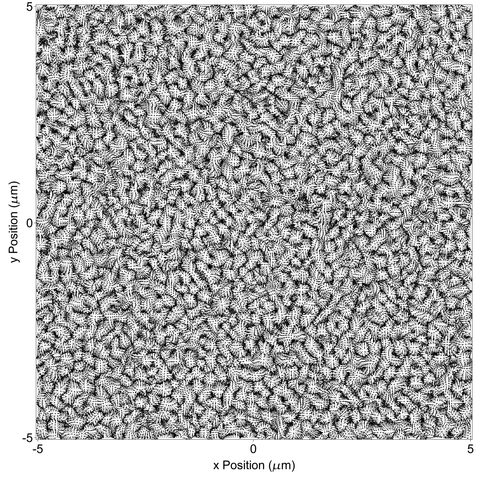
II.2.2 Initial perturbation

To numerically study pattern formation we apply a small initial perturbation to the fluid to excite the instability. This is done through the external body force field $\mathbf{f}_{\text{ext}}$ which is included as a contribution to the force density $\mathbf{f}$ in Equation 3 of the main text. Specifically, we apply a force of the form $\mathbf{f}_{\text{ext}}(\mathbf{r},t)=T(t)\mathbf{F}^{f}(\mathbf{r})$ , where $T(t)$ is a smooth bump function formed from sigmoidal curves that sets the magnitude of the force field, and $\mathbf{F}^{f}(\mathbf{r})$ is a normalized vector field. For the vector field, we use

	$\displaystyle F_{x}^{f}(x,y)=$	$\displaystyle\frac{1}{H}\sum_{i=1}^{N_{f}}\bigg(a^{\text{cx}}_{i}\cos(b^{\text{cx}}_{i}l_{x}x+c^{\text{cx}}_{i}l_{y}y)+a^{\text{sx}}_{i}\sin(b^{\text{sx}}_{i}l_{x}x+c^{\text{sx}}_{i}l_{y}y)\bigg)$		(32)
	$\displaystyle F_{y}^{f}(x,y)=$	$\displaystyle\frac{1}{H}\sum_{i=1}^{N_{f}}\bigg(a^{\text{cy}}_{i}\cos(b^{\text{cy}}_{i}l_{x}x+c^{\text{cy}}_{i}l_{y}y)+a^{\text{sy}}_{i}\sin(b^{\text{sy}}_{i}l_{x}x+c^{\text{sy}}_{i}l_{y}y)\bigg)$		(33)

where $l_{x}=2\pi/N_{x}$ and $l_{y}=2\pi/N_{y}$ . The random numbers $a^{\text{cx}}_{i},\ a^{\text{cy}}_{i},\ a^{\text{sx}}_{i}$ , and $a^{\text{sy}}_{i}$ are drawn from a normal distribution with mean $0$ and variance $1$ . The random numbers $b^{\text{cx}}_{i},\ c^{\text{cx}}_{i},\ b^{\text{sx}}_{i},\ c^{\text{sx}}_{i},\ b^{\text{cy}}_{i},\ c^{\text{cy}}_{i},\ b^{\text{sy}}_{i}$ , and $c^{\text{sy}}_{i}$ are drawn from a discrete uniform distribution over the domain $[-G,G]$ , with the integer $G$ chosen as $120$ for the grid size $N_{x}=N_{y}=750$ and $40$ for the grid size $N_{x}=N_{y}=250$ . We take $N_{f}=300$ and then normalize $\mathbf{F}^{f}(\mathbf{r})$ by choosing $H$ so that the largest vector in the field has unit norm. The magnitude $T^{f}(t)$ is kept at $10^{-8}$ (in lattice units) for the first $150$ timesteps of the simulation, with a sigmoidal width of $30$ timesteps.

The rationale behind this choice of perturbation is that it has the following desirable properties:

•

It is approximately isotropic, not preferring any direction in the grid.
•

When $G$ is large it allows for a wide range of spatial frequencies to be excited, increasing the chances that the fastest growing mode of the instability will be excited.
•

It obeys the periodic boundary conditions, avoiding a large gradient at the boundary due to a discontinuity.

An example of a vector field generated using this method is visualized in Figure 12.

II.2.3 Parameterization

Roughly, the system we have in mind is a micron-scale aqueous viscoelastic solution with elastic moduli on the order of a few Pa, corresponding to the cytoplasm. Experimentally verified parameter values, such as the viscosity of water, were used wherever possible. Several parameters were instead treated as free rather than constrained by experiments. The values reported in the tables below are the defaults, so when a given parameter is varied the remaining parameters are set to these values. We note that, following standard practice with LB simulations, the density of water is set to several orders of magnitude larger than its actual value tjhung2012spontaneous; cates2004simulating; wolff2012cytoplasmic; henrich2010ordering. This allows increasing the time step (thereby speeding up simulations) while still ensuring that the system has a small Reynolds number. We refer the reader to Ref. 31 for a full description of all parameters listed below.

Parameter	Symbol	Value
Lattice spacing	$\Delta x$	$4\times 10^{-8}$ m
Timestep	$\Delta t$	$8\times 10^{-6}$ s
Number of steps	$N_{\text{steps}}$	$25,000$ , $200,000$
Collision operator time	$\tau$	1.25
Solvent dynamic viscosity	$\eta_{\text{s}}$	0.001 Pa s
Solvent density	$\rho_{\text{s}}$	$2\times 10^{7}$ kg/m³
Lattice size	$N_{x}=N_{y}$	$250$ , $750$

Table 1: Default parameters used in simulation related to the LB algorithm and system domain are shown. These parameters were used to generate the data on the pattern forming instability.

Parameter	Symbol	Value
Polymeric viscosity	$\eta_{\text{p}}$	0.1 Pa s
Stress diffusion constant	$D_{\text{p}}$	$10^{-13}$ m²/s
Isotropic stiffness tensor element	$B$	5.0 Pa
Isotropic stiffness tensor element	$A$	5.0 Pa
Isotropic stiffness tensor element	$K^{o}$	5.0 Pa
Isotropic stiffness tensor element	$\mu$	2.0 Pa

Table 2: Default parameters used in simulation related to the viscoelastic stress are shown. These parameters were used to generate the data on the pattern forming instability.

II.2.4 Measuring the wavelength

To systematically estimate the length scale of the pattern as conditions are varied, we analyze the spatial correlation $C_{\Omega}(d)$ of the vorticity field $\Omega(\mathbf{r})$ . We first normalize $\Omega$ so that its maximum value over the grid is $1$ . We then estimate $C_{\Omega}(d)$ as

C_{\Omega}(d)=\frac{\sum_{i,j=1}^{N_{x},N_{y}}\delta(|i-j|-d)\left(\Omega_{ii}\Omega_{ij}+\Omega_{ii}\Omega_{ji}\right)}{2\sum_{i,j=1}^{N_{x},N_{y}}\delta(|i-j|-d)}

(34)

where $\delta(d)$ is the Kronecker delta function, and $\Omega_{ij}$ is value of $\Omega$ at the $i,j$ lattice point. This formula estimates $C_{\Omega}(d)$ by evaluating it for reference points along the main diagonal of the grid. The argument $d=r/\Delta x$ is in lattice units but can be converted to physical units using the simulation length scale $\Delta x$ .

For the periodic vortex arrays that make up the typical patterns observed in simulation, the correlation function $C_{\Omega}(d)$ is also roughly periodic (Figure 13). To estimate the wavelength of the array, we pick the value of $d$ where $C_{\Omega}(d)$ attains its first minimum. This value of $d$ is then interpreted as half of the pattern’s wavelength.

III A microscopic derivation of the viscoelastic dynamical equations

Here we consider a tractable microscopic system, a “non-reciprocal elastic dumbbell” model, and coarse-grain it following standard procedures to show how new “odd” terms emerge alongside those which appear in the usual upper-convected Maxwell model. This derivation does not reproduce the exact dynamical equations of the odd Jeffreys fluid considered in this paper, which requires a more detailed microscopic model and is left to future work. However, it does indicate how some new terms which are found in the odd Jeffreys dynamics arise from non-reciprocal interactions at the microscopic level.

Our derivation primarily follows Refs. 65 and 33, and we consider a 2D system. The standard elastic dumbbell model was introduced by Kuhn kuhn1934gestalt and describes a solution of polymers whose endpoints behave as if connected by a harmonic spring. The interactions between the polymer and the solvent are localized at these endpoints, which are at $\mathbf{r}_{+},\ \mathbf{r}_{-}$ and are governed by overdamped Langevin dynamics. The separation vector $\mathbf{R}\equiv\mathbf{r}_{+}-\mathbf{r}_{-}$ and center-of-mass position $\mathbf{R}^{c}=\frac{1}{2}(\mathbf{r}_{+}+\mathbf{r}_{-})$ obey, to second order in the solvent velocity $\mathbf{u}^{c}$ evaluated at $\mathbf{R}^{c}$ ,

\partial_{t}R_{i}^{c}=u_{i}^{c}+\frac{1}{8}R_{j}R_{k}\partial_{j}\partial_{k}u_{i}^{c}+\zeta^{-1}F^{b,c}_{i}(t),

(35)

\partial_{t}R_{i}=\left(\partial_{j}u^{c}_{i}\right)R_{j}+2\zeta^{-1}F_{i}^{\text{int}}+\zeta^{-1}F^{b}_{i}(t).

(36)

Here, $\zeta$ is a scalar friction coefficient obeying the fluctuation-dissipation relation with the Brownian forces $\mathbf{F}^{b,c}$ and $\mathbf{F}^{b}$ which act, respectively, on $\mathbf{R}^{c}$ and $\mathbf{R}$ :

\left\langle F_{i}^{b,c}(t)\right\rangle=0,\ \ \ \left\langle F_{i}^{b,c}(t+t^{\prime})F_{j}^{b,c}(t)\right\rangle=k_{B}T\zeta\delta(t^{\prime})\delta_{ij},

(37)

\left\langle F_{i}^{b}(t)\right\rangle=0,\ \ \ \left\langle F_{i}^{b}(t+t^{\prime})F_{j}^{b}(t)\right\rangle=4k_{B}T\zeta\delta(t^{\prime})\delta_{ij}.

(38)

In the standard elastic dumbbell model, the interaction force is

F_{i}^{\text{int}}=-k_{\parallel}R_{i},

(39)

i.e., the polymer behaves like a harmonic spring with zero rest length. We add to this interaction a transverse force depending on the separation $\mathbf{R}$ :

F_{i}^{\text{int}}=-k_{\parallel}R_{i}-k_{\perp}\epsilon_{ij}R_{j}=-M_{ij}R_{j},

(40)

where

M_{ij}=k_{\parallel}\delta_{ij}+k_{\perp}\epsilon_{ij}.

(41)

We seek the evolution of the quantity $\left\langle R_{i}R_{j}\right\rangle$ , which we will eventually relate to the viscoelastic stress tensor $\sigma_{ij}^{\text{p}}$ . Using Equation 36, we have

\partial_{t}(R_{i}R_{j})=\left(\partial_{k}u_{i}^{c}\right)R_{k}R_{j}+R_{i}R_{k}\left(\partial_{k}u^{c}_{j}\right)+2\zeta^{-1}\left(F^{\text{int}}_{i}R_{j}+F^{\text{int}}_{j}R_{i}\right)+\zeta^{-1}\left(F_{i}^{b}(t)R_{j}+F_{j}^{b}(t)R_{i}\right).

(42)

In expectation, the Brownian force terms can be simplified using a separation of timescales between $R_{i}$ and $F_{i}^{b}(t)$ phan2013understanding:

\left\langle R_{i}F_{j}^{b}\right\rangle\approx\left\langle F_{i}^{b}R_{j}\right\rangle\approx 2k_{B}T\delta_{ij}.

(43)

The interaction terms can be expressed as

F^{\text{int}}_{i}R_{j}+F^{\text{int}}_{j}R_{i}=-M_{ik}R_{k}R_{j}-R_{i}M_{jk}R_{k}=-\widetilde{C}_{ijkl}R_{k}R_{l}

(44)

where

	$\displaystyle\widetilde{C}_{ijkl}=$	$\displaystyle M_{ik}\delta_{jl}+M_{jk}\delta_{il}$		(45)
	$\displaystyle=$	$\displaystyle k_{\parallel}\left(\delta_{ik}\delta_{jl}+\delta_{jk}\delta_{il}\right)+\frac{k_{\perp}}{2}\left(\epsilon_{ik}\delta_{jl}+\epsilon_{il}\delta_{jk}+\epsilon_{jk}\delta_{il}+\epsilon_{jl}\delta_{ik}\right).$		(46)

This tensor is of the same form as Equation 14 above, when $B=\mu$ and $A=0$ . We note that the symmetrized combinations $(\epsilon_{ik}\delta_{jl}+\epsilon_{il}\delta_{jk})/2$ and $(\epsilon_{jk}\delta_{il}+\epsilon_{jl}\delta_{ik})/2$ appear because the contraction with $R_{k}R_{l}$ should be symmetric under the interchange of indices $k$ and $l$ . The expectation of Equation 42 can now be written as

\partial_{t}\left\langle R_{i}R_{j}\right\rangle=\left(\partial_{k}u_{i}^{c}\right)\left\langle R_{k}R_{j}\right\rangle+\left\langle R_{i}R_{k}\right\rangle\left(\partial_{k}u^{c}_{j}\right)-2\zeta^{-1}\widetilde{C}_{ijkl}\left\langle R_{k}R_{l}\right\rangle+4k_{B}T\zeta^{-1}\delta_{ij}.

(47)

The polymer-contributed stress can be written as $S^{\text{p}}_{ij}=(1/2)\nu\widetilde{C}_{ijkl}\left\langle R_{k}R_{l}\right\rangle$ where $\nu$ is the number density of polymers. Contracting both sides of Equation 47 with $\nu\widetilde{C}_{ijkl}$ and using the upper convected derivative $\mathcal{D}_{t}^{\text{uc}}X_{ij}=\partial_{t}X_{ij}-\left(\partial_{k}u_{i}^{c}\right)X_{kj}-X_{ik}\left(\partial_{k}u^{c}_{j}\right)$ , we have

\nu\widetilde{C}_{ijkl}\mathcal{D}_{t}^{\text{uc}}\left\langle R_{k}R_{l}\right\rangle=-4\zeta^{-1}\widetilde{C}_{ijkl}S^{\text{p}}_{kl}+4k_{B}T\nu\zeta^{-1}\widetilde{C}_{ijkl}\delta_{kl}.

(48)

The operations of $\mathcal{D}^{\text{uc}}_{t}$ and contraction with $\widetilde{C}_{ijkl}$ do not commute when $k_{\perp}\neq 0$ . However, since we are interested in the linear stability regime, for simplicity, we neglect the commutator of these operations, which is second order in the perturbations around the homogeneous state. It is standard to redefine the polymer stress to absorb the pressure-like term: $\sigma_{ij}^{\text{p}}=S_{ij}^{\text{p}}-k_{B}T\nu\delta_{ij}$ . With this, we can write

\mathcal{D}^{\text{uc}}_{t}S_{ij}^{\text{p}}=\mathcal{D}^{\text{uc}}_{t}\sigma_{ij}^{\text{p}}+k_{B}T\nu\mathcal{D}^{\text{uc}}_{t}\delta_{ij}=-2\zeta^{-1}\widetilde{C}_{ijkl}\sigma_{kl}^{\text{p}}.

(49)

One can show that $\mathcal{D}^{\text{uc}}_{t}\delta_{ij}=-\left(\partial_{i}u_{j}^{c}+\partial_{j}u_{i}^{c}\right)=-2\Psi_{ij}$ , so that

\mathcal{D}^{\text{uc}}_{t}\sigma_{ij}^{\text{p}}=2k_{B}T\nu\Psi_{ij}-2\zeta^{-1}\widetilde{C}_{ijkl}\sigma_{kl}^{\text{p}}.

(50)

If $k_{\perp}=0$ , then Equation 50 reduces to the standard upper convected Maxwell model:

\mathcal{D}_{t}^{\text{uc}}\sigma_{ij}^{\text{p}}=2k_{B}T\nu\Psi_{ij}-4k_{\parallel}\zeta^{-1}\sigma_{ij}^{\text{p}}.

(51)

Defining the relaxation time $\lambda=\zeta/4k_{\parallel}$ and thermal energy density $G=\nu k_{B}T$ , this can be expressed in the familiar form

\lambda\mathcal{D}_{t}^{\text{uc}}\sigma_{ij}^{\text{p}}=2\widetilde{\eta}_{\text{p}}\Psi_{ij}+\sigma_{ij}^{\text{p}}

(52)

where $\widetilde{\eta}_{\text{p}}=G\lambda$ . If the polymeric elasticity is due to the Kuhn stiffness of a Gaussian chain, we can write

k_{\parallel}=ak_{B}T,

(53)

where the proportionality $a$ (having units of inverse length squared) is related to the Kuhn length and the number of Kuhn segments. By assuming a similar relationship between stiffness $\widetilde{C}_{ijkl}$ and thermal energy for the case when $k_{\perp}\neq 0$ , we generalize the coefficient of $\Psi_{ij}$ in Equation 50 so that it reads

\mathcal{D}_{t}^{\text{uc}}\sigma_{ij}^{\text{p}}=\frac{2\nu}{a}\widetilde{C}_{ijkl}\Psi_{ij}-2\zeta^{-1}\widetilde{C}_{ijkl}\sigma_{kl}^{\text{p}}.

(54)

Defining $C_{ijkl}=\frac{2\nu}{a}\widetilde{C}_{ijkl}$ and $\eta_{\text{p}}=\zeta\nu/a$ , we can write

\mathcal{D}_{t}^{\text{uc}}\sigma_{ij}^{\text{p}}=C_{ijkl}\Psi_{ij}-\eta_{\text{p}}^{-1}C_{ijkl}\sigma_{kl}^{\text{p}}.

(55)

This last equation can be compared to Equation 10, and $\sigma_{ij}^{\text{p}}$ can be added to the solvent phase stresses to give the final Navier-Stokes equation for the Oldroyd-B fluid. An Oldroyd-B fluid, which is the same as a Jeffrey fluid but with an upper-convected rather than co-rotational derivative in the evolution for the viscoelastic stress tensor, is a model for a viscoelastic Maxwell material immersed in a viscous solvent. The two components are assumed to flow together, and thus one velocity field suffices to describe the motion of the combined system. The two components however make separate additive contributions to the total stress tensor, which enters the momentum-balance encoded in the Navier-Stokes equation. This physical approximation to the two-component system of polymer and solvent is quite standard in rheology, and models like the Jeffrey fluid have successfully reproduced numerous experimental observations phan2013understanding; bird1987dynamics; larson2013constitutive. We note that in certain situations this model suffers from physically inconsistent singularities owing to the assumed infinite extensibility of the constituent polymers. For our linear instability calculations this issue is not important.

The derivation presented here does not exactly reproduce Equation 10, missing some terms in the elasticity tensor and using a different materially objective derivative, but it illustrates how the odd coefficient $K^{o}$ in the elasticity tensor, which drives instabilities, arises from microscopic forces proportional to $k_{\perp}$ . Future work could focus on a similar derivation of viscoelastic dynamics from spinning colloids, rather than from a polymeric system with transverse forces as considered here.

References

[1] Mark C Cross and Pierre C Hohenberg. Pattern formation outside of equilibrium. Reviews of Modern Physics, 65(3):851, 1993.
[2] Michael Cross and Henry Greenside. Pattern formation and dynamics in nonequilibrium systems. Cambridge University Press, 2009.
[3] FH Busse. Non-linear properties of thermal convection. Reports on Progress in Physics, 41(12):1929, 1978.
[4] Alan Mathison Turing. The chemical basis of morphogenesis. Bulletin of mathematical biology, 52(1-2):153–197, 1990.
[5] Michael F Staddon, Edwin M Munro, and Shiladitya Banerjee. Pulsatile contractions and pattern formation in excitable actomyosin cortex. PLoS Computational Biology, 18(3):e1009981, 2022.
[6] Peter Gross, K Vijay Kumar, and Stephan W Grill. How active mechanics and regulatory biochemistry combine to form patterns in development. Annual review of biophysics, 46:337–356, 2017.
[7] M Cristina Marchetti, Jean-François Joanny, Sriram Ramaswamy, Tanniemola B Liverpool, Jacques Prost, Madan Rao, and R Aditi Simha. Hydrodynamics of soft active matter. Reviews of Modern Physics, 85(3):1143, 2013.
[8] R Aditi Simha and Sriram Ramaswamy. Hydrodynamic fluctuations and instabilities in ordered suspensions of self-propelled particles. Physical Review Letters, 89(5):058101, 2002.
[9] Amin Doostmohammadi, Jordi Ignés-Mullol, Julia M Yeomans, and Francesc Sagués. Active nematics. Nature communications, 9(1):3246, 2018.
[10] Justin S Bois, Frank Jülicher, and Stephan W Grill. Pattern formation in active fluids. Physical Review Letters, 106(2):028103, 2011.
[11] K Vijay Kumar, Justin S Bois, Frank Jülicher, and Stephan W Grill. Pulsatory patterns in active fluids. Physical Review Letters, 112(20):208101, 2014.
[12] Markus Radszuweit, Sergio Alonso, Harald Engel, and Markus Bär. Intracellular mechanochemical waves in an active poroelastic model. Physical Review Letters, 110(13):138102, 2013.
[13] Sergio Alonso, Markus Radszuweit, Harald Engel, and Markus Bär. Mechanochemical pattern formation in simple models of active viscoelastic fluids and solids. Journal of Physics D: Applied Physics, 50(43):434004, 2017.
[14] Clara Del Junco, André Estevez-Torres, and Ananyo Maitra. Front speed and pattern selection of a propagating chemical front in an active fluid. Physical Review E, 105(1):014602, 2022.
[15] JE Avron. Odd viscosity. Journal of Statistical Physics, 92(3):543–557, 1998.
[16] Anton Souslov, Kinjal Dasbiswas, Michel Fruchart, Suriyanarayanan Vaikuntanathan, and Vincenzo Vitelli. Topological waves in fluids with odd viscosity. Physical Review Letters, 122(12):128001, 2019.
[17] Vishal Soni, Ephraim S Bililign, Sofia Magkiriadou, Stefano Sacanna, Denis Bartolo, Michael J Shelley, and William Irvine. The odd free surface flows of a colloidal chiral fluid. Nature Physics, 15(11):1188–1194, 2019.
[18] Ming Han, Michel Fruchart, Colin Scheibner, Suriyanarayanan Vaikuntanathan, Juan J De Pablo, and Vincenzo Vitelli. Fluctuating hydrodynamics of chiral active fluids. Nature Physics, 17(11):1260–1269, 2021.
[19] Zhenghan Liao, Ming Han, Michel Fruchart, Vincenzo Vitelli, and Suriyanarayanan Vaikuntanathan. A mechanism for anomalous transport in chiral active liquids. Journal of Chemical Physics, 151(19):194108, 2019.
[20] Cory Hargus, Katherine Klymko, Jeffrey M Epstein, and Kranthi K Mandadapu. Time reversal symmetry breaking and odd viscosity in active fluids: Green-Kubo and NEMD results. Journal of Chemical Physics, 152(20):201102, 2020.
[21] Jeffrey M Epstein and Kranthi K Mandadapu. Time-reversal symmetry breaking in two-dimensional nonequilibrium viscous fluids. Physical Review E, 101(5):052614, 2020.
[22] Colin Scheibner, Anton Souslov, Debarghya Banerjee, Piotr Surówka, William Irvine, and Vincenzo Vitelli. Odd elasticity. Nature Physics, 16(4):475–480, 2020.
[23] Lara Braverman, Colin Scheibner, Bryan VanSaders, and Vincenzo Vitelli. Topological defects in solids with odd elasticity. Physical Review Letters, 127(26):268001, 2021.
[24] Debarghya Banerjee, Vincenzo Vitelli, Frank Jülicher, and Piotr Surówka. Active viscoelasticity of odd materials. Physical Review Letters, 126(13):138001, 2021.
[25] Ruben Lier, Jay Armas, Stefano Bo, Charlie Duclut, Frank Jülicher, and Piotr Surówka. Passive odd viscoelasticity. Physical Review E, 105(5):054607, 2022.
[26] Michel Fruchart, Colin Scheibner, and Vincenzo Vitelli. Odd viscosity and odd elasticity. Annual Review of Condensed Matter Physics, 14:471–510, 2023.
[27] Ephraim S Bililign, Florencio Balboa Usabiaga, Yehuda A Ganan, Alexis Poncet, Vishal Soni, Sofia Magkiriadou, Michael J Shelley, Denis Bartolo, and William Irvine. Motile dislocations knead odd crystals into whorls. Nature Physics, 18(2):212–218, 2022.
[28] Tzer Han Tan, Alexander Mietke, Junang Li, Yuchao Chen, Hugh Higinbotham, Peter J Foster, Shreyas Gokhale, Jörn Dunkel, and Nikta Fakhri. Odd dynamics of living chiral crystals. Nature, 607(7918):287–293, 2022.
[29] Yangyang Chen, Xiaopeng Li, Colin Scheibner, Vincenzo Vitelli, and Guoliang Huang. Realization of active metamaterials with odd micropolar elasticity. Nature communications, 12(1):1–12, 2021.
[30] Suraj Shankar and L Mahadevan. Active muscular hydraulics. bioRxiv, 2022.
[31] Carlos Floyd, Suriyanarayanan Vaikuntanathan, and Aaron R Dinner. Simulating structured fluids with tensorial viscoelasticity. Journal of Chemical Physics, 158(5):054906, 2023.
[32] Robert Byron Bird, Robert Calvin Armstrong, and Ole Hassager. Dynamics of Polymeric Liquids. Vol. 1: Fluid Mechanics. John Wiley and Sons Inc., New York, NY, 1987.
[33] Ronald G Larson. Constitutive Equations for Polymer Melts and Solutions. Butterworth-Heinemann, 2013.
[34] Jing Xie, Javad Najafi, Rémi Le Borgne, Jean-Marc Verbavatz, Catherine Durieu, Jeremy Sallé, and Nicolas Minc. Contribution of cytoplasm viscoelastic properties to mitotic spindle positioning. Proceedings of the National Academy of Sciences, 119(8), 2022.
[35] Javad Najafi, Serge Dmitrieff, and Nicolas Minc. Size-and position-dependent cytoplasm viscoelasticity through hydrodynamic interactions with the cell surface. Proceedings of the National Academy of Sciences, 120(9):e2216839120, 2023.
[36] Michael P Howard, Ryan B Jadrich, Beth A Lindquist, Fardin Khabaz, Roger T Bonnecaze, Delia J Milliron, and Thomas M Truskett. Structure and phase behavior of polymer-linked colloidal gels. Journal of Chemical Physics, 151(12):124901, 2019.
[37] Hajime Tanaka. Viscoelastic phase separation. Journal of Physics: Condensed Matter, 12(15):R207, 2000.
[38] C Patrick Royall, Stephen R Williams, Takehiro Ohtsuka, and Hajime Tanaka. Direct observation of a local structural mechanism for dynamic arrest. Nature materials, 7(7):556–561, 2008.
[39] Alexander P Petroff, Xiao-Lun Wu, and Albert Libchaber. Fast-moving bacteria self-organize into active two-dimensional crystals of rotating cells. Physical Review Letters, 114(15):158102, 2015.
[40] Timm Krüger, Halim Kusumaatmaja, Alexandr Kuzmin, Orest Shardt, Goncalo Silva, and Erlend Magnus Viggen. The lattice Boltzmann method. Springer International Publishing, 10(978-3):4–15, 2017.
[41] Ruben Lier, Charlie Duclut, Stefano Bo, Jay Armas, Frank Jülicher, and Piotr Surówka. Lift force in odd compressible fluids. Physical Review E, 108(2):L023101, 2023.
[42] PD Olmsted, O Radulescu, and C-YD Lu. Johnson–Segalman model with a diffusion term in cylindrical couette flow. Journal of Rheology, 44(2):257–275, 2000.
[43] Shiladitya Banerjee, Margaret L Gardel, and Ulrich S Schwarz. The actin cytoskeleton as an active adaptive material. Annual Review of Condensed Matter Physics, 11:421–439, 2020.
[44] Willem H Boersma, Jozua Laven, and Hans N Stein. Shear thickening (dilatancy) in concentrated dispersions. AIChE journal, 36(3):321–332, 1990.
[45] T Bodnár, A Sequeira, and L Pirkl. Numerical simulations of blood flow in a stenosed vessel under different flow rates using a generalized oldroyd-b model. In AIP Conference Proceedings, volume 1168, pages 645–648. American Institute of Physics, 2009.
[46] Pierre J Carreau, Daniel CR De Kee, and Raj P Chhabra. Rheology of Polymeric Systems: Principles and Applications. Carl Hanser Verlag GmbH Co KG, 2021.
[47] Deb Sankar Banerjee, Akankshi Munjal, Thomas Lecuit, and Madan Rao. Actomyosin pulsation and flows in an active elastomer with turnover and network remodeling. Nature communications, 8(1):1121, 2017.
[48] Koohee Han, Gašper Kokot, Oleh Tovkach, Andreas Glatz, Igor S Aranson, and Alexey Snezhko. Emergence of self-organized multivortex states in flocks of active rollers. Proceedings of the National Academy of Sciences, 117(18):9706–9711, 2020.
[49] Koohee Han, Gašper Kokot, Shibananda Das, Roland G Winkler, Gerhard Gompper, and Alexey Snezhko. Reconfigurable structure and tunable transport in synchronized active spinner materials. Science advances, 6(12):eaaz8535, 2020.
[50] Bo Zhang, Hang Yuan, Andrey Sokolov, Monica Olvera de la Cruz, and Alexey Snezhko. Polar state reversal in active fluids. Nature Physics, 18(2):154–159, 2022.
[51] Koohee Han, Andreas Glatz, and Alexey Snezhko. Globally correlated states and control of vortex lattices in active roller fluids. Physical Review Research, 5(2):023040, 2023.
[52] Yee Han Tee, Tom Shemesh, Visalatchi Thiagarajan, Rizal Fajar Hariadi, Karen L Anderson, Christopher Page, Niels Volkmann, Dorit Hanein, Sivaraj Sivaramakrishnan, Michael M Kozlov, et al. Cellular chirality arising from the self-organization of the actin cytoskeleton. Nature cell biology, 17(4):445–457, 2015.
[53] Volker Schaller, Christoph Weber, Christine Semmrich, Erwin Frey, and Andreas R Bausch. Polar patterns of driven filaments. Nature, 467(7311):73–77, 2010.
[54] Charlie Duclut, Stefano Bo, Ruben Lier, Jay Armas, Piotr Surówka, and Frank Jülicher. Probe particles in odd active viscoelastic fluids: how activity and dissipation determine linear stability. arXiv preprint arXiv:2310.08640, 2023.
[55] Amin Doostmohammadi, Michael F Adamer, Sumesh P Thampi, and Julia M Yeomans. Stabilization of active matter by flow-vortex lattices and defect ordering. Nature Communications, 7(10557):1–9, 2016.
[56] Pooja Chandrakar, Minu Varghese, S Ali Aghvami, Aparna Baskaran, Zvonimir Dogic, and Guillaume Duclos. Confinement controls the bend instability of three-dimensional active liquid crystals. Physical Review Letters, 125(25):257801, 2020.
[57] Kun-Ta Wu, Jean Bernard Hishamunda, Daniel TN Chen, Stephen J DeCamp, Ya-Wen Chang, Alberto Fernández-Nieves, Seth Fraden, and Zvonimir Dogic. Transition from turbulent to coherent flows in confined three-dimensional active fluids. Science, 355(6331):eaal1979, 2017.
[58] Sujit S Datta, Arezoo M Ardekani, Paulo E Arratia, Antony N Beris, Irmgard Bischofberger, Gareth H McKinley, Jens G Eggers, J Esteban López-Aguilar, Suzanne M Fielding, Anna Frishman, et al. Perspectives on viscoelastic flow instabilities and elastic turbulence. Physical Review Fluids, 7(8):080701, 2022.
[59] Xander M de Wit, Michel Fruchart, Tali Khain, Federico Toschi, and Vincenzo Vitelli. Pattern formation by non-dissipative arrest of turbulent cascades. arXiv preprint arXiv:2304.10444, 2023.
[60] Livio Nicola Carenza, Giuseppe Gonnella, Antonio Lamura, Giuseppe Negro, and Adriano Tiribocchi. Lattice Boltzmann methods and active fluids. The European Physical Journal E, 42(6):1–38, 2019.
[61] Elsen Tjhung, Davide Marenduzzo, and Michael E Cates. Spontaneous symmetry breaking in active droplets provides a generic route to motility. Proceedings of the National Academy of Sciences, 109(31):12381–12386, 2012.
[62] ME Cates, K Stratford, R Adhikari, P Stansell, JC Desplat, I Pagonabarraga, and AJ Wagner. Simulating colloid hydrodynamics with lattice Boltzmann methods. Journal of Physics: Condensed Matter, 16(38):S3903, 2004.
[63] K Wolff, D Marenduzzo, and ME Cates. Cytoplasmic streaming in plant cells: the role of wall slip. Journal of the Royal Society Interface, 9(71):1398–1408, 2012.
[64] Oliver Henrich, Kevin Stratford, Davide Marenduzzo, and Michael E Cates. Ordering dynamics of blue phases entails kinetic stabilization of amorphous networks. Proceedings of the National Academy of Sciences, 107(30):13212–13215, 2010.
[65] Nhan Phan-Thien and Nam Mai-Duy. Understanding viscoelasticity: an introduction to rheology. Springer, 2013.
[66] Werner Kuhn. Über die gestalt fadenförmiger moleküle in lösungen. Kolloid-Zeitschrift, 68:2–15, 1934.