An Analysis of RF Transfer Learning Behavior
Using Synthetic Data
Abstract
Transfer learning techniques, which leverage prior knowledge gained from data with different distributions to achieve higher performance and reduced training time, are often used in computer vision and natural language processing, but have yet to be fully utilized in the field of radio frequency machine learning. This work systematically evaluates how radio frequency transfer learning behavior by examining how the training domain and task, characterized by the transmitter/receiver hardware and channel environment, impact radio frequency transfer learning performance for an example automatic modulation classification use-case. Through exhaustive experimentation using carefully curated synthetic datasets with varying signal types, signal-to-noise ratios, and frequency offsets, generalized conclusions are drawn regarding how best to use radio frequency transfer learning techniques for domain adaptation and sequential learning. Consistent with trends identified in other modalities, results show that radio frequency transfer learning performance is highly dependent on the similarity between the source and target domains/tasks. Results also discuss the impacts of channel environment, hardware variations, and domain/task difficulty on radio frequency transfer learning performance, and compare radio frequency transfer learning performance using head re-training and model fine-tuning methods.
keywords
machine learning, deep learning, transfer learning, radio frequency machine learning2 Bradley Department of Electrical and Computer Engineering, Virginia Tech
3 Intel AI Lab, Santa Clara, CA††corresponding: Correspondence: ljwong@vt.edu††reftitle: References
1 Introduction
Radio frequency machine learning (RFML) is loosely defined as the application of deep learning to raw radio frequency data, and has yielded state-of-the-art algorithms for spectrum awareness, cognitive radio, and networking tasks. Existing radio frequency machine learning works have delivered increased performance and flexibility, and reduced the need for pre-processing and expert-defined feature extraction techniques. As a result, radio frequency machine learning is expected to enable greater efficiency, lower latency, and better spectrum efficiency in 6G systems Morocho-Cayamcela et al. 2019. However, to date, little research has considered and evaluated the performance of these algorithms in the presence of changing hardware platforms and channel environments, adversarial contexts, or resource constraints that are likely to be encountered in real-world systems Wong et al. 2021.


Current state-of-the-art radio frequency machine learning techniques rely upon supervised learning techniques trained from random initialization, and thereby assume the availability of a large corpus of labeled training data (synthetic, captured, or augmented Clark IV et al. 2021), which is representative of the anticipated deployed environment. Over time, this assumption inevitably breaks down as a result of changing hardware and channel conditions, and as a consequence, performance degrades significantly Hauser 2018; Sankhe et al. 2019. Transfer learning techniques can be used to mitigate these performance degradations by using prior knowledge obtained from a source domain and task, in the form of learned representations, to improve performance on a “similar” target domain and task using less data, as depicted in Fig. 1.

Though transfer learning techniques have demonstrated significant benefits in fields such as computer vision and natural language processing Ruder 2019, including higher performing models, significantly less training time, and far fewer training samples Olivas et al. 2009, Wong and Michaels 2022 showed that the use of transfer learning in radio frequency machine learning is currently lacking through the construction of an radio frequency machine learning specific transfer learning taxonomy. This work begins to address current limitations in understanding how the training domain and task impact learned behavior and therefore facilitate or prevent successful transfer, where the training domain is characterized by the radio frequency hardware and the channel environment Wong and Michaels 2022 depicted in Fig. 2 and the training task is the application being addressed including the range of possible outputs (i.e. the modulation schemes classified). More specifically, this work systematically evaluates radio frequency transfer learning performance, as measured by post-transfer top-1 accuracy, as a function of several parameters of interest for an automatic modulation classification use-case Hauser 2018 using synthetic datasets. First, radio frequency domain adaptation performance is examined as a function of
• Signal-to-noise ratio, which represents an environment adaptation problem characterized by a change in the radio frequency channel environment (i.e., an increase/decrease in the additive interference, , of the channel) and/or transmitting devices (i.e., an increases/decrease in the magnitude, , of the transmitted signal),
• Frequency offset, which represents a platform adaptation problem characterized by a change in the transmitting and/or receiving devices (i.e., an increase/decrease in due to hardware imperfections or a lack of synchronization), and
• Both signal-to-noise ratio and frequency offset, representing an environment platform co-adaptation problem charactereized by a change in both the radio frequency channel environment and the transmitting/receiving devices.
Parameter sweeps over these three scenarios addresses each type of radio frequency domain adaptation discussed in the radio frequency machine learning transfer learning taxonomy Wong and Michaels 2022, and resulted in the construction of 81 training sets, 81 validation sets, and 81 test sets and the training and evaluation of 4360 models. Additionally, radio frequency sequential learning performance is evaluated across broad categories of modulation types, namely linear, frequency-shifted, and analog modulation schemes, as well as in a successive model refinement scenario, where a single modulation type is added/removed from the source dataset. These experiments resulted in an additional 17 training sets, 17 validation sets, and 17 test sets, and the training and evaluation of 304 models. From these experiments, we identify a number of practical takeaways for how best to utilize transfer learning in an radio frequency machine learning setting including how changes in signal-to-noise ratio and frequency offset impact the difficulty of automatic modulation classification and a comparison of head re-training versus fine-tuning for radio frequency transfer learning. These takeaways serve as initial guidelines for radio frequency transfer learning, subject to further experimentation using additional signal types, channel models, use-cases, model architectures, and augmented or captured datasets.
This paper is organized as follows: Section 2 provides requisite background knowledge of transfer learning and radio frequency machine learning. In Section 3, each of the key methods and systems used and developed for this work are described in detail, including the simulation environment and dataset creation, as well as the model architecture and training. Section 4 presents experimental results and analysis, addressing the key research questions described above. Finally, Section 5 offers conclusions about the effectiveness of transfer learning for radio frequency machine learning and next steps for incorporating and extending transfer learning techniques in radio frequency machine learning-based research. A list of the acronyms used in this work is provided in the appendix for reference.
2 Background
The following subsections provide an overview of radio frequency machine learning, transfer learning, and transfer learning for radio frequency machine learning to provide context for the work performed herein.
2.1 Radio Frequency Machine Learning (RFML)
The term radio frequency machine learning is often used in the literature to describe any application of machine learning or deep learning to the radio frequency domain. However, radio frequency machine learning was coined by Defense Advanced Research Projects Agency and defined as systems that:
• Autonomously learn features from raw data to detect, characterize, and identify signals-of-interest,
• Can autonomously configure radio frequency sensors or communications platforms for changing communications environments, and
• Can synthesize “any possible waveform” Rondeau.
Therefore, radio frequency machine learning algorithms typically utilize raw radio frequency data as input to machine learning/deep learning techniques; most often deep neural networks.
To date, most radio frequency machine learning research has focused on delivering state-of-the-art performance on spectrum awareness and cognitive radio tasks, whether through increased accuracy, increased adaptability, or using less expert knowledge. Such spectrum awareness cognitive radio tasks include signal detection, signal classification or automatic modulation classification, specific emitter identification, channel modeling/emulation, positioning/localization, and spectrum anomaly detection Wong et al. 2021. One of the most common and arguably the most mature spectrum awareness or cognitive radio applications explored in the literature is automatic modulation classification, and as such, automatic modulation classification is the example use-case in this work. automatic modulation classification is the task of identifying the type of or format of a detected signal, and is a key step in receiving radio frequency signals. Traditional automatic modulation classification techinques have typically consisted of an expert-defined feature extraction stage and a pattern recognition stage using techniques such as decision trees, support vector machines, and multi-layer perceptrons Dobre et al. 2007. radio frequency machine learning-based approaches aim to both automatically learn and identify key features within signals-of-interest, as well as utilize those features to classify the signal, using only minimally pre-processed raw radio frequency as input to deep neural network architectures including convolutional neural networks and recurrent neural networks West and O’Shea 2017.

2.2 Transfer Learning (TL) for radio frequency machine learning
As previously mentioned, transfer learning aims to utilize prior knowledge gained from a source domain/task to improve performance on a “similar” target domain/task, where training data may be limited. The domain, , consists of the input data and the marginal probability distribution over the data . Meanwhile, the task, , consists of the label space , and the conditional probability distribution learned from the training data pairs such that and . In the context of radio frequency machine learning, the domain is characterized by the radio frequency hardware and channel environments (i.e. In-phase/Quadrature imbalance, non-linear distortion, signal-to-noise ratio, multi-path effects), and the task is the application being addressed, including the range of possible outputs (i.e. -class automatic modulation classification, specific emitter identification, signal-to-noise ratio estimation).
Recent work presented the radio frequency-specific transfer learning taxonomy shown in Fig. 3 Wong and Michaels 2022, adapted from the general transfer learning taxonomy of Pan and Yang 2010 and the natural language processing-specific taxonomy of Ruder 2019. Per this taxonomy, radio frequency transfer learning is categorized by training data availability and whether or not the source and target tasks differ:
• Domain adaptation is the setting in which source and target tasks are the same, but the source and target domains differ, and can be further categorized as
– Environment adaptation, where the channel environment is changing, but the transmitter/receiver pair(s) are constant,
– Platform adaptation, where the transmitter/receiver hardware is changing, but the channel environment is consistant, and
– Environment platform co-adaptation, where changes in both the channel environment and transmitter/receiver hardware must be overcome.
• Multi-task learning is the setting in which different source and target tasks are learned simultaneously.
• Sequential learning is the setting in which a source task is learned first, and the target task, different from the source task, is learned during a second training phase.
Typically, the same training techniques are used to perform both domain adaptation and sequential learning, most commonly head re-training and model fine-tuning, which are the focus of in this work. Existing works have successfully utilized such techniques to overcome changes in channel environment Chen et al. 2019; Pati et al. 2020 and wireless protocol Kuzdeba et al. 2021; Robinson and Kuzdeba 2021, to transfer from synthetic data to captured data O’Shea et al. 2018; Dörner et al. 2018; Zheng et al. 2020; Clark et al. 2019, and to add or remove output classes Peng et al. 2020, for a variety of radio frequency machine learning use-cases. Meanwhile, multi-task learning approaches tend to utilize more than one loss term during a single training phase, and has been more commonly used in the context of machine learning-enabled wireless communications systems that use expert-defined features rather than raw radio frequency data as input. However, multi-task learning techniques have been used to facilitate end-to-end communications systems Ye et al. 2020, as well as to improve the explainability and accuracy of radio frequency machine learning models Clark et al. 2019; Wong and McPherson 2021. A systematic examination and evaluation of multi-task learning performance is left for future work.
Outside of observing the inability of pre-trained radio frequency machine learning models to generalize to new domains/tasks Hauser 2018; Clark IV et al. 2021; Merchant 2019, little-to-no work has examined what characteristics within radio frequency data facilitate or restrict transfer Wong and Michaels 2022. Without such knowledge, transfer learning algorithms for radio frequency machine learning are generally restricted to those borrowed from other modalities, such as computer vision and natural language processing. While correlations can be drawn between the vision or language spaces and the radio frequency space, these parallels do not always align, and therefore algorithms designed for computer vision and natural language processing may not always be appropriate for use in radio frequency machine learning. For example, while computer vision algorithm performance is not significantly impacted by a change in the camera(s) used to collect data, so long as the image resolution remains consistent Liu et al. 2020, work in Hauser 2018 showed that a change in transmitter/receiver pairs negatively impacted performance by as much as 7%, despite the collection parameters and even the brand/models of transmitters/receivers remaining consistent. Therefore, platform adaptation techniques that transfer knowledge gleaned from one hardware platform (or set of platforms) to a second hardware platform (or set of platforms) are a necessity in radio frequency machine learning, but not in computer vision.
|
| ||||
| BPSK |
| ||||
| QPSK |
| ||||
| PSK8 |
| ||||
| PSK16 |
| ||||
| OQPSK |
| ||||
| QAM16 |
| ||||
| QAM32 |
| ||||
| QAM64 |
| ||||
| APSK16 |
|
|
| ||||
| APSK32 |
| ||||
| FSK5k |
| ||||
| FSK75k |
| ||||
| GFSK5k |
| ||||
| GFSK75k |
| ||||
| MSK |
| ||||
| GMSK |
| ||||
| FM-NB | Modulation Index [0.05, 0.4] | ||||
| FM-WB | Modulation Index [0.825, 1.88] | ||||
| AM-DSB | Modulation Index [0.5, 0.9] | ||||
| AM-DSBSC | Modulation Index [0.5, 0.9] | ||||
| AM-LSB | Modulation Index [0.5, 0.9] | ||||
| AM-USB | Modulation Index [0.5, 0.9] | ||||
| AWGN |
3 Methodology


This section presents the experimental setup used in this work, shown in Fig. 4, which includes the data and dataset creation process and the model architecture, training, and evaluation, each described in detail in the following subsections.
3.1 Dataset Creation
This work used a custom synthetic dataset generation tool based off the open-source signal processing library liquid-dsp Gaeddert, which allowed for full control over the chosen parameters-of-interest, signal-to-noise ratio, frequency offset, and modulation type, and ensured accurate labelling of the training, validation, and test data. The dataset creation process, shown in Fig. 4(a), begins with the construction of a large “master” dataset containing all modulation schemes and combinations of signal-to-noise ratio and frequency offset needed for the experiments performed (Section 3.1.2). Then, for each experiment performed herein, subsets of the data were selected from the master dataset using configuration files containing the desired metadata parameters (Sections 3.1.3 - 3.1.6). The master dataset is publicly available on IEEE DataPort Wong et al. 2022.
3.1.1 Simulation Environment
All data used in this work was generated using the same noise generation, signal parameters, and signal types as in Clark et al. 2019. More specifically, in this work, the signal space has been restricted to the 23 signal types shown in Table 1, observed at complex baseband in the form of discrete time-series signals, s[t], where
| (1) |
, , and are the magnitude, frequency, and phase of the signal at time , and is the additive interference from the channel. Any values subscripted with a represent imperfections/offsets caused by the transmitter/receiver and/or synchronization. Without loss of generality, all offsets caused by hardware imperfections or lack of synchronization have been consolidated onto the transmitter during simulation.
Signals are initially synthesized in an additive white Gaussian noise channel environment with unit channel gain, no phase offset, and frequency offset held constant for each observation. Like in Clark et al. 2019, signal-to-noise ratio is defined as
| (2) |
where is the length of the capture measured in samples. This definition of signal-to-noise ratio is based on an oracle-style knowledge of the generated signals, where the symbol energy (Es) has been calibrated relative to its instantaneous noise floor (N0), with the sampling bandwidth being marginally higher than the actual signal bandwidth. It should be noted that radio frequency machine learning approaches generally ingest more than one symbol at a time increasing the effective signal-to-noise ratio. Therefore, feature estimation and/or classification is supported at lower signal-to-noise ratios.
In this work, we assume a blind receiver. Therefore, no synchronization or demodulation takes place. As a result, we are not limiting our conclusions by any specific filtering approaches, bandwidths, or other baseband processing. We do inherently assume all signals are sampled at a sufficiently high rate to meet Nyquist’s sampling theorem. That is, the additive white Gaussian noise captures have a Nyquist rate of 1, and all other captures have a Nyquist rate of either 0.5 or 0.33 (twice or three times the Nyquist bandwidth). However, the automatic modulation classification and transfer learning approaches used herein do not rely on this critical sampling assumption, as there is no attempt to reconstruct the original signal.
3.1.2 The Master Dataset
The systematic evaluation of transfer learning performance as a function of signal-to-noise ratio, frequency offset, and modulation type conducted in this work is possible through the construction of data-subsets with carefully selected metadata parameters from the larger master dataset. The constructed master dataset contains 600000 examples of each the signal types given in Table 1, for a total of 13.8 million examples. For each example, the signal-to-noise ratio is selected uniformly at random between [-10dB, 20dB], the frequency offset is selected uniformly at random between [-10%, 10%] of the sample rate, and all further signal generation parameters relevant for the signal type, including symbol order, carrier spacing, modulation index, and filtering parameters (excess bandwidth, symbol overlap/filter delay, and/or beta), are selected uniformly at random from the ranges specified in Table 1. Each example and the associated metadata is saved in SigMF format Hilburn et al. 2018.


3.1.3 The Sweep over signal-to-noise ratio
To analyze the impact of signal-to-noise ratio alone on transfer learning performance, 26 source data-subsets were constructed from the larger master dataset using configuration files, as shown in Fig. 5(a). Each data-subset contains examples with signal-to-noise ratios selected uniformly at random from a 5dB range sweeping from -10dB to 20dB in 1dB steps (i.e. [-10dB, -5dB], [-9dB, -4dB], …, [15dB, 20dB]), and for each data-subset in this signal-to-noise ratio sweep, frequency offset was selected uniformly at random between [-5%, 5%] of sample rate. This signal-to-noise ratio sweep yielded 26 pre-trained source models, each of which was transferred to the remaining 25 target data-subsets (as shown in Fig. 4(b)), yielding 650 models transferred using head re-training and 650 models transferred using fine-tuning. Additionally, 26 baseline models were trained, as described further in Section 3.2.
3.1.4 The Sweep over frequency offset
To analyze the impact of frequency offset alone on transfer learning performance, 31 source data-subsets were constructed from the larger master dataset (as shown in Fig. 5(b)) containing examples with frequency offsets selected uniformly at random from a 5% range sweeping from -10% of sample rate to 10% of sample rate in 0.5% steps (i.e. [-10%, -5%], [-9.5%, -4.5%], …, [5%, 10%]). For each data-subset in this frequency offset sweep, signal-to-noise ratio was selected uniformly at random between [0dB, 20dB]. This frequency offset sweep yielded 31 pre-trained source models, each of which was transferred to the remaining 30 target data-subsets (as shown in Fig. 4(b)) yielding 930 models transferred using head re-training, and 930 models transferred using fine-tuning. Additionally, 31 baseline models were trained, as described further in Section 3.2.
3.1.5 The Sweep over both signal-to-noise ratio & frequency offset
To analyze the impact of both signal-to-noise ratio and frequency offset on transfer learning performance, 25 source data-subsets were constructed from the larger master dataset (as shown in Fig. 5(c)) containing examples with signal-to-noise ratios selected uniformly at random from a 10dB range sweeping from -10dB to 20dB in 5dB steps (i.e. [-10dB, 0dB], [-5dB, 5dB], …, [10dB, 20dB]) and with frequency offsets selected uniformly at random from a 10% range sweeping from -10% of sample rate to 10% of sample rate in 2.5% steps (i.e. [-10%, 0%], [-7.5%, 2.5%], …, [0%, 10%]). This signal-to-noise ratio and frequency offset sweep yielded 25 pre-trained source models, each of which was transferred to the remaining 24 target data-subsets (as shown in Fig. 4(b)) yielding 600 models transferred using head re-training, and 600 models transferred using fine-tuning. Additionally, 25 baseline models were trained, as described further in Section 3.2.
3.1.6 Modulation Scheme Experiments
To analyze the impact of modulation type on transfer learning performance, two groups of data-subsets were constructed. The first set of data-subsets aims to investigate transfer learning performance across broad categories of modulation types, namely linear, frequency-shifted, and analog modulation schemes, as well as datasets containing combinations of modulation types. More specifically, 5 source data-subsets were constructed from the larger master dataset containing the following modulation schemes:
• All modulations
• Small Subset – BPSK, QPSK, OQPSK, QAM16, QAM64, APSK16, FSK 5k, MSK, FM-NB, DSB, USB, AWGN
• Linear modulations – BPSK, QPSK, PSK8, PSK16, OQPSK, QAM16, QAM32, QAM64, APSK16, APSK32, AWGN
• Frequency-shifted modulations – FSK 5k, FSK 75k, GFSK 5k, GFSK 75k, MSK, GMSK, AWGN
• Analog modulations – FM-NB, FM-WB, DSB, DSBSC, LSB, USB, AWGN
For each data-subset in this modulation type experiment, called “Modulation Experiment 1”, signal-to-noise ratio was selected uniformly at random between [0dB, 20dB] and frequency offset was selected uniformly at random between [-5%, 5%] of sample rate. This experiment yielded 5 pre-trained source models, each of which was transferred to the remaining 4 target data-subsets, yielding 20 models transferred using head re-training and 20 models transferred using fine-tuning. Additionally, 5 baseline models were trained, as described further in Section 3.2.
The second set of data-subsets was constructed such that a single modulation type was added/removed from the small/all modulations datasets described above, mimicking a successive model refinement scenario. More specifically, the 12 source data-subsets were constructed from the larger master dataset containing:
• small – BPSK, QPSK, OQPSK, QAM16, 64qam, APSK16, FSK 5k, MSK, FM-NB, DSB, USB, AWGN
• subset1 – small + PSK8
• subset2 – subset1 + PSK16
• subset3 – subset2 + QAM32
• subset4 – subset3 + APSK32
• subset5 – subset4 + FSK 75k
• subset6 – subset5 + GFSK 5k
• subset7 – subset6 + GFSK 75k
• subset8 – subset7 + GMSK
• subset9 – subset8 + FM-WB
• subset10 - subset9 + DSBSC
• all – subset10 + LSB
Again, signal-to-noise ratio was selected uniformly at random between [0dB, 20dB] and frequency offset was selected uniformly at random between [-5%, 5%] of sample rate. This experiment is called “Modulation Experiment 2” herein. This experiment yielded 12 pre-trained source models, each of which was transferred to the remaining 11 target data-subsets, yielding 132 models transferred using head re-training and 132 models transferred using fine-tuning. Additionally, 12 baseline models were trained, as described further in Section 3.2.
3.2 Model Architecture and Training
In this work, we utilize a single architecture trained across pairwise combinations of source/target datasets with varying (1) signal-to-noise ratios, (2) frequency offsets, (3) signal-to-noise ratios and frequency offset, or (4) modulation types in order to identify the impact of these parameters-of-interest on transfer learning performance. Given the large number of models trained for this work, training time was a primary concern when selecting the model architecture. Therefore, this work uses a simple convolutional neural network architecture, shown in Table 2, that is based off of the architectures used in Clark et al. 2019 and Wong and McPherson 2021, with a reduction in the input size. Although many works including Clark et al. 2019 and Wong and McPherson 2021 have found success using larger input sequences, works such as O’Shea et al. 2016 and West and O’Shea 2017 have found 128 input samples to be sufficient. Recognizing that longer input sequences results in increased computation and training time, in this work, 128 raw In-phase/Quadrature samples are used as input corresponding to approximately 16-32 symbols depending on the symbol rate of the example. These samples are fed to the network in a tensor, such that 1 refers to the number of channels, 2 refers to the In-phase/Quadrature components, and 128 refers to the number of samples. The network contains two 2D convolutional layers, the first uses 1500 kernels of size and the second uses 260 kernels of size . The second convolutional layer is followed by a flattening layer, a dropout layer using a rate of 0.5, and two linear fully-connected layers containing 65 and nodes where is the number of output classes (i.e. modulation schemes) being trained. Both convolutional layers and the first linear layer use a ReLU activation function, and the final linear layer uses a Softmax activation function.
| Layer Type | Num Kernels/Nodes | Kernel Size |
| Input | size = (2, 128) | |
| Conv2d | 1500 | (1, 7) |
| ReLU | ||
| Conv2d | 260 | (2, 7) |
| ReLU | ||
| Dropout | rate = 0.5 | |
| Flatten | ||
| Linear | 65 | |
| ReLU | ||
| Linear | n | |
| Softmax | ||
| Trainable Parameters: | ||
The model pre-training and transfer learning process is shown in Fig. 4(b), and represents a standard training pipeline. For pre-training, the training dataset contained 5000 examples per class, and the validation dataset contained 500 examples per class. These dataset sizes are consistent with Clark et al. 2019 and adequate to achieve consistent convergence. Each model was trained using the Adam optimizer Kingma and Ba 2014 and Cross Entropy Loss pyt, with the PyTorch default hyper-parameters Paszke et al. 2019 (a learning rate of 0.001, without weight decay), for a total of 100 epochs. A checkpoint was saved after the epoch with the lowest validation loss, and was reloaded at the conclusion of the 100 epochs.
This work examines both head re-training and model fine-tuning methods. For head re-training and model fine-tuning, the training dataset contained 500 examples per class, and the validation dataset contained 50 examples per class, representing a smaller sample of available target data. The head re-training and fine-tuning processes both used the Adam optimizer and Cross Entropy Loss as well, with checkpoints saved at the lowest validation loss. During head re-training, only the final layer of the model was trained, again using the PyTorch default hyper-parameters, while the rest of the model’s parameters were frozen. During fine-tuning, the entire model was trained with a learning rate of 0.0001, an order of magnitude smaller than the PyTorch default of 0.001. Finally, all baseline models were trained using the same training process as the pre-trained models, but with 500 training examples per class and 50 validation examples per class, as was used in the transfer learning setting.
4 Experimental Results & Analysis
The product of the experiments performed herein is 98 data subsets, each with distinct radio frequency domains and tasks, corresponding baseline and source models trained from random initialization, and 4664 transfer learned models, half transferred using head re-training and the remaining half transferred using fine-tuning. Given the careful curation of the signal parameters contained within each data subset, as well as the breadth of signal types and parameters observed, generalized conclusions can be drawn regarding transfer learning performance as a function of changes in the propagation environment (signal-to-noise ratio), transmitter/receiver hardware (frequency offset), and automatic modulation classification task. However, it should be noted that further experiments using captured data are required in order to draw more concrete guidelines for using radio frequency transfer learning in the field Clark IV et al. 2021, and is left for future work. The following subsections present the results obtained from the experiments performed, and discuss insights and practical takeaways that can be gleaned from the results given.


4.1 When and How is radio frequency Domain Adaptation most successful?
4.1.1 Impact of Source/Target Domain Similarity and “Difficulty” on Transfer Performance
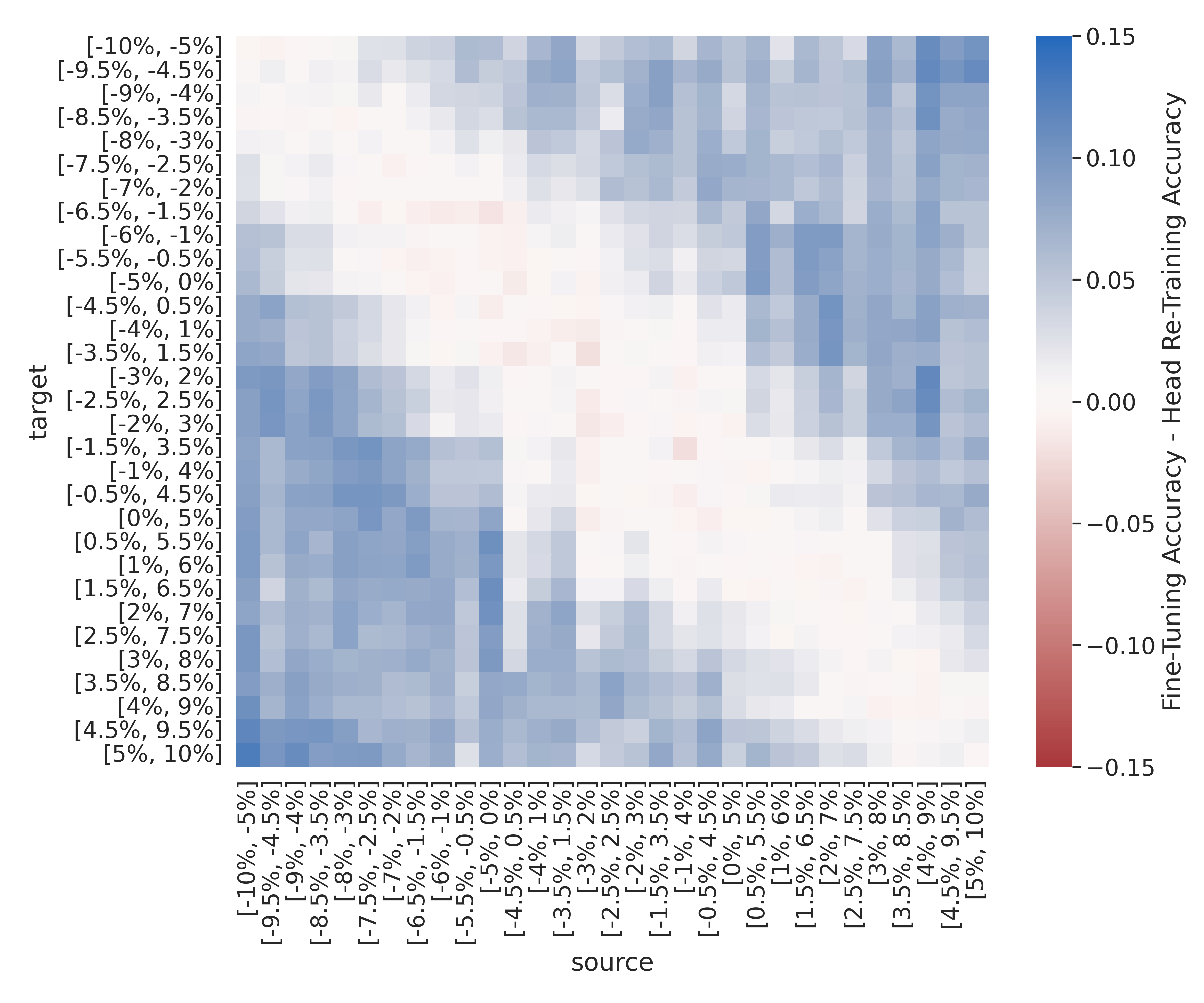
The heatmaps in Figs. 6-8 show the post-transfer top-1 accuracy achieved with each of the source/target pairs. Note that the post-transfer top-1 accuracy results shown in Figs. 6-8 are from the models that used head re-training to transfer from the source to target domains/datasets. However, the accuracy results from the models that used fine-tuning for transfer show the same trends.
Figs. 6-8 show that highest post-transfer performance is achieved along the diagonal of the heatmap, where the source and target domains are most similar. It should be noted that while the notion of domain similarity is ill-defined in general, for the purposes of this work, we are able to say that domains are more similar when the difference between the source and target signal-to-noise ratio and/or frequency offset ranges is smaller, as all other data generation parameters are held constant. These trends are expected, as models trained on similar domains likely learn similar features, and is consistent with the general theory of transfer learning Pan and Yang 2010, as well as existing works in modalities outside of radio frequency Rosenstein et al. 2005.
Figs. 6-8 also show that transfer across changes in frequency offset is approximately symmetric, while transfer across changes in signal-to-noise ratio are not. This behavior is also expected, and can be attributed to changes in the relative “difficulty” between the source and target domains. More specifically, changing the source/target signal-to-noise ratio inherently changes the difficulty of the problem, as performing automatic modulation classification in lower signal-to-noise ratio channel environments is more challenging than performing automatic modulation classification in high signal-to-noise ratio channel environments. Therefore, the source models trained on the lower signal-to-noise ratio ranges will transfer to the higher signal-to-noise ratio ranges, though may not perform optimally, while the source models trained on the higher signal-to-noise ratio ranges will fail to transfer to the lower signal-to-noise ratio ranges, as shown in Figs. 6 and 8. In contrast, changing the source/target frequency offset does not make performing automatic modulation classification any more or less difficult, but may require modifications to the learned features to accommodate which can be likened to performing frequency offset calibration, as is standard practice in radio frequency receiver operations. Consequently, small changes in frequency offset, , in either the positive and negative direction, are expected to perform similarly. Figure 7 indeed shows that transfer learning performance is approximately symmetric, with best performance closest to the diagonal where the source and target frequency offset ranges are most closesly aligned.
Practically, these trends indicate that the effectiveness of radio frequency domain adaptation increases as the source and target domains become more and more similar, and, when applicable, radio frequency domain adaptation is more often successful when transferring from harder to easier domains when compared to transferring from easier to harder domains. For example, transferring from [-5dB, 0dB] to [0dB, 5dB] signal-to-noise ratio is likely more effective than transferring from [5dB, 10dB] to [0dB, 5dB] signal-to-noise ratio because although the similarity of between datasets in these two transfer scenarios is the same, [-5dB, 0dB] is a more challenging domain than [0dB, 5dB] whereas [5dB, 10dB] is an easier domain than [0dB, 5dB]. However, transferring from a frequency offset range of [-9%, -4%] of sample rate to [-8%, -3%] of sample rate is likely more effective than transferring from a frequency offset range of [-10%, -5%] of sample rate to [-8%, -3%] of sample rate because [-9%, -4%] of sample rate and [-8%, -3%] of sample rate are more similar than [-10%, -5%] of sample rate and [-8%, -3%] of sample rate.


4.1.2 Environment Adaptation vs. Platform Adaptation
Recalling that the sweep over signal-to-noise ratio can be regarded as an environment adaptation experiment and the sweep over frequency offset can be regarded as a platform adaptation experiment, more general conclusions can be drawn regarding the challenges that environment and platform adaptation present. From the discussion in the previous subsection regarding the impact that signal-to-noise ratio and frequency offset have on the relative difficulty of the automatic modulation classification task, it follows that changes in signal-to-noise ratio are likely more challenging to overcome than changes in frequency offset. That is, changes in channel environment are more challenging to overcome using transfer learning techniques than changes in transmitter/receiver hardware, such that environment adaptation is more difficult to achieve than platform adaptation While this trend is indirectly shown through the range of accuracies achieved in Figs. 6-8, which is smaller for the frequency offset sweep than the signal-to-noise ratio sweep and signal-to-noise ratio frequency offset sweep, and is more directly shown in Figs. 9 and 10.
Figs. 9 and 10 present the difference between post-transfer top-1 accuracy and target baseline accuracy for the signal-to-noise ratio and frequency offset sweeps, such that when the difference value is positive the transfer learning model outperforms the baseline model and vice versa. These results show that for the sweep over signal-to-noise ratio, the transfer learning model only outperforms the baseline near the diagonal where the source and target are very similar. However, for the sweep over frequency offset, the transfer learning model outperforms the baseline for a greater number of source/target pairs.
From these results, we can conclude that in practice transfer learning is more useful for overcoming platform discrepancies than channel discrepancies, unless the channel discrepancy is small. If the channel discrepancy between source and target is large, one might consider simply training for random initialization on the target data to achieve top performance. Furthermore, if choosing a source dataset/model for a given target domain/task, one should consider the similarity of of the source/target channel environment before the similarity of the source/target platform, as changes in transmitter/receiver pair are more easily overcome during transfer learning.


4.1.3 Head Re-Training vs. Fine-Tuning
Figs. 11 - 13 plot the difference between post-transfer top-1 accuracies achieved using head re-training versus fine-tuning such that positive values correspond to better fine-tuning performance and negative values correspond to better head re-training performance. These figures indicate that head re-training is as effective, if not more effective, than fine-tuning when the source and target domains are similar. Meanwhile, fine-tuning is more effective when the source and target domains are more dissimilar. Intuitively, this means that when the source/target domains are dissimilar, the features found in the early layers of the source model needed modification to discern between modulation types in the target domain. However, recalling that Figs. 9 and 10 showed transfer learning only provides benefit when the source and target are somewhat similar, we can conclude that head re-training is as effective, if not more effective, than fine-tuning in the settings where transfer learning increases performance over the baseline. Given that head re-training is more time efficient and less computationally expensive than fine-tuning, there is a strong case for using head re-training over fine-tuning when performing radio frequency domain adaptation.


4.2 When and How is RF Sequential Learning Most Successful?
4.2.1 Sequential Learning Across Signal Types: Modulation Experiment 1
Fig. 14 shows the post-transfer top-1 accuracy for each source/target dataset in Modulation Experiment 1. As in the domain adaptation experiments discussed previously, the best transfer generally occurs along the diagonal of the heatmap, where the source/target similarity is highest. Additionally, the subsets containing only a single type of modulation scheme (i.e. the analog, frequency-shifted, linear subsets) don’t transfer well between one another, and also don’t transfer well to the subsets which contain multiple types of modulation schemes (i.e. the small and all subsets). Meanwhile, the small and all subsets transfer fairly well to the analog, frequency-shifted, and linear subsets. These results are verified by the results shown in Fig. 15 which presents the difference between post-transfer top-1 accuracy and the baseline target models, and shows that transfer learning only increases performance over the baseline models when there is significant overlap between the modulation schemes in each subset.
These results are expected when we consider the general setting in which transfer learning is beneficial: when the source and target are “similar”. When no similar signal types between source/target there is little-to-no benefit to using transfer learning, such as when attempting transfer between the analog, frequency-shifted, and linear subsets. However, because the small and all subsets contain at least one modulation scheme from each of the analog, frequency-shifted, and linear subsets, the pre-trained source model has some prior knowledge of each category of modulation schemes from which to build. Practically, these results indicate that transfer learning is only beneficial when similar signal types in the source and target datasets.


4.2.2 Sequential Learning For Successive Model Refinement: Modulation Experiment 2
Figs. 16 and 17 present the post-transfer top-1 accuracy and the difference between the post-transfer top-1 accuracy for Modulation Experiment 2 and target baseline accuracy for Modulation Experiment 2 respectively. These results indicate that it is easier to remove output classes during the transfer learning phase than it is to add output classes, as evidenced by higher performance in the upper triangle of the heatmap in Fig. 16, as well as the significant performance benefits over the target baseline models shown in Fig. 17. This behavior is expected, as, intuitively, it is easier to forget or disregard prior knowledge than to acquire new knowledge during transfer. More specifically, by pre-training on a larger subset of signal types (i.e. outputs), the source model has already learned features to identify all of the modulation classes in the target task. In fact, the source model has likely learned more features than necessary to perform the target task, and could undergo feature pruning in order to reduce computational complexity. It should also be noted that the task gets easier as output classes are removed, further contributing to the trend. Practically, these results dictate that one should utilize a source task that encompasses the target task, when possible.

4.2.3 Head Re-training vs. Fine Tuning
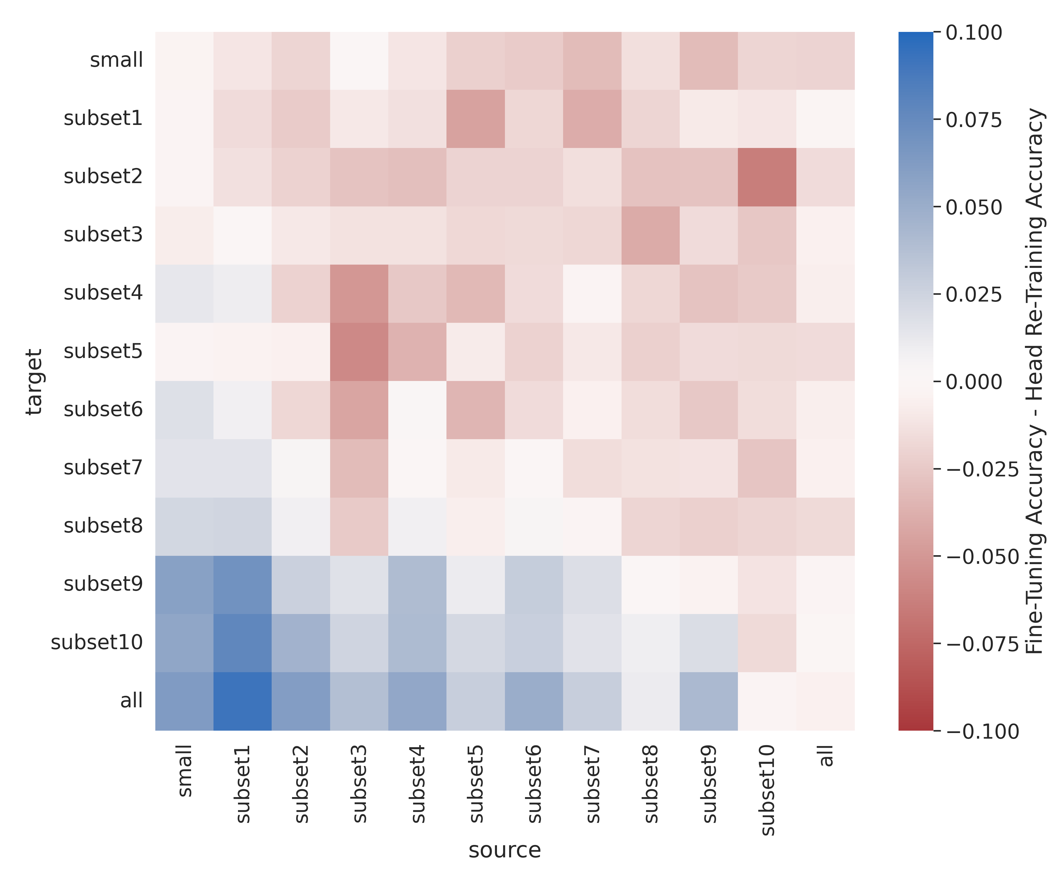
Finally, Figs. 18 and 19 present the difference between post-transfer top-1 accuracies achieved using head re-training versus fine-tuning for Modulation Experiments 1 and 2 respectively. These results show that fine-tuning outperforms head re-training in all cases where the source/target tasks are ‘less similar.” Meanwhile, when the source/target subsets have some modulation schemes in common, head re-training outperforms fine-tuning. However, as was the case in the domain adaptation experiments discussed in Section 4.1.3, head re-training is as effective, if not more effective, than fine-tuning in the settings where transfer learning increases performance over the baseline. Therefore, head re-training is the preferred method of performing radio frequency sequential learning as well, as head re-training is generally more time efficient and less computationally expensive than fine-tuning.
5 Conclusion
Transfer learning has yielded tremendous performance benefits in computer vision and natural language processing, and as a result, transfer learning is all but commonplace in these fields. However, the benefits of transfer learning have yet to be fully demonstrated and integrated in radio frequency machine learning. To begin to address this deficit, this work systematically evaluated radio frequency transfer learning performance as a function of signal-to-noise ratio, frequency offset, and modulation type for an automatic modulation classification use-case. Through this exhaustive study, a number of guidelines have been identified for when and how to use radio frequency transfer learning successfully. More specifically, results indicate:
• Using source models trained on the most similar domain/task to the target yields highest performance
• Transferring from a more challenging domain/task than the target, is preferred to transferring from an easier domain/task
• Selecting source models based on the similarity of the source/target channel environment is more important than the similarity of the source/target platform(s)
• Head re-training generally provides the highest performance in any radio frequency transfer learning case where transfer learning provides a performance benefit over training from random initialization, as measured by post-transfer top-1 accuracy, time efficiency, and computational complexity.
As previously mentioned these initial guidelines are subject to further experimentation using additional signal types, channel models, use-cases, model architectures, and augmented or captured datasets. Continuing and extending the analysis conducted herein will provide a more thorough understanding of radio frequency transfer learning behavior and performance across a wider range of use-cases and deployment settings. Further experimentation should include:
• An analysis of multi-task learning behavior using synthetic and/or captured data
• Analyses of radio frequency transfer learning performance across other metadata parameters-of-interest such as fading/multi-path channel environments, sample rate, In-phase/Quadrature imbalance, etc.
• Analyses of transfer learning performance for other radio frequency machine learning use-cases such as specific emitter identification, signal detection, etc.
• An analysis of radio frequency transfer learning techniques for transferring between use-cases. For example, can sequential learning techniques be used to transfer between automatic modulation classification and specific emitter identification use-cases? Is multi-task learning better suited to performing this type of transfer?
• Analyses of radio frequency transfer learning performance across varying domains/tasks using captured data
• An analysis of radio frequency transfer learning performance across synthetic, augmented, and captured datasets
Provided future verification and refinement of these results and guidelines, these guidelines can be used in future radio frequency machine learning systems to construct the highest performing models for a given target domain when data is limited. More specifically, these guidelines begin a discussion regarding how best to continually update radio frequency machine learning models once deployed, in an online or incremental fashion, to overcome the highly fluid nature of modern communication systems Wong et al. 2021.
Author Contributions
Conceptualization, Lauren J. Wong; methodology, Lauren J. Wong, Sean McPherson, and Alan J. Michaels; software, Lauren J. Wong; validation, Lauren J. Wong, Sean McPherson, and Alan J. Michaels; formal analysis, Lauren J. Wong; investigation, Lauren J. Wong; resources, Sean McPherson; data curation, Lauren J. Wong; writing—original draft preparation, Lauren J. Wong; writing—review and editing, Sean McPherson and Alan J. Michaels; visualization, Lauren J. Wong; supervision, Sean McPherson and Alan J. Michaels; project administration, Sean McPherson and Alan J. Michaels; funding acquisition, Not Applicable. All authors have read and agreed to the published version of the manuscript.
Funding
This research received no external funding.
Institutional Review Board Statement
Not applicable.
Informed Consent Statement
Not applicable.
Data Availability Statement
The dataset used in this work is publicly available on IEEE DataPort at https://ieee-dataport.org/open-access/transfer-learning-rf-domain-adaptation-%E2%80%93-synthetic-dataset.
Conflicts of Interest
The authors declare no conflict of interest.
Abbreviations
The following abbreviations are used in this manuscript:
- AM-DSB
amplitude modulation, double-sideband
- AM-DSBSC
amplitude modulation, double-sideband suppressed-carrier
- AM-LSB
amplitude modulation, lower-sideband
- AM-USB
amplitude modulation, upper-sideband
- AMC
automatic modulation classification
- APSK16
amplitude and phase-shift keying, order 16
- APSK32
amplitude and phase-shift keying, order 32
- AWGN
additive white Gaussian noise
- BPSK
binary phase-shift keying
- CLDNN
convolutional long-short term deep neural network
- CNN
convolutional neural network
- CV
computer vision
- DARPA
Defense Advanced Research Projects Agency
- DL
deep learning
- DNN
deep neural network
- FM-NB
narrow band frequency modulation
- FM-WB
wide band frequency modulation
- FO
frequency offset
- FSK5k
frequency-shift keying, 5kHz carrier spacing
- FSK75k
frequency-shift keying, 75kHz carrier spacing
- GFSK5k
Gaussian frequency-shift keying, 5kHz carrier spacing
- GFSK75k
Gaussian frequency-shift keying, 75kHz carrier spacing
- GMSK
Gaussian minimum-shift keying
- IQ
in-phase/quadrature
- LEEP
Log Expected Empirical Prediction
- LogME
Logarithm of Maximum Evidence
- LSTM
Long Short-Term Memory
- ML
machine learning
- MLP
multi-layer perceptrons
- MSK
minimum-shift keying
- NLP
natural language processing
- NN
neural network
- OQPSK
offset quadrature phase-shift keying
- PSK16
phase-shift keying, order 16
- PSK8
phase-shift keying, order 8
- QAM16
quadrature amplitude modulation, order 16
- QAM32
quadrature amplitude modulation, order 32
- QAM64
quadrature amplitude modulation, order 64
- QPSK
quadrature phase-shift keying
- RF
radio frequency
- RFML
radio frequency machine learning
- RNN
Recurrent Neural Network
- RRC
root-raised cosine
- SEI
specific emitter identification
- SNR
signal-to-noise ratio
- TL
transfer learning
References
- Morocho-Cayamcela et al. (2019) Morocho-Cayamcela, M.E.; Lee, H.; Lim, W. Machine Learning for 5G/B5G Mobile and Wireless Communications: Potential, Limitations, and Future Directions. IEEE Access 2019, 7, 137184–137206. https://doi.org/10.1109/ACCESS.2019.2942390.
- Wong et al. (2021) Wong, L.J.; Clark, W.H.; Flowers, B.; Buehrer, R.M.; Headley, W.C.; Michaels, A.J. An RFML Ecosystem: Considerations for the Application of Deep Learning to Spectrum Situational Awareness. IEEE Open Journal of the Communications Society 2021, 2, 2243–2264. https://doi.org/10.1109/OJCOMS.2021.3112939.
- Clark IV et al. (2021) Clark IV, W.H.; Hauser, S.; Headley, W.C.; Michaels, A.J. Training data augmentation for deep learning radio frequency systems. The Journal of Defense Modeling and Simulation 2021, 18, 217–237.
- Hauser (2018) Hauser, S.C. Real-World Considerations for Deep Learning in Spectrum Sensing. Master’s thesis, Virginia Tech, 2018.
- Sankhe et al. (2019) Sankhe, K.; Belgiovine, M.; Zhou, F.; Riyaz, S.; Ioannidis, S.; Chowdhury, K. ORACLE: Optimized Radio Classification through Convolutional Neural Networks. In Proceedings of the IEEE INFOCOM 2019-IEEE Conference on Computer Communications. IEEE, 2019, pp. 370–378.
- Ruder (2019) Ruder, S. Neural transfer learning for natural language processing. PhD thesis, NUI Galway, 2019.
- Olivas et al. (2009) Olivas, E.S.; Guerrero, J.D.M.; Martinez-Sober, M.; Magdalena-Benedito, J.R.; Serrano, L.; et al. Handbook of research on machine learning applications and trends: Algorithms, methods, and techniques; IGI Global, 2009.
- Wong and Michaels (2022) Wong, L.J.; Michaels, A.J. Transfer Learning for Radio Frequency Machine Learning: A Taxonomy and Survey. Sensors 2022, 22. https://doi.org/10.3390/s22041416.
- (9) Rondeau, T. Radio Frequency Machine Learning Systems (RFMLS).
- Dobre et al. (2007) Dobre, O.A.; Abdi, A.; Bar-Ness, Y.; Su, W. Survey of automatic modulation classification techniques: classical approaches and new trends. IET Communications 2007, 1, 137–156.
- West and O’Shea (2017) West, N.E.; O’Shea, T. Deep architectures for modulation recognition. In Proceedings of the 2017 IEEE Int. Symp. on Dynamic Spectrum Access Networks (DySPAN), 2017, pp. 1–6.
- Pan and Yang (2010) Pan, S.J.; Yang, Q. A Survey on Transfer Learning. IEEE Trans. on Knowledge and Data Eng. 2010, 22, 1345–1359. https://doi.org/10.1109/TKDE.2009.191.
- Chen et al. (2019) Chen, S.; Zheng, S.; Yang, L.; Yang, X. Deep Learning for Large-Scale Real-World ACARS and ADS-B Radio Signal Classification. IEEE Access 2019, 7, 89256–89264. https://doi.org/10.1109/ACCESS.2019.2925569.
- Pati et al. (2020) Pati, B.M.; Kaneko, M.; Taparugssanagorn, A. A Deep Convolutional Neural Network Based Transfer Learning Method for Non-Cooperative Spectrum Sensing. IEEE Access 2020, 8, 164529–164545. https://doi.org/10.1109/ACCESS.2020.3022513.
- Kuzdeba et al. (2021) Kuzdeba, S.; Robinson, J.; Carmack, J. Transfer Learning with Radio Frequency Signals. In Proceedings of the 2021 IEEE 18th Annual Consumer Communications Networking Conference (CCNC), 2021, pp. 1–9. https://doi.org/10.1109/CCNC49032.2021.9369550.
- Robinson and Kuzdeba (2021) Robinson, J.; Kuzdeba, S. RiftNet: Radio Frequency Classification for Large Populations. In Proceedings of the 2021 IEEE 18th Annual Consumer Communications Networking Conference (CCNC), 2021, pp. 1–6. https://doi.org/10.1109/CCNC49032.2021.9369455.
- O’Shea et al. (2018) O’Shea, T.J.; Roy, T.; Clancy, T.C. Over-the-Air Deep Learning Based Radio Signal Classification. IEEE Journal of Selected Topics in Signal Processing 2018, 12, 168–179. https://doi.org/10.1109/JSTSP.2018.2797022.
- Dörner et al. (2018) Dörner, S.; Cammerer, S.; Hoydis, J.; t. Brink, S. Deep Learning Based Communication Over the Air. IEEE Journal of Selected Topics in Signal Processing 2018, 12, 132–143. https://doi.org/10.1109/JSTSP.2017.2784180.
- Zheng et al. (2020) Zheng, S.; Chen, S.; Qi, P.; Zhou, H.; Yang, X. Spectrum sensing based on deep learning classification for cognitive radios. China Comm. 2020, 17, 138–148. https://doi.org/10.23919/JCC.2020.02.012.
- Clark et al. (2019) Clark, B.; Leffke, Z.; Headley, C.; Michaels, A. Cyborg Phase II Final Report. Technical report, Ted and Karyn Hume Center for National Security and Technology, 2019.
- Peng et al. (2020) Peng, Q.; Gilman, A.; Vasconcelos, N.; Cosman, P.C.; Milstein, L.B. Robust Deep Sensing Through Transfer Learning in Cognitive Radio. IEEE Wireless Comm. Letters 2020, 9, 38–41. https://doi.org/10.1109/LWC.2019.2940579.
- Ye et al. (2020) Ye, N.; Li, X.; Yu, H.; Zhao, L.; Liu, W.; Hou, X. DeepNOMA: A Unified Framework for NOMA Using Deep Multi-Task Learning. IEEE Trans. on Wireless Comm. 2020, 19, 2208–2225. https://doi.org/10.1109/TWC.2019.2963185.
- Clark et al. (2019) Clark, W.H.; Arndorfer, V.; Tamir, B.; Kim, D.; Vives, C.; Morris, H.; Wong, L.; Headley, W.C. Developing RFML Intuition: An Automatic Modulation Classification Architecture Case Study. In Proceedings of the 2019 IEEE Military Comm. Conference (MILCOM), 2019, pp. 292–298. https://doi.org/10.1109/MILCOM47813.2019.9020949.
- Wong and McPherson (2021) Wong, L.J.; McPherson, S. Explainable Neural Network-based Modulation Classification via Concept Bottleneck Models. In Proceedings of the 2021 IEEE Computing and Comm. Workshop and Conference (CCWC), 2021.
- Clark IV et al. (2021) Clark IV, W.H.; Hauser, S.; Headley, W.C.; Michaels, A.J. Training Data Augmentation for Deep Learning Radio Frequency Systems. JDMS Special Issue 2021.
- Merchant (2019) Merchant, K. Deep Neural Networks for Radio Frequency Fingerprinting. PhD thesis, 2019.
- Liu et al. (2020) Liu, Z.; Lian, T.; Farrell, J.; Wandell, B.A. Neural network generalization: The impact of camera parameters. IEEE Access 2020, 8, 10443–10454.
- (28) Gaeddert, J. liquid-dsp.
- Wong et al. (2022) Wong, L.J.; McPherson, S.; Michaels, A.J. Transfer Learning for RF Domain Adaptation – Synthetic Dataset, 2022.
- Hilburn et al. (2018) Hilburn, B.; West, N.; O’Shea, T.; Roy, T. SigMF: the signal metadata format. In Proceedings of the Proceedings of the GNU Radio Conference, 2018, Vol. 3.
- Wong and McPherson (2021) Wong, L.J.; McPherson, S. Explainable Neural Network-based Modulation Classification via Concept Bottleneck Models. In Proceedings of the 2021 IEEE 11th Annual Computing and Communication Workshop and Conference (CCWC), 2021, pp. 0191–0196. https://doi.org/10.1109/CCWC51732.2021.9376108.
- O’Shea et al. (2016) O’Shea, T.J.; Corgan, J.; Clancy, T.C. Convolutional radio modulation recognition networks. In Proceedings of the International conference on engineering applications of neural networks. Springer, 2016, pp. 213–226.
- Kingma and Ba (2014) Kingma, D.P.; Ba, J. Adam: A method for stochastic optimization. arXiv preprint arXiv:1412.6980 2014.
- (34) Cross Entropy Loss.
- Paszke et al. (2019) Paszke, A.; Gross, S.; Massa, F.; Lerer, A.; Bradbury, J.; Chanan, G.; Killeen, T.; Lin, Z.; Gimelshein, N.; Antiga, L.; et al. PyTorch: An imperative style, high-performance deep learning library. Advances in neural information processing systems 2019, 32, 8026–8037.
- Rosenstein et al. (2005) Rosenstein, M.T.; Marx, Z.; Kaelbling, L.P.; Dietterich, T.G. To transfer or not to transfer. In Proceedings of the NIPS 2005 workshop on transfer learning, 2005, Vol. 898, pp. 1–4.