Green Learning: Introduction, Examples and Outlook
Abstract
Rapid advances in artificial intelligence (AI) in the last decade have largely been built upon the wide applications of deep learning (DL). However, the high carbon footprint yielded by larger and larger DL networks becomes a concern for sustainability. Furthermore, DL decision mechanism is somewhat obscure and can only be verified by test data. Green learning (GL) has been proposed as an alternative paradigm to address these concerns. GL is characterized by low carbon footprints, small model sizes, low computational complexity, and logical transparency. It offers energy-effective solutions in cloud centers as well as mobile/edge devices. GL also provides a clear and logical decision-making process to gain people’s trust. Several statistical tools have been developed to achieve this goal in recent years. They include unsupervised representation learning, supervised feature learning, and supervised decision learning. We have seen a few successful GL examples with performance comparable with state-of-the-art DL solutions. This paper offers an introduction to GL, its demonstrated applications, and future outlook.
Keywords machine learning, green learning, trust learning, deep learning.
1 Introduction
There have been rapid advances in artificial intelligence (AI) and machine learning (ML) in the last decade. The breakthrough has largely been built upon the construction of larger datasets and the design of complex neural networks. Representative neural networks include the convolutional neural network (CNN) (Gu et al. 2018), the recurrent neural network (RNN), (Pascanu et al. 2013; Salehinejad et al. 2017; Su et al. 2022) the long short-term memory network (LSTM) (Greff et al. 2016; Hochreiter and Schmidhuber 1997; Su and Kuo 2019), etc. Deep neural networks (DNNs) have attracted a lot of attention from academia and industry since its resurgence in 2012 (Krizhevsky et al. 2012). As networks become larger and deeper, this discipline is named deep learning (DL) (LeCun et al. 2015). DL has made great impacts in various application domains, include computer vision, natural language processing, autonomous driving, robotics navigation, etc.
DL is characterized by two design choices: the network architecture and the loss function. Once these two choices are specified, model parameters can be automatically determined via an end-to-end optimization algorithm called backpropagation. When the number of training samples is less than the number of model parameters, it is common to adopt pre-trained networks to build larger networks for better performance; e.g., ResNet (He et al. 2015) or DenseNet (Huang et al. 2017) pretrained by ImageNet (Deng et al. 2009). Another emerging trend is the adoption of the transformer architecture (Han et al. 2022; Jaderberg et al. 2015; Khan et al. 2021; Vaswani et al. 2017; Wolf et al. 2020).
Despite its rapid advance, the DL paradigm faces several challenges. DL networks are mathematically intractable, vulnerable to adversarial attacks (Akhtar and Mian 2018), and demand heavy supervision. Efforts have been made in explaining the behavior of DL networks with certain success, e.g., (Chan et al. 2022; Damian et al. 2022; Ma et al. 2022; Oymak et al. 2021; Soltanolkotabi et al. 2018; Wright and Ma 2022). Adversarial training has been developed to provide a tradeoff between robustness and accuracy (Zhang et al. 2019a). Self-supervised (Misra and Maaten 2020) and semi-supervised learning (Sohn et al. 2020; Van Engelen and Hoos 2020) have been explored to reduce the supervision burden.
Two further concerns over DL technologies are less addressed. The first one is about its high carbon footprint (Lannelongue et al. 2021; Schwartz et al. 2020; Wu et al. 2022; Xu et al. 2021). The training of DL networks is computationally intensive. The training of larger complex networks on huge datasets imposes a threat on sustainability (Sanh et al. 2019; Sharir et al. 2020; Strubell et al. 2019). The second one is related to its trusworthiness. The application of blackbox DL models to high stakes decisions is questioned (Arrieta et al. 2020; Poursabzi-Sangdeh et al. 2021; Rudin 2019). Conclusions drawn from a set of input-output relationships could be misleading and counter intuition. It is essential to justify an ML prediction procedure with logical reasoning to gain people’s trust.
To tackle the first problem, one may optimize DL systems by taking performance and complexity into account jointly. An alternative solution is to build a new learning paradigm of low carbon footprint from scratch. For the latter, since it targets at green ML systems by design, it is called green learning (GL). The early development of GL was initiated by an effort to understand the operation of computational neurons of CNNs in (Kuo 2017; Kuo 2016; Kuo and Chen 2018; Kuo et al. 2019). Through a sequence of investigations, building blocks of GL have been gradually developed, and more applications have been demonstrated in recent years. As to the second problem, a clear and logical description of the decision-making process is emphasized in the development of GL. GL adopts a modularized design. Each module is statistically rooted with local optimization. GL avoids end-to-end global optimization for logical transparency and computational efficiency. On the other hand, GL exploits ensembles heavily in its learning system to boost the overall decision performance. GL yields probabilistic ML models that allow trust and risk assessment with certain performance guarantees.
GL attempts to address the following problems to make the learning process efficient and effective:
- 1.
How to remove redundancy among source image pixels for concise representations?
- 2.
How to generate more expressive representations?
- 3.
How to select discriminant/relevant features based on labels?
- 4.
How to achieve feature and decision combinations in the design of powerful classifiers/regressors?
- 5.
How to design an architecture that enables rich ensembles for performance boosting?
New and powerful tools have been developed to address each of them in the last several years, e.g., the Saak (Kuo and Chen 2018) and Saab transforms (Kuo et al. 2019) for Problem 1, the PixelHop (Chen and Kuo 2020), PixelHop++ (Chen et al. 2020a) and IPHop (Yang et al. 2022a) learning systems for Problem 2, the discriminant and relevant feature tests (Yang et al. 2022b) for Problem 3, the subspace learning machine (Fu et al. 2022a) for Problem 4. The original ideas scattered around in different papers. They will be systematically introduced here.
In this overview paper, we intend to elaborate on GL’s development, building modules and demonstrated applications. We will also provide an outlook for future R&D opportunities. The rest of this paper is organized as follows. The genesis of GL is reviewed in Sec. 2. A high-level sketch of GL is presented in Sec. 3. GL’s methodology and its building tools are detailed in Sec. 4. Illustrative application examples of GL are shown in Sec. 5. Future technological outlook is discussed in Sec. 6. Finally, concluding remarks are given in Sec. 7.
2 Genesis of Green Learning
The proven success of DL in a wide range of applications gives a clear indication of its power although it appears to be a mystery. Research on GL was initiated by providing a high-level understanding of the superior performance of DL (Kuo 2016; Kuo 2017; Xu et al. 2017). There was no attempt in giving a rigorous treatment but obtaining insights into a set of basic questions such as:
- •
What is the role of nonlinear activation (Kuo 2016)?
- •
What are individual roles played by the convolutional layers and the fully-connected (FC) layers (Kuo et al. 2019)?
- •
Is there a guideline in the network architecture design (Kuo et al. 2019)?
- •
Is it possible to avoid the expensive backpropagation optimization process in filter weight determination (Kuo and Chen 2018; Kuo et al. 2019; Lin et al. 2022)?
As the understanding increases, it becomes apparent that one can develop a new learning pipeline without nonlinear activation and backpropagation.

2.1 Anatomy of Computational Neurons
As shown in Fig. 1, a computational neuron consists of two stages in cascade: 1) an affine transformation that maps an -dimensional input vector to a scalar, and 2) a nonlinear activation operator. The affine transformation is relatively easy to understand. Yet, nonlinear activation obscures the function of a computational neuron. If the function of nonlinear activation is well understood, one may remove it and compensate its function with another mechanism. As explained in Sec. 2.2, one neural network achieves two objectives simultaneously (Kuo et al. 2019): 1) finding an expressive embedding of the input data, and 2) making decision (i.e., classification or regression) based on data embedding.
An affine transformation contains weights and bias for an input vector of dimension . According to the analysis in (Fu et al. 2022a; Lin et al. 2022), weights and biases play different roles. To determine proper weights of an affine transformation is equivalent to finding a discriminant 1D projection for partitioning. For example, one can use the linear discriminant analysis (LDA) to find a hyper-plane that partitions the whole space into two halves. The weight vector is the surface normal of the hyper-plane. In other words, the affine transformation defines a projection onto a line through the inner product of an input vector and the weight vector. Then bias term defines the split point in the projected 1D space (i.e., greater, equal and less than zero). The role of nonlinear activation was investigated for CNNs in (Kuo 2016) and multi-layer perceptrons (MLPs) in (Lin et al. 2022). It is used to avoid the sign confusion problem caused by two neurons in cascade.

2.2 Anatomy of Neural Networks
MLPs have been commonly used as a classifier. The convolutional neural networks (CNNs) can be viewed as the cascade of two sub-networks: the convolutional layers and the FC layers. One simple example called the LeNet-5 (LeCun et al. 1998) is illustrated in Fig. 2. It is convenient to have a rough breakdown of their functions as done in (Kuo et al. 2019). That is, the first sub-network is used to find powerful embeddings while the second sub-network is used for decision making. Admittedly, this anatomy is too simplistic for more complicated networks such as ResNet (He et al. 2015), DenseNet (Huang et al. 2017) and Transformers (Vaswani et al. 2017). Yet, this viewpoint is helpful in deriving the GL framework. We will elaborate on the first and the second sub-networks in Secs. 2.2.1 and 2.2.2
2.2.1 Feature Subnet
Modern DL networks have inputs, outputs, and intermediate embeddings. Their dimensions for image/video data are generally large. Consider two examples below.
Example 1. An image in the MNIST dataset has gray-scale pixels of spatial resolution . Its raw dimension is 1,024. LeNet-5 (LeCun et al. 1998) was designed for the MNIST dataset. It has two cascaded convolutional-pooling layers. At the output of the 2nd convolutional-pooling layers, one obtains an embedding space of dimension .
Example 2. After image size normalization, an image in the ImageNet dataset has color pixels of spatial resolution . It has a raw dimension of . AlexNet (Krizhevsky et al. 2012) and VGG-16 (Simonyan and Zisserman 2014) were proposed to solve the object classification problem in the ImageNet dataset. The last convolutional layers of AlexNet and VGG have an embedding space of and dimensions, respectively.
The embedding dimension of the last convolutional layer is significantly smaller than the input dimension from the above two examples. Dimension reduction is essential to the simplification of a decision pipeline. It is well known that there are spatial correlations between neighboring pixels of images, which can be exploited for dimension reduction. However, dimension reduction is only one of two main functions of the feature subnet. The feature subnet needs to find discriminant dimensions at the same time.
The dimension variation at different stages of LeNet-5 is shown in Fig. 2, where a red upward arrow denotes dimension expansion and a blue downward arrow denotes dimension reduction. Dimensions increase with convolution operations in the first two layers, and dimension decreases with the (2x2)-to-(1x1) pooling operations. The increase in the dimension of an intermediate layer is determined by the network architecture. By adding more neurons and reducing the stride number, the intermediate layer will have more dimensions. More embedding variables allow the generation of more expressive embeddings. The design of network architecture highly depends on specific applications (or datasets). The search of an optimal network architecture (Elsken et al. 2019) and the associated loss function for new problems is costly.
2.2.2 Decision Subnet
MLPs have the universal approximation capability to an arbitrary function (Cybenko 1989; Hornik et al. 1989). Without loss of generality, consider the mapping from an -dimensional input to an arbitrary 1D function. The latter can be approximated by a union of piece-wise low-order polynomials. The basic unit of a piece-wise constant (or linear) approximation is a box (or a triangular-shaped) function of finite support. The form of activation determines the shape, e.g., two step activations can be used to synthesize a box function. Users are referred to (Lin et al. 2021) for more detail. For each partitioned interval, the mean value of observed output samples (or the labels of the majority class) can be assigned in a regression problem (or a classification problem). Decision making with space partitioning is essential to all ML classifiers/regressors, e.g., the support vector machine/regression (SVM/R), decision trees, random forests, gradient boosting classifiers/regressors. Yet, no nonlinear activation is required by them but neural networks. This difference will be explained in Sec. 4.4.
2.2.3 Filter Weight Determination
One characteristics of DL systems is that filter weights can be automatically adjusted by propagating decision errors backwards (i.e., backpropagation). As long as there exist negative gradients to lower the loss function, the training loss will keep going down. Many advanced network architectures are devised to allow more paths to avoid the vanishing gradient problem. Weight adjustment has different implications in the feature subnet and the decision subnet. For the feature subnet, weights are adjusted to find the most expressive embeddings under the architecture constraint. For the decision subnet, weights are fine-tuned to find discriminant 1D projections for space partitioning. Sometimes, there may not be sufficient labeled data to train DL networks. To boost the overall performance, one may build a modularized DL system, where filter weights of some modules are pre-trained by other datasets. One example is ResNet/DenseNet pretrained by ImageNet. These pre-trained modules offer embeddings to interact with other modules of the DL system.
2.3 Interpretable Feedforward-Designed CNN
The feedforward-designed convolutional neural network (FF-CNN) (Kuo et al. 2019) plays a transitional role from DL to GL. It follows the standard CNN architecture but determines the filter weights in a feedforward one-pass manner. Filter weights in the convolutional layers of FF-CNN are determined by the Saab transform without supervision.
Although a bias term is adopted by the Saab transform to address the sign confusion problem in (Kuo et al. 2019), this term is removed in the later Saab transform implementation for the following reason. The sign confusion problem actually only exists in neural network training because of the use of backpropagation optimization. In this context, one determines both the embeddings from the previous layer and the filter weights of the current layer simultaneously based on the desired output. In contrast, the input to the current layer is already given in the feedforward design, one need to determine filter weights first based on the statistics of the current input and then compute the filter responses. As a result, there is no sign confusion problem in the FF-CNN.
Filter weights in the fully-connected (FC) layers of FF-CNN are determined by linear least-squared regression (LAG). That is, in FF-CNN training, one clusters training samples of the same class into multiple sub-clusters and create a pseudo-label for each sub-cluster. For example, there are 10 labels (i.e. 0, 1, , 9) for each image. One can have 12 sub-clusters for each digit and create 120 pseudo-labels. The first FC layer maps from 400 latent variables in the last convolution layer to 120 pseudo-labels. The determination of filter weights can be formulated as a least-squared regression problem. FF-CNN has been used in the design of a privacy preservation framework in (Hu et al. 2020; Wang et al. 2022a) and integrated with ensemble learning (Chen et al. 2019a) and semi-supervised learning (Chen et al. 2019b).
3 High-Level Sketch of GL
3.1 Overview
As mentioned in Sec. 1, GL tools have been devised to achieve the following objectives:
- 1.
Remove redundancy among source samples for concise representations.
- 2.
Generate expressive representations.
- 3.
Select discriminant/relevant features based on supervision (i.e., training labels).
- 4.
Allow feature and decision combinations in classifier/regressor design.
- 5.
Propose a system architecture that enables ensembles for performance boosting.
These techniques are summarized in Table 1.
| Learning | Need of | Linear | Examples |
| Techniques | Supervision | Operation | |
| Subspace | No | Yes | Saak Transform (Kuo and Chen 2018), |
| Approximation | Saab Transform (Kuo et al. 2019) | ||
| Expressive | Maybe | Maybe | Attention, Multi- |
| Representation Generation | Stage Transform (Chen et al. 2020a) | ||
| Ensemble-enabled | Maybe | Maybe | PixelHop (Chen and Kuo 2020) |
| Architecture | PixelHop++ (Chen et al. 2020a) | ||
| Discriminant | Yes | No | Discriminant |
| Features Selection | Feature Test (Yang et al. 2022b) | ||
| Feature Space | Yes | No | Subspace Learning |
| Partitioning | Machine (Fu et al. 2022a) |
It is worthwhile to comment on differences and relationship between GL, DL and classical ML. Traditional ML consists of two building blocks: feature design and classification. Feature design is typically based on human intuition and domain knowledge. Feature extraction and decision are integrated without a clear boundary in DL. Once the parameters of DL networks are determined by end-to-end optimization, feature design becomes a byproduct. Techniques No. 1-3 in Table 1 correspond to the feature design in GL. Techniques 1 and 2 can be automated with little human involvement. Only hyper-parameters are provided by humans, which is similar to the network architecture design in DL. Technique 3 provides a feedback from labels to the learned representations so as to zoom into the most powerful subset. Unlike traditional ML, it does not demand human intuition or domain knowledge. Finally, the last module in GL is the same as the classifier in traditional ML.
The reason to decompose the feature design module in classical ML into three individual steps in GL is for the purpose of automation. For simplicity and yet without loss of generality, we use an illustrative example to explain the four modules of GL below. Consider the ML problem of recognizing 10 handwritten digits (i.e. 0, 1, , 9) with the MNIST dataset. It has 60,000 training images and 10,000 test images. Each image has a spatial resolution of pixels, where each pixel has 256 gray scales. Typically, we treat each pixel as one dimension so that the input space has dimensions. Since there are 10 output classes, we assign 10 dimensions to the output space, denoted by , where is the probability of the test image in class . Note that this problem can be well solved by a neural network solution called LeNet-5 (LeCun et al. 1998). Although LeNet-5 is a shallow network, its architecture can be generalized to deeper networks such as AlexNet (Krizhevsky et al. 2012) and VGG-16 (Simonyan and Zisserman 2014) in a straightforward manner.
3.2 Subspace Approximation
Each pixel in an image is too weak to be a discriminant for any image content. Thus, we group a set of neighboring pixels to form a basic unit. Typical units are squared blocks of size or . There exists correlation among pixels in PixelHop units. The correlation can be reduced or removed by signal transforms. Transform kernels can be either predefined or derived from the input data. The discrete cosine transform (DCT) and the wavelet transform use predefined kernels while the Karhunen-Love transform (KLT) adopts the data-driven transform kernel. Two new data-driven transforms have been introduced to tackle Subproblem 1 in the GL setting. They are the Saab (Subspace approximation via adjusted bias) transform (Kuo et al. 2019) and the Saak (Subspace approximation via augmented kernels) transform (Kuo and Chen 2018). These new transforms will be reviewed in Sec. 4.2. No supervision is needed in learning the approximating subspace.
3.3 Generation of Expressive Representations
There are many ways to conduct the 2D transform for images in the MNIST dataset. We compare the following two designs.
- A
One-stage transform.
The transform has a kernel of size . The transform input and output have the same dimension; namely, 1024. Since the element-wise energy is not uniformly distributed for the 1024D output, we drop those elements of extremely low energy to form a representation vector. - B
Two-stage transform.
The first-stage transform has a kernel size of . It is applied to interior pixels with stride equal to one. Then, we take the absolute value of each response and conduct the maximum pooling over non-overlapping blocks. This leads to a tensor output of dimension , where indicate the number of spatial locations and is the channel response of the first-stage transform. Finally, we conduct the second-stage transform to locations for each channel. The output of the second-stage transform still have a dimension of . Again, we can drop those elements of extremely low energy to form a representation vector.
Computationally, the one-stage transform is less efficient than the two-stage transform due to its large kernel size. Here, we pay attention to another issue - the expressiveness of derived representations. For fair comparison, we select the same element number (e.g., 512) of the highest energy from designs A and B as the representation vector. We may ask which representation set is more useful in the classification problem. For design A, only a few low-frequency transform coefficients are helpful since a vast majority of high-frequency transform coefficients are not stable for images of the same label. For design B, the first-stage transform captures the local variation while the second-stage transform characterizes the global variation. It has more useful representations since we can obtain more stable associations between transform coefficients and the image class. We use expressiveness to differentiate these two representation sets.
In this example, no supervision is used to derive expressive representations. However, it is sometimes useful to exploit image labels to derive the expressive representation set. One example is attention detection. Consider the classification of dog and cat images. Both dog and cat images have background, which is irrelevant to the classification task. It is desired to remove the background effect and focus on the main object, which is called the attention. To obtain attention, we can decompose images into smaller blocks, extract block-level representations and use image labels to train the probability of a block to be a dog or a cat. For the foreground object, a test cat (or dog) block is expected to have a higher probability for the cat (or dog) decision. For a background block, if has the same likelihood to be with cat and dog images, its test probability will be about equal (i.e., 50it has a higher likelihood to be with cat (or dog) images, then its test probability will be higher for the cat (or dog) class. As a result, we can use blocks with more skewed probability distribution as attention. Clearly, attention offers expressive representations that have to be trained by image labels.
Subspace approximation is used to reduce redundancy in representation. However, it is still desired to find more expressive representations that are valuable in solving the target learning problem. The former is straightforward while the latter is not. This makes GL challenging yet interesting. Since they are closely related to each other in finding an effective representation of a data source, we treat them as a whole. Details are presented in Sec. 4.2.
3.4 Ensemble-Enabled Architectures
Filter responses of DL architectures are latent variables. Their values keep evolving during the end-to-end optimization process since the filter weights are adjusted through backpropagation. The exact values of these individual latent variables are not important since they are affected by many factors such as filter weight initialization and the detailed implementation of the stochastic gradient descent optimization (e.g., the order of mini-batches and dropout). People are mainly concerned with the converged neural networks as a whole.
In contrast, filter weights in GL are determined in a feedforward one-pass manner. Once computed, they stay the same and do not change any longer. The same GL architecture will have the same filter weights and responses. GL needs other mechanisms to boost the learning performance. One idea is the "ensemble-enabled architectures" as demonstrated in PixelHop, PixelHop++, PointHop and PointHop++. Filter responses at various stages define joint spatial-spectral representations in form of 3D tensors. The 3D tensors in earlier (or later) stages have higher (or lower) spatial dimensions and smaller (or higher) spectral dimensions. They have different physical meanings. GL can conduct feature ensembles and/or decision ensembles to achieve better performance.
3.5 Discriminant Features Selection
Feature selection methods can be categorized into unsupervised (Solorio-Fernández et al. 2020), semi-supervised (Sheikhpour et al. 2017), and supervised (Huang 2015) three types. Unsupervised methods focus on the statistics of each feature dimension while ignoring the target class or value. However, their power is limited and less effective than supervised methods. Recently, Yang et al. (Yang et al. 2022b) proposed a supervised learning tool in selecting discriminant features and call it the discriminant feature test (DFT). DFT can rank the discriminant power of each dimension from the highest to the lowest and determine a threshold that separates discriminant dimensions automatically. It offers an immensely powerful tool for discriminant feature selection and will be reviewed in Sec. 4.3.
3.6 Feature Space Partitioning
After discriminant feature selection, the last step is classification that maps a sample in the feature space to a label. There are two main ideas to implement the classification task:
- A
Change of variables from input features to output label-probability vector. Examples include the logistic regression classifier (Dreiseitl and Ohno-Machado 2002), the linear least-squares regression (LLSR) classifier (Loh 2011), and the multilayer perceptron (MLP) (Rosenblatt 1958).
- B
Partitioning of the input feature space into purer cells whose samples are mostly from the same class. There are two major families: 1) the support vector machine (SVM) (Cortes and Vapnik 1995) and 2) the decision tree (DT) (Breiman et al. 1984), and its variants such as random forests (Breiman 2001) and XGBoost (Chen and Guestrin 2016; Chen et al. 2015).
Recently, Lin et al. (Lin et al. 2022) provides a geometrical interpretation to MLP that builds a bridge between the above two idea. Furthermore, Fu et al. (Fu et al. 2022a) proposed an enhanced version of DT known as the subspace learning machine (SLM) tree as well as SLM Forest and SLM Boost. They will be described in Sec. 4.4.
4 GL Methodologies
4.1 Overview of GL Systems
The architecture of a GL system departs from that of neural networks completely. A GL system does not have the computational neuron as its basic unit. Its global architecture is not a network, either. As illustrated in Fig. 3, a generic GL system consists of three learning modules in cascade: 1) unsupervised representation learning, 2) supervised feature learning and 3) supervised decision learning. The input and the output of the system are data sources and decisions, respectively. The two intermediate results are representations and features. They are not latent but explicit and observable. The entire system is characterized by three traits: feedforward design, individually optimized module, and statistical ensembles.
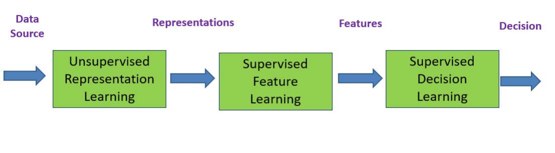
A concrete example of the GL system, called PixelHop (Chen and Kuo 2020), is shown in Fig. 4. Its three modules are elaborated below.
- •
Module #1: Derive a rich set of representations from image sources through a sequence of PixelHop units in cascade.
The main purpose of this module is to derive attributes from near-to-far pixel neighborhoods of source images without supervision (i.e. labels). Each PixelHop unit takes the neighborhood of any pixel as the input and learns its spectral representation. The Saab transform is used for dimension reduction. Furthermore, one can use spatial pooling to reduce the dimension of the whole image. The pooling process helps enlarge the neighboring size in the following PixelHop unit. - •
Module #2: Select useful features from a large set of representations.
Each PixelHop unit yields new spatial-spectral representations of the input. Their dimensions are still high. The main purpose of this module is to find a smaller set of discriminant features from a larger set of representations based on the label information for the desired task. The Label-Assisted reGressor (LAG) unit was proposed in PixelHop to achieve this objective. A more powerful tool was recently developed to replace the LAG unit in (Yang et al. 2022b), which will be discussed in Sec. 4.3. - •
Module #3: Conduct feature ensembles and the final classification task.
All features across multiple PixelHop units are concatenated to form an ensemble feature set. Then, they are fed into an ML classifier for the final classification task.

4.2 Unsupervised Representation Learning
4.2.1 Single-Stage Data-Driven Transforms
Signal transforms are widely used in signal processing to reveal spectral properties of underlying signals. Many signal transforms are data independent such as the Fourier transform, the discrete Cosine transform (DCT), and the wavelet transform. However, there are transforms that are data-driven. One famous example is KLT, which is also known as the principal component analysis (PCA). KLT can decorrelate the correlations among elements of an input signal vector and generate a compact description. In the context of computer vision, the eigenface for face recognition (Turk and Pentland 1991) was developed based on the 2D KLT.
Saak and Saab transforms were proposed to define filter weights of a computational neuron in convolutional layers of CNNs. Let us use the neuron in Fig. 1 as an example. The dimension of its input vector is . Its KLT kernel is in form of , . However, we may choose a smaller kernel number for lossy approximation. Typically, eigenvalue is ordered in a decreasing order of . If , this leads to the lossless Saab transform. If the kernel number is reduced from to , this leads to the lossy Saab transform. The Saak transform demands that filter weights appear in pairs; namely, both and co-exist so that it demands neurons. It is desired to reduce the neuron number from back to .
Also, input has to be a mean-removed vector in PCA. Although one can remove the mean of the input in the training, there is no guarantee that the training and testing data have the same mean values. To address the mean mismatch problem, the Saab transform introduce a DC kernel whose elements have the same value. The operation of the DC kernel on the input yields a local patch mean. For images that satisfy the ergodic property, the local mean can provide a good approximation to the ensemble mean. Then, one can remove the local-mean of the input and conduct PCA to generate AC kernels. For the example in Fig. 1, one DC kernel and AC kernels serve as the filter weights of neurons. To remove the effect of nonlinear activation, all filters at the same layer add the same bias such that all filter responses are positive. This filter weight design methodology is computationally efficient. Besides, it allows a simple interpretation of the role of convolutional layers.
4.2.2 Multi-Stage Transforms in Cascade
There exist long-, mid-, and short-distance correlations in images. Such correlations are handled by multiple convolutional layers in cascade in CNNs. To enlarge the receptive field of a deeper layer in CNNs, there are two choices: 1) adopting a larger stride number, and 2) applying the max-pooling operation at the output of each neuron. The same idea is followed by Module #1 in the PixelHop system.

Saab coefficients are weakly correlated in the spectral domain due to the use of PCA in their derivation. As show in Fig. 5, the weak spectral correlation enables the decomposition of a 3D (i.e., 2D spatial and 1D spectral) input tensor of dimension into spatial tensors of neighborhood size (i.e., one for each spectral component) for the th PixelHop unit, respectively. Then, instead of performing the Standard 3D Saab transform as given in the top subfigure, one applies channel-wise (c/w) Saab transforms to each of the spatial tensors as shown in the bottom subfigure. There are two advantages for c/w Saab transform. First, for the lossless Saab transform, the model size of the c/w Saab transform is smaller than that of the standard 3D Saab transform. Second, for the lossy Saab transform, the model size saving of the c/w Saab transform can be even more substantial.
To check the first point, let and denote the dimensions of the inputs to the standard and c/w Saab transforms. Then, their model sizes are:
| Standard Saab: | (1) | ||||
| C/W Saab: | (2) |
To see the second point, we show the multi-stage lossy c/w Saab transform for the whole image of size as an example in Fig. 6. For high frequency components, the spatial correlation of pixels in a local patch is so weak that its covariance matrix is a nearly diagonal matrix, and there is no need to conduct the Saab transform afterwards. These channels are colored in pink and called leaf nodes. On the other hand, for low frequency components, the spatial correlation of pixels in a local patch is still strong so that the c/w Saab transform is conducted. They are colored in gray and called intermediate nodes.

4.2.3 Enrichment of Expressive Representations

There are more ways to generate expressive representations. Two ideas were proposed in IPHOP (Yang et al. 2022a). IPHop is an improved PixelHop system. Its system diagram is shown in Fig. 7, which has two hops.
The first module of IPHop is similar to that of PixelHop++ except that max-pooling in PixelHop++ is changed to absolute-max-pooling. That is, the responses from the previous stage can be either positive or negative (without adding the bias term). Instead of clipping negative values to zero as done in the ReLU unit, we take the absolute value of all responses followed by the maximum pooling operation. The absolute-max-pooling operation gives a small gain over the straightforward max-pooling since the former preserves the low frequency components of the spatial responses at the output of any single Saab filter.
The filter responses extracted at Hop-1 and Hop-2 only have a local view on a larger object due to the limited receptive field size. Thus, they are not discriminant enough. For a given Saab filter, its responses are spatially correlated. To decorrelate them, one can conduct another Saab transform across them at each channel. This operation provides channel-wise spectral Saab representations at Hop-1 and Hop-2 as shown in the right subfigure of Fig. 7. As compared to representations learned by enlarging the neighborhood range gradually, the channel-wise spectral Saab representations can capture the long range correlation at a fine scale. The spatial and spectral Saab representations are concatenated at Hop-1 and Hop-2 to form joint-spatial-spectral Saab representations.
4.3 Supervised Feature Learning
The leverage of labels (i.e., supervision) effectively to boost the performance of a learning system is a key question in ML. Classical ML only exploits labels in the classifier design. DL uses labels to adjust filter weights in the feature subnet and the decision subnet and achieves better performance. The linear least-squared regression adopted by FF-CNN is also an example of supervised feature learning. We discuss an effective supervised learning tool in this subsection.
Existing semi-supervised and supervised feature selection methods can be classified into wrapper, filter and embedded three classes (Sheikhpour et al. 2017). Wrapper methods (Kohavi and John 1997) create multiple models with different subsets of input features and select the model containing the features that yield the best performance. One example is recursive feature elimination (RFE) (Guyon et al. 2002). This process can be computationally expensive. Filter methods involve evaluating the relationship between input and target variables using statistics and selecting those variables that have the strongest relation with the target ones. One example is the analysis of variance (ANOVA) (Scheffe 1999). This approach is computationally efficient with robust performance. Embedded methods perform feature selection in the process of training and are usually specific to a single learner. One example is “feature importance" (FI) obtained from the training process of the XGBoost classifier/regressor (Chen and Guestrin 2016; Chen et al. 2015), which is also known as “feature selection from model" (SFM). Recently, the discriminant feature test (DFT) and the relevant feature test (RFT) were proposed in (Yang et al. 2022b) for the classification and the regression problems, respectively. They belong to the filter class.

Consider a classification problem with data samples, features and classes. Let , , be a feature dimension and its minimum and maximum are and , respectively. DFT is used to measure the discriminant power of each feature dimension out of a -dimensional feature space independently. If feature is a discriminant one, one expects that data samples projected to it should be classified more easily. To check it, an idea is to partition into non-overlapping subintervals and adopt the maximum likelihood rule to assign the class label to samples inside each sub-interval. Then, one can compute the percentage of correct predictions. The higher the prediction accuracy, the higher the discriminant power. Although prediction accuracy may serve as an indicator for purity, it does not tell the distribution of the remaining classes if . Since the weighted entropy measure provides more valuable information, it was adopted in (Yang et al. 2022b).
By following the practice of a binary decision tree, the work in (Yang et al. 2022b) chose as shown in the left subfigure of Fig. 8, where denotes the threshold position of two sub-intervals. For a sample with its th dimension, , it goes to the subset associated with the left subinterval. Otherwise, it will go to the subset associated with the right subinterval. DFT and RFT uses the weight entropy and the weighted mean-squared-error (MSE) as the cost functions, respectively. The optimal cost values are computed for each feature dimension. A representation is more discriminant (or relevant) if its optimal cost value is lower. To select a set of discriminant features, one can sort representations based on their optimal cost values from the lowest to the highest and plot the curve accordingly. A representative DFT curve is shown in Fig. 9. An elbow point can be identified in most applications. Both early and late elbow points were considered in (Yang et al. 2022b). A late elbow point was illustrated in Fig. 9. The set of representations with optimal cost values lower than the elbow point are selected as features. They are enclosed by a red box in Fig. 9.

4.4 Supervised Decision Learning
Consider a classification problem with -dimensional feature vector, denoted by , and -dimensional decision vector, denoted by . The latter means that there are classes and , , is the probability of choosing class . To optimize the performance of a classifier, it is often to consider two types of manipulation:
- •
Feature Combination:
(3) where is an -dimensional weight vector.
- •
Decision Combination:
(4) where are decision vectors.
The decision learning problem is to find optimal feature weight vector and/or decision weight vector to optimize the classification performance. Table 2 lists several representative classifiers. They are categorized based on whether a feature processing operation (along columns) or a decision processing operation (along rows) is exploited in the classification procedure.
| Decision Combination | Feature Combination | ||
|---|---|---|---|
| None | One-Stage | Multi-Stage | |
| None | Decision Tree | SVM | MLP, SLM Tree |
| Ensemble | Random Forest | SLM Forest | |
| Boosting | XG Boost | SLM Boost | |
4.4.1 Classifiers Built Upon Feature Combinations
The use of feature combinations to optimize classification performance is examined in this section. Only SVM, SLM and MLP in Table 2 exploit feature combinations.
To introduce the SVM classifier, one can re-write Eq. (3) and set it to zero:
| (5) |
where is a bias. There is a physical meaning associated with Eq. (3). It corresponds to an -dimensional hyper-plane that partitions the space into two nonoverlapping half-spaces:
| (6) | |||||
| (7) |
For a simple binary classification problem, SVM chooses parameters and to maximize the separation, or margin, between the two classes. Such a hyper-plane is called the maximum-margin hyper-plane. The location of the hyper-plane is determined by a couple of specific data points called support vectors. Generally, a set of hyper-planes is determined to partition the feature space.
SVM and a single SLM tree belong to the same category in Table 2. They use different criteria to search for the optimal parameters. The optimization of an SLM tree consists of two steps. The first step is to find the most discriminant 1D direction, denoted by , that minimizes the weighted entropy of a decision under an optimal split point (or ). The second step is to project -dimensional feature vectors onto 1D feature vectors and then find the optimal split (bias) in the 1D space. A probabilistic search and an adaptive particle swarm optimization algorithm were proposed in (Fu et al. 2022a) and (Fu et al. 2022b) to implement the SLM, respectively. Actually, the stochastic gradient descent (SGD) algorithm can also be used to speed up the search of optimal combination parameters.
It is important to emphasize that the feature combination operations in SVM and SLM only yield partition hyper-planes. They do not change the feature vectors of input samples. One can evaluate the sign of to decide the location of a sample against a specific partitioned hyper-plane. When there are multiple partitioning planes, the information can be binary coded against each of the planes as explained in (Lin et al. 2022). Two samples belong to the same region if they share the same binary code. However, this is not the case in MLP.
The feature combination in Eq. (3) transforms the embeddings of all samples from their original space into a new scalar variable, denoted by , at a single neuron. If there are neurons, the embeddings of all samples evolve in the following manner:
| (8) |
where
| (9) |
The embedding combination occurs at least at two layers (e.g., one hidden layer and the output layer). A nonlinear activation unit is needed after each embedding combination step to resolve the sign confusion (Kuo 2016; Lin et al. 2022).
4.4.2 Classifiers Built Upon Decision Processing
For traditional DTs, RF is the most popular bagging ensemble algorithm. It consists of a set of tree predictors, where each tree is built based on the values of a random vector sampled independently and with the same distribution for all trees in the forest. With the Strong Law of Large Numbers, the performance of RF converges as the tree number increases. As compared to the individual DTs, significant performance improvement is achieved with the combination of many weak decision trees.
Motivated by RF, SLM Forest is developed by learning a series of single SLM tree models to enhance the predictive performance of each individual SLM tree. SLM is a predictive model stronger than DT. Besides, the probabilistic projection provides diversity between different SLM models. Following RF, SLM Forest takes the majority vote of the individual SLM trees as the ensemble result for classification tasks, and it adopts the mean of each SLM tree prediction as the ensemble result for regression tasks.
With standard DTs as weak learners, GBDT (Friedman 2001) and XGBoost (Chen et al. 2015; Chen and Guestrin 2016) can deal with a large amount of data efficiently and achieve the state-of-the-art performance in many machine learning problems. They take the ensemble of standard DTs with boosting, i.e. by defining an objective function and optimizing it with learning a sequence of DTs. By following the gradient boosting process, SLM Boost was proposed to ensemble a sequence of SLM trees in (Fu et al. 2022a). All the above discussion can be extended to the design of the subspace learning regressor (SLR).
4.5 Historical Notes
| Year | Technology | Description | Ref. |
|---|---|---|---|
| 2016 | Sign Confusion | Identified the sign confusion problem and explained | (Kuo 2016) |
| Resolution | the use of nonlinear activation to resolve it in CNNs | ||
| 2017 | RECOS | Attempted to give a physical meaning to filter weights | (Kuo 2017) |
| Transform | in CNNs | ||
| 2018 | Saak | Determined filter weights in CNNs with Saak transform | (Kuo and Chen 2018) |
| Transform | which is a variant of principal component analysis | ||
| 2019 | Saab | Determined filter weights in CNNs with Saab transform | (Kuo et al. 2019) |
| Transform | which is another variant of principal component analysis | ||
| 2019 | Label-Assisted | Attempted to link unsupervised representations with labels | (Kuo et al. 2019) |
| Regression | |||
| 2020 | PixelHop | Proposed Successive Subspace Learning (SSL), | (Chen and Kuo 2020) |
| which deviates from CNN architecture completely | |||
| 2020 | PointHop | Applied Saab transform to octant representations | (Zhang et al. 2020a) |
| targeting at point cloud data | |||
| 2020 | Channel-Wise | Proposed an effective multi-stage Saab transform | (Chen et al. 2020a; Zhang et al. 2020b) |
| Saab Trans. | applicable to PixelHop and PointHop | ||
| 2022 | DFT/RFT | Proposed effective supervised feature selection methods: | (Yang et al. 2022b) |
| Discriminant/Relevant Feature Tests | |||
| 2022 | SLM/SLR | Proposed a new classifier/regressor that allows | (Fu et al. 2022b; Fu et al. 2022a) |
| both feature and decision combinations | |||
| 2022 | IPHop | Proposed an improved PixelHop system that has new | (Yang et al. 2022a) |
| unsupervised features and replaces LAG with DFT |
- 1.
Early Exploration (2015-2017)
In the early exploration stage, the efforts focused on the understanding of the roles played by the filter weights and the nonlinear activation unit in a computational neuron of CNNs. The main objective was to shed light on the superior performance from the signal processing viewpoint since it was difficult to get engineering insights from the end-to-end non-convex optimization problem formulation. The necessity of nonlinear activation was explained in (Kuo 2016) as a mechanism to resolve the sign confusion problem in neural network training. The filter weights were explained as the memory of an CNN learning system (Kuo 2017) and used to capture local, mid-level and global intrinsic representations of objects (Xu et al. 2017). Although the explanation of the role of filter weights was preliminary, it did inspire the later work on unsupervised representation learning. - 2.
FF-CNN, Saab Transforms and channel-wise Saab Transforms (2018-2019)
Based on the foundation laid by (Kuo 2017; Xu et al. 2017), novel ways to determine filter weights of the convolutional layers in CNNs in a feedforward manner were proposed in (Kuo et al. 2019). The design is called the feedforward CNN (FF-CNN). The filter weights in convolutional layers of FF-CNN are determined by the Saab (or Saak) transforms. The transform operations are unsupervised since no class labels are used. The filter weights in FC layers of FF-CNN are determined by the label-guided least-squared regression (LAG). The main objective was to lower the training complexity with an interpretable design. - 3.
PixelHop, PixelHop++, PointHop, PointHop++, and GL Applications (2020-2021)
PixelHop (Chen and Kuo 2020) and PixelHop++ (Chen et al. 2020a) were two first-generation GL systems. They designs depart from the neural networks completely. Instead of demanding end-to-end connectivity of neurons, GL systems adopt feedforward and ensemble learning principle. Both PixelHop and PixelHop++ have three modules. They use multi-stage Saab transforms and pooling operation to yield joint spatial-spectral representations with no supervision in the first module. The LAG operation is exploited to reduce the representation dimension before being fed into classifiers in the second stage. A traditional ML classifier is used in the third stage. The main difference between PixelHop and PixelHop++ lies in the multi-stage “standard" and “channel-wise" Saab transforms. While PixelHop and PixelHop++ target at the image classification application, PointHop (Zhang et al. 2020a) and PointHop++ (Zhang et al. 2020b) were developed for the point cloud classification. Due to the irregular spatial structure of a 3D point cloud scan, a novel octant representation was introduced before the Saab transform in PointHop.We have witnessed many successful applications of GL since 2020. Their performance is comparable with that of state-of-the-art DL solutions with significantly less resource. Examples include image classification (Yang et al. 2021), image enhancement (Azizi et al. 2020), image quality assessment (Mei et al. 2022; Zhang et al. 2020c), deepfake image/video detection (Chen et al. 2022; Chen et al. 2021a; Chen et al. 2021b; Zhu et al. 2022a), point cloud classification, segmentation, registration (Kadam et al. 2021; Kadam et al. 2020; Kadam et al. 2022a; Liu et al. 2021a; Zhang et al. 2021; Zhang et al. 2020d), face biometrics (Rouhsedaghat et al. 2021a; Rouhsedaghat et al. 2021b), texture analysis and synthesis (Lei et al. 2020; Lei et al. 2021; Zhang et al. 2019b), graph node classification (Xie et al. 2022a; Xie et al. 2022b), data compression (Chen et al. 2020b; Zhang et al. 2020e), joint image compression and classification (Tseng et al. 2020), 3D medical image analysis (Ding et al. 2020; Liu et al. 2021b), etc. We will present several successful examples to provide insights for future development of GL in Sec. 5.
- 4.
Advanced GL Tools and Broader Applications (2022- )
Two advanced GL tools were developed in 2022: 1) DFT/RFT for supervised discriminant/relevant feature selection (Yang et al. 2022b) (see Sec. 4.3) and 2) SLM/SLR as a new classifier/regressor that exploits both feature combinations and decision combinations (see Sec. 4.4).Furthermore, a more advanced GL system called IPHop was proposed in (Yang et al. 2022a). It replaces the traditional max-pooling operation with the absolute-max-pooling operation and yields more unsupervised representations by introducing the spatial Saab transform at each channel in the first module of PixelHop. Furthermore, it replaces the LAG operation with DFT in the second module of PixelHop.
5 Demonstrated Examples
GL has been successfully applied to quite a few application problems. In this section, we choose five representative examples to illustrate the power of GL.
5.1 Deepfake Detection
| 2nd Generation | ||||
| Methods | Model | Celeb-DF v1 | Celeb-DF v2 | Param No. |
| Two-stream (Zhou et al. 2017a) | InceptionV3a | 55.7% | 53.8% | 23.9M |
| Meso4 (Afchar et al. 2018) | Designed CNNa | 53.6% | 54.8% | 28.0K |
| MesoInception4 (Afchar et al. 2018) | Designed CNNa | 49.6% | 53.6% | 28.6K |
| HeadPose (Yang et al. 2019a) | SVMb | 54.8% | 54.6% | - |
| FWA (Li and Lyu 2018) | ResNet-50a | 53.8% | 56.9% | 25.6M |
| VA-MLP (Matern et al. 2019) | Designed CNNa | 48.8% | 55.0% | - |
| VA-LogReg (Matern et al. 2019) | Logistic Regressionb | 46.9% | 55.1% | - |
| Xception-raw (Rossler et al. 2019) | XceptionNeta | 38.7% | 48.2% | 22.9M |
| Xception-c23 (Rossler et al. 2019) | XceptionNeta | - | 65.3% | 22.9M |
| Xception-c40 (Rossler et al. 2019) | XceptionNeta | - | 65.5% | 22.9M |
| Multi-task (Nguyen et al. 2019a) | Designed CNNa | 36.5% | 54.3% | - |
| Capsule (Nguyen et al. 2019b) | CapsuleNeta | - | 57.5% | 3.9M |
| DSP-FWA (Li and Lyu 2019) | SPPNeta | - | 64.6% | - |
| Multi-attentional (Zhao et al. 2021) | Efficient-B4a | - | 67.4% | 19.5M |
| DefakeHop++ (Chen et al. 2022) (Frame) | DefakeHop++b | 56.30% | 60.5% | 238K |
| DefakeHop++ (Chen et al. 2022) (Video) | DefakeHop++b | 58.15% | 62.4% | 238K |
| DefakeHop (Chen et al. 2021a) (Trained on Celeb-DF, Frame) | DefakeHopb | 93.1% | 87.7% | 42.8K |
| DefakeHop (Chen et al. 2021a) (Trained on Celeb-DF, Video) | DefakeHopb | 95.0% | 90.6% | 42.8K |
| DefakeHop++ (Chen et al. 2022) (Trained on Celeb-DF, Frame) | DefakeHop++b | 95.4% | 94.3% | 238K |
| DefakeHop++ (Chen et al. 2022) (Trained on Celeb-DF, Video) | DefakeHop++b | 97.5% | 96.7% | 238K |
The fast-growing Generative Adversarial Network (GAN) technology has been applied to image forgery in recent years. They are effective in reducing manipulation traces detectable by human eyes. It is challenging for humans to distinguish Deepfake images from real ones against advanced deepfake methods.
There are three generations of deepfake video datasets, which shows the evolution of deepfake techniques. The UADFV dataset (Li and Lyu 2018) belongs to the first-generation. It has 50 video clips generated by one deepfake method. Its real and fake videos can be easily detected by human eyes. FaceForensics++ (FF++) (Rossler et al. 2019), Celeb-DF-v1 and Celeb-DF-v2 (Li et al. 2020) belong to the second generation. They have more video clips with more subjects. It is difficult for humans to distinguish real and fake faces. DFDC (Dolhansky et al. 2020) is an example of the third-generation dataset. It contains more than 100K fake videos generated by 8 deepfake techniques and perturbed by 19 distortions types.
State-of-the-art deepfake detectors are based on DNNs. Although they offer high detection performance, their model sizes are exceptionally large so that they cannot be deployed on mobile phones. For example, the winning team of the DFDC contest (Seferbekov 2020) used seven pre-trained EfficientNets that contain 432 million parameters. In contrast, two lightweight deepfake detectors called DefakeHop (Chen et al. 2021a) and DefakeHop++ (Chen et al. 2022) were developed based on the GL principle. Their model sizes are significantly smaller as shown in the last column of Table 4.
The detection performance of several deepfake detectors on the second-generation datasets under cross-domain training was compared in Table 4, where AUC is used as the performance metric. For the cross-domain setting, deepfake detectors were trained on FF++ and tested on Celeb-DF-v1 and Celeb-DF-v2. As shown in the table, video-level DefakeHop++ gives the best AUC score while frame-level DefakeHop++ gives the second best for Celeb-DF-v1. As to Celeb-DF-v2, Multi-attentional yield the best AUC score while Xception-raw and Xception-c23 offer the second best scores. DefakeHop++ is slightly inferior to them. Furthermore, the performance of DefakeHop and DefakeHop++ under the same domain training is shown in the last four rows of Table 4. Their performance has improved significantly. Video-level DefakeHop++ outperforms video-level DefakeHop by 2.5% in Celeb-DF v1 and 6.1% in Celeb-DF v2.
Fig. 10 compares the detection AUC performance of MobileNet v3 and DefakeHop++ on the third-generation dataset, DFDC. MobileNet v3 is a lightweight CNN model of 1.5M parameters targeting at mobile applications, DefakeHop++ has an even smaller model size of 238K parameters (i.e., 16% of MibileNet v3). We see from Fig. 10 that DefakeHop++ outperforms MobileNet v3 without data augmentation and leverage of pre-trained models. DefakeHop++ and pretrained MobileNet v3 have similar detection performance under weak supervision.

5.2 Blind Image/Video Quality Assessment
Image/video quality assessment (QA) aims at evaluating image/video quality to facilitate image streaming. Based on the availability of undistorted reference images/videos, objective QA can be classified into three categories (Lin and Kuo 2011): full-reference (FR), reduced-referenced (RR) and no-reference (NR). The last one is also known as blind QA (BQA). FR-QA metrics have achieved high consistency with human subjective evaluation. Many FR-QA methods have been well developed in the last two decades such as SSIM (Wang et al. 2004), FSIM (Zhang et al. 2011) and VMAF (Li et al. 2018a). RR-QA metrics only utilize features of reference images/videos for quality evaluation. In some application scenarios (e.g., image receivers), users cannot access reference images/videos so that NR-QA is the only choice. BQA methods attract growing attention in recent years.
The GL technology has been applied to BIQA (blind image quality assessment) as summarized in this subsection. Conventional BIQA methods has two steps: 1) extraction of quality-aware features and 2) adoption of a regression model for quality score prediction. Recently, as the amount of user generated images grows rapidly, DNN-based BIQA methods have been proposed with significant performance improvement (Yang et al. 2019b). DNN-based solutions often rely on a huge pre-trained network which is trained by a large dataset. The large model size demands high computational complexity and memory requirement. In (Mei et al. 2022), a lightweight BIQA method, called GreenBIQA, was proposed to achieve high performance that is competitive with DNN-based solutions yet demands much less computing power and memory. To this end, for a video source, GreenBIQA can predict perceptual quality scores frame by frame in real time.
The performance of GreenBIQA is evaluated on four IQA datasets. CSIQ (Larson and Chandler 2010) and KADID-10K (Lin et al. 2019) are two synthetic-distortion datasets. They were created by applying multiple distortions of various levels to a set of reference images. LIVE-C (Ghadiyaram and Bovik 2015) and KonIQ-10K (Hosu et al. 2020) are two authentic-distortion datasets. They contain a wide range of distorted images captured by cameras. The performance metrics are the Pearson Linear Correlation Coefficient (PLCC) and the Spearman Rank Order Correlation Coefficient (SROCC). PLCC is used to measure the linear correlation between predicted scores and subjective quality scores. SROCC is adopted to measure the monotonicity between predicted and subjective quality scores. Each dataset is split into 80% for training and 20% for testing. Besides, 10% of training data is used for validation.
The performance of GreenBIQA is compared with four conventional and five DL-based methods in Table 5, where the experiments run 10 times and the median PLCC and SROCC values are reported. The benchmarking methods can be classified into four categories.
- •
NSS-based handcrafted features: NIQE (Mittal et al. 2012a) and BRISQUE (Mittal et al. 2012b)
- •
Codebook-learning methods: CORNIA (Ye et al. 2012) and HOSA (Xu et al. 2016)
- •
DL methods without pre-training: BIECON (Kim and Lee 2016) and WaDIQaM (Bosse et al. 2017)
- •
DL methods with pre-training: PQR (Zeng et al. 2018), DBCNN (Zhang et al. 2018a), and HyperIQA (Su et al. 2020)
Methods in the first two categories are called conventional BIQA methods.
As shown in Table 5, GreenBIQA outperforms conventional BIQA methods in all four datasets. It also outperforms two DL methods without pre-training in both authentic-distortion datasets. As compared with DL methods with pretraining, GreenBIQA achieves competitive or even better performance in synthetic-distortion datasets (i.e., CSIQ and KADID-10K). For authentic-distortion datasets, GreenBIQA performs better than DL methods without pretraining, which demonstrates that it can generalize well to diverse distortions. There is performance gap between GreenBIQA and DL models with pre-training. Yet, these pre-trained models have much larger model sizes as a tradeoff.
| BIQA Method | CSIQ | LIVE-C | KADID-10K | KonIQ-10K | Model Size (MB) | ||||
|---|---|---|---|---|---|---|---|---|---|
| SROCC | PLCC | SROCC | PLCC | SROCC | PLCC | SROCC | PLCC | ||
| NIQE (Mittal et al. 2012a) | 0.627 | 0.712 | 0.455 | 0.483 | 0.374 | 0.428 | 0.531 | 0.538 | - |
| BRISQUE (Mittal et al. 2012b) | 0.746 | 0.829 | 0.608 | 0.629 | 0.528 | 0.567 | 0.665 | 0.681 | - |
| CORNIA (Ye et al. 2012) | 0.678 | 0.776 | 0.632 | 0.661 | 0.516 | 0.558 | 0.780 | 0.795 | 7.4 |
| HOSA (Xu et al. 2016) | 0.741 | 0.823 | 0.661 | 0.675 | 0.618 | 0.653 | 0.805 | 0.813 | 0.23 |
| BIECON (Kim and Lee 2016) | 0.815 | 0.823 | 0.595 | 0.613 | - | - | 0.618 | 0.651 | 35.2 |
| WaDIQaM (Bosse et al. 2017) | 0.955 | 0.973 | 0.671 | 0.680 | - | - | 0.797 | 0.805 | 25.2 |
| PQR (Zeng et al. 2018) | 0.872 | 0.901 | 0.857 | 0.882 | - | - | 0.880 | 0.884 | 235.9 |
| DBCNN (Zhang et al. 2018a) | 0.946 | 0.959 | 0.851 | 0.869 | 0.851 | 0.856 | 0.875 | 0.884 | 54.6 |
| HyperIQA (Su et al. 2020) | 0.923 | 0.942 | 0.859 | 0.882 | 0.852 | 0.845 | 0.906 | 0.917 | 104.7 |
| GreenBIQA (Mei et al. 2022) | 0.925 | 0.936 | 0.673 | 0.689 | 0.847 | 0.848 | 0.812 | 0.834 | 1.9 |

(a) SRCC versus model sizes

(b) SRCC versus running time
5.3 Point Clouds Registration
GL technologies have been developed for point cloud classification, segmentation and registration tasks. Point cloud registration is used as an example to demonstrate GL techniques in this subsection. Given a pair of point cloud scans, registration attempts to find a rigid transformation that optimally aligns them. The quality of registration affects downstream tasks such as classification, segmentation, object detection, pose estimation and odometry. They are commonly encountered in autonomous driving, robotics, computer graphics, localization, AR/VR, etc. Present focus of point cloud registration research is to develop learning models that can handle challenges such as robustness to noise, varying point densities, outliers, occlusion and partial views.
To develop an accurate 3D correspondence solution, it is essential to have a good representation for points. Earlier solutions, e.g., (Tombari et al. 2010), (Johnson 1997), used 3D descriptors to capture local geometric properties such as surface normals, tangents and curvatures. They are derived based on the first- or higher-order statistics of neighboring points, histogram, angles, etc. Recently, the trend is to learn features from an end-to-end optimization setting with DNNs. DL methods are often run on GPUs since they demand larger model sizes and longer training/inference time. DL-based point cloud processing is no exception. It is desired to look for a green solution that demands much less power consumption. This implies a smaller model size and less training/inference time. Yet, its performance should still be on par with that of DNNs.
A GL-based method, called R-PointHop, was proposed in (Kadam et al. 2022b) to meet the need. It learns representations in an unsupervised manner for point correspondence. Afterwards, the correspondences are used to find the 3D transformation for registration. R-PointHop provides a new way to extract representations that are invariant to point cloud rotation and translation. Rotation invariance is achieved by adopting a local reference frame (LRF) defined at each point. LRF enables R-PointHop to find robust point correspondences for larger rotation angles. Seven source (in black) and target (in red) point clouds and their registered results are illustrated in Fig. 12. The first two columns give registration results of full point clouds. columns 3, 4 and 5 provide results where only the source is partial. columns 6 and 7 show results where both the source and target are partial.

Registration of partial point clouds occurs in practical scenarios, where the source and the target have only a subset of points in common. R-PointHop can handle partial-to-partial registration which is often encountered in real world problems. A critical element in registering partial point clouds is to find correspondences between overlapping points. To test the capability of partial point clouds’ registration, R-PointHop is trained on the ModelNet40 dataset (Wu et al. 2015) in the reported experiment. ModelNet40 is a synthetic dataset consisting of 40 categories of CAD models of common objects such as car, chair, table, airplane, person, etc. In this experiment, the initial point cloud has 1,024 point, the partial point cloud has 768 points, and the overlapping region between the source and target the source and target is random and between 512 and 768. The results of partial-to-partial registration are given in Table 6 with two settings: 1) registration on unseen point clouds and 2) registration on unseen classes. R-PointHop gives the best performance in both.
In Table 6, ICP (Besl and McKay 1992), Go-ICP (Yang et al. 2015) and FGR (Zhou et al. 2016) are three model-free methods, while PointNetLK (Aoki et al. 2019), DCP (Wang and Solomon 2019a) and PR-Net (Wang and Solomon 2019b) are supervised DL-based methods. The model size of R-PointHop is only 200kB as compared with 630kB of PointNetLK and 21.3MB of DCP. The use of transformer makes the model size of DCP significantly larger. Although the model free methods are most favorable in terms of model sizes and training time, their registration performance is much worse. R-PointHop offers a good balance when all factors are considered.
| Registration errors on unseen objects | ||||||
|---|---|---|---|---|---|---|
| Method | MSE(R) | RMSE(R) | MAE(R) | MSE(t) | RMSE(t) | MAE(t) |
| ICP (Besl and McKay 1992) | 1134.55 | 33.68 | 25.05 | 0.0856 | 0.2930 | 0.2500 |
| Go-ICP (Yang et al. 2015) | 195.99 | 13.99 | 3.17 | 0.0011 | 0.0330 | 0.0120 |
| FGR (Zhou et al. 2016) | 126.29 | 11.24 | 2.83 | 0.0009 | 0.0300 | 0.0080 |
| PointNetLK (Aoki et al. 2019) | 280.04 | 16.74 | 7.55 | 0.0020 | 0.0450 | 0.0250 |
| DCP (Wang and Solomon 2019a) | 45.01 | 6.71 | 4.45 | 0.0007 | 0.0270 | 0.0200 |
| PR-Net (Wang and Solomon 2019b) | 10.24 | 3.12 | 1.45 | 0.0003 | 0.0160 | 0.0100 |
| R-PointHop (Kadam et al. 2022b) | 2.75 | 1.66 | 0.35 | 0.0002 | 0.0149 | 0.0008 |
| Registration errors on unseen classes | ||||||
| ICP (Besl and McKay 1992) | 1217.62 | 34.89 | 25.46 | 0.0860 | 0.293 | 0.251 |
| Go-ICP (Yang et al. 2015) | 157.07 | 12.53 | 2.94 | 0.0009 | 0.031 | 0.010 |
| FGR (Zhou et al. 2016) | 98.64 | 9.93 | 1.95 | 0.0014 | 0.038 | 0.007 |
| PointNetLK (Aoki et al. 2019) | 526.40 | 22.94 | 9.66 | 0.0037 | 0.061 | 0.033 |
| DCP (Wang and Solomon 2019a) | 95.43 | 9.77 | 6.95 | 0.0010 | 0.034 | 0.025 |
| PR-Net (Wang and Solomon 2019b) | 15.62 | 3.95 | 1.71 | 0.0003 | 0.017 | 0.011 |
| R-PointHop (Kadam et al. 2022b) | 2.53 | 1.59 | 0.37 | 0.0002 | 0.0148 | 0.0008 |
5.4 Graph Node Classification
Semi-supervised learning that exploits labeled and unlabeled data is highly in demand in real-world applications because of the expensive data labeling cost and the availability of a large amount of unlabeled samples. For graph problems with few labels, the geometric or manifold structure of unlabeled data can be leveraged to improve the performance of classification, regression, and clustering algorithms. Graph convolutional networks (GCNs) have been widely accepted as the de facto tool in addressing semi-supervised graph learning problems (Kipf and Welling 2016; Hamilton et al. 2017; Song et al. 2022). GCN parameters are learned via label supervision through backpropagation (Rumelhart et al. 1986). The joint attributes encoding and propagation as smoothening regularization enable GCNs to yield superior performance.
There are however challenges in GCN-based solutions. First, GCNs demand a sufficient number of labeled samples for training. Instead of deriving label embeddings from graph regularization as done in (Zhu et al. 2003; Zhou et al. 2003), GCNs learns a series of projections from the embedding space to the label space. The transformations rely on ample labeled samples for supervision. Lack of sufficient labeled samples often makes training unstable (or even divergent). To address this problem, one may integrate other semi-supervised learning techniques (e.g., self- and co-training (Li et al. 2018b)) with GCN training or enhance the filter power to strengthen regularization (Li et al. 2019). Second, GCNs usually consist of two convolutional layers so that the information from a small neighborhood of each node is exploited (Kipf and Welling 2016; Veličković et al. 2018; Hamilton et al. 2017; Abu-El-Haija et al. 2019). The learning ability is handicapped by ignoring correlations from nodes of longer distance. Although increasing the number of layers could be a remedy, it leads to an oversmoothing problem and results in inseparable node representations (Li et al. 2018b; Zeng et al. 2021a). Furthermore, a deeper model needs to train more parameters, which in turn requires even more labeled samples.
Two enhanced label propagation methods, called GraphHop (Xie et al. 2022b) and GraphHop++ (Xie et al. 2022a), was recently proposed. They are GL solutions to graph learning problems. They achieves state-of-the-art performance as compared with GCN-based methods (Kipf and Welling 2016; Li et al. 2018b; Veličković et al. 2018) and other classical propagation-based algorithms (Zhou et al. 2003; Wang and Zhang 2007; Nie et al. 2010). They perform particularly well at extremely low label rates. To give an example, the performance of GraphHop and GraphHop++ on the Coauthor CS graph dataset is shown in Table 7. Each column in the table presents the classification accuracy (%) of all benchmarking methods on test data under a specific label rate.
Overall, GraphHop++ has the top performance in most cases. In particular, for cases with extremely limited labels, GraphHop++ outperforms other methods by a large margin. This is because GCNs are difficult to train with a small number of labels. The lack of supervision prevents them from learning the transformation from the embedding space to the label space with nonlinear activation at each layer. Instead, GraphHop++ applies regularization to the label space. It is more effective since it relieves the burden of learning the transformation. A small number of labeled nodes also restricts the efficacy of message passing on graphs of GCN-based methods.
| Coauthor CS | ||||||
|---|---|---|---|---|---|---|
| # of labels per class | 1 | 2 | 4 | 8 | 16 | 20 |
| GCN (Kipf and Welling 2016) | ||||||
| GAT (Veličković et al. 2018) | ||||||
| LP (Zhou et al. 2003) | ||||||
| APPNP (Klicpera et al. 2018) | ||||||
| C&S (Huang et al. 2020) | ||||||
| Co-training GCN (Li et al. 2018b) | ||||||
| Self-training GCN (Li et al. 2018b) | ||||||
| IGCN (Li et al. 2019) | ||||||
| GLP (Li et al. 2019) | ||||||
| CGPN (Wan et al. 2021) | ||||||
| GraphHop (Xie et al. 2022b) | ||||||
| GraphHop++ (Xie et al. 2022a) | ||||||
In general, only two convolutional layers are adopted by GCN methods. It means that only messages in the two-hop neighborhood of each labeled node can be supervised. Apparently, the two-hop neighborhood of a limited number of labeled nodes cannot cover the whole network effectively. Thus, a large number of nodes do not have supervised training from labels. It explains the inferior performance of all GCN methods. Some label-efficient GCN methods try to alleviate this problem by exploiting pseudo-labels as supervision (e.g., self-training GCN) or improving message passing capability (e.g., IGCN and CGPN). Yet, they are still handicapped by deficient message passing in the graph convolutional layers. In contrast, label propagation methods (e.g., APPNP, GraphHop and GraphHop++) achieve better performance in most datasets at low label rates since the messages from labeled nodes can pass over a longer distance on graphs through an iterative process. It is worthwhile to comment that, although classical LP and C&S are also propagation-based, their performance is poorer for the following reasons. Classical LP fails to encode the rich node attribute information in model learning. C&S was originally designed for supervised learning and lack of labeled samples degrades its performance significantly.
The running time performance of GraphHop++ and its several benchmarking methods is compared in Fig. 13. It shows the results at a label rate of 20 labeled samples per class with respect to five datasets. For GraphHop++, results are reported with 100 rounds and 20 rounds, respectively, since it can converge within 20 rounds. As shown in Fig. 13, GraphHop++(20) can achieve an average running time. The most time-consuming part of GraphHop++ is the training of the LR classifiers. It demands multiple loops of all data samples. However, we find that incorporating classifiers is essential to the superior performance of GraphHop++ under limited label rates. In other words, GraphHop++ trades time for effectiveness in the case of extremely low label rates. Among all datasets, GraphHop++ achieves the lowest running time for Coauthor C&S due to its uncomplicated design as LP.
Next, the GPU memory usage of GraphHop++ and its several benchmarking methods is compared in Fig. 14, where the values of GraphHop++ are taken from the same experiment of running time comparison as given in Fig. 13. It is measured by torch.cuda.max_memory_allocated() for PyTorch and tf.contrib.memory_stats.MaxBytesInUse() for TensorFlow. Generally, GraphHop and GraphHop++ achieves the lowest GPU memory usage among all benchmarking methods. This is because GraphHop and GraphHop++ allow minibatch training. The only parameters to be stored in the GPU are classifier parameters and one minibatch of data. In contrast, since embeddings from different layers need to be stored for backpropagation, GCN methods cannot simply conduct minibatch training. Their GPU memory consumption increases significantly.
5.5 Knowledge Graph Completion
Knowledge graph completion (KGC) aims to discover missing relationships between entities in knowledge graphs (KGs). Knowledge graph embedding (KGE) techniques offer state-of-the-art solutions to this problem. In KGE models, embeddings for entities and relations are determined by optimizing triple score functions. That is, scores among positive triples are maximized while those among negative triples are minimized. The entity and relation embeddings are stored as model parameters. The number of parameters in a KGE model is linearly proportional to the embedding dimension and the number of entities and relations in KGs, i.e. , where is the number of entities, is the number of relations, and is the embedding dimension.
Most prior KGC methods focus on learning representations for entities and relations. A higher-dimensional embedding space is usually required for better reasoning capability, which leads to a larger model size. It hinders the applicability of KGE methods to real-world problems (e.g., large-scale KGs or mobile/edge computing). It is critical to obtain a KGC method that has good reasoning capability in low dimensions. A lightweight modularized KGC solution, called GreenKGC, was proposed in (Wang et al. 2022b) to meet the requirement.
GreenKGC consists of three modules: 1) representation learning, 2) feature pruning, and 3) decision learning. Each module is optimized by itself. In Module 1, a KGE method, called the baseline method, is leveraged to learn high-dimensional entity and relation representations. In Module 2, a feature pruning process is applied to the high-dimensional entity and relation representations to yield discriminant low-dimensional features for triples. Since logical patterns for different relations vary a lot, triples are partitioned into multiple relation groups of homogeneous logical patterns. As a result, relations in the same group can share the same low-dimensional features. It helps improve the performance and reduces the model size. In Module 3, a binary classifier is trained for each relation group so that it predicts triple’s score in inference. The predicted score is a soft value between 0 and 1, indicating the likelihood of a certain relation.
We examine the performance of GreenKGC on three link prediction datasets. They are FB15k-237 (Bordes et al. 2013; Toutanova and Chen 2015), WN18RR (Bordes et al. 2013; Dettmers et al. 2018) and YAGO3-10 (Dettmers et al. 2018). FB15k-237 is a subset of Freebase (Bollacker et al. 2008) on real-world relationships. WN18RR is a subset of WordNet (Miller 1995) on lexical relationships between word senses. YAGO3-10 is a subset of YAGO3 (Mahdisoltani et al. 2014) on person’s attributes. For link prediction, the goal is to predict the missing entity given a query triple, i.e. or . The correct entity should be ranked higher than other candidates. To this end, several common ranking metrics are MRR (Mean Reciprocal Rank) and Hits@k (k=1, 3, 10). Following the convention in (Bordes et al. 2013), we adopt the filtered setting, where all entities serve as candidates except for the ones that have been seen in training, validation, or testing sets.
One novel characteristic of GreenKGC is that it prunes a high-dimensional KGE to low-dimensional triple features and make prediction with a binary classifier as a powerful decoder. The capability of GreenKGC in saving the number of parameters and maintaining the performance by pruning original 500D KGE to 100D triple features is shown in Table 8. As shown in the table, GreenKGC can achieve comparable or even better performance with around 4 times smaller model size. Especially, its Hits@1 metric is improved in most datasets except for CoDEx-L. Furthermore, negative sampling adopted in classifier training can correct some failed cases in original KGE methods. For all datasets, 100D GreenKGC could generate better results than 100D KGE models.
The performance of GreenKGC with KGE, classification-based, and low-dimensional KGC methods of 32D is compared in Table 9. KGE methods, such as TransE and RotatE, cannot yield good performance in low dimensions due to over-simplified score functions. Classification-based methods outperform KGE methods as they adopt DNNs as complex decoders. Low-dimensional KGC methods are specifically designed for low dimensions. They provide state-of-the-art KGC solutions in low dimensions. Yet, GreenKGC outperforms all of them in FB15k-237 and YAGO3-10. For WN18RR, KGE methods perform poorly. Since GreenKGC relies on KGE as its baseline, its performance is affected. In spite of this fact, GreenKGC still outperforms all KGE and classification-based methods for WN18RR.
| FB15k-237 | WN18RR | YAGO3-10 | ||||||||
| Baseline | Dim. | MRR | H@1 | #P (M) | MRR | H@1 | #P(M) | MRR | H@1 | #P (M) |
| TransE | 500 | 0.325 | 0.228 | 7.40 | 0.223 | 0.013 | 20.50 | 0.416 | 0.271 | 61.60 |
| 100 | 0.274 | 0.186 | 1.48 | 0.200 | 0.009 | 4.10 | 0.377 | 0.269 | 12.32 | |
| 15.7% | 18.5% | (0.2x) | 10.3% | 30.8% | (0.2x) | 2.0% | 0.7% | (0.21x) | ||
| GreenKGC | 0.316 | 0.232 | 2.04 | 0.407 | 0.361 | 4.30 | 0.455 | 0.358 | 12.88 | |
| 100 | 2.8% | 1.8% | (0.28x) | 82.5% | 176.9% | (0.21x) | 9.4% | 32.1% | (0.21x) | |
| RotatE | 500 | 0.333 | 0.237 | 14.66 | 0.475 | 0.427 | 40.95 | 0.495 | 0.402 | 123.20 |
| 100 | 0.296 | 0.207 | 2.93 | 0.452 | 0.427 | 8.19 | 0.482 | 0.393 | 24.64 | |
| 11.1% | 12.7% | (0.2x) | 3.8% | - | (0.2x) | 2.0% | 0.7% | (0.21x) | ||
| GreenKGC | 0.348 | 0.266 | 3.49 | 0.476 | 0.430 | 8.75 | 0.485 | 0.405 | 25.20 | |
| 100 | 4.5% | 12.2% | (0.24x) | 0.2% | 0.7% | (0.21x) | 2.0% | 0.7% | (0.21x) | |
| FB15k-237 | WN18RR | YAGO3-10 | ||||||||||
| Model | MRR | H@1 | H@3 | H@10 | MRR | H@1 | H@3 | H@10 | MRR | H@1 | H@3 | H@10 |
| Knowledge Graph Embedding Methods | ||||||||||||
| TransE (Bordes et al. 2013) | 0.270 | 0.177 | 0.303 | 0.457 | 0.221 | 0.020 | 0.388 | 0.517 | 0.324 | 0.221 | 0.374 | 0.524 |
| RotatE (Sun et al. 2019) | 0.290 | 0.208 | 0.316 | 0.458 | 0.387 | 0.330 | 0.417 | 0.491 | 0.419 | 0.321 | 0.475 | 0.607 |
| Classification-based KGC Methods | ||||||||||||
| ConvKB (Nguyen et al. 2017) | 0.232 | 0.157 | 0.255 | 0.377 | 0.346 | 0.300 | 0.374 | 0.422 | 0.311 | 0.194 | 0.368 | 0.526 |
| ConvE (Dettmers et al. 2018) | 0.282 | 0.201 | 0.309 | 0.440 | 0.405 | 0.377 | 0.412 | 0.453 | 0.361 | 0.260 | 0.396 | 0.559 |
| Low-dimensional KGE Methods | ||||||||||||
| AttH (Chami et al. 2020) | 0.324 | 0.236 | 0.354 | 0.501 | 0.466 | 0.419 | 0.484 | 0.551 | 0.397 | 0.310 | 0.437 | 0.566 |
| DualDE (Zhu et al. 2022b) | 0.306 | 0.216 | 0.338 | 0.489 | 0.468 | 0.419 | 0.486 | 0.560 | - | - | - | - |
| GreenKGC (Wang et al. 2022b) | 0.326 | 0.248 | 0.351 | 0.479 | 0.411 | 0.367 | 0.430 | 0.491 | 0.453 | 0.361 | 0.509 | 0.629 |
6 Future Outlook
6.1 Robustness
Today’s DL networks are dominated by feedforward neural networks, i.e., information moves in only one forward direction during the inference (i.e., from input nodes, through hidden nodes, and to output nodes). They do not have cycles or loops. Their filter weights are obtained by end-to-end optimization using the backpropagation algorithm. One drawback of feedforward neural networks is that it is easy to add small perturbations to the input to fool DL. This is known as the adversarial attack (Akhtar and Mian 2018). Adversarial training (Madry et al. 2017) has been proposed to improve the robustness of DL networks albeit at the expense of poorer performance against clean data.
There is little research on the robustness of GL systems. To attack an arbitrary input to a GL system, one needs to modify its representation, the feature learner (i.e., DFT) or the classifier. The latter two are related to statistics of training data. They cannot be controlled by a single input. As to the first one, we argue that adversarial attacks designed for DL systems would not harm GL systems. This is because GL systems adopt signal transforms to reduce representation’s dimension, where signal transforms are obtained by statistics of training samples. Small perturbations to the input obtained by adversarial attacks to DL systems will be filtered out by signal transforms. Furthermore, the ensemble learning technique can be leveraged by GL to enhance its accuracy since each individual GL decision is lightweight.
Apparently, if the distributions of sampled training and test data are sufficiently different, the trained GL systems will not predict well. Yet, this is a common issue to all ML systems. Generally speaking, it is an open research problem to conduct adversarial attacks that are specifically effective against GL systems. To this end, it is also not clear on the design of more resilient GL systems.
Building large AI/ML datasets is a laborious task. Once data are collected, they are partitioned into training and test data by a certain ratio. However, the methodology in collecting fewer yet representative data for certain applications is rarely addressed in the current AI/ML literature. Most datasets have been built in a brute force yet ad hoc fashion. For certain downstream tasks, how to build relevant datasets is critical to all ML systems.
6.2 Trust and Risk Assessment
The application of blackbox ML models to high stakes’ decisions such as those involved in healthcare, legal judgment, critical infrastructure management has been challenged by researchers, e.g., (Arrieta et al. 2020; Poursabzi-Sangdeh et al. 2021; Rudin 2019). Today’s evaluations conducted on DL models are based on a certain split of training and test data, which are collected using the same protocol. Such an evaluation methodology could be too simple to be trustworthiness. Conclusions drawn from a set of input-output relationships can be misleading and counter intuition. It is unclear how to quantify the prediction performance on unseen data. It is difficult to provide a logical description of the decision process to experts in the field to win their trust. For GL to be well accepted by the society, especially those with severe consequences, it should be an interpretable discipline validated by scientific rigor. Since GL is statistically and mathematically rooted, it will yield probabilistic models that have performance guarantees and allow risk assessment.
The risk of GL’s decisions can be attributed to three factors: 1) sampling bias and fairness (Mehrabi et al. 2021; Zadrozny 2004); 2) labeling errors (Northcutt et al. 2021); 3) analysis errors. Some domains have tighter quality assurance and error control such as new drug development and medical treatment procedure. Others may have lower standards. For example, autonomous driving should belong to the high stakes decision category. Due to the dominance of DL in the field of computer vision and the blackbox nature of DL, we do not see much error analysis on the methodology. This in turn affects the standards on the first two factors. Although GL is still at its infancy, it is important to include risk analysis in this emerging discipline. It should be tolerant to labeling errors in the training process. It should be able to estimate errors against different data types, say, inliers are more robust while outliers are less reliable.
6.3 Generative Models
Given a family of images of similar characteristics, one ML problem is to generate more images that share the same characteristics. DL has achieved a significant amount of progress in this area. DL generative models can be categorized into two types: non-adversarial and adversarial ones. The former includes variational auto-encoders (VAEs) (Kingma and Welling 2013), GLO (Bojanowski et al. 2018), IMLE (Li and Malik 2018) and GLANN (Hoshen et al. 2019) while the latter includes the original GAN (Goodfellow et al. 2014), LSGAN (Mao et al. 2017), WGAN (Arjovsky et al. 2017), etc. DL generative models take an arbitrary white Gaussian random vector as their input and generate an image of the target family via a DL generator (or decoder). All outputs at intermediate layers are latent variables. It is difficult to give them a physical meaning.
There are preliminary efforts in the development of GL generative models, e.g., NITES (Lei et al. 2020), TGHop (Lei et al. 2021), Pager (Azizi and Kuo 2022). GL generative models contains two modules:
- •
Module 1: Fine-to-Coarse Image Analysis
The dimension of color images of pixels is . As becomes large, the diversity is too high to model with a reasonable mathematical model. To reduce the diversity, one straightforward idea is to partition one large image into non-overlapping smaller blocks, each of which has a significantly lower dimension. However, these blocks cannot be generated independently since they are correlated with each other. To take the block correlation into account, one can downsample fine-resolution images to coarse-resolution ones and compute the residual image between interpolated coarse-resolution images and fine-resolution images. Then, to synthesize the fine-resolution images, the GL generative model only needs to model residual images as well as the coarse-resolution images. This process can be done recursively to get residual images at multiple resolutions as well as the coarsest-resolution images. This pipeline is called the fine-to-coarse image analysis. - •
Module 2: Coarse-to-Fine Image Synthesis
Usually, the space formed by coarsest-resolution images is called the core subspace. A sample in the core subspace corresponds to a coarsest-resolution image. The core subspace was modeled using the independent component analysis (ICA) in (Lei et al. 2021) and the Gaussian mixture model (GMM) in (Azizi and Kuo 2022). After a sample is generated in the core subspace, we need to add more details to it. To achieve this objective, we partition coarse-resolution images into smaller blocks and use their content as the condition for detail generation. In principle, these conditional probabilities can be learned from Module 1. Then, one can generate high-resolution images through the core generation as well as a sequence of detail generations.
Although the high-level idea of GL generation can be described by words easily above, it demands good mathematical tools, mature programming skills and strong engineering insights to implement a high-performance GL generation system. A recent paper (Granot et al. 2022) points to a green single-image generative solution and its applications in retargeting, conditional inpainting, collage, etc.
6.4 Structures of High-Dimensional Representation Space
The representation space of GL is derived by source data statistics (e.g., image pixel correlations) and a set of features that minimizes a cost function defined by labels (or tasks). The process from the source space to the representation space is deterministic and the resulting representation is unique for the same representation. This is different from the case of DL. Even for the same network, DL’s embeddings are not uniquely defined. They depend on the initialization of the filter weights and the order of input samples in the stochastic gradient descent optimization process. Since the representation space of a GL system can be uniquely specified, its geometrical analysis will facilitate the development of GL-based learning algorithms.
Geometrical analysis of low-dimensional feature spaces was exploited in (Lin et al. 2022) to design the multilayer perceptrons for cases. Analysis of high-dimensional representation spaces remain to be a challenge. The advancement in this area will contribute to development of GL technologies. For example, we need to model the distributions of representations in the core and residual subspaces as discussed in Sec. 6.3. Although ICA and GMM have been used as generic modeling tools, they could be fine-tuned to match distribution’s geometry to yield simpler yet more powerful generative models.
Another application scenario is the separation of inliers and outliers in the representation space. The number of inliers is significantly higher than that of outliers. The learning of inliers can be done in the weakly supervised fashion without data augmentation since the sample density is higher. On the other hand, the learning of outliers should be done in the heavily supervised fashion with data augmentation since the sample density is lower. To this end, some preliminary research on this topic has been conducted in (Yang et al. 2022a). Generally speaking, inliers are easy samples while outliers are hard samples. The performance of ML algorithms is largely determined by the ratio of easy and hard samples. It is difficult to separate inliers and outliers in DL networks in the training pipeline. Both have to be included in the backpropagation process. In contrast, by separating inliers and outliers, we can zoom in outliers, conduct data augmentation, and design a tailored feature extractor and classifier in GL systems.
6.5 Object Detection, Classification and Semantic Segmentation
A few large-scale datasets have been built for object detection, classification, and semantic segmentation problems:
- •
Object Detection Datasets: Pascal VOC (Everingham et al. 2010), ImageNet (Deng et al. 2009), MS CoCo (Lin et al. 2014), etc.
- •
Object Classification Datasets: ImageNet (Deng et al. 2009), Places (Zhou et al. 2017b), etc.
- •
Semantic Segmentation Datasets: Pascal VOC (Everingham et al. 2010), Cityscapes (Cordts et al. 2016), etc.
These problems have been well solved by DL methods. There are quite a few survey papers on these topics, e.g., (Zeng et al. 2021b) for scene classification, (Zhao et al. 2019) for object detection, and (Minaee et al. 2022) for semantic segmentation. One common challenge of the three closely related problems is the multi-scale-size and multi-aspect-ratio of underlying objects in given input images. For DL-based solutions, object proposals of multiple sizes and aspect ratios are adopted, e.g. in the YOLO object detection system (Redmon et al. 2016).
The idea of flexible object proposals is challenging to implement in the GL setting. Instead, we may revisit an old framework known as “feature pyramids + sliding windows". This methodology was intensively studied before 2014 (Zou et al. 2019). To derive a GL solution, we may handle objects of various sizes through feature pyramids so as to have a rough idea about object’s location, size and class based on detected salient regions. Then, we can exploit prior statistics on the roughly estimated object to finetune the object proposal and/or refine the classification result. Once a rough location of an object is detected, its precise segmentation (i.e., pixel-based classification) can be solved more easily.
There are several constraints in classical object detection, classification and segmentation solutions before the DL era. For example, it is often to use histograms of oriented gradients (HoG) (Dalal and Triggs 2005) as the local representation and the deformable part model (Felzenszwalb et al. 2008) as the global representation. Both of them are neither expressive nor general enough in characterizing a large number of object classes and appearance variations. Their performance does not scale well with the dataset size due to the limited power of the associated representations.
A possible GL solution is outlined below. First, we can apply a sliding window of a fixed size to different levels of a pyramid, which is created by the Lanczos down-sampling operation, and apply IPHop-II (Yang et al. 2022a) to each block to learn a more effective local representation. The main purpose is to capture distinctive blocks that are associated with certain object classes. Next, we can assemble neighboring blocks of the same predicted class, analyze their relation, and build a global representation. For example, to detect a horse, we can see the whole horse in a sliding window at a higher level of a pyramid and observe parts of the same horse in multiple sliding windows at lower levels of the same location. The local representation can be 3D Saab coefficients (2D from the space and 1D from the scale). The above sketched idea remains to be tested.
6.6 Multi-Domain Data Integration
ML with multi-domain data such as images, videos, point clouds, texts, speeches, audios, graphs is the emerging trend. It is straightforward to apply GL to a single data domain for representation learning. Non-image-domain applications of GL can be found in some exploratory work - videos (Wei et al. 2022a), point clouds (Kadam et al. 2021; Kadam et al. 2020; Kadam et al. 2022a; Liu et al. 2021a; Zhang et al. 2021; Zhang et al. 2020d; Zhang et al. 2020b; Zhang et al. 2020a), texts (Wei et al. 2022b; Wei et al. 2022c), graphs (Xie et al. 2022b; Xie et al. 2022a) and knowledge graphs (Ge et al. 2022; Wang et al. 2022c). Generally, we can concatenate representation vectors learned from each domain into “hybrid" representation vectors for multi-domain input samples. The main challenge is that the dimension of hybrid representation vectors is extremely high. The training data will be too sparse in the representation space to yield meaningful learning results. We need some mechanism to zoom into a lower dimensional space. To this end, we may leverage co-occurrence (e.g., joint or conditional probabilities), priors, constraints.
Co-occurrence of representations and labels has been exploited in attention localization in (Yang et al. 2022c) as explained. We use the problem of dog/cat image classification to illustrate it. Each image can only have one label (i.e., dog or cat) despite the existence of diverse backgrounds (e.g., indoor or outdoor). We partition input images into local patches, assign the source image label to resulting patches, and group patches of visual similarity into clusters. There are clusters of background regions (say, wall, window, furniture, floor, sky, grass, street, etc.). They are typically shared by dog and cat images. As a result, background patches with dog and cat labels co-exist in these clusters. Such clusters have a higher entropy value. In contrast, clusters contain regions specific to dog/cat images (e.g., their facial regions) are dominated by one class. Such clusters have a lower entropy value. Patches in low entropy clusters can be chosen as attention regions. This idea could be extended to object tracking and video object segmentation, and further exploration along this direction could be fruitful.
To train an automatic GL-based image/video captioning system may leverage the co-occurrence of multi-domain representations and labels. First, we need build a link between simple visual data units (e.g. objects and scenes) and their texts. This training can be conducted based on the ImageNet or the Places dataset (Zhou et al. 2017b). The scene recognition could be challenging due to the occlusion of the foreground objects. On the other hand, the correlation between an object and its environment can be exploited. For example, a giraffe is most likely to be in the wild or zoo. In the inference stage, we can first identify main objects and the background in an input image using their image representations. Next, we need to describe interactions between objects and/or interactions between object/environment. They could be learned from the image/video captioning training datasets. Interaction in the text domain is easier to capture. One way is to build a dependency parsing tree (Wei et al. 2022b; Wei et al. 2022c) whose child nodes contain main objects and/or background. Various interactions between child nodes define “actions". We group actions into similar types, and go back to the image domain to find similarities among their associated images with an objective to connect image- and text-based action representations.
6.7 Lightweight DL versus GL
Development of lightweight DL networks of smaller sizes and faster computation is an active research topic in the DL community. One approach is to compress large DL networks (Alvarez and Salzmann 2017; Cheng et al. 2017; Choudhary et al. 2020; Hoefler et al. 2021; Louizos et al. 2017; Murshed et al. 2021) to smaller ones. This can be achieved by quantization and/or model pruning. The former lowers the precision of model parameters while the latter reduces the number of model parameters. They can be applied on a given model one after the other. Another approach is to design smaller DL architectures targeting at mobile/edge computing platforms from scratch. Several well-known networks belong to this class, e.g., MobileNets (Howard et al. 2017), ShuffleNet (Zhang et al. 2018b) and Light CNN (Wu et al. 2018). Usually, the lightweight DL networks trade degraded performance for less memory and computation requirement.
Although little performance benchmarking between GL models and lightweight DL models has been conducted, we do find one example in (Chen et al. 2022) for deepfake video detection. The work compares a GL system called DefakeHop++ and MobileNet v3. The numbers of model parameters of DefakeHop++ and MobileNet v3 are 238K and 1.5M, respectively. Furthermore, DefakeHop++ outperforms MobileNet V3 (without pre-training) in detection performance. The performance gap is higher as the percentages of training samples go lower. This preliminary study demonstrates the enormous potential of GL models over simplified DL models. More extensive evaluations of DL and GL comparison in a wider range of settings and applications are needed to draw more definite conclusion.
7 Conclusion
The objective of this overview paper is to provide an introduction to the new GL methodology with illustrative examples. GL adopts a modularized design, where each module is optimized independently for implementational efficiency. Initially, research on GL was conducted to provide a better understanding of CNNs. The study led to the design of an interpretable FF-CNN. FF-CNN derives network parameters of the current layer based on data statistics from the output of the previous layer in a one-pass feedforward manner. Filter weights in the convolutional layers are conveniently computed through the Saab and c/w Saab transforms without any labels. Filter weights in the FC layers are calculated with labels or pseudo-labels based on linear least squared regression. To reduce the performance gap between FF-CNN and the classical BP-CNN (backpropagation-based CNN), ensemble learning is incorporated in the FF design, leading to more powerful ML systems such as PixelHop, PixelHop++ and IPHop. Recently, discriminant and relevant feature selection tools and new classifiers/regressors that leverage both feature and decision fusions have been devised to make GL a more mature technology.
Our overview paper intends to attract the attention and interests of researchers to this emerging learning paradigm that is critical to sustainability of our living environment and reliability of high stakes decision. The differences between GL and DL in terms of computational complexity (or carbon footprint), storage requirement (or model size), and logical transparency were compared with many examples throughout the paper. We have seen a few successful applications of GL with performance comparable with state-of-the-art DL solutions demanding significantly less resource.
Admittedly, GL is still at its infancy. Quite a few problems that are well solved by DL do not have a competitive GL solution yet. We believe that it is worthwhile to re-examine all of them from the GL angle. Such efforts are expected to lead to fruitful results. Several topics on the future research and development of GL are discussed in Sec. 6. The opportunities are plentiful. Commitment to further advancement of GL is intellectually rewarding and practically meaningful.
Acknowledgment
The authors acknowledge the Center for Advanced Research Computing (CARC) at the University of Southern California for providing computing resources that have contributed to the research results reported in this work. The first author would also like to thank his former and current PhD students in the Media Communications Laboratory at the University of Southern California for their collaborative efforts in exploring green learning technologies. Special thanks go to Hao Xu, Yueru Chen, Yijing Yang, Min Zhang, Pranav Kadam, Mozhdeh Rouhsedaghat, Hong-Shuo Chen, Ruiyuan Lin, Hongyu Fu, Xuejing Lei, Zohreh Azizi, Yifan Wang, Tian Xie, Zhiruo Zhou, Wei Wang, Yao Zhu, Kaitai Zhang, Bin Wang, Chengwei Wei, Yun Cheng Wang, Xiou Ge, Siyang Li, Jiali Duan, Vasileios Magouliantis, Zhanxuan Mei, Ganning Zhao, Xinyu Wang.
References
- Gu et al. [2018] Jiuxiang Gu, Zhenhua Wang, Jason Kuen, Lianyang Ma, Amir Shahroudy, Bing Shuai, Ting Liu, Xingxing Wang, Gang Wang, Jianfei Cai, et al. Recent advances in convolutional neural networks. Pattern recognition, 77:354–377, 2018.
- Pascanu et al. [2013] Razvan Pascanu, Tomas Mikolov, and Yoshua Bengio. On the difficulty of training recurrent neural networks. In International conference on machine learning, pages 1310–1318. PMLR, 2013.
- Salehinejad et al. [2017] Hojjat Salehinejad, Sharan Sankar, Joseph Barfett, Errol Colak, and Shahrokh Valaee. Recent advances in recurrent neural networks. arXiv preprint arXiv:1801.01078, 2017.
- Su et al. [2022] Yuanhang Su, C-C Jay Kuo, et al. Recurrent neural networks and their memory behavior: A survey. APSIPA Transactions on Signal and Information Processing, 11(1), 2022.
- Greff et al. [2016] Klaus Greff, Rupesh K Srivastava, Jan Koutník, Bas R Steunebrink, and Jürgen Schmidhuber. Lstm: A search space odyssey. IEEE transactions on neural networks and learning systems, 28(10):2222–2232, 2016.
- Hochreiter and Schmidhuber [1997] Sepp Hochreiter and Jürgen Schmidhuber. Long short-term memory. Neural computation, 9(8):1735–1780, 1997.
- Su and Kuo [2019] Yuanhang Su and C-C Jay Kuo. On extended long short-term memory and dependent bidirectional recurrent neural network. Neurocomputing, 356:151–161, 2019.
- Krizhevsky et al. [2012] Alex Krizhevsky, Ilya Sutskever, and Geoffrey E. Hinton. Imagenet classification with deep convolutional neural networks. In F. Pereira, C. J. C. Burges, L. Bottou, and K. Q. Weinberger, editors, Advances in Neural Information Processing Systems 25, pages 1097–1105. Curran Associates, Inc., 2012.
- LeCun et al. [2015] Yann LeCun, Yoshua Bengio, and Geoffrey E. Hinton. Deep learning. Nature, 521:436–444, 2015.
- He et al. [2015] Kaiming He, Xiangyu Zhang, Shaoqing Ren, and Jian Sun. Delving deep into rectifiers: Surpassing human-level performance on imagenet classification. In Proceedings of the IEEE international conference on computer vision, pages 1026–1034, 2015.
- Huang et al. [2017] Gao Huang, Zhuang Liu, Laurens Van Der Maaten, and Kilian Q Weinberger. Densely connected convolutional networks. In Proceedings of the IEEE conference on computer vision and pattern recognition, pages 4700–4708, 2017.
- Deng et al. [2009] Jia Deng, Wei Dong, Richard Socher, Li-Jia Li, Kai Li, and Li Fei-Fei. Imagenet: A large-scale hierarchical image database. In 2009 IEEE conference on computer vision and pattern recognition, pages 248–255. Ieee, 2009.
- Han et al. [2022] Kai Han, Yunhe Wang, Hanting Chen, Xinghao Chen, Jianyuan Guo, Zhenhua Liu, Yehui Tang, An Xiao, Chunjing Xu, Yixing Xu, et al. A survey on vision transformer. IEEE transactions on pattern analysis and machine intelligence, 2022.
- Jaderberg et al. [2015] Max Jaderberg, Karen Simonyan, Andrew Zisserman, et al. Spatial transformer networks. Advances in neural information processing systems, 28, 2015.
- Khan et al. [2021] Salman Khan, Muzammal Naseer, Munawar Hayat, Syed Waqas Zamir, Fahad Shahbaz Khan, and Mubarak Shah. Transformers in vision: A survey. ACM Computing Surveys (CSUR), 2021.
- Vaswani et al. [2017] Ashish Vaswani, Noam Shazeer, Niki Parmar, Jakob Uszkoreit, Llion Jones, Aidan N Gomez, Łukasz Kaiser, and Illia Polosukhin. Attention is all you need. Advances in neural information processing systems, 30, 2017.
- Wolf et al. [2020] Thomas Wolf, Lysandre Debut, Victor Sanh, Julien Chaumond, Clement Delangue, Anthony Moi, Pierric Cistac, Tim Rault, Rémi Louf, Morgan Funtowicz, et al. Transformers: State-of-the-art natural language processing. In Proceedings of the 2020 conference on empirical methods in natural language processing: system demonstrations, pages 38–45, 2020.
- Akhtar and Mian [2018] Naveed Akhtar and Ajmal Mian. Threat of adversarial attacks on deep learning in computer vision: A survey. Ieee Access, 6:14410–14430, 2018.
- Chan et al. [2022] Kwan Ho Ryan Chan, Chong You, Haozhi Qi, John Wright, and Yi Ma. Redunet: A white-box deep network from the principle of maximizing rate reduction. J Mach Learn Res, 23(114):1–103, 2022.
- Damian et al. [2022] Alexandru Damian, Jason Lee, and Mahdi Soltanolkotabi. Neural networks can learn representations with gradient descent. In Conference on Learning Theory, pages 5413–5452. PMLR, 2022.
- Ma et al. [2022] Yi Ma, Doris Tsao, and Heung-Yeung Shum. On the principles of parsimony and self-consistency for the emergence of intelligence. Frontiers of Information Technology & Electronic Engineering, pages 1–26, 2022.
- Oymak et al. [2021] Samet Oymak, Mingchen Li, and Mahdi Soltanolkotabi. Generalization guarantees for neural architecture search with train-validation split. In International Conference on Machine Learning, pages 8291–8301. PMLR, 2021.
- Soltanolkotabi et al. [2018] Mahdi Soltanolkotabi, Adel Javanmard, and Jason D Lee. Theoretical insights into the optimization landscape of over-parameterized shallow neural networks. IEEE Transactions on Information Theory, 65(2):742–769, 2018.
- Wright and Ma [2022] John Wright and Yi Ma. High-dimensional data analysis with low-dimensional models: Principles, computation, and applications. Cambridge University Press, 2022.
- Zhang et al. [2019a] Hongyang Zhang, Yaodong Yu, Jiantao Jiao, Eric Xing, Laurent El Ghaoui, and Michael Jordan. Theoretically principled trade-off between robustness and accuracy. In International conference on machine learning, pages 7472–7482. PMLR, 2019a.
- Misra and Maaten [2020] Ishan Misra and Laurens van der Maaten. Self-supervised learning of pretext-invariant representations. In Proceedings of the IEEE/CVF Conference on Computer Vision and Pattern Recognition, pages 6707–6717, 2020.
- Sohn et al. [2020] Kihyuk Sohn, David Berthelot, Nicholas Carlini, Zizhao Zhang, Han Zhang, Colin A Raffel, Ekin Dogus Cubuk, Alexey Kurakin, and Chun-Liang Li. Fixmatch: Simplifying semi-supervised learning with consistency and confidence. Advances in neural information processing systems, 33:596–608, 2020.
- Van Engelen and Hoos [2020] Jesper E Van Engelen and Holger H Hoos. A survey on semi-supervised learning. Machine Learning, 109(2):373–440, 2020.
- Lannelongue et al. [2021] Loïc Lannelongue, Jason Grealey, and Michael Inouye. Green algorithms: quantifying the carbon footprint of computation. Advanced science, 8(12):2100707, 2021.
- Schwartz et al. [2020] Roy Schwartz, Jesse Dodge, Noah A Smith, and Oren Etzioni. Green AI. Communications of the ACM, 63(12):54–63, 2020.
- Wu et al. [2022] Carole-Jean Wu, Ramya Raghavendra, Udit Gupta, Bilge Acun, Newsha Ardalani, Kiwan Maeng, Gloria Chang, Fiona Aga, Jinshi Huang, Charles Bai, et al. Sustainable AI: Environmental implications, challenges and opportunities. Proceedings of Machine Learning and Systems, 4:795–813, 2022.
- Xu et al. [2021] Jingjing Xu, Wangchunshu Zhou, Zhiyi Fu, Hao Zhou, and Lei Li. A survey on green deep learning. arXiv preprint arXiv:2111.05193, 2021.
- Sanh et al. [2019] Victor Sanh, Lysandre Debut, Julien Chaumond, and Thomas Wolf. DistilBERT, a distilled version of BERT: smaller, faster, cheaper and lighter. arXiv preprint arXiv:1910.01108, 2019.
- Sharir et al. [2020] Or Sharir, Barak Peleg, and Yoav Shoham. The cost of training NLP models: A concise overview. arXiv preprint arXiv:2004.08900, 2020.
- Strubell et al. [2019] Emma Strubell, Ananya Ganesh, and Andrew McCallum. Energy and policy considerations for deep learning in NLP. arXiv preprint arXiv:1906.02243, 2019.
- Arrieta et al. [2020] Alejandro Barredo Arrieta, Natalia Díaz-Rodríguez, Javier Del Ser, Adrien Bennetot, Siham Tabik, Alberto Barbado, Salvador García, Sergio Gil-López, Daniel Molina, Richard Benjamins, et al. Explainable artificial intelligence (xai): Concepts, taxonomies, opportunities and challenges toward responsible ai. Information fusion, 58:82–115, 2020.
- Poursabzi-Sangdeh et al. [2021] Forough Poursabzi-Sangdeh, Daniel G Goldstein, Jake M Hofman, Jennifer Wortman Wortman Vaughan, and Hanna Wallach. Manipulating and measuring model interpretability. In Proceedings of the 2021 CHI conference on human factors in computing systems, pages 1–52, 2021.
- Rudin [2019] Cynthia Rudin. Stop explaining black box machine learning models for high stakes decisions and use interpretable models instead. Nature Machine Intelligence, 1(5):206–215, 2019.
- Kuo [2017] C-C Jay Kuo. The cnn as a guided multilayer recos transform [lecture notes]. IEEE signal processing magazine, 34(3):81–89, 2017.
- Kuo [2016] C-C Jay Kuo. Understanding convolutional neural networks with a mathematical model. Journal of Visual Communication and Image Representation, 41:406–413, 2016.
- Kuo and Chen [2018] C-C Jay Kuo and Yueru Chen. On data-driven saak transform. Journal of Visual Communication and Image Representation, 50:237–246, 2018.
- Kuo et al. [2019] C-C Jay Kuo, Min Zhang, Siyang Li, Jiali Duan, and Yueru Chen. Interpretable convolutional neural networks via feedforward design. Journal of Visual Communication and Image Representation, 60:346–359, 2019.
- Chen and Kuo [2020] Yueru Chen and C-C Jay Kuo. Pixelhop: A successive subspace learning (SSL) method for object recognition. Journal of Visual Communication and Image Representation, page 102749, 2020.
- Chen et al. [2020a] Yueru Chen, Mozhdeh Rouhsedaghat, Suya You, Raghuveer Rao, and C-C Jay Kuo. Pixelhop++: A small successive-subspace-learning-based (SSL-based) model for image classification. In 2020 IEEE International Conference on Image Processing (ICIP), pages 3294–3298. IEEE, 2020a.
- Yang et al. [2022a] Yijing Yang, Hongyu Fu, and C-C Jay Kuo. Design of supervision-scalable learning systems: Methodology and performance benchmarking. arXiv preprint arXiv:2206.09061, 2022a.
- Yang et al. [2022b] Yijing Yang, Wei Wang, Hongyu Fu, and C-C Jay Kuo. On supervised feature selection from high dimensional feature spaces. arXiv preprint arXiv:2203.11924, 2022b.
- Fu et al. [2022a] Hongyu Fu, Yijing Yang, Vinod K Mishra, and C-C Jay Kuo. Subspace learning machine (slm): Methodology and performance. arXiv preprint arXiv:2205.05296, 2022a.
- Xu et al. [2017] Hao Xu, Yueru Chen, Ruiyuan Lin, and C-C Jay Kuo. Understanding cnn via deep features analysis. In 2017 Asia-Pacific Signal and Information Processing Association Annual Summit and Conference (APSIPA ASC), pages 1052–1060. IEEE, 2017.
- Lin et al. [2022] Ruiyuan Lin, Zhiruo Zhou, Suya You, Raghuveer Rao, and C-C Jay Kuo. Geometrical interpretation and design of multilayer perceptron design. IEEE Trans. on Neural Networks and Learning Systems, 2022.
- LeCun et al. [1998] Yann LeCun, Léon Bottou, Yoshua Bengio, and Patrick Haffner. Gradient-based learning applied to document recognition. Proc. IEEE, 86(11):2278–2324, 1998.
- Simonyan and Zisserman [2014] Karen Simonyan and Andrew Zisserman. Very deep convolutional networks for large-scale image recognition. arXiv preprint arXiv:1409.1556, 2014.
- Elsken et al. [2019] Thomas Elsken, Jan Hendrik Metzen, and Frank Hutter. Neural architecture search: A survey. The Journal of Machine Learning Research, 20(1):1997–2017, 2019.
- Cybenko [1989] George Cybenko. Approximation by superpositions of a sigmoidal function. Mathematics of control, signals and systems, 2(4):303–314, 1989.
- Hornik et al. [1989] K Hornik, M Stinchcombe, and H White. Multilayer feedforward networks are universal approximators. Neural Networks, 2(5):359–366, 1989.
- Lin et al. [2021] Ruiyuan Lin, Suya You, Raghuveer Rao, and C-C Jay Kuo. On relationship of multilayer perceptrons and piecewise polynomial approximators. IEEE Signal Processing Letters, 28:1813–1817, 2021.
- Hu et al. [2020] Yuhang Hu, Jinyan Wang, et al. Slfb-cnn: An interpretable neural network privacy protection framework. In 2020 16th International Conference on Computational Intelligence and Security (CIS), pages 298–302. IEEE, 2020.
- Wang et al. [2022a] Jinyan Wang, Qiyu Li, Yuhang Hu, Xianxian Li, et al. A privacy preservation framework for feedforward-designed convolutional neural networks. Neural Networks, 2022a.
- Chen et al. [2019a] Yueru Chen, Yijing Yang, Wei Wang, and C-C Jay Kuo. Ensembles of feedforward-designed convolutional neural networks. In 2019 IEEE International Conference on Image Processing (ICIP), pages 3796–3800. IEEE, 2019a.
- Chen et al. [2019b] Yueru Chen, Yijing Yang, Min Zhang, and C-C Jay Kuo. Semi-supervised learning via feedforward-designed convolutional neural networks. In 2019 IEEE International Conference on Image Processing (ICIP), pages 365–369. IEEE, 2019b.
- Solorio-Fernández et al. [2020] Saúl Solorio-Fernández, J Ariel Carrasco-Ochoa, and José Fco Martínez-Trinidad. A review of unsupervised feature selection methods. Artificial Intelligence Review, 53(2):907–948, 2020.
- Sheikhpour et al. [2017] Razieh Sheikhpour, Mehdi Agha Sarram, Sajjad Gharaghani, and Mohammad Ali Zare Chahooki. A survey on semi-supervised feature selection methods. Pattern Recognition, 64:141–158, 2017.
- Huang [2015] Samuel H Huang. Supervised feature selection: A tutorial. Artif. Intell. Res., 4(2):22–37, 2015.
- Dreiseitl and Ohno-Machado [2002] Stephan Dreiseitl and Lucila Ohno-Machado. Logistic regression and artificial neural network classification models: a methodology review. Journal of biomedical informatics, 35(5-6):352–359, 2002.
- Loh [2011] Wei-Yin Loh. Classification and regression trees. Wiley interdisciplinary reviews: data mining and knowledge discovery, 1(1):14–23, 2011.
- Rosenblatt [1958] Frank Rosenblatt. The perceptron: a probabilistic model for information storage and organization in the brain. Psychological review, 65(6):386, 1958.
- Cortes and Vapnik [1995] Corinna Cortes and Vladimir Vapnik. Support-vector networks. Machine learning, 20(3):273–297, 1995.
- Breiman et al. [1984] L Breiman, J Friedman, CJ Stone, and RA Olshen. Classification and Regression Trees. CRC, Boca Raton, FL, 1984.
- Breiman [2001] Leo Breiman. Random forests. Machine learning, 45(1):5–32, 2001.
- Chen and Guestrin [2016] Tianqi Chen and Carlos Guestrin. Xgboost: A scalable tree boosting system. In Proceedings of the 22nd acm sigkdd international conference on knowledge discovery and data mining, pages 785–794, 2016.
- Chen et al. [2015] Tianqi Chen, Tong He, Michael Benesty, Vadim Khotilovich, Yuan Tang, Hyunsu Cho, Kailong Chen, et al. Xgboost: extreme gradient boosting. R package version 0.4-2, 1(4):1–4, 2015.
- Turk and Pentland [1991] Matthew Turk and Alex Pentland. Eigenfaces for recognition. Journal of cognitive neuroscience, 3(1):71–86, 1991.
- Kohavi and John [1997] Ron Kohavi and George H John. Wrappers for feature subset selection. Artificial intelligence, 97(1-2):273–324, 1997.
- Guyon et al. [2002] Isabelle Guyon, Jason Weston, Stephen Barnhill, and Vladimir Vapnik. Gene selection for cancer classification using support vector machines. Machine learning, 46(1):389–422, 2002.
- Scheffe [1999] Henry Scheffe. The analysis of variance, volume 72. John Wiley & Sons, 1999.
- Fu et al. [2022b] Hongyu Fu, Yijing Yang, Yuhuai Liu, Joseph Lin, Ethan Harrison, Vinod K Mishra, and C-C Jay Kuo. Acceleration of subspace learning machine via particle swarm optimization and parallel processing. arXiv preprint arXiv:2208.07023, 2022b.
- Friedman [2001] Jerome H Friedman. Greedy function approximation: a gradient boosting machine. Annals of statistics, pages 1189–1232, 2001.
- Zhang et al. [2020a] Min Zhang, Haoxuan You, Pranav Kadam, Shan Liu, and C-C Jay Kuo. Pointhop: An explainable machine learning method for point cloud classification. IEEE Transactions on Multimedia, 2020a.
- Zhang et al. [2020b] Min Zhang, Yifan Wang, Pranav Kadam, Shan Liu, and C-C Jay Kuo. Pointhop++: A lightweight learning model on point sets for 3d classification. arXiv preprint arXiv:2002.03281, 2020b.
- Yang et al. [2021] Yijing Yang, Vasileios Magoulianitis, and C-C Jay Kuo. E-pixelhop: An enhanced pixelhop method for object classification. In 2021 Asia-Pacific Signal and Information Processing Association Annual Summit and Conference (APSIPA ASC), pages 1475–1482. IEEE, 2021.
- Azizi et al. [2020] Zohreh Azizi, Xuejing Lei, and C-C Jay Kuo. Noise-aware texture-preserving low-light enhancement. In 2020 IEEE International Conference on Visual Communications and Image Processing (VCIP), pages 443–446. IEEE, 2020.
- Mei et al. [2022] Zhanxuan Mei, Yun-Cheng Wang, Xingze He, and C-C Jay Kuo. Greenbiqa: A lightweight blind image quality assessment method. arXiv preprint arXiv:2206.14400, 2022.
- Zhang et al. [2020c] Xinfeng Zhang, Sam Kwong, and C-C Jay Kuo. Data-driven transform-based compressed image quality assessment. IEEE Transactions on Circuits and Systems for Video Technology, 31(9):3352–3365, 2020c.
- Chen et al. [2022] Hong-Shuo Chen, Shuowen Hu, Suya You, and C-C Jay Kuo. Defakehop++: An enhanced lightweight deepfake detector. arXiv preprint arXiv:2205.00211, 2022.
- Chen et al. [2021a] Hong-Shuo Chen, Mozhdeh Rouhsedaghat, Hamza Ghani, Shuowen Hu, Suya You, and C-C Jay Kuo. Defakehop: A light-weight high-performance deepfake detector. In 2021 IEEE International Conference on Multimedia and Expo (ICME), pages 1–6. IEEE, 2021a.
- Chen et al. [2021b] Hong-Shuo Chen, Kaitai Zhang, Shuowen Hu, Suya You, and C-C Jay Kuo. Geo-defakehop: High-performance geographic fake image detection. arXiv preprint arXiv:2110.09795, 2021b.
- Zhu et al. [2022a] Yao Zhu, Xinyu Wang, Hong-Shuo Chen, Ronald Salloum, and C-C Jay Kuo. A-pixelhop: A green, robust and explainable fake-image detector. In ICASSP 2022-2022 IEEE International Conference on Acoustics, Speech and Signal Processing (ICASSP), pages 8947–8951. IEEE, 2022a.
- Kadam et al. [2021] Pranav Kadam, Min Zhang, Shan Liu, and C-C Jay Kuo. R-pointhop: A green, accurate and unsupervised point cloud registration method. arXiv preprint arXiv:2103.08129, 2021.
- Kadam et al. [2020] Pranav Kadam, Min Zhang, Shan Liu, and C-C Jay Kuo. Unsupervised point cloud registration via salient points analysis (spa). In 2020 IEEE International Conference on Visual Communications and Image Processing (VCIP), pages 5–8. IEEE, 2020.
- Kadam et al. [2022a] Pranav Kadam, Qingyang Zhou, Shan Liu, and C-C Jay Kuo. Pcrp: Unsupervised point cloud object retrieval and pose estimation. arXiv preprint arXiv:2202.07843, 2022a.
- Liu et al. [2021a] Shan Liu, Min Zhang, Pranav Kadam, and C.-C. Jay Kuo. 3D Point Cloud Analysis: Traditional, Deep Learning, and Explainable Machine Learning Methods. Springer, 2021a.
- Zhang et al. [2021] Min Zhang, Pranav Kadam, Shan Liu, and C-C Jay Kuo. Gsip: Green semantic segmentation of large-scale indoor point clouds. arXiv preprint arXiv:2109.11835, 2021.
- Zhang et al. [2020d] Min Zhang, Pranav Kadam, Shan Liu, and C-C Jay Kuo. Unsupervised feedforward feature (UFF) learning for point cloud classification and segmentation. In 2020 IEEE International Conference on Visual Communications and Image Processing (VCIP), pages 144–147. IEEE, 2020d.
- Rouhsedaghat et al. [2021a] Mozhdeh Rouhsedaghat, Yifan Wang, Xiou Ge, Shuowen Hu, Suya You, and C-C Jay Kuo. Facehop: A light-weight low-resolution face gender classification method. In International Conference on Pattern Recognition, pages 169–183. Springer, 2021a.
- Rouhsedaghat et al. [2021b] Mozhdeh Rouhsedaghat, Yifan Wang, Shuowen Hu, Suya You, and C-C Jay Kuo. Low-resolution face recognition in resource-constrained environments. Pattern Recognition Letters, 149:193–199, 2021b.
- Lei et al. [2020] Xuejing Lei, Ganning Zhao, and C.-C. Jay Kuo. NITES: A non-parametric interpretable texture synthesis method. In 2020 Asia-Pacific Signal and Information Processing Association Annual Summit and Conference (APSIPA ASC), pages 1698–1706. IEEE, 2020.
- Lei et al. [2021] Xuejing Lei, Ganning Zhao, Kaitai Zhang, and C-C Jay Kuo. Tghop: an explainable, efficient, and lightweight method for texture generation. APSIPA Transactions on Signal and Information Processing, 10, 2021.
- Zhang et al. [2019b] Kaitai Zhang, Hong-Shuo Chen, Ye Wang, Xiangyang Ji, and C.-C. Jay Kuo. Texture analysis via hierarchical spatial-spectral correlation (HSSC). In 2019 IEEE International Conference on Image Processing (ICIP), pages 4419–4423. IEEE, 2019b.
- Xie et al. [2022a] Tian Xie, Rajgopal Kannan, and C-C Jay Kuo. Graphhop++: New insights into graphhop and its enhancement. arXiv preprint arXiv:2204.08646, 2022a.
- Xie et al. [2022b] Tian Xie, Bin Wang, and C-C Jay Kuo. Graphhop: An enhanced label propagation method for node classification. IEEE Transactions on Neural Networks and Learning Systems, 2022b.
- Chen et al. [2020b] Yueru Chen, Yiting Shao, Jing Wang, Ge Li, and C-C Jay Kuo. Point cloud attribute compression via successive subspace graph transform. In 2020 IEEE International Conference on Visual Communications and Image Processing (VCIP), pages 66–69. IEEE, 2020b.
- Zhang et al. [2020e] Xinfeng Zhang, Chao Yang, Xiaoguang Li, Shan Liu, Haitao Yang, Ioannis Katsavounidis, Shaw-Min Lei, and C-C Jay Kuo. Image coding with data-driven transforms: Methodology, performance and potential. IEEE Transactions on Image Processing, 29:9292–9304, 2020e.
- Tseng et al. [2020] Tzu-Wei Tseng, Kai-Jiun Yang, C-C Jay Kuo, and Shang-Ho Tsai. An interpretable compression and classification system: Theory and applications. IEEE Access, 8:143962–143974, 2020.
- Ding et al. [2020] Yichen Ding, Varun Gudapati, Ruiyuan Lin, Yanan Fei, René R Sevag Packard, Sibo Song, Chih-Chiang Chang, Kyung In Baek, Zhaoqiang Wang, Mehrdad Roustaei, et al. Saak transform-based machine learning for light-sheet imaging of cardiac trabeculation. IEEE Transactions on Biomedical Engineering, 68(1):225–235, 2020.
- Liu et al. [2021b] Xiaofeng Liu, Fangxu Xing, Chao Yang, C-C Jay Kuo, Suma Babu, Georges El Fakhri, Thomas Jenkins, and Jonghye Woo. Voxelhop: Successive subspace learning for als disease classification using structural mri. arXiv preprint arXiv:2101.05131, 2021b.
- Li et al. [2020] Yuezun Li, Xin Yang, Pu Sun, Honggang Qi, and Siwei Lyu. Celeb-df: A large-scale challenging dataset for deepfake forensics. In Proceedings of the IEEE/CVF Conference on Computer Vision and Pattern Recognition, pages 3207–3216, 2020.
- Zhou et al. [2017a] Peng Zhou, Xintong Han, Vlad I Morariu, and Larry S Davis. Two-stream neural networks for tampered face detection. In 2017 IEEE Conference on Computer Vision and Pattern Recognition Workshops (CVPRW), pages 1831–1839. IEEE, 2017a.
- Afchar et al. [2018] Darius Afchar, Vincent Nozick, Junichi Yamagishi, and Isao Echizen. Mesonet: a compact facial video forgery detection network. In 2018 IEEE International Workshop on Information Forensics and Security (WIFS), pages 1–7. IEEE, 2018.
- Yang et al. [2019a] Xin Yang, Yuezun Li, and Siwei Lyu. Exposing deep fakes using inconsistent head poses. In ICASSP 2019-2019 IEEE International Conference on Acoustics, Speech and Signal Processing (ICASSP), pages 8261–8265. IEEE, 2019a.
- Li and Lyu [2018] Yuezun Li and Siwei Lyu. Exposing deepfake videos by detecting face warping artifacts. arXiv preprint arXiv:1811.00656, 2018.
- Matern et al. [2019] Falko Matern, Christian Riess, and Marc Stamminger. Exploiting visual artifacts to expose deepfakes and face manipulations. In 2019 IEEE Winter Applications of Computer Vision Workshops (WACVW), pages 83–92. IEEE, 2019.
- Rossler et al. [2019] Andreas Rossler, Davide Cozzolino, Luisa Verdoliva, Christian Riess, Justus Thies, and Matthias Nießner. Faceforensics++: Learning to detect manipulated facial images. In Proceedings of the IEEE International Conference on Computer Vision, pages 1–11, 2019.
- Nguyen et al. [2019a] Huy H Nguyen, Fuming Fang, Junichi Yamagishi, and Isao Echizen. Multi-task learning for detecting and segmenting manipulated facial images and videos. arXiv preprint arXiv:1906.06876, 2019a.
- Nguyen et al. [2019b] Huy H Nguyen, Junichi Yamagishi, and Isao Echizen. Use of a capsule network to detect fake images and videos. arXiv preprint arXiv:1910.12467, 2019b.
- Li and Lyu [2019] Yuezun Li and Siwei Lyu. Exposing deepfake videos by detecting face warping artifacts. In IEEE Conference on Computer Vision and Pattern Recognition Workshops (CVPRW), 2019.
- Zhao et al. [2021] Hanqing Zhao, Wenbo Zhou, Dongdong Chen, Tianyi Wei, Weiming Zhang, and Nenghai Yu. Multi-attentional deepfake detection. In Proceedings of the IEEE/CVF Conference on Computer Vision and Pattern Recognition, pages 2185–2194, 2021.
- Dolhansky et al. [2020] Brian Dolhansky, Joanna Bitton, Ben Pflaum, Jikuo Lu, Russ Howes, Menglin Wang, and Cristian Canton Ferrer. The deepfake detection challenge (dfdc) dataset. arXiv preprint arXiv:2006.07397, 2020.
- Seferbekov [2020] Selim Seferbekov. A prize winning solution for dfdc challenge. https://github.com/selimsef/dfdc_deepfake_challenge, 2020.
- Lin and Kuo [2011] Weisi Lin and C-C Jay Kuo. Perceptual visual quality metrics: A survey. Journal of visual communication and image representation, 22(4):297–312, 2011.
- Wang et al. [2004] Zhou Wang, Alan C Bovik, Hamid R Sheikh, and Eero P Simoncelli. Image quality assessment: from error visibility to structural similarity. IEEE transactions on image processing, 13(4):600–612, 2004.
- Zhang et al. [2011] Lin Zhang, Lei Zhang, Xuanqin Mou, and David Zhang. Fsim: A feature similarity index for image quality assessment. IEEE transactions on Image Processing, 20(8):2378–2386, 2011.
- Li et al. [2018a] Zhi Li, Christos Bampis, Julie Novak, Anne Aaron, Kyle Swanson, Anush Moorthy, and JD Cock. Vmaf: The journey continues. Netflix Technology Blog, 25, 2018a.
- Yang et al. [2019b] Xiaohan Yang, Fan Li, and Hantao Liu. A survey of dnn methods for blind image quality assessment. IEEE Access, 7:123788–123806, 2019b.
- Larson and Chandler [2010] Eric Cooper Larson and Damon Michael Chandler. Most apparent distortion: full-reference image quality assessment and the role of strategy. Journal of electronic imaging, 19(1):011006, 2010.
- Lin et al. [2019] Hanhe Lin, Vlad Hosu, and Dietmar Saupe. Kadid-10k: A large-scale artificially distorted iqa database. In 2019 Eleventh International Conference on Quality of Multimedia Experience (QoMEX), pages 1–3. IEEE, 2019.
- Ghadiyaram and Bovik [2015] Deepti Ghadiyaram and Alan C Bovik. Massive online crowdsourced study of subjective and objective picture quality. IEEE Transactions on Image Processing, 25(1):372–387, 2015.
- Hosu et al. [2020] Vlad Hosu, Hanhe Lin, Tamas Sziranyi, and Dietmar Saupe. Koniq-10k: An ecologically valid database for deep learning of blind image quality assessment. IEEE Transactions on Image Processing, 29:4041–4056, 2020.
- Mittal et al. [2012a] Anish Mittal, Rajiv Soundararajan, and Alan C Bovik. Making a completely blind image quality analyzer. IEEE Signal processing letters, 20(3):209–212, 2012a.
- Mittal et al. [2012b] Anish Mittal, Anush Krishna Moorthy, and Alan Conrad Bovik. No-reference image quality assessment in the spatial domain. IEEE Transactions on image processing, 21(12):4695–4708, 2012b.
- Ye et al. [2012] Peng Ye, Jayant Kumar, Le Kang, and David Doermann. Unsupervised feature learning framework for no-reference image quality assessment. In 2012 IEEE conference on computer vision and pattern recognition, pages 1098–1105. IEEE, 2012.
- Xu et al. [2016] Jingtao Xu, Peng Ye, Qiaohong Li, Haiqing Du, Yong Liu, and David Doermann. Blind image quality assessment based on high order statistics aggregation. IEEE Transactions on Image Processing, 25(9):4444–4457, 2016.
- Kim and Lee [2016] Jongyoo Kim and Sanghoon Lee. Fully deep blind image quality predictor. IEEE Journal of selected topics in signal processing, 11(1):206–220, 2016.
- Bosse et al. [2017] Sebastian Bosse, Dominique Maniry, Klaus-Robert Müller, Thomas Wiegand, and Wojciech Samek. Deep neural networks for no-reference and full-reference image quality assessment. IEEE Transactions on image processing, 27(1):206–219, 2017.
- Zeng et al. [2018] Hui Zeng, Lei Zhang, and Alan C Bovik. Blind image quality assessment with a probabilistic quality representation. In 2018 25th IEEE International Conference on Image Processing (ICIP), pages 609–613. IEEE, 2018.
- Zhang et al. [2018a] Weixia Zhang, Kede Ma, Jia Yan, Dexiang Deng, and Zhou Wang. Blind image quality assessment using a deep bilinear convolutional neural network. IEEE Transactions on Circuits and Systems for Video Technology, 30(1):36–47, 2018a.
- Su et al. [2020] Shaolin Su, Qingsen Yan, Yu Zhu, Cheng Zhang, Xin Ge, Jinqiu Sun, and Yanning Zhang. Blindly assess image quality in the wild guided by a self-adaptive hyper network. In Proceedings of the IEEE/CVF Conference on Computer Vision and Pattern Recognition, pages 3667–3676, 2020.
- Tombari et al. [2010] Federico Tombari, Samuele Salti, and Luigi Di Stefano. Unique signatures of histograms for local surface description. In Proceedings of the European Conference on Computer Vision, pages 356–369. Springer, 2010.
- Johnson [1997] Andrew E Johnson. Spin-images: A representation for 3-d surface matching. PhD thesis, Robotics Institute, Carnegie Mellon University, 1997.
- Kadam et al. [2022b] Pranav Kadam, Min Zhang, Shan Liu, and C-C Jay Kuo. R-pointhop: A green, accurate, and unsupervised point cloud registration method. IEEE Transactions on Image Processing, 31:2710–2725, 2022b.
- Wu et al. [2015] Zhirong Wu, Shuran Song, Aditya Khosla, Fisher Yu, Linguang Zhang, Xiaoou Tang, and Jianxiong Xiao. 3d shapenets: A deep representation for volumetric shapes. In Proceedings of the IEEE conference on computer vision and pattern recognition, pages 1912–1920, 2015.
- Besl and McKay [1992] Paul J Besl and Neil D McKay. Method for registration of 3-d shapes. In Sensor fusion IV: control paradigms and data structures, volume 1611, pages 586–606. International Society for Optics and Photonics, 1992.
- Yang et al. [2015] Jiaolong Yang, Hongdong Li, Dylan Campbell, and Yunde Jia. Go-icp: A globally optimal solution to 3d icp point-set registration. IEEE transactions on pattern analysis and machine intelligence, 38(11):2241–2254, 2015.
- Zhou et al. [2016] Qian-Yi Zhou, Jaesik Park, and Vladlen Koltun. Fast global registration. In Proceedings of the European Conference on Computer Vision, pages 766–782. Springer, 2016.
- Aoki et al. [2019] Yasuhiro Aoki, Hunter Goforth, Rangaprasad Arun Srivatsan, and Simon Lucey. Pointnetlk: Robust & efficient point cloud registration using pointnet. In Proceedings of the IEEE conference on computer vision and pattern recognition, pages 7163–7172, 2019.
- Wang and Solomon [2019a] Yue Wang and Justin M Solomon. Deep closest point: Learning representations for point cloud registration. In Proceedings of the IEEE International Conference on Computer Vision, pages 3523–3532, 2019a.
- Wang and Solomon [2019b] Yue Wang and Justin M Solomon. Prnet: Self-supervised learning for partial-to-partial registration. In Advances in neural information processing systems, pages 8814–8826, 2019b.
- Kipf and Welling [2016] Thomas N Kipf and Max Welling. Semi-supervised classification with graph convolutional networks. International Conference on Learning Representations, 2016.
- Hamilton et al. [2017] Will Hamilton, Zhitao Ying, and Jure Leskovec. Inductive representation learning on large graphs. In Advances in neural information processing systems, pages 1024–1034, 2017.
- Song et al. [2022] Zixing Song, Xiangli Yang, Zenglin Xu, and Irwin King. Graph-based semi-supervised learning: A comprehensive review. IEEE Transactions on Neural Networks and Learning Systems, 2022.
- Rumelhart et al. [1986] David E Rumelhart, Geoffrey E Hinton, and Ronald J Williams. Learning representations by back-propagating errors. nature, 323(6088):533–536, 1986.
- Zhu et al. [2003] Xiaojin Zhu, Zoubin Ghahramani, and John D Lafferty. Semi-supervised learning using gaussian fields and harmonic functions. In Proceedings of the 20th International conference on Machine learning (ICML-03), pages 912–919, 2003.
- Zhou et al. [2003] Dengyong Zhou, Olivier Bousquet, Thomas Lal, Jason Weston, and Bernhard Schölkopf. Learning with local and global consistency. Advances in neural information processing systems, 16:321–328, 2003.
- Li et al. [2018b] Qimai Li, Zhichao Han, and Xiao-Ming Wu. Deeper insights into graph convolutional networks for semi-supervised learning. In Thirty-Second AAAI conference on artificial intelligence, 2018b.
- Li et al. [2019] Qimai Li, Xiao-Ming Wu, Han Liu, Xiaotong Zhang, and Zhichao Guan. Label efficient semi-supervised learning via graph filtering. In Proceedings of the IEEE Conference on Computer Vision and Pattern Recognition, pages 9582–9591, 2019.
- Veličković et al. [2018] Petar Veličković, Guillem Cucurull, Arantxa Casanova, Adriana Romero, Pietro Liò, and Yoshua Bengio. Graph Attention Networks. International Conference on Learning Representations, 2018.
- Abu-El-Haija et al. [2019] Sami Abu-El-Haija, Bryan Perozzi, Amol Kapoor, Nazanin Alipourfard, Kristina Lerman, Hrayr Harutyunyan, Greg Ver Steeg, and Aram Galstyan. Mixhop: Higher-order graph convolutional architectures via sparsified neighborhood mixing. In international conference on machine learning, pages 21–29. PMLR, 2019.
- Zeng et al. [2021a] Hanqing Zeng, Muhan Zhang, Yinglong Xia, Ajitesh Srivastava, Andrey Malevich, Rajgopal Kannan, Viktor Prasanna, Long Jin, and Ren Chen. Decoupling the depth and scope of graph neural networks. Advances in Neural Information Processing Systems, 34, 2021a.
- Wang and Zhang [2007] Fei Wang and Changshui Zhang. Label propagation through linear neighborhoods. IEEE Transactions on Knowledge and Data Engineering, 20(1):55–67, 2007.
- Nie et al. [2010] Feiping Nie, Shiming Xiang, Yun Liu, and Changshui Zhang. A general graph-based semi-supervised learning with novel class discovery. Neural Computing and Applications, 19(4):549–555, 2010.
- Klicpera et al. [2018] Johannes Klicpera, Aleksandar Bojchevski, and Stephan Günnemann. Predict then propagate: Graph neural networks meet personalized pagerank. International Conference on Learning Representations, 2018.
- Huang et al. [2020] Qian Huang, Horace He, Abhay Singh, Ser-Nam Lim, and Austin R Benson. Combining label propagation and simple models out-performs graph neural networks. arXiv preprint arXiv:2010.13993, 2020.
- Wan et al. [2021] Sheng Wan, Yibing Zhan, Liu Liu, Baosheng Yu, Shirui Pan, and Chen Gong. Contrastive graph poisson networks: Semi-supervised learning with extremely limited labels. Advances in Neural Information Processing Systems, 34, 2021.
- Wang et al. [2022b] Yun-Cheng Wang, Xiou Ge, Bin Wang, and C-C Jay Kuo. Greenkgc: A lightweight knowledge graph completion method. arXiv preprint arXiv:2208.09137, 2022b.
- Bordes et al. [2013] Antoine Bordes, Nicolas Usunier, Alberto Garcia-Duran, Jason Weston, and Oksana Yakhnenko. Translating embeddings for modeling multi-relational data. Advances in neural information processing systems, 26, 2013.
- Toutanova and Chen [2015] Kristina Toutanova and Danqi Chen. Observed versus latent features for knowledge base and text inference. In Proceedings of the 3rd workshop on continuous vector space models and their compositionality, pages 57–66, 2015.
- Dettmers et al. [2018] Tim Dettmers, Pasquale Minervini, Pontus Stenetorp, and Sebastian Riedel. Convolutional 2d knowledge graph embeddings. In Thirty-second AAAI conference on artificial intelligence, 2018.
- Bollacker et al. [2008] Kurt Bollacker, Colin Evans, Praveen Paritosh, Tim Sturge, and Jamie Taylor. Freebase: a collaboratively created graph database for structuring human knowledge. In Proceedings of the 2008 ACM SIGMOD international conference on Management of data, pages 1247–1250, 2008.
- Miller [1995] George A Miller. Wordnet: a lexical database for english. Communications of the ACM, 38(11):39–41, 1995.
- Mahdisoltani et al. [2014] Farzaneh Mahdisoltani, Joanna Biega, and Fabian Suchanek. Yago3: A knowledge base from multilingual wikipedias. In 7th biennial conference on innovative data systems research. CIDR Conference, 2014.
- Sun et al. [2019] Zhiqing Sun, Zhi-Hong Deng, Jian-Yun Nie, and Jian Tang. Rotate: Knowledge graph embedding by relational rotation in complex space. arXiv preprint arXiv:1902.10197, 2019.
- Nguyen et al. [2017] Dai Quoc Nguyen, Tu Dinh Nguyen, Dat Quoc Nguyen, and Dinh Phung. A novel embedding model for knowledge base completion based on convolutional neural network. arXiv preprint arXiv:1712.02121, 2017.
- Chami et al. [2020] Ines Chami, Adva Wolf, Da-Cheng Juan, Frederic Sala, Sujith Ravi, and Christopher Ré. Low-dimensional hyperbolic knowledge graph embeddings. arXiv preprint arXiv:2005.00545, 2020.
- Zhu et al. [2022b] Yushan Zhu, Wen Zhang, Mingyang Chen, Hui Chen, Xu Cheng, Wei Zhang, and Huajun Chen. Dualde: Dually distilling knowledge graph embedding for faster and cheaper reasoning. In Proceedings of the Fifteenth ACM International Conference on Web Search and Data Mining, pages 1516–1524, 2022b.
- Madry et al. [2017] Aleksander Madry, Aleksandar Makelov, Ludwig Schmidt, Dimitris Tsipras, and Adrian Vladu. Towards deep learning models resistant to adversarial attacks. arXiv preprint arXiv:1706.06083, 2017.
- Mehrabi et al. [2021] Ninareh Mehrabi, Fred Morstatter, Nripsuta Saxena, Kristina Lerman, and Aram Galstyan. A survey on bias and fairness in machine learning. ACM Computing Surveys (CSUR), 54(6):1–35, 2021.
- Zadrozny [2004] Bianca Zadrozny. Learning and evaluating classifiers under sample selection bias. In Proceedings of the twenty-first international conference on Machine learning, page 114, 2004.
- Northcutt et al. [2021] Curtis G Northcutt, Anish Athalye, and Jonas Mueller. Pervasive label errors in test sets destabilize machine learning benchmarks. arXiv preprint arXiv:2103.14749, 2021.
- Kingma and Welling [2013] Diederik P Kingma and Max Welling. Auto-encoding variational bayes. arXiv preprint arXiv:1312.6114, 2013.
- Bojanowski et al. [2018] Piotr Bojanowski, Armand Joulin, David Lopez-Pas, and Arthur Szlam. Optimizing the latent space of generative networks. In International Conference on Machine Learning, pages 600–609, 2018.
- Li and Malik [2018] Ke Li and Jitendra Malik. Implicit maximum likelihood estimation. arXiv preprint arXiv:1809.09087, 2018.
- Hoshen et al. [2019] Yedid Hoshen, Ke Li, and Jitendra Malik. Non-adversarial image synthesis with generative latent nearest neighbors. In Proceedings of the IEEE Conference on Computer Vision and Pattern Recognition, pages 5811–5819, 2019.
- Goodfellow et al. [2014] Ian Goodfellow, Jean Pouget-Abadie, Mehdi Mirza, Bing Xu, David Warde-Farley, Sherjil Ozair, Aaron Courville, and Yoshua Bengio. Generative adversarial nets. In Advances in neural information processing systems, pages 2672–2680, 2014.
- Mao et al. [2017] Xudong Mao, Qing Li, Haoran Xie, Raymond YK Lau, Zhen Wang, and Stephen Paul Smolley. Least squares generative adversarial networks. In Proceedings of the IEEE international conference on computer vision, pages 2794–2802, 2017.
- Arjovsky et al. [2017] Martin Arjovsky, Soumith Chintala, and Léon Bottou. Wasserstein generative adversarial networks. In International Conference on Machine Learning, pages 214–223, 2017.
- Azizi and Kuo [2022] Zohreh Azizi and C-C Jay Kuo. Pager: Progressive attribute-guided extendable robust image generation. arXiv preprint arXiv:2206.00162, 2022.
- Granot et al. [2022] Niv Granot, Ben Feinstein, Assaf Shocher, Shai Bagon, and Michal Irani. Drop the gan: In defense of patches nearest neighbors as single image generative models. In Proceedings of the IEEE/CVF Conference on Computer Vision and Pattern Recognition, pages 13460–13469, 2022.
- Everingham et al. [2010] Mark Everingham, Luc Van Gool, Christopher KI Williams, John Winn, and Andrew Zisserman. The pascal visual object classes (voc) challenge. International journal of computer vision, 88(2):303–338, 2010.
- Lin et al. [2014] Tsung-Yi Lin, Michael Maire, Serge Belongie, James Hays, Pietro Perona, Deva Ramanan, Piotr Dollár, and C Lawrence Zitnick. Microsoft coco: Common objects in context. In European conference on computer vision, pages 740–755. Springer, 2014.
- Zhou et al. [2017b] Bolei Zhou, Agata Lapedriza, Aditya Khosla, Aude Oliva, and Antonio Torralba. Places: A 10 million image database for scene recognition. IEEE Transactions on Pattern Analysis and Machine Intelligence, 2017b.
- Cordts et al. [2016] Marius Cordts, Mohamed Omran, Sebastian Ramos, Timo Rehfeld, Markus Enzweiler, Rodrigo Benenson, Uwe Franke, Stefan Roth, and Bernt Schiele. The cityscapes dataset for semantic urban scene understanding. In Proceedings of the IEEE conference on computer vision and pattern recognition, pages 3213–3223, 2016.
- Zeng et al. [2021b] Delu Zeng, Minyu Liao, Mohammad Tavakolian, Yulan Guo, Bolei Zhou, Dewen Hu, Matti Pietikäinen, and Li Liu. Deep learning for scene classification: A survey. arXiv preprint arXiv:2101.10531, 2021b.
- Zhao et al. [2019] Zhong-Qiu Zhao, Peng Zheng, Shou-tao Xu, and Xindong Wu. Object detection with deep learning: A review. IEEE transactions on neural networks and learning systems, 30(11):3212–3232, 2019.
- Minaee et al. [2022] Shervin Minaee, Yuri Y Boykov, Fatih Porikli, Antonio J Plaza, Nasser Kehtarnavaz, and Demetri Terzopoulos. Image segmentation using deep learning: A survey. IEEE transactions on pattern analysis and machine intelligence, 44(7):3523–3542, 2022.
- Redmon et al. [2016] Joseph Redmon, Santosh Divvala, Ross Girshick, and Ali Farhadi. You only look once: Unified, real-time object detection. In Proceedings of the IEEE conference on computer vision and pattern recognition, pages 779–788, 2016.
- Zou et al. [2019] Zhengxia Zou, Zhenwei Shi, Yuhong Guo, and Jieping Ye. Object detection in 20 years: A survey. arXiv preprint arXiv:1905.05055, 2019.
- Dalal and Triggs [2005] Navneet Dalal and Bill Triggs. Histograms of oriented gradients for human detection. In 2005 IEEE computer society conference on computer vision and pattern recognition (CVPR’05), volume 1, pages 886–893. Ieee, 2005.
- Felzenszwalb et al. [2008] Pedro Felzenszwalb, David McAllester, and Deva Ramanan. A discriminatively trained, multiscale, deformable part model. In 2008 IEEE conference on computer vision and pattern recognition, pages 1–8. Ieee, 2008.
- Wei et al. [2022a] Chengwei Wei, C.-C. Jay Kuo, Rafael Liuz Testa, Ariane Machado-Lima, and L. S. Nunes Fatima. ExpressionHop: A lightweight human facial expression classifier. In Proceedings of the IEEE Conference on Multimedia Information Processing and Retrieval, 2022a.
- Wei et al. [2022b] Chengwei Wei, Bin Wang, and C-C Jay Kuo. Synwmd: Syntax-aware word mover’s distance for sentence similarity evaluation. arXiv preprint arXiv:2206.10029, 2022b.
- Wei et al. [2022c] Chengwei Wei, Bin Wang, and C-C Jay Kuo. Task-specific dependency-based word embedding methods. Pattern Recognition Letters, 2022c.
- Ge et al. [2022] Xiou Ge, Yun-Cheng Wang, Bin Wang, and C-C Jay Kuo. Compounde: Knowledge graph embedding with translation, rotation and scaling compound operations. arXiv preprint arXiv:2207.05324, 2022.
- Wang et al. [2022c] Yun-Cheng Wang, Xiou Ge, Bin Wang, and C-C Jay Kuo. Kgboost: A classification-based knowledge base completion method with negative sampling. Pattern Recognition Letters, 157:104–111, 2022c.
- Yang et al. [2022c] Yijing Yang, Vasileios Magoulianitis, Xinyu Wang, and C-C Jay Kuo. Statistical attention localization (sal): Methodology and application to object classification. arXiv preprint arXiv:2208.01823, 2022c.
- Alvarez and Salzmann [2017] Jose M Alvarez and Mathieu Salzmann. Compression-aware training of deep networks. Advances in neural information processing systems, 30, 2017.
- Cheng et al. [2017] Yu Cheng, Duo Wang, Pan Zhou, and Tao Zhang. A survey of model compression and acceleration for deep neural networks. arXiv preprint arXiv:1710.09282, 2017.
- Choudhary et al. [2020] Tejalal Choudhary, Vipul Mishra, Anurag Goswami, and Jagannathan Sarangapani. A comprehensive survey on model compression and acceleration. Artificial Intelligence Review, 53(7):5113–5155, 2020.
- Hoefler et al. [2021] Torsten Hoefler, Dan Alistarh, Tal Ben-Nun, Nikoli Dryden, and Alexandra Peste. Sparsity in deep learning: Pruning and growth for efficient inference and training in neural networks. J. Mach. Learn. Res., 22(241):1–124, 2021.
- Louizos et al. [2017] Christos Louizos, Karen Ullrich, and Max Welling. Bayesian compression for deep learning. Advances in neural information processing systems, 30, 2017.
- Murshed et al. [2021] MG Sarwar Murshed, Christopher Murphy, Daqing Hou, Nazar Khan, Ganesh Ananthanarayanan, and Faraz Hussain. Machine learning at the network edge: A survey. ACM Computing Surveys (CSUR), 54(8):1–37, 2021.
- Howard et al. [2017] Andrew G Howard, Menglong Zhu, Bo Chen, Dmitry Kalenichenko, Weijun Wang, Tobias Weyand, Marco Andreetto, and Hartwig Adam. Mobilenets: Efficient convolutional neural networks for mobile vision applications. arXiv preprint arXiv:1704.04861, 2017.
- Zhang et al. [2018b] Xiangyu Zhang, Xinyu Zhou, Mengxiao Lin, and Jian Sun. Shufflenet: An extremely efficient convolutional neural network for mobile devices. In Proceedings of the IEEE conference on computer vision and pattern recognition, pages 6848–6856, 2018b.
- Wu et al. [2018] Xiang Wu, Ran He, Zhenan Sun, and Tieniu Tan. A light cnn for deep face representation with noisy labels. IEEE Transactions on Information Forensics and Security, 13(11):2884–2896, 2018.