跳到论文正文
W Papers独立论文阅读器 arXiv:2210.00661 论文正文 计算阅读时间 · 0%
引用这篇论文根据当前论文元数据生成,正式投稿前建议核对。


License: arXiv.org perpetual non-exclusive license
arXiv:2210.00661v1 [math.GT] 03 Oct 2022

Braids, entropies and fibered 22-fold branched covers of 33-manifoldsThanks: Hirose’s research was partially supported by JSPS KAKENHI Grant Numbers JP16K05156, JP20K03618. Kin’s research was partially supported by JSPS KAKENHI Grant Numbers JP21K03247, JP22H01125.

Susumu Hirose Address: Department of Mathematics, Faculty of Science and Technology, Tokyo University of Science, Noda, Chiba, 278-8510, Japan Email address: hirose_susumu@ma.noda.tus.ac.jp and Eiko Kin Address: Center for Education in Liberal Arts and Sciences, Osaka University, Toyonaka, Osaka 560-0043, Japan Email address: kin.eiko.celas@osaka-u.ac.jp
Date: October 1, 2022
Abstract.

It is proved by Sakuma and Brooks that any closed orientable 33-manifold with a Heegaard splitting of genus gg admits a 22-fold branched cover that is a hyperbolic 33-manifold and a genus gg surface bundle over the circle. This paper concerns entropy of pseudo-Anosov monodromies for hyperbolic fibered 33-manifolds. We prove that there exist infinitely many closed orientable 33-manifolds MM such that the minimal entropy over all hyperbolic, genus gg surface bundles over the circle as 22-fold branched covers of the 33-manifold MM is comparable to 1/g1/g.

Key words and phrases: 
mapping class groups, braid groups, pseudo-Anosov, dilatation, entropy, 22-fold branched cover, fibered 33-manifold, Heegaard splitting
2020 Mathematics Subject Classification
Primary 57M20, 57E32, Secondary 37B40

1. Introduction

Let MM be a closed orientable 33-manifold which admits a genus gg Heegaard splitting. Sakuma [Sak81] proved that there exists a 22-fold branched cover M~\widetilde{M} of MM such that M~\widetilde{M} is a genus gg surface bundle over the circle S1S^{1}. It is proved by Brooks [Bro85] that the branched cover M~\widetilde{M} of MM can be chosen to be hyperbolic if g≥2g\geq 2.

To state our results of this paper, let Σ=Σg,p\Sigma=\Sigma_{g,p} be an orientable, connected surface of genus gg with pp punctures, possibly p=0p=0. We set Σg=Σg,0\Sigma_{g}=\Sigma_{g,0} for a closed orientable surface of genus gg. The mapping class group MCG⁡(Σ)\mathrm{MCG}(\Sigma) is the group of isotopy classes of orientation-preserving self-homeomorphisms on Σ\Sigma which preserve the punctures setwise.

By the Nielsen-Thurston classification [Thu88, FM12], an element in MCG⁡(Σ)\mathrm{MCG}(\Sigma) is one of the following types: periodic, reducible, pseudo-Anosov. If an element in MCG⁡(Σ)\mathrm{MCG}(\Sigma) is neither periodic nor reducible, then it is pseudo-Anosov. For a mapping class ϕ=[f]∈MCG⁡(Σ)\phi=[f]\in\mathrm{MCG}(\Sigma), the mapping torus TϕT_{\phi} of ϕ\phi is defined by

Tϕ=Σ×ℝ/∼,T_{\phi}=\Sigma\times\mathbb{R}/\sim,

where (x,t)∼(f⁡(x),t+1)(x,t)\sim(f(x),t+1) for x∈Σx\in\Sigma and t∈ℝt\in\mathbb{R}. We call Σ\Sigma the fiber of TϕT_{\phi}. The 33-manifold TϕT_{\phi} is a Σ\Sigma-bundle over S1S^{1} with the monodromy ϕ\phi. By Thurston [Thu98, Ota01], TϕT_{\phi} admits a hyperbolic structure of finite volume if and only if ϕ\phi is pseudo-Anosov.

Thanks to the above result by Sakuma, one can define the non-empty subset 𝒟g​(M)⊂MCG⁡(Σg)\mathcal{D}_{g}(M)\subset\mathrm{MCG}(\Sigma_{g}) consisting of elements ϕ∈MCG⁡(Σg)\phi\in\mathrm{MCG}(\Sigma_{g}) such that Tϕ→MT_{\phi}\rightarrow M is a 22-fold branched cover branched over a link, i.e.,

𝒟g​(M)={ϕ∈MCG⁡(Σg)|Tϕ→M​is a 2-fold branched cover}.\mathcal{D}_{g}(M)=\{\phi\in\mathrm{MCG}(\Sigma_{g})\ |\ T_{\phi}\rightarrow M\ \mbox{is a $2$-fold branched cover}\}.

By the above result of Brooks, there exists a pseudo-Anosov element in 𝒟g​(M)\mathcal{D}_{g}(M) if g≥max⁡(2,g⁡(M))g\geq\max(2,g(M)), where g⁡(M)g(M) is the Heegaard genus of MM.

To each pseudo-Anosov mapping class ϕ∈MCG⁡(Σ)\phi\in\mathrm{MCG}(\Sigma) on the surface Σ=Σg,p\Sigma=\Sigma_{g,p}, there exists an associated dilatation (stretch factor) λ⁡(ϕ)>1\lambda(\phi)>1 ([FM12]). The logarithm log⁡(λ⁡(ϕ))\log(\lambda(\phi)) of the dilatation is called the entropy of ϕ\phi. We call

(1.1) Ent⁡(ϕ)=|χ⁡(Σ)|​log⁡(λ⁡(ϕ))\mathrm{Ent}(\phi)=|\chi(\Sigma)|\log(\lambda(\phi))

the normalized entropy of ϕ\phi, where χ⁡(Σ)\chi(\Sigma) is the Euler characteristic of Σ\Sigma.

Consider the set

Spec⁡(Σ)={log⁡(λ⁡(ϕ))|ϕ∈MCG⁡(Σ)​is pseudo-Anosov}.\mathrm{Spec}(\Sigma)=\{\log(\lambda(\phi))\ |\ \phi\in\mathrm{MCG}(\Sigma)\ \mbox{is\ pseudo-Anosov}\}.

For any subset of Spec⁡(Σ)\mathrm{Spec}(\Sigma), there exists a minimum. Then for any subset G⊂MCG⁡(Σ)G\subset\mathrm{MCG(\Sigma)} containing a pseudo-Anosov element, we set

ℓ⁡(G)=min⁡{log⁡(λ⁡(ϕ))|ϕ∈G​is pseudo-Anosov},\ell(G)=\min\{\log(\lambda(\phi))\ |\ \phi\in G\ \mbox{is pseudo-Anosov}\},

that is the minimal entropy of pseudo-Anosov elements of GG. Clearly we have ℓ⁡(G)≥ℓ⁡(MCG⁡(Σ))\ell(G)\geq\ell(\mathrm{MCG(\Sigma)}). Penner [Pen91] proved that ℓ⁡(MCG⁡(Σg))\ell(\mathrm{MCG}(\Sigma_{g})) is comparable to 1/g1/g. Here we say that for two functions AA and BB with respect to gg, AA is comparable to BB and write A≍BA\asymp B if there exists a constant C>0C>0 independent of gg so that B/C≤A≤C​BB/C\leq A\leq CB.

Asymptotic behaviors of minimal entropies of various subgroups (subsets) of mapping class groups have been studied by many authors ([FLM08, Tsa09, Val12, ALM16, HK17, Yaz18, HIKK22]). For the hyperelliptic mapping class group ℋ⁡(Σg)\mathcal{H}(\Sigma_{g}) defined on Σg\Sigma_{g}, the minimal entropy ℓ⁡(ℋ⁡(Σg))\ell(\mathcal{H}(\Sigma_{g})) for ℋ⁡(Σg)\mathcal{H}(\Sigma_{g}) is also comparable to 1/g1/g (Hironaka-Kin [HK06]). In contrast, the minimal entropy ℓ⁡(ℐ⁡(Σg))\ell(\mathcal{I}(\Sigma_{g})) for the Torelli group ℐ⁡(Σg)\mathcal{I}(\Sigma_{g}) defined on Σg\Sigma_{g} has a uniform lower bound (Farb-Leininger-Margalit [FLM08]).

Given a 33-manifold MM, we consider the subset 𝒟g​(M)⊂MCG⁡(Σg)\mathcal{D}_{g}(M)\subset\mathrm{MCG}(\Sigma_{g}) and we write

ℓg​(M)=ℓ⁡(𝒟g​(M)).\ell_{g}(M)=\ell(\mathcal{D}_{g}(M)).

Then ℓg​(M)≥ℓ⁡(MCG⁡(Σg))\ell_{g}(M)\geq\ell(\mathrm{MCG}(\Sigma_{g})). The authors proved in [HK20b] that for the 33-sphere S3S^{3}, it holds ℓg​(S3)≍1g\ell_{g}(S^{3})\asymp\frac{1}{g}. In this paper, we prove that there exist infinitely many closed 33-manifolds with the same property as S3S^{3}. More precisely, we prove the following result.

Theorem 1.1.

There exist infinitely many closed orientable non-hyperbolic 33-manifolds MM such that ℓg​(M)≍1g\ell_{g}(M)\asymp\dfrac{1}{g}.

For a link LL in S3S^{3}, let ML→S3M_{L}\rightarrow S^{3} be the 22-fold branched cover of S3S^{3} branched over a link LL. Every link LL can be expressed by the closure cl⁡(b)\mathrm{cl}(b) of some braid bb. Along the way in the proof of Theorem 1.1, we prove in Theorem 4.2 that if bb is a homogeneous braid with certain conditions, then we have ℓg​(Mcl⁡(b))≍1g\ell_{g}(M_{\mathrm{cl}(b)})\asymp\dfrac{1}{g}. The 33-manifolds Mcl⁡(b)M_{\mathrm{cl}(b)} with this property include the following examples.

  • •

    The lens space L(2​m,1)L_{(2m,1)} of type (2​m,1)(2m,1) with m≠0m\neq 0 (Corollary 4.5).

  • •

    The connected sum ♯n​S2×S1\sharp_{n}S^{2}\times S^{1} of nn copies of S2×S1S^{2}\times S^{1} for n≥1n\geq 1 (Theorem 4.6).

  • •

    Dehn fillings of minimally twisted 2​k2k-chain link 𝒞2​k\mathcal{C}_{2k}, which is a 2​k2k components chain link with every other link component lying flat in the plane of projection, and alternate link components to be perpendicular to the plane of projection. (See (3) of Figure 12 for 𝒞6\mathcal{C}_{6}.)

Since 𝒞2​k\mathcal{C}_{2k} is a hyperbolic link, all Dehn fillings (with a finite exceptions) are hyperbolic. Moreover vol⁡(S3∖𝒞2​k)≥2​k​v3\mathrm{vol}(S^{3}\setminus\mathcal{C}_{2k})\geq 2k\,v_{3}, where v3=1.01494​…v_{3}=1.01494\dots is the volume of the regular hyperbolic tetrahedron. Hence we have the following result.

Theorem 1.2.

For any R≥0R\geq 0, there exists a closed orientable hyperbolic 33-manifold MM with volume more than RR such that ℓg​(M)≍1g\ell_{g}(M)\asymp\dfrac{1}{g}.

Theorems 1.1 and 1.2 imply that there exist infinitely many links LL in S3S^{3} such that the minimal entropy ℓg​(ML)\ell_{g}(M_{L}) is comparable to 1/g1/g. Our conjecture is that every link in S3S^{3} holds this property:

Conjecture 1.3.

For any link LL in S3S^{3}, we have ℓg​(ML)≍1g\ell_{g}(M_{L})\asymp\dfrac{1}{g}.

We ask the following question.

Question 1.4.

Is there a closed orientable 33-manifold MM such that the minimal entropy ℓg​(M)\ell_{g}(M) has a uniform lower bound?

This paper is organized as follows. In Section 2 we review basic facts on braids groups, mapping class groups and pseudo-Anosov mapping classes. In Section 3 we introduce the notion of braids that are increasing in the middle. Then we combine some results in [HK20a, HK20b] into new claims that can be used for the study of pseudo-Anosov elements in the set 𝒟g​(ML)\mathcal{D}_{g}(M_{L}) for each link LL in S3S^{3}. In Section 4 we prove Theorems 1.1 and 1.2 and give some applications.

Acknowledgments

We thank Hirotaka Akiyoshi, Jessica Purcell and Han Yoshida for their information about the hyperbolic structures on the complements of minimally twisted 2​k2k-chain links. We thank Yuya Koda and Makoto Sakuma for helpful comments.

2. Backgrounds and preliminaries

2.1. Homogeneous braids and skew-palindromic braids

Refer to caption
Figure 1. (1) σi∈Bn\sigma_{i}\in B_{n}. (2) The involution R:D2×[0,1]→D2×[0,1]R:D^{2}\times[0,1]\to D^{2}\times[0,1] with the fixed point set {(±r​i,12)| 0≤r≤1}⊂D2×{12}\{(\pm ri,\frac{1}{2})\ |\ 0\leq r\leq 1\}\subset D^{2}\times\{\tfrac{1}{2}\}. (3) The braid b~=skew⁡(b)⋅b\widetilde{b}=\mathrm{skew}(b)\cdot b that is invariant under the involution RR.
Refer to caption
Figure 2. A half twist Δ4=skew⁡(Δ4)∈B4\Delta_{4}=\mathrm{skew}(\Delta_{4})\in B_{4}.

Let BnB_{n} be the (planar) braid group with nn strands. Let a1,…,ana_{1},\dots,a_{n} be the bottom end points of an nn-braid b∈Bnb\in B_{n}. We call aia_{i}’s the base points of bb. We put indices 1,…,n1,\dots,n to indicate the base points a1,…,ana_{1},\dots,a_{n} respectively. Let σi\sigma_{i} (i=1,…,ni=1,\dots,n) denote the Artin generator of BnB_{n} as in Figure 1(1).

A braid word written by σi±1\sigma_{i}^{\pm 1} (i=1,…,n−1i=1,\dots,n-1) is said to be homogeneous if for each i∈{1,…,n−1}i\in\{1,\dots,n-1\}, the exponents of all occurrences of σi\sigma_{i} have the same sign. A braid bb is said to be homogeneous if it can be represented by a homogeneous word. For example, the braid σ1​σ3​σ2−1​σ32​σ2−3\sigma_{1}\sigma_{3}\sigma_{2}^{-1}\sigma_{3}^{2}\sigma_{2}^{-3} is homogeneous.

Now, we define an involution

skew:Bn\displaystyle\mathrm{skew}:B_{n} →\displaystyle\to Bn\displaystyle B_{n}
σn1ϵ1​σn2ϵ2​…​σnkϵk\displaystyle\sigma_{n_{1}}^{\epsilon_{1}}\sigma_{n_{2}}^{\epsilon_{2}}\dots\sigma_{n_{k}}^{\epsilon_{k}} ↦\displaystyle\mapsto σn−nkϵk​…​σn−n2ϵ2​σn−n1ϵ1,ϵi=±1.\displaystyle\sigma_{n-n_{k}}^{\epsilon_{k}}\dots\sigma_{n-n_{2}}^{\epsilon_{2}}\sigma_{n-n_{1}}^{\epsilon_{1}},\hskip 14.22636pt\epsilon_{i}=\pm 1.

The map skew\mathrm{skew} is an anti-homomorphism. A braid b∈Bnb\in B_{n} is said to be skew-palindromic if skew⁡(b)=b∈Bn\mathrm{skew}(b)=b\in B_{n}.

Note that skew:Bn→Bn\mathrm{skew}:B_{n}\to B_{n} is induced by the involution RR on the cylinder D2×[0,1]D^{2}\times[0,1]:

R:D2×[0,1]\displaystyle R:D^{2}\times[0,1] →\displaystyle\to D2×[0,1],\displaystyle D^{2}\times[0,1],
(r​ei​θ,t)\displaystyle(re^{i\theta},t) ↦\displaystyle\mapsto (r​ei⁡(π−θ),1−t)\displaystyle(re^{i(\pi-\theta)},1-t)

see Figure 1(2). Here we identify the disk D2D^{2} with the unit disk centered at the origin in the complex plane ℂ{\mathbb{C}}.

Notice that the product skew⁡(b)⋅b∈Bn\mathrm{skew}(b)\cdot b\in B_{n} is a skew-palindromic braid for any b∈Bnb\in B_{n}. We put

b~:=skew⁡(b)⋅b,\widetilde{b}:=\mathrm{skew}(b)\cdot b,

and we say that b~\widetilde{b} is the skew-palindromization of bb. See Figure 1(3).

Example 2.1.

For a braid b=σ32​σ4−2∈B5b=\sigma_{3}^{2}\sigma_{4}^{-2}\in B_{5}, the skew-palindromization is

b~=skew⁡(b)⋅b=σ1−2​σ22​σ32​σ4−2,\widetilde{b}=\mathrm{skew}(b)\cdot b=\sigma_{1}^{-2}\sigma_{2}^{2}\sigma_{3}^{2}\sigma_{4}^{-2},

that is a homogeneous braid.

Let Δ=Δn∈Bn\Delta=\Delta_{n}\in B_{n} be a half twist defined by

Δ\displaystyle\Delta =\displaystyle= (σ1⋯σn−1)(σ1⋯σn−2)⋯(σ1σ2)σ1\displaystyle(\sigma_{1}\cdots\sigma_{n-1})(\sigma_{1}\cdots\sigma_{n-2})\cdots(\sigma_{1}\sigma_{2})\sigma_{1}
=\displaystyle= σn−1(σn−2σn−1)⋯(σ2⋯σn−1)(σ1⋯σn−1).\displaystyle\sigma_{n-1}(\sigma_{n-2}\sigma_{n-1})\cdots(\sigma_{2}\cdots\sigma_{n-1})(\sigma_{1}\cdots\sigma_{n-1}).

See Figure 2. This means that Δ=skew⁡(Δ)\Delta=\mathrm{skew}(\Delta), and hence Δ∈Bn\Delta\in B_{n} is skew-palindromic for each nn.

2.2. Dilatations and normalized entropies of braids

Let DnD_{n} be the nn-punctured disk. We consider the mapping class group MCG⁡(Dn)\mathrm{MCG}(D_{n}), the group of isotopy classes of orientation preserving self-homeomorphisms on DnD_{n} preserving the boundary ∂D\partial D of the disk setwise. There exists a surjective homomorphism

Γ:Bn→MCG⁡(Dn)\Gamma:B_{n}\rightarrow\mathrm{MCG}(D_{n})

which sends each generator σi\sigma_{i} to the right-handed half twist hih_{i} between the ii-th and (i+1)(i+1)-th punctures. Since the kernel of Γ\Gamma is isomorphic to the center Z⁡(Bn)=⟨Δ2⟩Z(B_{n})=\langle\Delta^{2}\rangle generated by a full twist Δ2\Delta^{2}, we have

Bn/⟨Δ2⟩≃MCG⁡(Dn).B_{n}/\langle\Delta^{2}\rangle\simeq\mathrm{MCG}(D_{n}).

Collapsing the boundary ∂D\partial D to a puncture in the sphere Σ0\Sigma_{0}, we have a homomorphism

𝔠:MCG⁡(Dn)→MCG⁡(Σ0,n+1).\mathfrak{c}:\mathrm{MCG}(D_{n})\rightarrow\mathrm{MCG}(\Sigma_{0,n+1}).

We say that b∈Bnb\in B_{n} is periodic (resp. reducible, pseudo-Anosov) if the mapping class 𝔠⁡(Γ⁡(b))\mathfrak{c}(\Gamma(b)) is of the corresponding Nielsen-Thurston type.

When b∈Bnb\in B_{n} is pseudo-Anosov, we call λ⁡(b):=λ⁡(𝔠⁡(Γ⁡(b)))\lambda(b):=\lambda(\mathfrak{c}(\Gamma(b))) the dilatation of bb, and call Ent⁡(b):=Ent⁡(𝔠⁡(Γ⁡(b)))\mathrm{Ent}(b):=\mathrm{Ent}(\mathfrak{c}(\Gamma(b))) the normalized entropy of bb, see (1.1). By definition we have

Ent⁡(b)=|χ⁡(Σ0,n+1)|log⁡(λ⁡((𝔠⁡(Γ⁡(b)))))=(n−1)​log⁡(λ⁡((𝔠⁡(Γ⁡(b))))).\mathrm{Ent}(b)=|\chi(\Sigma_{0,n+1})|\log(\lambda((\mathfrak{c}(\Gamma(b)))))=(n-1)\log(\lambda((\mathfrak{c}(\Gamma(b))))).

2.3. Closures, braided links, circular plat closures of braids

Refer to caption
Figure 3. Case b=σ12​σ2−1∈B3b=\sigma_{1}^{2}\sigma_{2}^{-1}\in B_{3}: (1) cl⁡(b)\mathrm{cl}(b). (2) br⁡(b)\mathrm{br}(b). (3) FbF_{b}. (4) C⁡(b′)=cl⁡(b)C(b^{\prime})=\mathrm{cl}(b), where b′=σ42​σ5−1∈B6b^{\prime}=\sigma_{4}^{2}\sigma_{5}^{-1}\in B_{6}.
Refer to caption
Figure 4. (1) C⁡(b)C(b) for b∈B2​nb\in B_{2n}. (2) E3=C⁡(e6)E_{3}=C(e_{6}). (3) C⁡(Δ4​b)=C⁡(b)=C⁡(b​Δ4)C(\Delta_{4}b)=C(b)=C(b\Delta_{4}) for b∈B4b\in B_{4}.

In this section we introduce three kinds of links in S3S^{3}, closures, braided links and circular plat closures obtained from planar braids. Given a link LL in a 33-manifold MM, we denote by 𝒩⁡(L)\mathcal{N}(L), a regular neighborhood of LL. We denote by ℰ⁡(L)\mathcal{E}(L), the exterior M∖int⁡(𝒩⁡(L))M\setminus\mathrm{int}(\mathcal{N}(L)).

The closure cl⁡(b)\mathrm{cl}(b) of bb is an oriented knot or link in the 33-sphere S3S^{3} whose orientation is induced by the strands of bb, see Figure 3(1). The braided link

br⁡(b)=A∪cl⁡(b)\mathrm{br}(b)=A\cup\mathrm{cl}(b)

is a link in S3S^{3} obtained from cl⁡(b)\mathrm{cl}(b) with the braid axis AA, see Figure 3(2). We think of br⁡(b)\mathrm{br}(b) as an oriented link in S3S^{3} choosing an orientation of AA arbitrarily. (In Section 2.7, we assign an orientation of AA for ii-increasing braids.) Let TbT_{b} denote the exterior of the link br⁡(b)\mathrm{br}(b):

Tb=ℰ⁡(br⁡(b))=S3∖int⁡(𝒩⁡(br⁡(b))).T_{b}=\mathcal{E}(\mathrm{br}(b))=S^{3}\setminus\mathrm{int}(\mathcal{N}(\mathrm{br}(b))).

We define an (n+1)(n+1)-holed sphere Fb⊂TbF_{b}\subset T_{b} by

Fb=DA∖int⁡(𝒩⁡(cl⁡(b))),F_{b}=D_{A}\setminus\mathrm{int}(\mathcal{N}(\mathrm{cl}(b))),

where DAD_{A} is the disk bounded by the longitude of the regular neighborhood 𝒩⁡(A)\mathcal{N}(A) of the braid axis AA of bb. See Figure 3(3). We give an orientation of FbF_{b} which induces the orientation of AA. The surface FbF_{b} is a fiber of the fibration Tb→S1T_{b}\rightarrow S^{1} and the braid bb determines the monodromy ϕb:Fb→Fb\phi_{b}:F_{b}\to F_{b} (up to conjugation).

The circular plat closure C⁡(b)C(b) of b∈B2​nb\in B_{2n} with even strands is an unoriented knot or link in S3S^{3} as in Figure 4(1). For example, the nn-component trivial link EnE_{n} is of the form En=C⁡(e2​n)E_{n}=C(e_{2n}), where e2​n∈B2​ne_{2n}\in B_{2n} is the identity element, see Figure 4(2). It is not hard to see that the links C⁡(Δ​b)C(\Delta b), C⁡(b)C(b) and C⁡(b​Δ)C(b\Delta) are ambient isotopy to each other:

(2.1) C⁡(Δ​b)=C⁡(b)=C⁡(b​Δ)C(\Delta b)=C(b)=C(b\Delta)

as links in S3S^{3}. See Figure 4(3).

Remark 2.2.

Any link LL in S3S^{3} can be represented by the circular plat closure C⁡(b′)C(b^{\prime}) for some braid b′b^{\prime} with even strands. To see this, we recall the fact that any link LL can be expressed by the closure cl⁡(b)\mathrm{cl}(b) for some b∈Bnb\in B_{n} (n≥1n\geq 1). The desired braid b′b^{\prime} with 2​n2n strands can be obtained from the nn-braid bb by adding nn straight strands: b′=en∪b∈B2​nb^{\prime}=e_{n}\cup b\in B_{2n}. Then we have C⁡(b′)=cl⁡(b)=LC(b^{\prime})=\mathrm{cl}(b)=L as links in S3S^{3}. See Figure 3(4).

2.4. A criterion to be pseudo-Anosov braids

In this section, we give a criterion for deciding planar braids to be pseudo-Anosov.

Given an oriented link L=K1∪⋯∪KmL=K_{1}\cup\cdots\cup K_{m} with mm components in S3S^{3}, we denote by lk⁡(Ki,Kj)\mathrm{lk}(K_{i},K_{j}), the linking number between the two components KiK_{i} and KjK_{j}. See [Kaw96] for the definition of the linking number.

Let

π:Bn→𝔖n\pi:B_{n}\rightarrow\mathfrak{S}_{n}

be a surjective homomorphism from the nn-braid group BnB_{n} to the permutation group 𝔖n\mathfrak{S}_{n} of degree nn which sends σj\sigma_{j} to the transposition (j,j+1)(j,j+1). A braid b∈Bnb\in B_{n} is pure if π⁡(b)\pi(b) is the identity element of 𝔖n\mathfrak{S}_{n} .

For example, a 33-braid β=σ14​σ2−2\beta=\sigma_{1}^{4}\sigma_{2}^{-2} is pure. Let cl⁡(β)=ℓ1∪ℓ2∪ℓ3\mathrm{cl}(\beta)=\ell_{1}\cup\ell_{2}\cup\ell_{3} be the closure of β\beta, where ℓi\ell_{i} denotes the closure cl⁡(β⁡(i))\mathrm{cl}(\beta(i)) of the ii-th strand β⁡(i)\beta(i) with the base point aia_{i} for i=1,2,3i=1,2,3. Then lk⁡(ℓ1,ℓ2)=2\mathrm{lk}(\ell_{1},\ell_{2})=2, lk⁡(ℓ2,ℓ3)=−1\mathrm{lk}(\ell_{2},\ell_{3})=-1 and lk⁡(ℓ3,ℓ1)=0\mathrm{lk}(\ell_{3},\ell_{1})=0.

Proposition 2.3 (Kobayashi-Umeda [KU10]).

Let β∈Bn\beta\in B_{n} be a pure braid for n≥3n\geq 3. Let cl⁡(β)=ℓ1∪⋯∪ℓn\mathrm{cl}(\beta)=\ell_{1}\cup\dots\cup\ell_{n} be the closure of β\beta, where ℓi\ell_{i} denotes the closure cl⁡(β⁡(i))\mathrm{cl}(\beta(i)) of the ii-th strand β⁡(i)\beta(i) with the base point aia_{i} for i=1,…,ni=1,\dots,n.

  1. (1)

    Suppose that β\beta is periodic. Then there exists an integer n0n_{0} such that lk⁡(ℓi,ℓj)=n0\mathrm{lk}(\ell_{i},\ell_{j})=n_{0} for all i,ji,j with i≠ji\neq j.

  2. (2)

    Suppose that β\beta is reducible. Let cc be an inner most component of the system of the reducing curves for the mapping class Γ⁡(β)∈MCG⁡(Dn)\Gamma(\beta)\in\mathrm{MCG}(D_{n}), and let DcD_{c} be the disk bounded by cc. Suppose that asa_{s} and ata_{t} are distinct base points in DcD_{c}. Then for each base point aj∉Dca_{j}\not\in D_{c}, the equality lk⁡(ℓj,ℓs)=lk⁡(ℓj,ℓt)\mathrm{lk}(\ell_{j},\ell_{s})=\mathrm{lk}(\ell_{j},\ell_{t}) holds.

The proof of the claim (1) (resp. the claim (2)) in Proposition 2.3 can be found in [KU10, Proposition 1] (resp. [KU10, Proposition 2]). For the definition of the system of the reducing curves in the claim (2), see [KU10], [FM12, Chapter 13.2.2]

Lemma 2.4.

Let β∈Bn\beta\in B_{n} be a pure braid for n≥3n\geq 3. Let ℓi\ell_{i} (i=1,…,ni=1,\dots,n) be as in Proposition 2.3. Suppose that for any proper subset

ℐ={i1,…,ik}⊊𝒥:={1,2,…,n}\mathcal{I}=\{i_{1},\ldots,i_{k}\}\subsetneq\mathcal{J}:=\{1,2,\ldots,n\}

consisting of kk distinct elements with 2≤k<n2\leq k<n, there exist three elements j∈𝒥∖ℐj\in\mathcal{J}\setminus\mathcal{I} and is,it∈ℐi_{s},i_{t}\in\mathcal{I} such that lk⁡(ℓj,ℓis)≠lk⁡(ℓj,ℓit)\mathrm{lk}(\ell_{j},\ell_{i_{s}})\neq\mathrm{lk}(\ell_{j},\ell_{i_{t}}). Then β\beta is pseudo-Anosov.

Proof.

By Proposition 2.3(1), the braid β\beta with the assumption of Lemma 2.4 can not be periodic. Assume that β\beta is reducible. Let cc be an inner most component of the system of reducing curves for the mapping class Γ⁡(β)∈MCG⁡(Dn)\Gamma(\beta)\in\mathrm{MCG}(D_{n}), and let DcD_{c} be the disk bounded by cc. Let ai1,…,aika_{i_{1}},\ldots,a_{i_{k}} be the set of all base points of β\beta contained in DcD_{c}. Then {1,…,n}∖{i1,…,ik}≠∅\{1,\dots,n\}\setminus\{i_{1},\dots,i_{k}\}\neq\emptyset. By the assumption of Lemma 2.4, there exist three elements j∈{1,2,…,n}∖{i1,…,ik}j\in\{1,2,\ldots,n\}\setminus\{i_{1},\ldots,i_{k}\} and is,it∈{i1,…,ik}i_{s},i_{t}\in\{i_{1},\ldots,i_{k}\} such that lk⁡(ℓj,ℓis)≠lk⁡(ℓj,ℓit)\mathrm{lk}(\ell_{j},\ell_{i_{s}})\neq\mathrm{lk}(\ell_{j},\ell_{i_{t}}). By the choice of jj, we have aj∉Dca_{j}\not\in D_{c} for the base point aja_{j} of the strand β⁡(j)\beta(j) and ais,ait∈Dca_{i_{s}},a_{i_{t}}\in D_{c}. By Proposition 2.3(2), it must hold that lk⁡(ℓj,ℓis)=lk⁡(ℓj,ℓit)\mathrm{lk}(\ell_{j},\ell_{i_{s}})=\mathrm{lk}(\ell_{j},\ell_{i_{t}}). This is a contradiction, and hence β\beta is not reducible. Since β\beta is neither periodic nor reducible, we conclude that β\beta is pseudo-Anosov. ∎

Lemma 2.5.

Let b∈Bnb\in B_{n} be a pure braid for n≥4n\geq 4 of the form

b=σj12​m1​σj22​m2​…​σjk2​mk,b=\sigma_{j_{1}}^{2m_{1}}\sigma_{j_{2}}^{2m_{2}}\dots\sigma_{j_{k}}^{2m_{k}},

where m1,…,mkm_{1},\dots,m_{k} are non-zero integers and j1,…,jk∈{1,…,n−1}j_{1},\dots,j_{k}\in\{1,\dots,n-1\}. Suppose that bb is homogeneous, and each σi\sigma_{i} for i=1,…,n−1i=1,\dots,n-1 appears in bb at least once, i.e., {j1,…,jk}={1,…,n−1}\{j_{1},\dots,j_{k}\}=\{1,\dots,n-1\}. Then bb is pseudo-Anosov. In particular, if b=σ12​m1​σ22​m2​…​σn−12​mn−1∈Bnb=\sigma_{1}^{2m_{1}}\sigma_{2}^{2m_{2}}\dots\sigma_{n-1}^{2m_{n-1}}\in B_{n}, then bb is pseudo-Anosov.

Proof.

Let ℓi=cl⁡(b⁡(i))\ell_{i}=\mathrm{cl}(b(i)) (i=1,…,ni=1,\dots,n) be the component of cl⁡(b)\mathrm{cl}(b) as in Proposition 2.3. The assumption of Lemma 2.5 means that lk⁡(ℓi,ℓj)≠0\mathrm{lk}(\ell_{i},\ell_{j})\neq 0 if and only if |i−j|=1|i-j|=1. It is sufficient to prove the following: For any proper subset ℐ={i1,…,ik}⊊𝒥={1,2,…,n}\mathcal{I}=\{i_{1},\ldots,i_{k}\}\subsetneq\mathcal{J}=\{1,2,\ldots,n\} with 2≤k<n2\leq k<n, there exist three elements j∈𝒥∖ℐj\in\mathcal{J}\setminus\mathcal{I} and is,it∈ℐi_{s},i_{t}\in\mathcal{I} such that

(2.2) |j−is|=1​and​|j−it|>1,|j-i_{s}|=1\hskip 5.69054pt\mbox{and}\hskip 5.69054pt|j-i_{t}|>1,

i.e., lk⁡(ℓj,ℓis)≠0\mathrm{lk}(\ell_{j},\ell_{i_{s}})\neq 0 and lk⁡(ℓj,ℓit)=0\mathrm{lk}(\ell_{j},\ell_{i_{t}})=0. Then lk⁡(ℓj,ℓis)≠lk⁡(ℓj,ℓit)\mathrm{lk}(\ell_{j},\ell_{i_{s}})\neq\mathrm{lk}(\ell_{j},\ell_{i_{t}}), and Lemma 2.4 tells us that bb is pseudo-Anosov.

Since ℐ\mathcal{I} is a proper subset of 𝒥\mathcal{J}, there are iu∈ℐi_{u}\in\mathcal{I} and h∈𝒥∖ℐh\in\mathcal{J}\setminus\mathcal{I} such that |iu−h|=1|i_{u}-h|=1. Moreover we can take an element iv∈ℐi_{v}\in\mathcal{I} such that iv≠iui_{v}\not=i_{u}. It is possible to take such iv∈ℐi_{v}\in\mathcal{I} because |ℐ|≥2|\mathcal{I}|\geq 2, where |S||S| denotes the cardinality of the finite set SS. In case where |iv−h|>1|i_{v}-h|>1, the three elements j:=hj:=h, is:=iui_{s}:=i_{u} and it:=ivi_{t}:=i_{v} satisfy (2.2). In case where |iv−h|=1|i_{v}-h|=1, the three elements iu,h,ivi_{u},h,i_{v} are consecutive integers. Without loss of generality, we may assume that iu<h<ivi_{u}<h<i_{v}. Since n≥4n\geq 4, the following cases occur: (1) 1=iu<h<iv<n1=i_{u}<h<i_{v}<n, (2) 1<iu<h<iv<n1<i_{u}<h<i_{v}<n, (3) 1<iu<h<iv=n1<i_{u}<h<i_{v}=n. In cases (1) and (2), we have iv+1∈𝒥i_{v}+1\in\mathcal{J}. If iv+1∈ℐi_{v}+1\in\mathcal{I}, then j:=hj:=h, is:=iui_{s}:=i_{u} and it:=iv+1i_{t}:=i_{v}+1 satisfy (2.2). If iv+1∉ℐi_{v}+1\not\in\mathcal{I}, then j:=iv+1j:=i_{v}+1, is:=ivi_{s}:=i_{v} and it:=iui_{t}:=i_{u} satisfy (2.2). In case (3), we can choose three elements jj, isi_{s} and iti_{t} that satisfy (2.2) in the same way as above. This completes the proof. ∎

Example 2.6.

By Lemma 2.5, the braid b~=σ1−2​σ22​σ32​σ4−2∈B5\widetilde{b}=\sigma_{1}^{-2}\sigma_{2}^{2}\sigma_{3}^{2}\sigma_{4}^{-2}\in B_{5} given in Example 2.1 is pseudo-Anosov

2.5. Branched virtual fibering theorem

Refer to caption
Figure 5. (1) Simple closed curves labeled 1,…,2​g+11,\dots,2g+1 in Σg\Sigma_{g}. (2) A (g+1)(g+1)-bridge sphere SS of C⁡(b)C(b) and (3) the link C⁡(b)∪WC(b)\cup W for b∈B2​g+2b\in B_{2g+2}, where W=O∪O′W=O\cup O^{\prime}.

We recall the branched virtual fibering theorem due to Sakuma [Sak81]. See also Koda-Sakuma [KS22, Theorem 9.1].

Theorem 2.7.

Let MM be a closed orientable 33-manifold. Suppose that MM admits a genus gg Heegaard splitting. Then there exists a 22-fold branched cover M~\widetilde{M} of MM which is a Σg\Sigma_{g}-bundle over the circle.

In [HK20b], the authors gave an alternative construction of surface bundles over the circle in Sakuma’s result when closed 33-manifolds are 22-fold branched covers of S3S^{3} branched over links. We recall our construction in this section.

Let τi\tau_{i} denote the right-handed Dehn twist about the simple closed curve labeled ii in Figure 5. There exists a homomorphism from the braid group B2​g+2B_{2g+2} to the mapping class group MCG⁡(Σg)\mathrm{MCG}(\Sigma_{g})

𝔱:B2​g+2→MCG⁡(Σg)\mathfrak{t}:B_{2g+2}\rightarrow\mathrm{MCG}(\Sigma_{g})

which sends σi\sigma_{i} to τi\tau_{i} for i=1,…,2​g+1i=1,\ldots,2g+1, since MCG⁡(Σg)\mathrm{MCG}(\Sigma_{g}) has the same braid relation as B2​g+2B_{2g+2}. Notice that its image 𝔱⁡(B2​g+2)\mathfrak{t}(B_{2g+2}) is the hyperelliptic mapping class group ℋ⁡(Σg)\mathcal{H}(\Sigma_{g}). This is the subgroup of MCG⁡(Σg)\mathrm{MCG}(\Sigma_{g}) consisting of elements with representative homeomorphisms that commute with some fixed hyperelliptic involution on Σg\Sigma_{g}.

Let LL be a link in S3S^{3}. By Remark 2.2 we may suppose that LL is of the form L=C⁡(b)L=C(b) for some b∈B2​g+2b\in B_{2g+2}. Let

q=qL:ML→S3q=q_{L}:M_{L}\rightarrow S^{3}

denote the 22-fold branched covering map of S3S^{3} branched over LL. We have a (g+1)(g+1)-bridge sphere SS for L=C⁡(b)L=C(b) as in Figure 5(2). The 33-manifold MLM_{L} admits a genus gg Heegaard splitting with the Heegaard surface q−1​(S)q^{-1}(S). Consider the trivial link W=O∪O′W=O\cup O^{\prime} with 22 components and the link C⁡(b)∪WC(b)\cup W in S3S^{3} as shown in Figure 5(3). Then we have the following result.

Theorem 2.8 (Theorem B in [HK20b]).

Let q:ML→S3q:M_{L}\rightarrow S^{3} be the 22-fold branched covering map of S3S^{3} branched over a link L=C⁡(b)L=C(b) for a braid b∈B2​g+2b\in B_{2g+2}. Consider the skew-palindromization b~\widetilde{b} of bb and the mapping class 𝔱⁡(b~)∈ℋ⁡(Σg)⊂MCG⁡(Σg)\mathfrak{t}(\widetilde{b})\in\mathcal{H}(\Sigma_{g})\subset\mathrm{MCG}(\Sigma_{g}). Then T𝔱⁡(b~)→MLT_{\mathfrak{t}(\widetilde{b})}\rightarrow M_{L} is a 22-fold branched cover of MLM_{L} branched over the link q−1​(W)q^{-1}(W). In particular 𝔱⁡(b~)∈𝒟g​(ML)\mathfrak{t}(\widetilde{b})\in\mathcal{D}_{g}(M_{L}).

Sketch of Proof.

We regard ML~\widetilde{M_{L}} as the ℤ/2​ℤ+ℤ/2​ℤ\mathbb{Z}/2\mathbb{Z}+\mathbb{Z}/2\mathbb{Z}-cover of S3S^{3} branched over the link C⁡(b)∪WC(b)\cup W associated with the epimorphism

H1​(S3∖(C⁡(b)∪W))→ℤ/2​ℤ+ℤ/2​ℤH_{1}(S^{3}\setminus(C(b)\cup W))\to\mathbb{Z}/2\mathbb{Z}+\mathbb{Z}/2\mathbb{Z}

which maps the meridians of C⁡(b)C(b) to (1,0)(1,0) and the meridians of WW to (0,1)(0,1). Let qW:MW→S3q_{W}:M_{W}\to S^{3} be the 22-fold branched covering map of S3S^{3} branched over the link WW. Note that MW=S2×S1M_{W}=S^{2}\times S^{1}. Then ML~\widetilde{M_{L}} is the 22-fold branched cover of S2×S1S^{2}\times S^{1} branched over the link qW−1​(C⁡(b))=cl⁡(b~)q_{W}^{-1}(C(b))=\mathrm{cl}(\widetilde{b}) associated with the epimorphism

H1​(S2×S1∖cl⁡(b~))→ℤ/2​ℤH_{1}(S^{2}\times S^{1}\setminus\mathrm{cl}(\widetilde{b}))\to\mathbb{Z}/2\mathbb{Z}

which maps the meridians of cl⁡(b~)\mathrm{cl}(\widetilde{b}) to 11 and {pt}×S1\{\mathrm{pt}\}\times S^{1} to 00. Therefore, ML~\widetilde{M_{L}} is homeomorphic to the mapping torus T𝔱⁡(b~)T_{\mathfrak{t}(\widetilde{b})} of 𝔱⁡(b~)\mathfrak{t}(\widetilde{b}). This completes the proof. ∎

We are interested in the case where the mapping class 𝔱⁡(b~)∈MCG⁡(Σg)\mathfrak{t}(\widetilde{b})\in\mathrm{MCG}(\Sigma_{g}) given in Theorem 2.8 is pseudo-Anosov. The following lemma will be used in the later section.

Lemma 2.9 (Lemma 5 in [HK20b]).

Let β∈B2​g+2\beta\in B_{2g+2} be a pseudo-Anosov braid and let Φβ:D2​g+2→D2​g+2\Phi_{\beta}:D_{2g+2}\rightarrow D_{2g+2} be a pseudo-Anosov homeomorphism which represents Γ⁡(β)∈MCG⁡(D2​g+2)\Gamma(\beta)\in\mathrm{MCG}(D_{2g+2}). Suppose that the pseudo-Anosov braid β\beta possesses the following condition:

♢\diamondsuit The stable foliation ℱ\mathcal{F} for Φβ\Phi_{\beta} defined on D2​g+2D_{2g+2} is not 11-pronged at the boundary ∂D\partial D of the disk.

Then 𝔱⁡(β)∈MCG⁡(Σg)\mathfrak{t}(\beta)\in\mathrm{MCG}(\Sigma_{g}) is pseudo-Anosov, and the equality λ⁡(𝔱⁡(β))=λ⁡(β)\lambda(\mathfrak{t}(\beta))=\lambda(\beta) holds.

The basic facts on (un)stable foliations for pseudo-Anosov homeomorphisms can be found in Chapter 11.2 and Chapter 13 in [FM12].

2.6. Thurston norm

Let MM be a 33-manifold with boundary (possibly ∂M=∅\partial M=\emptyset). When MM is a hyperbolic 33-manifold, there exists a norm ∥⋅∥\|\cdot\| on H2​(M,∂M,ℝ)H_{2}(M,\partial M;{\mathbb{R}}), that is called the Thurston norm [Thu86]. The norm ∥⋅∥\|\cdot\| has the property such that for any integral class a∈H2​(M,∂M,ℝ)a\in H_{2}(M,\partial M;{\mathbb{R}}), we have

‖a‖=minS⁡{−χ⁡(S)},\|a\|=\min_{S}\{-\chi(S)\},

where the minimum is taken over all oriented surface SS embedded in MM with a=[S]a=[S] and with no components of non-negative Euler characteristic. The following result by Thurston describes a relation between the norm ∥⋅∥\|\cdot\| and fibrations on MM.

Theorem 2.10 (Thurston [Thu86]).

The norm ∥⋅∥\|\cdot\| on H2​(M,∂M,ℝ)H_{2}(M,\partial M;{\mathbb{R}}) has the following properties.

  1. (1)

    There exist a set of maximal open cones 𝒞1,…,𝒞k\mathscr{C}_{1},\dots,\mathscr{C}_{k} in H2​(M,∂M,ℝ)H_{2}(M,\partial M;{\mathbb{R}}) and a bijection between the set of isotopy classes of connected fibers of fibrations M→S1M\rightarrow S^{1} and the set of primitive integral classes in 𝒞1∪⋯∪𝒞k\mathscr{C}_{1}\cup\cdots\cup\mathscr{C}_{k}.

  2. (2)

    The restriction of ∥⋅∥\|\cdot\| to 𝒞j\mathscr{C}_{j} is linear for each j=1,…,kj=1,\dots,k.

  3. (3)

    For a fiber FaF_{a} of the fibration M→S1M\rightarrow S^{1} associated with a primitive integral class aa in 𝒞j\mathscr{C}_{j} for j=1,…,kj=1,\dots,k, we have ‖a‖=−χ⁡(Fa)\|a\|=-\chi(F_{a}).

We call the open cones 𝒞j\mathscr{C}_{j} fibered cones of MM.

Theorem 2.11 (Fried [Fri82]).

For a fibered cone 𝒞\mathscr{C} of a hyperbolic 33-manifold MM, there exists a continuous function ent:𝒞→ℝ\mathrm{ent}:\mathscr{C}\rightarrow{\mathbb{R}} with the following properties.

  1. (1)

    For the monodromy ϕa:Fa→Fa\phi_{a}:F_{a}\rightarrow F_{a} of the fibration M→S1M\rightarrow S^{1} associated with a primitive integral class a∈𝒞a\in\mathscr{C}, we have ent⁡(a)=log⁡(λ⁡(ϕa))\mathrm{ent}(a)=\log(\lambda(\phi_{a})), i.e., ent⁡(a)\mathrm{ent}(a) equals the entropy of the pseudo-Anosov monodromy ϕa\phi_{a}.

  2. (2)

    Ent=|⋅|ent:𝒞→ℝ\mathrm{Ent}=\|\cdot\|\mathrm{ent}:\mathscr{C}\rightarrow{\mathbb{R}} is a continuous function which becomes constant on each ray through the origin.

We call ent⁡(a)\mathrm{ent}(a) and Ent⁡(a)\mathrm{Ent}(a) the entropy and normalized entropy of the class a∈𝒞a\in\mathscr{C}. By Theorem 2.10(3) and Theorem 2.11(1), if a∈𝒞a\in\mathscr{C} is a primitive integral class, then

Ent⁡(a)=‖a‖​ent​(a)=|χ⁡(Fa)|log⁡(λ⁡(ϕa))(=Ent⁡(ϕa)).\mathrm{Ent}(a)=\|a\|\mathrm{ent}(a)=|\chi(F_{a})|\log(\lambda(\phi_{a}))(=\mathrm{Ent}(\phi_{a})).

2.7. ii-increasing braids

Refer to caption
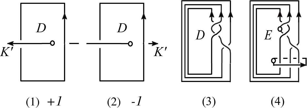
Figure 6. The sign of the intersection point: (1) +1+1 and (2) −1-1. (3) The associated disk D=D(b,1)D=D_{(b,1)} and (4) the surface E=E(b,1)E=E_{(b,1)} for a 11-increasing braid b=σ12​σ2−1∈B3b=\sigma_{1}^{2}\sigma_{2}^{-1}\in B_{3}. (E(b,1)E_{(b,1)} is a twice punctured disk in this case.)

In [HK20a], the authors introduced ii-increasing braids. In this section, we review some properties of ii-increasing braids that are needed in the later section.

Recall that π:Bn→𝔖n\pi:B_{n}\rightarrow\mathfrak{S}_{n} is the surjective homomorphism as in Section 2.4. We denote by πb\pi_{b}, the permutation π⁡(b)∈𝔖n\pi(b)\in\mathfrak{S}_{n} for b∈Bnb\in B_{n}. Suppose that b∈Bnb\in B_{n} is a braid with πb​(i)=i\pi_{b}(i)=i, i.e., the permutation πb\pi_{b} fixes the index ii. The closure cl⁡(b⁡(i))\mathrm{cl}(b(i)) of the ii-th strand b⁡(i)b(i) is a component of the closure cl⁡(b)\mathrm{cl}(b) of bb. We consider an oriented disk D=D(b,i)D=D_{(b,i)} bounded by the longitude ℓi\ell_{i} of a regular neighborhood 𝒩⁡(cl⁡(b⁡(i)))\mathcal{N}(\mathrm{cl}(b(i))) of cl⁡(b⁡(i))\mathrm{cl}(b(i)). Such a disk DD is unique up to isotopy on ℰ⁡(cl⁡(b⁡(i)))\mathcal{E}(\mathrm{cl}(b(i))). Let b−b⁡(i)∈Bn−1b-b(i)\in B_{n-1} be a braid with n−1n-1 strands obtained from bb by removing the ii-th strand b⁡(i)b(i). The braid bb is said to be ii-increasing (resp. ii-decreasing) if there exists a disk D=D(b,i)D=D_{(b,i)} as above with the following conditions (D1) and (D2).

  1. (D1)

    There exists at least one component K′K^{\prime} of cl⁡(b−b⁡(i))\mathrm{cl}(b-b(i)) such that D∩K′≠∅D\cap K^{\prime}\neq\emptyset.

  2. (D2)

    Each component of cl⁡(b−b⁡(i))\mathrm{cl}(b-b(i)) and DD intersect with each other transversally, and every intersection point has the same sign +1+1 (resp. −1-1), see Figure 6(1)(2).

We call D=D(b,i)D=D_{(b,i)} the associated disk of the pair (b,i)(b,i). Then we set

I⁡(b,i)=D∩cl⁡(b−b⁡(i)).I(b,i)=D\cap\mathrm{cl}(b-b(i)).

By (D1) we have I⁡(b,i)≠∅I(b,i)\neq\emptyset. Let u⁡(b,i)≥1u(b,i)\geq 1 be the cardinality |I⁡(b,i)||I(b,i)| of I⁡(b,i)I(b,i). We call u⁡(b,i)u(b,i) the intersection number of the pair (b,i)(b,i).

Example 2.12.
  1. (1)

    A braid b=σ12​σ2−1∈B3b=\sigma_{1}^{2}\sigma_{2}^{-1}\in B_{3} is 11-increasing with u⁡(b,1)=1u(b,1)=1. See Figure 6(3).

  2. (2)

    A pure braid b=σ14​σ2−2∈B3b=\sigma_{1}^{4}\sigma_{2}^{-2}\in B_{3} is 11-increasing with u⁡(b,1)=2u(b,1)=2 and 33-decreasing with u⁡(b,3)=1u(b,3)=1.

Properties of ii-increasing braids are given in the next two lemmas. The same properties hold for ii-decreasing braids.

Lemma 2.13.

If bb and b′b^{\prime} are ii-increasing braids with the same number of strands, then the product b​b′bb^{\prime} is also ii-increasing such that u⁡(b​b′,i)=u⁡(b,i)+u⁡(b′,i)u(bb^{\prime},i)=u(b,i)+u(b^{\prime},i).

Proof.

Let D2D^{2} be the disk with radius 11. For k=0,1,2k=0,1,2, let (D2×[0,1])k(D^{2}\times[0,1])_{k} be cylinders in S3S^{3} such that (D2×[0,1])1∩cl⁡(b)=b(D^{2}\times[0,1])_{1}\cap\mathrm{cl}(b)=b, (D2×[0,1])0∩cl⁡(b′)=b′(D^{2}\times[0,1])_{0}\cap\mathrm{cl}(b^{\prime})=b^{\prime} and (D2×[0,1])2∩cl⁡(b​b′)=b​b′(D^{2}\times[0,1])_{2}\cap\mathrm{cl}(bb^{\prime})=bb^{\prime}. We set Rθ:={r​ei​θ| 0≤r≤1}⊂D2R_{\theta}:=\{re^{i\theta}\ |\ 0\leq r\leq 1\}\subset D^{2}. We denote by DD (resp. D′D^{\prime}), an associated disk of the pair (b,i)(b,i) (resp. (b′,i)(b^{\prime},i)). By an ambient isotopy, we may assume that there exists θ0∈[0,2​π)\theta_{0}\in[0,2\pi) such that D∩(D2×[0,1])1=Rθ0×[0,1]D\cap(D^{2}\times[0,1])_{1}=R_{\theta_{0}}\times[0,1] (resp. D′∩(D2×[0,1])0=Rθ0×[0,1]D^{\prime}\cap(D^{2}\times[0,1])_{0}=R_{\theta_{0}}\times[0,1]) and D∩cl⁡(b)=Rθ0×[0,1]∩cl⁡(b)D\cap\mathrm{cl}(b)=R_{\theta_{0}}\times[0,1]\cap\mathrm{cl}(b) (resp. D′∩cl⁡(b′)=Rθ0×[0,1]∩cl⁡(b′)D^{\prime}\cap\mathrm{cl}(b^{\prime})=R_{\theta_{0}}\times[0,1]\cap\mathrm{cl}(b^{\prime})). We stuck the cylinder (D2×[0,1])1(D^{2}\times[0,1])_{1} over the cylinder (D2×[0,1])0(D^{2}\times[0,1])_{0} so that (D2×{0})1(D^{2}\times\{0\})_{1} is attached to (D2×{1})0(D^{2}\times\{1\})_{0}, and we identify the result with D2×[0,2]D^{2}\times[0,2]. Let

F:D2×[0,2]→(D2×[0,1])2F:D^{2}\times[0,2]\to(D^{2}\times[0,1])_{2}

be the homeomorphism defined by F⁡(x,t)=(x,t/2)F(x,t)=(x,t/2). Then F⁡(b∪b′)=b​b′F(b\cup b^{\prime})=bb^{\prime} by the definition of the product of braids. The image of the union of Rθ0×[0,1]R_{\theta_{0}}\times[0,1] in (D2×[0,1])1(D^{2}\times[0,1])_{1} and Rθ0×[0,1]R_{\theta_{0}}\times[0,1] in (D2×[0,1])0(D^{2}\times[0,1])_{0} under the homeomorphism FF is Rθ0×[0,1]⊂(D2×[0,1])2R_{\theta_{0}}\times[0,1]\subset(D^{2}\times[0,1])_{2}, which intersects with the closure cl⁡(b​b′)\mathrm{cl}(bb^{\prime}) of the product b​b′bb^{\prime} positively at (u⁡(b,i)+u⁡(b′,i))(u(b,i)+u(b^{\prime},i)) points. Therefore, b​b′bb^{\prime} is ii-increasing and the equality u⁡(b​b′,i)=u⁡(b,i)+u⁡(b′,i)u(bb^{\prime},i)=u(b,i)+u(b^{\prime},i) holds. ∎

Lemma 2.14.

Suppose that b∈Bnb\in B_{n} is an ii-increasing braid. Then skew⁡(b)∈Bn\mathrm{skew}(b)\in B_{n} is an (n−i+1)(n-i+1)-increasing braid such that u⁡(skew⁡(b),n−i+1)=u⁡(b,i)u(\mathrm{skew}(b),n-i+1)=u(b,i).

Proof.

The assertion follows from that fact that skew:Bn→Bn\mathrm{skew}:B_{n}\to B_{n} is induced by the involution RR on the cylinder D2×[0,1]D^{2}\times[0,1] given in Section 2.1. ∎

Example 2.15.

Let b=σ32​σ4−2b=\sigma_{3}^{2}\sigma_{4}^{-2} be the 55-braid as in Example 2.1. Then bb is 33-increasing with u⁡(b,3)=1u(b,3)=1. By Lemma 2.14, the braid skew⁡(b)=σ1−2​σ22\mathrm{skew}(b)=\sigma_{1}^{-2}\sigma_{2}^{2} is 33-increasing with u⁡(skew⁡(b),3)=1u(\mathrm{skew}(b),3)=1. Then by Lemma 2.13, the braid b~=skew⁡(b)⋅b=σ1−2​σ22​σ32​σ4−2\widetilde{b}=\mathrm{skew}(b)\cdot b=\sigma_{1}^{-2}\sigma_{2}^{2}\sigma_{3}^{2}\sigma_{4}^{-2} is also 33-increasing with u⁡(b~,3)=u⁡(skew⁡(b),3)+u⁡(b,3)=2u(\widetilde{b},3)=u(\mathrm{skew}(b),3)+u(b,3)=2.

Recall that Tb=ℰ⁡(br⁡(b))T_{b}=\mathcal{E}(\mathrm{br}(b)) is the exterior of the braided link br⁡(b)\mathrm{br}(b) and the surface FbF_{b} is a genus 00 fiber of the fibration Tb→S1T_{b}\rightarrow S^{1}. See Section 2.3. We shall define the 22-dimensional subcone C(b,i)C_{(b,i)} of H2​(Tb,∂Tb,ℝ)H_{2}(T_{b},\partial T_{b};{\mathbb{R}}) for an ii-increasing braid bb. To do this, we first consider the braided link br⁡(b)=cl⁡(b)∪A\mathrm{br}(b)=\mathrm{cl}(b)\cup A. The associated disk D=D(b,i)D=D_{(b,i)} has a unique point of intersection with AA, and the cardinality of I⁡(b,i)∪(D∩A)I(b,i)\cup(D\cap A) is u⁡(b,i)+1u(b,i)+1. To deal with br⁡(b)=cl⁡(b)∪A\mathrm{br}(b)=\mathrm{cl}(b)\cup A as an oriented link, we consider an orientation of cl⁡(b)\mathrm{cl}(b) as we described in Section 2.3, and assign an orientation of the braid axis AA of bb so that the sign of the intersection between DD and AA is +1+1 as in Figure 6(1). See Figure 3(2) for the orientation of AA of the 33-braid σ12​σ2−1\sigma_{1}^{2}\sigma_{2}^{-1} that is 11-increasing.

Next, we define an oriented surface E(b,i)E_{(b,i)} of genus 00 embedded in TbT_{b}. Consider small u⁡(b,i)+1u(b,i)+1 disks in the associated disk D=D(b,i)D=D_{(b,i)} whose centers are points of I⁡(b,i)∪(D∩A)I(b,i)\cup(D\cap A). Then E(b,i)E_{(b,i)} is a surface of genus 00 with u⁡(b,i)+2u(b,i)+2 boundary components obtained from DD by removing the interiors of those small disks. We choose the orientation of E(b,i)E_{(b,i)} so that it agrees with the orientation of DD. See Figure 6(4).

Lastly, we define the 22-dimensional subcone C(b,i)C_{(b,i)} of H2​(Tb,∂Tb,ℝ)H_{2}(T_{b},\partial T_{b};{\mathbb{R}}) spanned by the two integral classes [Fb][F_{b}] and [E(b,i)][E_{(b,i)}] as follows.

(2.3) C(b,i)={x[Fb]+y[E(b,i)]|x>0,y>0}.C_{(b,i)}=\{x[F_{b}]+y[E_{(b,i)}]\ |\ x>0,\ y>0\}.

We write (x,y)=x⁡[Fb]+y⁡[E(b,i)]∈C(b,i)(x,y)=x[F_{b}]+y[E_{(b,i)}]\in C_{(b,i)}. The Thurston norm of (x,y)(x,y) is denoted by ‖(x,y)‖\|(x,y)\|.

Theorem 2.16 ([HK20a]).

Let bb be an ii-increasing braid. Suppose that bb is pseudo-Anosov. Let 𝒞\mathscr{C} be the fibered cone of the 33-manifold TbT_{b} containing [Fb]=(1,0)∈C(b,i)[F_{b}]=(1,0)\in C_{(b,i)}. Then we have the following.

  1. (1)

    C(b,i)⊂𝒞C_{(b,i)}\subset\mathscr{C}.

  2. (2)

    The fiber F(x,y)F_{(x,y)} for each primitive integral class (x,y)∈C(b,i)(x,y)\in C_{(b,i)} has genus 00.

  3. (3)

    Let ϕ(x,y):F(x,y)→F(x,y)\phi_{(x,y)}:F_{(x,y)}\rightarrow F_{(x,y)} denote the monodromy of the fibration Tb→S1T_{b}\rightarrow S^{1} associated with a primitive integral class (x,y)∈C(b,i)(x,y)\in C_{(b,i)}. Then there exists a jj-increasing braid b(x,y)∈B‖(x,y)‖+1b_{(x,y)}\in B_{\|(x,y)\|+1} for some index j=j(x,y)j=j_{(x,y)} which gives the monodromy ϕ(x,y):F(x,y)→F(x,y)\phi_{(x,y)}:F_{(x,y)}\rightarrow F_{(x,y)}.

The proof of Theorem 2.16(1)(2) can be found in Theorem 3.2(1)(2) in [HK20a]. The statement of Theorem 2.16(3) follows from the argument in the proof of Theorem 3.2(3) in [HK20a].

3. Braids increasing in the middle

Let bb be a braid with 2​n+12n+1 strands. Then the notion ‘ii-increasing braid’ makes sense for i=1,…,2​n+1i=1,\dots,2n+1. (See Section 2.7.) In this section, we restrict our attention to the case i=n+1i=n+1: Suppose that bb is an (n+1)(n+1)-increasing braid. In this case we say that bb is increasing in the middle. We write Cb:=C(b,n+1)C_{b}:=C_{(b,n+1)} for the subcone of H2​(Tb,∂Tb,ℝ)H_{2}(T_{b},\partial T_{b};{\mathbb{R}}). (See (2.3) for the definition of the subcone.) Then b∙∈B2​nb^{\bullet}\in B_{2n} denotes the braid obtained from b∈B2​n+1b\in B_{2n+1} by removing the strand of the middle index n+1n+1.

Example 3.1.

(cf. Example 2.15) Suppose that b∈B2​n+1b\in B_{2n+1} is a braid increasing in the middle. By Lemma 2.14, the braid skew⁡(b)\mathrm{skew}(b) is increasing in the middle. By Lemma 2.13 the braid b~=skew⁡(b)⋅b\widetilde{b}=\mathrm{skew}(b)\cdot b is also increasing in the middle with the intersection number

u⁡(b~,n+1)=u⁡(skew⁡(b),n+1)+u⁡(b,n+1)=2​u​(b,n+1).u(\widetilde{b},n+1)=u(\mathrm{skew}(b),n+1)+u(b,n+1)=2u(b,n+1).

The skew-palindromization (b∙)~\widetilde{(b^{\bullet})} of b∙b^{\bullet} satisfies

(b∙)~=skew⁡(b∙)​b∙=(b~)∙,\widetilde{(b^{\bullet})}=\mathrm{skew}(b^{\bullet})b^{\bullet}=(\widetilde{b})^{\bullet},

i.e., (b∙)~∈B2​n\widetilde{(b^{\bullet})}\in B_{2n} is obtained from the skew-palindromization b~\widetilde{b} of bb by removing the strand of the middle index n+1n+1. Hereafter we simply denote the braid (b∙)~\widetilde{(b^{\bullet})} by b∙~\widetilde{b^{\bullet}}. Applying Theorem 2.8 to the circular plat closure L=C⁡(b∙)L=C(b^{\bullet}) of b∙∈B2​nb^{\bullet}\in B_{2n}, we have 𝔱⁡(b∙~)∈𝒟n−1​(MC⁡(b∙))\mathfrak{t}(\widetilde{b^{\bullet}})\in\mathcal{D}_{n-1}(M_{C(b^{\bullet})}).

Example 3.2.

The half twist Δ=Δ2​n+1∈B2​n+1\Delta=\Delta_{2n+1}\in B_{2n+1} is a braid increasing in the middle with u⁡(Δ,n+1)=nu(\Delta,n+1)=n. By Lemma 2.13 the positive power Δp\Delta^{p} for p≥1p\geq 1 is a braid increasing in the middle, and it holds

u⁡(Δp,n+1)=p⋅u⁡(Δ,n+1)=p​n.u(\Delta^{p},n+1)=p\cdot u(\Delta,n+1)=pn.

The braid Δ∙∈B2​n\Delta^{\bullet}\in B_{2n} satisfies Δ∙=Δ2​n∈B2​n\Delta^{\bullet}=\Delta_{2n}\in B_{2n}, i.e., Δ∙\Delta^{\bullet} is equal to the half twist Δ2​n\Delta_{2n} with 2​n2n strands.

Refer to caption
Figure 7. (1) The subcone Cβ~=C(β~,n+1)C_{\widetilde{\beta}}=C_{(\widetilde{\beta},n+1)} spanned by [F][F] and [E][E], where F:=Fβ~F:=F_{\widetilde{\beta}} and E:=E(β~,n+1)E:=E_{(\widetilde{\beta},n+1)}. (Primitive integral classes (1,1),(2,1),…,(k,1),…(1,1),(2,1),\dots,(k,1),\dots are indicated.) (2) The braided link br⁡(β~)\mathrm{br}(\widetilde{\beta}) of β~=σ1​σ22​σ32​σ4∈B5\widetilde{\beta}=\sigma_{1}\sigma_{2}^{2}\sigma_{3}^{2}\sigma_{4}\in B_{5}.

Given a braid β∈B2​n+1\beta\in B_{2n+1} increasing in the middle, we suppose that the skew-palindromization β~\widetilde{\beta} of β\beta is pseudo-Anosov. Consider the subcone Cβ~=C(β~,n+1)C_{\widetilde{\beta}}=C_{(\widetilde{\beta},n+1)} of H2​(Tβ~,∂Tβ~,ℝ)H_{2}(T_{\widetilde{\beta}},\partial T_{\widetilde{\beta}};{\mathbb{R}}) for the hyperbolic 33-manifold Tβ~T_{\widetilde{\beta}} (Figure 7(1)). We now apply Theorem 2.16 for the skew-palindromization β~\widetilde{\beta}. For the class (1,0)=[Fβ~]∈Cβ~(1,0)=[F_{\widetilde{\beta}}]\in C_{\widetilde{\beta}}, the monodromy ϕ(1,0):F(1,0)→F(1,0)\phi_{(1,0)}:F_{(1,0)}\rightarrow F_{(1,0)} defined on the fiber F(1,0)=Fβ~F_{(1,0)}=F_{\widetilde{\beta}} is given by the braid β~\widetilde{\beta} that is increasing in the middle. The following result (Theorem 3.4) tells us that this property is inherited for all primitive classes (x,y)∈Cβ~⊂𝒞(x,y)\in C_{\widetilde{\beta}}\subset\mathscr{C}, where 𝒞\mathscr{C} is the fibered cone of Tβ~T_{\widetilde{\beta}} containing [Fβ~]∈Cβ~[F_{\widetilde{\beta}}]\in C_{\widetilde{\beta}}.

Example 3.3.

Consider the braid β=σ32​σ4∈B5\beta=\sigma_{3}^{2}\sigma_{4}\in B_{5}. The braid β\beta is increasing in the middle. The skew-palindromization β~=σ1​σ22​σ32​σ4∈B5\widetilde{\beta}=\sigma_{1}\sigma_{2}^{2}\sigma_{3}^{2}\sigma_{4}\in B_{5} is pseudo-Anosov, see the proof of Step 1 in [HK20a, Proof of Theorem D]. See Figure 7(2) for the braided link.

Theorem 3.4.

Let β∈B2​n+1\beta\in B_{2n+1} be a braid increasing in the middle. Suppose that the skew-palindromization β~\widetilde{\beta} of β\beta is pseudo-Anosov. Let (x,y)∈Cβ~(x,y)\in C_{\widetilde{\beta}} be a primitive integral class. Then we have the following.

  1. (1)

    There exists a braid α(x,y)∈B‖(x,y)‖+1\alpha_{(x,y)}\in B_{\|(x,y)\|+1} increasing in the middle such that the monodromy ϕ(x,y):F(x,y)→F(x,y)\phi_{(x,y)}:F_{(x,y)}\rightarrow F_{(x,y)} of the fibration Tβ~→S1T_{\widetilde{\beta}}\rightarrow S^{1} associated with (x,y)(x,y) is given by the skew-palindromization α(x,y)~\widetilde{\alpha_{(x,y)}} of α(x,y)\alpha_{(x,y)}. (In particular α(x,y)~\widetilde{\alpha_{(x,y)}} is a pseudo-Anosov braid.)

  2. (2)

    Let α(x,y)∙∈B‖(x,y)‖\alpha_{(x,y)}^{\bullet}\in B_{\|(x,y)\|} be the braid obtained from α(x,y)\alpha_{(x,y)} by removing the strand of the middle index. Then C⁡(β∙)=C⁡(α(x,y)∙)C(\beta^{\bullet})=C(\alpha_{(x,y)}^{\bullet}), and hence 𝔱⁡(α(x,y)∙~)∈𝒟‖(x,y)‖2−1​(MC⁡(β∙))\mathfrak{t}(\widetilde{\alpha_{(x,y)}^{\bullet}})\in\mathcal{D}_{\frac{\|(x,y)\|}{2}-1}(M_{C(\beta^{\bullet})}).

For the proof of Theorem 3.4, we need some preparations from [HK20a]. Let LL be a link in S3S^{3}. Suppose that an unknot KK is a component of LL. Then the exterior ℰ⁡(K)\mathcal{E}(K) is a solid torus (resp. the boundary of the exterior ∂ℰ⁡(K)\partial\mathcal{E}(K) is a torus). We take a disk DD bounded by the longitude of a tubular neighborhood 𝒩⁡(K)\mathcal{N}(K) of KK. We define a mapping class tDt_{D} defined on ℰ⁡(K)\mathcal{E}(K) as follows. We cut ℰ⁡(K)\mathcal{E}(K) along DD. We have resulting two sides obtained from DD, and reglue two sides by twisting 360360 degrees so that the mapping class defined on the torus ∂ℰ⁡(K)\partial\mathcal{E}(K) is the right-handed Dehn twist about ∂D\partial D. We call such a mapping class tDt_{D} on ℰ⁡(K)\mathcal{E}(K) the disk twist about DD. For simplicity, we also call a representative of the mapping class tDt_{D} the disk twist about DD, and denote it by the same notation

tD:ℰ⁡(K)→ℰ⁡(K).t_{D}:\mathcal{E}(K)\rightarrow\mathcal{E}(K).

For any integer ℓ\ell, consider the homeomorphism

tDℓ:ℰ⁡(K)→ℰ⁡(K).t_{D}^{\ell}:\mathcal{E}(K)\rightarrow\mathcal{E}(K).

Observe that tDℓt_{D}^{\ell} converts the link LL into a link K∪tDℓ​(L−K)K\cup t_{D}^{\ell}(L-K) so that S3∖LS^{3}\setminus L is homeomorphic to S3∖(K∪tDℓ​(L−K))S^{3}\setminus(K\cup t_{D}^{\ell}(L-K)). Then tDℓt_{D}^{\ell} induces a homeomorphism hD,ℓh_{D,\ell} between the exteriors of links LL and K∪tDℓ​(L−K)K\cup t_{D}^{\ell}(L-K):

hD,ℓ:ℰ⁡(L)→ℰ⁡(K∪tDℓ​(L−K)).h_{D,\ell}:\mathcal{E}(L)\rightarrow\mathcal{E}(K\cup t_{D}^{\ell}(L-K)).

Consider the braided link L=br⁡(b)=A∪cl⁡(b)L=\mathrm{br}(b)=A\cup\mathrm{cl}(b) for a braid bb with the braid axis AA. We consider the kk-th power of the disk twist about the disk DAD_{A} bounded by the longitude of 𝒩⁡(A)\mathcal{N}(A):

tDAk:ℰ⁡(A)→ℰ⁡(A).t_{D_{A}}^{k}:\mathcal{E}(A)\rightarrow\mathcal{E}(A).

Note that A∪tDAk​(cl⁡(b))=A∪cl⁡(b​Δ2​k)=br⁡(b​Δ2​k)A\cup t_{D_{A}}^{k}(\mathrm{cl}(b))=A\cup\mathrm{cl}(b\Delta^{2k})=\mathrm{br}(b\Delta^{2k}). Hence hDA,kh_{D_{A},k} sends ℰ⁡(br⁡(b))=ℰ⁡(A∪cl⁡(b))\mathcal{E}(\mathrm{br}(b))=\mathcal{E}(A\cup\mathrm{cl}(b)) to ℰ⁡(br⁡(b​Δ2​k))=ℰ⁡(A∪cl⁡(b​Δ2​k))\mathcal{E}(\mathrm{br}(b\Delta^{2k}))=\mathcal{E}(A\cup\mathrm{cl}(b\Delta^{2k})).

Following [HK20a, Section 4.1], we next introduce a sequence of braided links {br⁡(bp)}p=1∞\{\mathrm{br}(b_{p})\}_{p=1}^{\infty} obtained from an ii-increasing braid b∈Bnb\in B_{n} such that Tbp≃TbT_{b_{p}}\simeq T_{b} i.e., the mapping tori TbpT_{b_{p}} and TbT_{b} are homeomorphic to each other for each p≥1p\geq 1. We set u=u⁡(b,i)u=u(b,i) that is the intersection number of the pair (b,i)(b,i). Let DD be an associated disk of the pair (b,i)(b,i). We take a disk twist

tD:ℰ⁡(cl⁡(b⁡(i)))→ℰ⁡(cl⁡(b⁡(i)))t_{D}:\mathcal{E}(\mathrm{cl}(b(i)))\rightarrow\mathcal{E}(\mathrm{cl}(b(i)))

so that the point of intersection D∩AD\cap A becomes the center of the twisting about DD, i.e., tD​(D∩A)=D∩At_{D}(D\cap A)=D\cap A. It follows that

tD​(br⁡(b−b⁡(i)))∪cl⁡(b⁡(i))t_{D}(\mathrm{br}(b-b(i)))\cup\mathrm{cl}(b(i))

is a braided link of a jj-increasing braid for some index jj with (n+u)(n+u) strands. (cf. Figures 11 and 12 in [HK20a].) We define b1b_{1} to be such a braid with (n+u)(n+u) strands. The trivial knot tD​(A)(=A)t_{D}(A)(=A) becomes a braid axis of b1b_{1}. By definition of the disk twist, we have Tb1≃TbT_{b_{1}}\simeq T_{b}. We remark that there is some ambiguity in defining b1b_{1}. However the braid b1b_{1} is well defined up to conjugate, see [HK20a, Section 4.1]. The conjugacy class of b1b_{1} is denoted by ⟨b1⟩\langle b_{1}\rangle.

To define the braid bpb_{p} obtained from the above bb for p≥1p\geq 1, we consider the pp-th power

tDp:ℰ⁡(cl⁡(b⁡(i)))→ℰ⁡(cl⁡(b⁡(i)))t_{D}^{p}:\mathcal{E}(\mathrm{cl}(b(i)))\rightarrow\mathcal{E}(\mathrm{cl}(b(i)))

using the above disk twist tDt_{D}. As in the case of p=1p=1,

tDp​(br⁡(b−b⁡(i)))∪cl⁡(b⁡(i))t_{D}^{p}(\mathrm{br}(b-b(i)))\cup\mathrm{cl}(b(i))

is a braided link of an increasing braid for some index with (n+p​u)(n+pu) strands. We define bp∈Bn+p​ub_{p}\in B_{n+pu} to be such a braid with n+p​un+pu strands. Then Tbp≃TbT_{b_{p}}\simeq T_{b}. As in the case of p=1p=1, the braid bpb_{p} is well defined up to conjugate. We denote by ⟨bp⟩\langle b_{p}\rangle, the conjugacy class of such a braid bpb_{p}. We say that ⟨bp⟩\langle b_{p}\rangle (or a representative bpb_{p}) is obtained from bb by the disk twist tDt_{D} (pp times).

Now we suppose that a braid bb is of the form b=β~b=\widetilde{\beta}, where β∈B2​n+1\beta\in B_{2n+1} is a braid increasing in the middle. Then β~\widetilde{\beta} is also increasing in the middle. The following lemma describes a property of a representative of the conjugacy class ⟨(β~)p⟩\langle(\widetilde{\beta})_{p}\rangle obtained from β~\widetilde{\beta} by the disk twist pp times.

Lemma 3.5.

Let β∈B2​n+1\beta\in B_{2n+1} be a braid increasing in the middle with the intersection number u=u⁡(β,n+1)u=u(\beta,n+1). We consider the skew-palindromization β~\widetilde{\beta} (that is increasing in the middle). Let ⟨(β~)p⟩\langle(\widetilde{\beta})_{p}\rangle be the conjugacy class of a braid obtained from β~\widetilde{\beta} by the disk twist pp times for p≥1p\geq 1. We have the following.

  1. (1)

    There exists a braid α=α⁡(p)∈B2​n+2​p​u+1\alpha=\alpha(p)\in B_{2n+2pu+1} increasing in the middle such that α~=α⁡(p)~∈⟨(β~)p⟩\widetilde{\alpha}=\widetilde{\alpha(p)}\in\langle(\widetilde{\beta})_{p}\rangle, i.e., α~=α⁡(p)~\widetilde{\alpha}=\widetilde{\alpha(p)} represents the conjugacy class ⟨(β~)p⟩\langle(\widetilde{\beta})_{p}\rangle.

  2. (2)

    C⁡(β∙)=C⁡(α∙)C(\beta^{\bullet})=C(\alpha^{\bullet}), where α∙=α​(p)∙∈B2​n+2​p​u\alpha^{\bullet}=\alpha(p)^{\bullet}\in B_{2n+2pu}.

  3. (3)

    𝔱⁡(α∙~)∈𝒟g​(MC⁡(β∙))\mathfrak{t}(\widetilde{\alpha^{\bullet}})\in\mathcal{D}_{g}(M_{C(\beta^{\bullet})}), where g=n+p​u−1g=n+pu-1.

Refer to caption
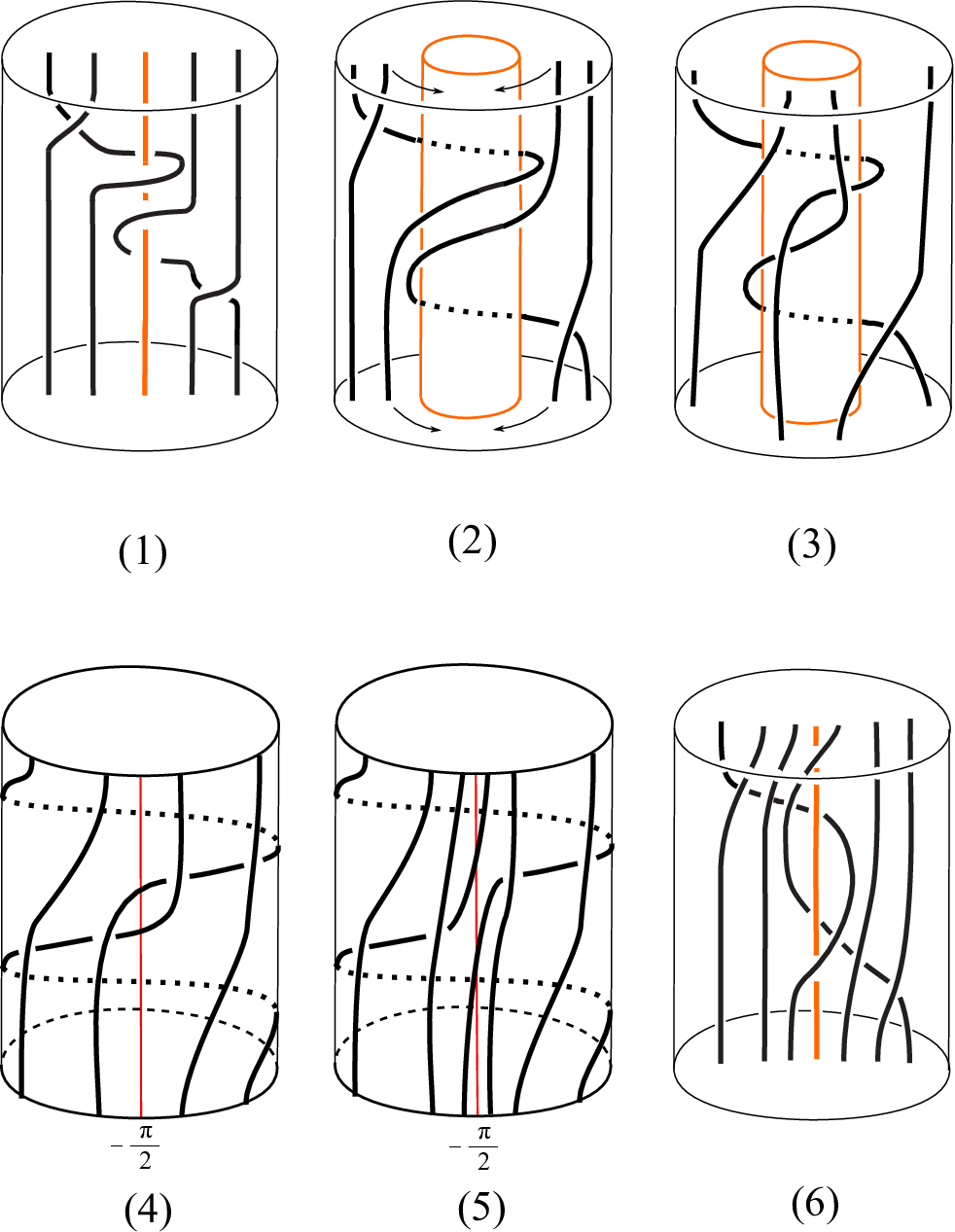
Figure 8. (1) The skew-palindromization β~\widetilde{\beta} of β=σ32​σ4∈B5\beta=\sigma_{3}^{2}\sigma_{4}\in B_{5}. (2) The regular neighborhood of the middle strand (third strand) is removed. (3) The base points are moved to the circle {12​ei​θ| 0≤θ≤2​π}\{\frac{1}{2}e^{i\theta}\,|\,0\leq\theta\leq 2\pi\}. (4) Project cl⁡(β∙~)\mathrm{cl}(\widetilde{\beta^{\bullet}}) to the torus. (5) Dehn twist about the circle c={−π2}×[0,1]c=\{-\frac{\pi}{2}\}\times[0,1] on the torus. (6) The skew-palindromization α⁡(1)~\widetilde{\alpha(1)} of α⁡(1)=σ3​σ4​σ5​σ6​σ3∈B7\alpha(1)=\sigma_{3}\sigma_{4}\sigma_{5}\sigma_{6}\sigma_{3}\in B_{7}. (cf. Figure 7 in [HK20b].)
Refer to caption
Figure 9. The braid β∙∈B2​n\beta^{\bullet}\in B_{2n} consists of b1b_{1}, b2b_{2} and slanted parallel arcs between them. The disk twist tDt_{D} induces a Dehn twist about c={−π2}×[0,1]c=\{-\frac{\pi}{2}\}\times[0,1] on the torus. Compare Figure 8(4)(5) with Figure 9.
Proof.

(1) Figure 8 illustrates the procedure of the proof. (See also Example 3.3.) We put cl⁡(β~)\mathrm{cl}(\widetilde{\beta}) in D2×S1D^{2}\times S^{1} =D2×([0,1]/0∼1)=D^{2}\times([0,1]/0\sim 1) such that cl⁡(β~)∩D2×[0,1/2]\mathrm{cl}(\widetilde{\beta})\cap D^{2}\times[0,1/2] =β=\beta, cl⁡(β~)∩D2×[1,1/2]\mathrm{cl}(\widetilde{\beta})\cap D^{2}\times[1,1/2] =skew⁡(β)=\mathrm{skew}(\beta) and cl​(β~​(n+1))\mathrm{cl}(\widetilde{\beta}(n+1)) corresponds to (the center of ​D2)×S1(\text{the center of }D^{2})\times S^{1}, as shown in (1) of Figure 8. Let RD2×S1:D2×S1→D2×S1R_{D^{2}\times S^{1}}:D^{2}\times S^{1}\to D^{2}\times S^{1} be the involution induced by the involution R⁡(r​ei​θ,t)=(r​ei⁡(π−θ),1−t)R(re^{i\theta},t)=(re^{i(\pi-\theta)},1-t) on D2×[0,1]D^{2}\times[0,1]. Let 𝒩\mathcal{N} be the tubular neighborhood of (the center of ​D2)×S1(\text{the center of }D^{2})\times S^{1} such that cl⁡(β~)∩(D2×S1∖int​𝒩)\mathrm{cl}(\widetilde{\beta})\cap(D^{2}\times S^{1}\setminus\mathrm{int}\,\mathcal{N}) == cl⁡(β∙~)\mathrm{cl}(\widetilde{{\beta}^{\bullet}}), as shown in (2) of Figure 8. We identify D2×S1∖int​𝒩D^{2}\times S^{1}\setminus\mathrm{int}\,\mathcal{N} with [0,1]×S1×S1=[0,1]×([0,2​π]/0∼2​π)×([0,1]/0∼1)[0,1]\times S^{1}\times S^{1}=[0,1]\times([0,2\pi]/0\sim 2\pi)\times([0,1]/0\sim 1) so that ∂𝒩={0}×S1×S1\partial\mathcal{N}=\{0\}\times S^{1}\times S^{1}, {12​ei​θ| 0≤θ≤2​π}×{pt}={12}×S1×{pt}\{\frac{1}{2}e^{i\theta}\,|\,0\leq\theta\leq 2\pi\}\times\{\mathrm{pt}\}=\{\frac{1}{2}\}\times S^{1}\times\{\mathrm{pt}\}, and for the disk DD associated to the pair (β~,n+1)(\widetilde{\beta},n+1), we have (D2×S1∖int​𝒩)∩D=[0,1]×{−π2}×S1(D^{2}\times S^{1}\setminus\mathrm{int}\,\mathcal{N})\cap D=[0,1]\times\{-\frac{\pi}{2}\}\times S^{1}. We deform cl⁡(β∙~)\mathrm{cl}(\widetilde{\beta^{\bullet}}) so as to intersect D2×{0}D^{2}\times\{0\} in 2​n2n points {12ei​θ|θ=−12​n+2π,−22​n+2π,…,−n2​n+2π,−n+22​n+2π,−n+32​n+2π,…,−2​n+12​n+2π}\{\frac{1}{2}e^{i\theta}|\theta=-\frac{1}{2n+2}\pi,-\frac{2}{2n+2}\pi,\ldots,-\frac{n}{2n+2}\pi,-\frac{n+2}{2n+2}\pi,-\frac{n+3}{2n+2}\pi,\ldots,-\frac{2n+1}{2n+2}\pi\} and not to occur new intersections with [0,1]×{−π2}×S1[0,1]\times\{-\frac{\pi}{2}\}\times S^{1} by the isotopy commuting with the involution RR, as shown in (3) of Figure 8. We make a projection 𝒟⁡(cl⁡(β∙~))\mathcal{D}(\mathrm{cl}(\widetilde{\beta^{\bullet}})) of cl⁡(β∙~)\mathrm{cl}(\widetilde{\beta^{\bullet}}) onto {12}×S1×S1\{\frac{1}{2}\}\times S^{1}\times S^{1} with at most double points, and each double point indicates which is over pass or under pass in the same way as a knot diagram, as shown in (4) of Figure 8. For short, we drop {12}\{\frac{1}{2}\} from {12}×S1×S1\{\frac{1}{2}\}\times S^{1}\times S^{1} and identify it with a torus S1×S1=([−32π,12π]/−32π∼12π)×([0,1]/0∼1)S^{1}\times S^{1}=([-\frac{3}{2}\pi,\frac{1}{2}\pi]/-\frac{3}{2}\pi\sim\frac{1}{2}\pi)\times([0,1]/0\sim 1). With this identification, the restriction of RR on {12}×S1×S1\{\frac{1}{2}\}\times S^{1}\times S^{1} is an involution which maps (θ,t)(\theta,t) to (−π−θ,1−t)(-\pi-\theta,1-t), i.e., a π\pi-rotation about (−π2,12)(-\frac{\pi}{2},\frac{1}{2}). Since β\beta is an increasing braid in the middle, 𝒟⁡(cl⁡(β∙~))\mathcal{D}(\mathrm{cl}(\widetilde{\beta^{\bullet}})) intersects −π2×[12,1]-\frac{\pi}{2}\times[\frac{1}{2},1] in u=u⁡(β,n+1)u=u(\beta,n+1) points and −π2×[0,12]-\frac{\pi}{2}\times[0,\frac{1}{2}] in u=u⁡(β,n+1)u=u(\beta,n+1) points as shown in Figure 9. The disk twist tDt_{D} induces the Dehn twist about the circle c={−π2}×[0,1]c=\{-\frac{\pi}{2}\}\times[0,1] in S1×S1S^{1}\times S^{1} which commutes with R|S1×S1R|_{S^{1}\times S^{1}}. This Dehn twist changes 𝒟⁡(cl⁡(β∙~))\mathcal{D}(\mathrm{cl}(\widetilde{\beta^{\bullet}})) as shown in the right of Figure 9 and (5) of Figure 8. Now we append (the center of ​D2)×S1(\text{the center of }D^{2})\times S^{1} to the above result, that is, append an under-going string {−π2}×[0,1]\{-\frac{\pi}{2}\}\times[0,1] in the right of Figure 9 and regard the new diagram as a closure of the planar braid, as shown in (6) of Figure 8. Let α⁡(p)\alpha(p) be the braid indicated by the lower part of the result. Then the upper part corresponds to skew⁡(α⁡(p))\mathrm{skew}(\alpha(p)), and hence α⁡(p)~\widetilde{\alpha(p)} is a representative of ⟨β~p⟩\langle\widetilde{\beta}_{p}\rangle. The proof of (1) is done.

(2) Let b∈B2​g+2b\in B_{2g+2} and f:S1×S1→S1×S1f:S^{1}\times S^{1}\rightarrow S^{1}\times S^{1} be the same notations as in [HK20b, p.1811]. Let γ\gamma (resp. bfb_{f}) be a braid on the annulus in the assumption (∗)(*) (resp. the assumption (∗∗)(**)) in [HK20b, p.1811]. We set b:=β∙b:=\beta^{\bullet} and f:=(tc)pf:=(t_{c})^{p}. Then bf=α​(p)∙(=α∙)b_{f}=\alpha(p)^{\bullet}(=\alpha^{\bullet}) and γ=α​(p)∙~(=α∙~)\gamma=\widetilde{\alpha(p)^{\bullet}}(=\widetilde{\alpha^{\bullet}}) satisfy the assumptions (∗)(*) and (∗∗)(**) in [HK20b, p.1811]. By Lemma 4 of [HK20b], we conclude that C⁡(β∙)C(\beta^{\bullet}) and C⁡(α∙)C(\alpha^{\bullet}) are ambient isotopic. This completes the proof of (2).

(3) The claim (3) holds from the claim (2) and Theorem 2.8. This completes the proof of Lemma 3.5. ∎

Remark 3.6.

The proof of Lemma 3.5 tells us that one can describe the braid α⁡(p)\alpha(p) in Lemma 3.5 concretely. In fact it is possible to read off α⁡(p)\alpha(p) from Figure 9. For example, in the case β=σ32​σ4∈B5\beta=\sigma_{3}^{2}\sigma_{4}\in B_{5} as in Figure 8(1), the representative α⁡(p)~∈⟨(β~)p⟩\widetilde{\alpha(p)}\in\langle(\widetilde{\beta})_{p}\rangle is the skew-palindromization of the braid α⁡(p)=σ3​σ4​…​σ4+2​p​σ2+p∈B5+2​p\alpha(p)=\sigma_{3}\sigma_{4}\dots\sigma_{4+2p}\sigma_{2+p}\in B_{5+2p} that is increasing in the middle.

Let β∈B2​n+1\beta\in B_{2n+1} be the braid increasing in the middle with the intersection number u=u⁡(β,n+1)u=u(\beta,n+1) as before. By Lemma 2.13 and Example 3.2, the product β​Δk∈B2​n+1\beta\Delta^{k}\in B_{2n+1} of β\beta and Δk\Delta^{k} for k≥1k\geq 1 is also increasing in the middle such that

u⁡(β​Δk,n+1)=u⁡(β,n+1)+u⁡(Δk,n+1)=u+k​n.u(\beta\Delta^{k},n+1)=u(\beta,n+1)+u(\Delta^{k},n+1)=u+kn.

Consider the skew-palindromization β​Δk~\widetilde{\beta\Delta^{k}} of β​Δk\beta\Delta^{k}. Recall that skew⁡(Δ)=Δ\mathrm{skew}(\Delta)=\Delta (see Section 2.1), and hence skew⁡(Δk)=Δk\mathrm{skew}(\Delta^{k})=\Delta^{k}. Thus it follows that

β​Δk~=skew⁡(β​Δk)​β​Δk=skew⁡(Δk)​skew​(β)​β​Δk=Δk​β~​Δk.\widetilde{\beta\Delta^{k}}=\mathrm{skew}(\beta\Delta^{k})\beta\Delta^{k}=\mathrm{skew}(\Delta^{k})\mathrm{skew}(\beta)\beta\Delta^{k}=\Delta^{k}\widetilde{\beta}\Delta^{k}.

By Examples 3.1 and 3.2, β​Δk~\widetilde{\beta\Delta^{k}} is a braid increasing in the middle with u⁡(β​Δk~,n+1)=2​u​(β​Δk,n+1)=2​u+2​k​n.u(\widetilde{\beta\Delta^{k}},n+1)=2u(\beta\Delta^{k},n+1)=2u+2kn. Since Δk​β~​Δk\Delta^{k}\widetilde{\beta}\Delta^{k} is conjugate to β~​Δ2​k\widetilde{\beta}\Delta^{2k} in B2​n+1B_{2n+1}, we have

br⁡(β​Δk~)=br⁡(Δk​β~​Δk)=br⁡(β~​Δ2​k).\mathrm{br}(\widetilde{\beta\Delta^{k}})=\mathrm{br}(\Delta^{k}\widetilde{\beta}\Delta^{k})=\mathrm{br}(\widetilde{\beta}\Delta^{2k}).
Lemma 3.7.

Let β∈B2​n+1\beta\in B_{2n+1} be a braid increasing in the middle with the intersection number u=u⁡(β,n+1)u=u(\beta,n+1). For k≥1k\geq 1, we consider β​Δk∈B2​n+1\beta\Delta^{k}\in B_{2n+1} and its skew-palindromization β​Δk~\widetilde{\beta\Delta^{k}}. Let ⟨(β​Δk~)p⟩\langle(\widetilde{\beta\Delta^{k}})_{p}\rangle be the conjugacy class of a braid obtained from β​Δk~\widetilde{\beta\Delta^{k}} by the disk twist pp times for p≥1p\geq 1. We have the following.

  1. (1)

    There exists a braid γ=γ⁡(k,p)∈B2​n+1+p⁡(2​u+2​k​n)\gamma=\gamma(k,p)\in B_{2n+1+p(2u+2kn)} increasing in the middle such that γ~=γ⁡(k,p)~∈⟨(β​Δk~)p⟩\widetilde{\gamma}=\widetilde{\gamma(k,p)}\in\langle(\widetilde{\beta\Delta^{k}})_{p}\rangle.

  2. (2)

    C⁡(β∙)=C⁡(γ∙)C(\beta^{\bullet})=C(\gamma^{\bullet}), where γ∙=γ​(k,p)∙∈B2​n+p⁡(2​u+2​k​n)\gamma^{\bullet}=\gamma(k,p)^{\bullet}\in B_{2n+p(2u+2kn)}.

  3. (3)

    𝔱⁡(γ∙~)∈𝒟g​(MC⁡(β∙))\mathfrak{t}(\widetilde{\gamma^{\bullet}})\in\mathcal{D}_{g}(M_{C(\beta^{\bullet})}) for g=n+p​u+p​k​n−1≡p​u−1(modn)g=n+pu+pkn-1\equiv pu-1\pmod{n}.

Proof.

Recall that for each k≥1k\geq 1, β​Δk∈B2​n+1\beta\Delta^{k}\in B_{2n+1} is a braid increasing in the middle with the intersection number u⁡(β​Δk,n+1)=u+k​nu(\beta\Delta^{k},n+1)=u+kn. The claim (1) follows immediately from Lemma 3.5(1). For the proof of the claim (2), note that

(β​Δk)∙=β∙​(Δk)∙=β∙​Δ2​nk∈B2​n,(\beta\Delta^{k})^{\bullet}=\beta^{\bullet}(\Delta^{k})^{\bullet}=\beta^{\bullet}\Delta_{2n}^{k}\in B_{2n},

see Example 3.2. Thus C⁡((β​Δk)∙)=C⁡(β∙​Δ2​nk)=C⁡(β∙)C((\beta\Delta^{k})^{\bullet})=C(\beta^{\bullet}\Delta_{2n}^{k})=C(\beta^{\bullet}), see (2.1) in Section 2.3 for the second equality. By Lemma 3.5(2), we have C⁡((β​Δk)∙)=C⁡(γ∙)C((\beta\Delta^{k})^{\bullet})=C(\gamma^{\bullet}). Putting them together, we obtain C⁡(β∙)=C⁡(γ∙)C(\beta^{\bullet})=C(\gamma^{\bullet}). The proof of (2) is done. The claim (3) holds from the claim (2) and Theorem 2.8. This completes the proof. ∎

We are now ready to prove Theorem 3.4.

Proof of Theorem 3.4.

By the assumption of Theorem 3.4, β~\widetilde{\beta} is pseudo-Anosov, and it is increasing in the middle. By Theorem 2.16(1)(2), the subcone Cβ~=C(β~,n+1)C_{\widetilde{\beta}}=C_{(\widetilde{\beta},n+1)} is a subset of the fibered cone 𝒞\mathscr{C} containing [Fβ~][F_{\widetilde{\beta}}]. Moreover the fiber F(x,y)F_{(x,y)} for each primitive integral class (x,y)∈Cβ~(x,y)\in C_{\widetilde{\beta}} has genus 00.

Let D=D(β~,n+1)D=D_{(\widetilde{\beta},n+1)} be the associated disk of the braid β~\widetilde{\beta} increasing in the middle. We consider two types of the disk twists. One is tDAk:ℰ⁡(A)→ℰ⁡(A)t_{D_{A}}^{k}:\mathcal{E}(A)\rightarrow\mathcal{E}(A) for the braid axis AA of β~\widetilde{\beta}, and the other is tDp:ℰ⁡(cl⁡(β~​(n+1)))→ℰ⁡(cl⁡(β~​(n+1)))t_{D}^{p}:\mathcal{E}(\mathrm{cl}(\widetilde{\beta}(n+1)))\rightarrow\mathcal{E}(\mathrm{cl}(\widetilde{\beta}(n+1))), where β~​(n+1)\widetilde{\beta}(n+1) is the middle strand of the (2​n+1)(2n+1)-braid β~\widetilde{\beta}. Consider the homeomorphisms

hDA,k\displaystyle h_{D_{A},k} :\displaystyle: ℰ⁡(br⁡(β~))→ℰ⁡(br⁡(β~​Δ2​k))=ℰ⁡(br⁡(β​Δk~)),\displaystyle\mathcal{E}(\mathrm{br}(\widetilde{\beta}))\rightarrow\mathcal{E}(\mathrm{br}(\widetilde{\beta}\Delta^{2k}))=\mathcal{E}(\mathrm{br}(\widetilde{\beta\Delta^{k}})),
hD,p\displaystyle h_{D,p} :\displaystyle: ℰ⁡(br⁡(β~))→ℰ⁡(br⁡((β~)p))≃ℰ⁡(br⁡(α⁡(p)~)),\displaystyle\mathcal{E}(\mathrm{br}(\widetilde{\beta}))\rightarrow\mathcal{E}(\mathrm{br}((\widetilde{\beta})_{p}))\simeq\mathcal{E}(\mathrm{br}(\widetilde{\alpha(p)})),

where α⁡(p)~\widetilde{\alpha(p)} is the braid obtained from Lemma 3.5(1). We obtain the skew-palindromization β​Δk~=Δk​β~​Δk\widetilde{\beta\Delta^{k}}=\Delta^{k}\widetilde{\beta}\Delta^{k} (that is increasing in the middle) from the former homeomorphism hDA,kh_{D_{A},k}. We also obtain the skew-palindromization α⁡(p)~\widetilde{\alpha(p)} (that is increasing in the middle) from the latter homeomorphism hD,ph_{D,p}. Both braids are pseudo-Anosov, since the exteriors of the links br⁡(β~)\mathrm{br}(\widetilde{\beta}), br⁡(β​Δk~)\mathrm{br}(\widetilde{\beta\Delta^{k}}) and br⁡(α⁡(p)~)\mathrm{br}(\widetilde{\alpha(p)}) are homeomorphic to each other. Hence one can further apply two types of the disk twists for each of the two braids β​Δk~\widetilde{\beta\Delta^{k}} and α⁡(p)~\widetilde{\alpha(p)}. Then the resulting braids are again the skew-palindromization of some braids that are increasing in the middle by Lemmas 3.5(1) and 3.7(1). Choosing two types of the disk twists alternatively, one obtains a family of skew-paindromizations (of some braids) that are increasing in the middle. By the proof of Theorem 3.2(3) in [HK20a], the monodromy ϕ(x,y):F(x,y)→F(x,y)\phi_{(x,y)}:F_{(x,y)}\rightarrow F_{(x,y)} of the fibration Tβ~→S1T_{\widetilde{\beta}}\rightarrow S^{1} associated with any primitive integral class (x,y)∈Cβ~(x,y)\in C_{\widetilde{\beta}} is given by a braid, say the skew-palindromization α(x,y)~\widetilde{\alpha_{(x,y)}} of some braid α(x,y)\alpha_{(x,y)} in the family. The planar braid α(x,y)\alpha_{(x,y)} is the desired braid. Let 2​N+12N+1 be the number of the strands of α(x,y)\alpha_{(x,y)} that is increasing in the middle. Since the Thurston norm ‖(x,y)‖\|(x,y)\| of the class (x,y)(x,y) is the negative Euler characteristic of the (2​N+1)(2N+1)-punctured disk that is equal to 2​N2N. Thus 2​N+1=‖(x,y)‖+12N+1=\|(x,y)\|+1 and hence α(x,y)∈B‖(x,y)‖+1\alpha_{(x,y)}\in B_{\|(x,y)\|+1}. This completes the proof of (1).

The claim (2) follows from Lemma 3.5(2)(3) and Lemma 3.7(2)(3) together with the above argument in the proof of (1). ∎

4. Applications

For the proofs of Theorems 1.1 and 1.2, we first prove the following result.

Proposition 4.1.

Let LL be a link in S3S^{3}. Let β(1),…,β(n)∈B2​n+1\beta_{(1)},\dots,\beta_{(n)}\in B_{2n+1} be increasing in the middle for some n≥2n\geq 2. Suppose that β(1),…,β(n)\beta_{(1)},\dots,\beta_{(n)} satisfy the following conditions (1)–(3): For each j=1,…,nj=1,\dots,n,

  1. (1)

    u⁡(β(j),n+1)≡ju(\beta_{(j)},n+1)\equiv j (modn)\pmod{n}, where u⁡(β(j),n+1)u(\beta_{(j)},n+1) is the intersection number of the pair (β(j),n+1)(\beta_{(j)},n+1).

  2. (2)

    L=C⁡(β(j)∙)L=C(\beta_{(j)}^{\bullet}), where β(j)∙∈B2​n\beta_{(j)}^{\bullet}\in B_{2n}.

  3. (3)

    The skew-palindromization β(j)~\widetilde{\beta_{(j)}} of β(j)\beta_{(j)} is pseudo-Anosov.

Then we have ℓg​(ML)≍1g\ell_{g}(M_{L})\asymp\dfrac{1}{g}.

Proof.

We fix j∈{1,…,n}j\in\{1,\dots,n\} for a moment, and apply Lemma 3.7 to β(j)\beta_{(j)}, k≥1k\geq 1 and p=1p=1. Let γ⁡(k,1)\gamma(k,1) be a braid increasing in the middle given by Lemma 3.7(1). By [HK20a, Theorem 5.2], a representative of ⟨(β(j)​Δk~)1⟩\langle(\widetilde{\beta_{(j)}\Delta^{k}})_{1}\rangle gives the monodromy ϕ(k+1,1):F(k+1,1)→F(k+1,1)\phi_{(k+1,1)}:F_{(k+1,1)}\to F_{(k+1,1)} corresponding to the primitive integral class (k+1,1)∈Cβ(j)~(k+1,1)\in C_{\widetilde{\beta_{(j)}}} of the fibered 33-manifold Tβ(j)~T_{\widetilde{\beta_{(j)}}}. See Figure 7(1) for the class (k+1,1)(k+1,1). In particular the representative γ⁡(k,1)~∈⟨(β(j)​Δk~)1⟩\widetilde{\gamma(k,1)}\in\langle(\widetilde{\beta_{(j)}\Delta^{k}})_{1}\rangle gives the monodromy ϕ(k+1,1):F(k+1,1)→F(k+1,1)\phi_{(k+1,1)}:F_{(k+1,1)}\to F_{(k+1,1)} of the fibration Tβ(j)~→S1T_{\widetilde{\beta_{(j)}}}\rightarrow S^{1}. Hence we can say that γ⁡(k,1)~\widetilde{\gamma(k,1)} is a braid with ‖(k+1,1)‖+1\|(k+1,1)\|+1 strands. (Recall that ‖(x,y)‖\|(x,y)\| is the Thurston norm of the class (x,y)(x,y).)

Note that the ray of the class (k+1,1)=(k+1)​(1,1k+1)(k+1,1)=(k+1)(1,\frac{1}{k+1}) through the origin converges to the ray of (1,0)(1,0) as k→∞k\to\infty. This together with Theorem 2.11(2) implies that

Ent⁡(γ⁡(k,1)~)=Ent⁡((,,,))=Ent⁡((1,1k+1))→Ent⁡((1,0))​as​k→∞.\mathrm{Ent}(\widetilde{\gamma(k,1)})=\mathrm{Ent}((k+1,1))=\mathrm{Ent}((1,\tfrac{1}{k+1}))\rightarrow\mathrm{Ent}((1,0))\ \mbox{as}\ k\to\infty.

Since the monodromy on the fiber F(1,0)=Fβ(j)~F_{(1,0)}=F_{\widetilde{\beta_{(j)}}} is given by β(j)~\widetilde{\beta_{(j)}},

(4.1) Ent⁡(γ⁡(k,1)~)=Ent⁡((,,,))→Ent⁡((1,0))=Ent⁡(β(j)~)​as​k→∞.\mathrm{Ent}(\widetilde{\gamma(k,1)})=\mathrm{Ent}((k+1,1))\rightarrow\mathrm{Ent}((1,0))=\mathrm{Ent}(\widetilde{\beta_{(j)}})\ \mbox{as}\ k\to\infty.

By [HK20a, Lemma 6.3], for kk large, γ​(k,1)∙~∈B‖(k+1,1)‖\widetilde{\gamma(k,1)^{\bullet}}\in B_{\|(k+1,1)\|} is pseudo-Anosov with the same dilatation as γ⁡(k,1)~\widetilde{\gamma(k,1)}. By the arguments in the proof of [HK20a, Lemma 6.3], one sees that for kk large, the pseudo-Anosov braid γ​(k,1)∙~\widetilde{\gamma(k,1)^{\bullet}} satisfies the condition ♢\diamondsuit in Lemma 2.9. Therefore, for kk large, 𝔱⁡(γ​(k,1)∙~)\mathfrak{t}(\widetilde{\gamma(k,1)^{\bullet}}) is still pseudo-Anosov with the same dilatation as γ​(k,1)∙~\widetilde{\gamma(k,1)^{\bullet}}. Then by Theorem 2.8, it holds 𝔱⁡(γ​(k,1)∙~)∈𝒟‖(k+1,1)‖2−1​(ML)\mathfrak{t}(\widetilde{\gamma(k,1)^{\bullet}})\in\mathcal{D}_{\frac{\|(k+1,1)\|}{2}-1}(M_{L}), where L=C⁡(β(j)∙)=C⁡(γ​(k,1)∙)L=C(\beta_{(j)}^{\bullet})=C(\gamma(k,1)^{\bullet}) by Lemma 3.7(2). Putting them together, we have

λ⁡(𝔱⁡(γ​(k,1)∙~))=λ⁡(γ​(k,1)∙~)=λ⁡(γ⁡(k,1)~)=λ⁡((,,,)),\lambda(\mathfrak{t}(\widetilde{\gamma(k,1)^{\bullet}}))=\lambda(\widetilde{\gamma(k,1)^{\bullet}})=\lambda(\widetilde{\gamma(k,1)})=\lambda((k+1,1)),

where λ⁡((,,,))\lambda((x,y)) denotes the dilatation of the class (x,y)(x,y), i.e., log⁡(λ⁡((x,y)))=ent⁡((x,y))\log(\lambda((x,y)))=\mathrm{ent}((x,y)). (See Theorem 2.11(1).) Since 𝔱⁡(γ​(k,1)∙~)\mathfrak{t}(\widetilde{\gamma(k,1)^{\bullet}}) is the mapping class on the closed surface of genus ‖(k+1,1)‖2−1\frac{\|(k+1,1)\|}{2}-1, we have

(4.2) Ent⁡(𝔱⁡(γ​(k,1)∙~))=(‖(k+1,1)‖−4)​log⁡(λ⁡(𝔱⁡(γ​(k,1)∙~)))=(‖(k+1,1)‖−4)​ent​((,,,)).\begin{split}\mathrm{Ent}(\mathfrak{t}(\widetilde{\gamma(k,1)^{\bullet}}))&=(\|(k+1,1)\|-4)\log(\lambda(\mathfrak{t}(\widetilde{\gamma(k,1)^{\bullet}})))\\ &=(\|(k+1,1)\|-4)\mathrm{ent}((k+1,1)).\end{split}

Claim 1. ent⁡((,,,))→0\mathrm{ent}((k+1,1))\rightarrow 0 as k→∞k\rightarrow\infty.

Proof of Claim 1. By (4.1), Ent⁡((,,,))(=‖(k+1,1)‖​ent​((,,,)))→Ent⁡((1,0))\mathrm{Ent}((k+1,1))(=\|(k+1,1)\|\mathrm{ent}((k+1,1)))\rightarrow\mathrm{Ent}((1,0)) as k→∞k\to\infty. This implies that there exists a constant P>0P>0 independent of kk such that

0<‖(k+1,1)‖​ent​((,,,))<P0<\|(k+1,1)\|\mathrm{ent}((k+1,1))<P

for all k≥1k\geq 1. Since ‖(k+1,1)‖→∞\|(k+1,1)\|\to\infty as k→∞k\to\infty, we obtain

ent⁡((,,,))<P‖(k+1,1)‖→0​as​k→∞.\mathrm{ent}((k+1,1))<\frac{P}{\|(k+1,1)\|}\rightarrow 0\hskip 5.69054pt\mbox{as}\ k\to\infty.

This completes the proof of Claim 1.

By (4.2), Claim 1 and (4.1), one has

(4.3) limk→∞Ent⁡(𝔱⁡(γ​(k,1)∙~))=limk→∞(‖(k+1,1)‖−4)​ent​((,,,))=limk→∞‖(k+1,1)‖​ent​((,,,))=limk→∞Ent((k+1,1))(∵definition of Ent(⋅))=Ent⁡(β(j)~).\begin{split}\lim_{k\to\infty}\mathrm{Ent}(\mathfrak{t}(\widetilde{\gamma(k,1)^{\bullet}}))&=\lim_{k\to\infty}(\|(k+1,1)\|-4)\mathrm{ent}((k+1,1))\\ &=\lim_{k\to\infty}\|(k+1,1)\|\mathrm{ent}((k+1,1))\\ &=\lim_{k\to\infty}\mathrm{Ent}((k+1,1))\hskip 5.69054pt(\because\mbox{definition of }\mathrm{Ent}(\cdot))\\ &=\mathrm{Ent}(\widetilde{\beta_{(j)}}).\end{split}

On the other hand, Lemma 3.7(3) tells us that 𝔱⁡(γ​(k,1)∙~)∈𝒟g​(ML)\mathfrak{t}(\widetilde{\gamma(k,1)^{\bullet}})\in\mathcal{D}_{g}(M_{L}), where

(4.4) g=n+u⁡(β(j),n+1)+k​n−1≡u⁡(β(j),n+1)−1≡j−1(modn).g=n+u(\beta_{(j)},n+1)+kn-1\equiv u(\beta_{(j)},n+1)-1\equiv j-1\pmod{n}.

(See the condition (1) of Proposition 4.1.) For k≥1k\geq 1, consider the set of all pseudo-Anosov mapping classes 𝔱⁡(γ​(k,1)∙~)\mathfrak{t}(\widetilde{\gamma(k,1)^{\bullet}}) obtained from β(j)\beta_{(j)} over all j=1,…,nj=1,\dots,n. Then by (4.4) together with the condition (1) of Proposition 4.1, one can find a sequence of pseudo-Anosov elements ϕg∈𝒟g​(ML)\phi_{g}\in\mathcal{D}_{g}(M_{L}) for g≫0g\gg 0 in this set. In fact when g≡j−1g\equiv j-1 (modn)\pmod{n}, one can put ϕg=𝔱⁡(γ​(k,1)∙~)\phi_{g}=\mathfrak{t}(\widetilde{\gamma(k,1)^{\bullet}}) obtained from the braid β(j)\beta_{(j)}, where kk satisfies the equality (4.4). Since each of braids β(1)~,…,β(n)~\widetilde{\beta_{(1)}},\dots,\widetilde{\beta_{(n)}} satisfies (4.3), there exists a constant C′>0C^{\prime}>0 independent of gg so that ℓg​(ML)≤log⁡(λ⁡(ϕg))≤C′g\ell_{g}(M_{L})\leq\log(\lambda(\phi_{g}))\leq\tfrac{C^{\prime}}{g}.

The result ℓ⁡(MCG⁡(Σg))≍1g\ell(\mathrm{MCG}(\Sigma_{g}))\asymp\tfrac{1}{g} by Penner [Pen91] tells us that there exists a constant C>0C>0 independent of gg so that 1C​g≤ℓg​(ML)\tfrac{1}{Cg}\leq\ell_{g}(M_{L}). We conclude that ℓg​(ML)≍1g\ell_{g}(M_{L})\asymp\tfrac{1}{g}. This completes the proof. ∎

Refer to caption
Figure 10. Case b=σ14b=\sigma_{1}^{4}. (1) cl⁡(b)\mathrm{cl}(b) for b∈B2b\in B_{2}. (2) η(b,1)=b¯​σ22=σ14​σ22∈B5\eta_{(b,1)}=\overline{b}\sigma_{2}^{2}=\sigma_{1}^{4}\sigma_{2}^{2}\in B_{5}. (3) η(b,1)⋅skew⁡(η(b,1))=σ14​σ22​σ32​σ44∈B5\eta_{(b,1)}\cdot\mathrm{skew}(\eta_{(b,1)})=\sigma_{1}^{4}\sigma_{2}^{2}\sigma_{3}^{2}\sigma_{4}^{4}\in B_{5}.
Theorem 4.2.

Let b∈Bnb\in B_{n} be a pure braid for n≥2n\geq 2 of the form

b=σj12​m1​σj22​m2​…​σjk2​mk,b=\sigma_{j_{1}}^{2m_{1}}\sigma_{j_{2}}^{2m_{2}}\dots\sigma_{j_{k}}^{2m_{k}},

where m1,…,mkm_{1},\dots,m_{k} are non-zero integers and j1,…,jk∈{1,…,n−1}j_{1},\dots,j_{k}\in\{1,\dots,n-1\}. Suppose that bb is homogeneous, and each σi\sigma_{i} for i=1,…,n−1i=1,\dots,n-1 appears in bb at least once, i.e., {j1,…,jk}={1,…,n−1}\{j_{1},\dots,j_{k}\}=\{1,\dots,n-1\}. Then for the 22-fold branched cover Mcl⁡(b)M_{\mathrm{cl}(b)} of S3S^{3} branched over the closure cl⁡(b)\mathrm{cl}(b) of bb, we have ℓg​(Mcl⁡(b))≍1g\ell_{g}(M_{\mathrm{cl}(b)})\asymp\dfrac{1}{g}. In particular, if a pure braid b∈Bnb\in B_{n} is of the form

b=σ12​m1σ22​m2⋯σn−12​mn−1,b=\sigma_{1}^{2m_{1}}\sigma_{2}^{2m_{2}}\cdots\sigma_{n-1}^{2m_{n-1}},

then we have ℓg​(Mcl⁡(b))≍1g\ell_{g}(M_{\mathrm{cl}(b)})\asymp\dfrac{1}{g}.

To prove Theorem 4.2, we need the following lemma.

Lemma 4.3.

Let b=σj12​m1​σj22​m2​…​σjk2​mk∈Bnb=\sigma_{j_{1}}^{2m_{1}}\sigma_{j_{2}}^{2m_{2}}\dots\sigma_{j_{k}}^{2m_{k}}\in B_{n} be a pure braid for n≥2n\geq 2 with the same assumption as in Theorem 4.2. Let b¯\overline{b} be a (2​n+1)(2n+1)-braid with the same braid word as bb. We take a braid

η(j)=η(b,j):=b¯σn2​j=(σj12​m1σj22​m2⋯σjk2​mk)σn2​j∈B2​n+1\eta_{(j)}=\eta_{(b,j)}:=\overline{b}\sigma_{n}^{2j}=(\sigma_{j_{1}}^{2m_{1}}\sigma_{j_{2}}^{2m_{2}}\cdots\sigma_{j_{k}}^{2m_{k}})\sigma_{n}^{2j}\in B_{2n+1}

for a non-negative integer jj. Then η(j)\eta_{(j)} is increasing in the middle with the intersection number u⁡(η(j),n+1)=ju(\eta_{(j)},n+1)=j, and the braid

η(j)⋅skew(η(j))=(σj12​m1⋯σjk2​mk)σn2​j⋅σn+12​j(σ2​n+1−jk2​mk⋯σ2​n+1−j12​m1)∈B2​n+1\eta_{(j)}\cdot\mathrm{skew}(\eta_{(j)})=(\sigma_{j_{1}}^{2m_{1}}\cdots\sigma_{j_{k}}^{2m_{k}})\sigma_{n}^{2j}\cdot\sigma_{n+1}^{2j}(\sigma_{2n+1-j_{k}}^{2m_{k}}\cdots\sigma_{2n+1-j_{1}}^{2m_{1}})\in B_{2n+1}

is pseudo-Anosov.

Proof.

By the definition of η(j)\eta_{(j)}, it is easy to check that η(j)\eta_{(j)} is increasing in the middle with u⁡(η(j),n+1)=ju(\eta_{(j)},n+1)=j. The braid η(j)⋅skew⁡(η(j))∈B2​n+1\eta_{(j)}\cdot\mathrm{skew}(\eta_{(j)})\in B_{2n+1} satisfies the assumption of Lemma 2.5, and hence it is pseudo-Anosov. ∎

Example 4.4.

If b=σ14∈B2b=\sigma_{1}^{4}\in B_{2}, then η(1)=η(b,1)=b¯​σ22=σ14​σ22∈B5\eta_{(1)}=\eta_{(b,1)}=\overline{b}\sigma_{2}^{2}=\sigma_{1}^{4}\sigma_{2}^{2}\in B_{5}. By Lemma 4.3, η(1)⋅skew⁡(η(1))=σ14​σ22​σ32​σ44∈B5\eta_{(1)}\cdot\mathrm{skew}(\eta_{(1)})=\sigma_{1}^{4}\sigma_{2}^{2}\sigma_{3}^{2}\sigma_{4}^{4}\in B_{5} is pseudo-Anosov. See Figure 10.

Let us turn to the proof of Theorem 4.2.

Proof of Theorem 4.2.

We consider the braid η(j)=η(b,j)∈B2​n+1\eta_{(j)}=\eta_{(b,j)}\in B_{2n+1} as in Lemma 4.3 for each j=1,…,nj=1,\dots,n. By Lemma 2.14, skew⁡(η(j))∈B2​n+1\mathrm{skew}(\eta_{(j)})\in B_{2n+1} is a braid increasing in the middle, and u⁡(η(j),n+1)=u⁡(skew⁡(η(j)),n+1)=ju(\eta_{(j)},n+1)=u(\mathrm{skew}(\eta_{(j)}),n+1)=j. Note that

η(j)∙=σj12​m1​σj22​m2​…​σjk2​mk∈B2​n\eta_{(j)}^{\bullet}=\sigma_{j_{1}}^{2m_{1}}\sigma_{j_{2}}^{2m_{2}}\dots\sigma_{j_{k}}^{2m_{k}}\in B_{2n}

with the same word as the braid b∈Bnb\in B_{n} for j=1,…,nj=1,\dots,n. Then we have

C⁡((skew⁡(η(j)))∙)=C⁡(η(j)∙)=cl⁡(b)C(\Bigl(\mathrm{skew}(\eta_{(j)})\Bigr)^{\bullet})=C(\eta_{(j)}^{\bullet})=\mathrm{cl}(b)

as links in S3S^{3}. By Lemma 4.3, η(j)⋅skew⁡(η(j))∈B2​n+1\eta_{(j)}\cdot\mathrm{skew}(\eta_{(j)})\in B_{2n+1} is pseudo-Anosov for j=1,…,nj=1,\dots,n. Notice that η(j)⋅skew⁡(η(j))\eta_{(j)}\cdot\mathrm{skew}(\eta_{(j)}) is the skew-palindromization of skew⁡(η(j))\mathrm{skew}(\eta_{(j)}) (since skew:Bn→Bn\mathrm{skew}:B_{n}\rightarrow B_{n} is an involution). Hence the braids skew⁡(η(1)),…,skew⁡(η(n))∈B2​n+1\mathrm{skew}(\eta_{(1)}),\dots,\mathrm{skew}(\eta_{(n)})\in B_{2n+1} satisfy the conditions (1)–(3) of Proposition 4.1, where L=C⁡((skew⁡(η(j)))∙)=cl⁡(b)L=C(\Bigl(\mathrm{skew}(\eta_{(j)})\Bigr)^{\bullet})=\mathrm{cl}(b). Thus ℓg​(Mcl⁡(b))≍1g\ell_{g}(M_{\mathrm{cl}(b)})\asymp\dfrac{1}{g}. This completes the proof. ∎

Theorem 1.1 follows from the following result.

Corollary 4.5.

For the lens space L(2​m,1)L_{(2m,1)} of type (2​m,1)(2m,1) with m≠0m\neq 0, we have ℓg​(L(2​m,1))≍1g\ell_{g}(L_{(2m,1)})\asymp\dfrac{1}{g}.

Proof.

The closure cl⁡(σ12​m)\mathrm{cl}(\sigma_{1}^{2m}) of the 22-braid σ12​m\sigma_{1}^{2m} with m≠0m\neq 0 is the (2​m,2)(2m,2)-torus link TT. (See Figure 3(1).) The 22-fold branched cover MT=Mcl⁡(σ12​m)M_{T}=M_{\mathrm{cl}(\sigma_{1}^{2m})} of S3S^{3} branched over the (2​m,2)(2m,2)-torus link TT is the lens space L(2​m,1)L_{(2m,1)} of the type (2​m,1)(2m,1). See [Rol90, p. 302] for example. This together with Theorem 4.2 completes the proof. ∎

Theorem 4.6.

Let ♯n​S2×S1\sharp_{n}S^{2}\times S^{1} denote the connected sum of nn copies of S2×S1S^{2}\times S^{1}. For each n≥1n\geq 1, we have ℓg​(♯n​S2×S1)≍1g\ell_{g}(\sharp_{n}S^{2}\times S^{1})\asymp\dfrac{1}{g}.

Refer to caption
Figure 11. (1) The closure cl⁡(β)\mathrm{cl}(\beta) for β=σ3​σ44​σ33∈B5\beta=\sigma_{3}\sigma_{4}^{4}\sigma_{3}^{3}\in B_{5} increasing in the middle with u⁡(β,3)=4u(\beta,3)=4. (DD is an associated disk of the pair (β,3)(\beta,3).) (2) The skew-palindromization β~\widetilde{\beta} of β\beta. (3) The closed curve γβ~\gamma_{\widetilde{\beta}} (based at a3a_{3}) in D4=D2∖{a1,a2,a4,a5}D_{4}=D^{2}\setminus\{a_{1},a_{2},a_{4},a_{5}\}.
Proof.

For the nn-component trivial link EnE_{n}, we have MEn=♯n−1​S2×S1M_{E_{n}}=\sharp_{n-1}S^{2}\times S^{1}. See [Rol90, p. 300] for example. Recall that En=C⁡(e2​n)E_{n}=C(e_{2n}) for the identity element e2​n∈B2​ne_{2n}\in B_{2n}. To prove Theorem 4.6, we check that OPENℓg​(MC⁡(e2​n)))≍1g\ell_{g}(M_{C(e_{2n})}))\asymp\tfrac{1}{g}.

For n≥2n\geq 2, we take a braid β∈B2​n+1\beta\in B_{2n+1} increasing in the middle with the following properties.

u(β,n+1)=2n≡0(modn)andβ∙=e2​n∈B2​n.u(\beta,n+1)=2n\equiv 0\pmod{n}\ \mbox{and}\ \beta^{\bullet}=e_{2n}\in B_{2n}.

One can choose such a braid β\beta as follows.

β=σn+1σn+2⋯σ2​n−1σ2​n4σ2​n−13⋯σn+23σn+13∈B2​n+1.\beta=\sigma_{n+1}\sigma_{n+2}\cdots\sigma_{2n-1}\sigma_{2n}^{4}\sigma_{2n-1}^{3}\cdots\sigma_{n+2}^{3}\sigma_{n+1}^{3}\in B_{2n+1}.

See Figure 11(1) for the braid β=σ3​σ44​σ33∈B5\beta=\sigma_{3}\sigma_{4}^{4}\sigma_{3}^{3}\in B_{5} when n=2n=2. Consider the skew-palindromization β~\widetilde{\beta} of β\beta, see Figure 11(2). Since β∙=e2​n∈B2​n\beta^{\bullet}=e_{2n}\in B_{2n}, it holds β~∙=e2​n⋅e2​n=e2​n∈B2​n\widetilde{\beta}^{\bullet}=e_{2n}\cdot e_{2n}=e_{2n}\in B_{2n}.

Let a1,…,a2​n+1a_{1},\dots,a_{2n+1} be base points of β~\widetilde{\beta}. The projection of the (n+1)(n+1)-th strand β~​(n+1)⊂D2×[0,1]\widetilde{\beta}(n+1)\subset D^{2}\times[0,1] onto the first factor D2D^{2} gives an oriented closed curve γβ~\gamma_{\widetilde{\beta}} on the 2​n2n-punctured disk D2​n=D2∖{a1,…,an,an+2,…,a2​n+1}D_{2n}=D^{2}\setminus\{a_{1},\dots,a_{n},a_{n+2},\dots,a_{2n+1}\}, see Figure 11(2)(3). Note that the initial point of the closed curve γβ~\gamma_{\widetilde{\beta}} corresponds to the base point an+1a_{n+1} of β~\widetilde{\beta}. If we choose a braid β\beta increasing in the middle as above, then one can check that γβ~\gamma_{\widetilde{\beta}} fills D2​nD_{2n}. Here a closed curve γ⊂DN\gamma\subset D_{N} in an NN-punctured disk DND_{N} fills DND_{N} if every loop that is freely homotopic to γ\gamma intersects every essential simple closed curve in DND_{N}. By Kra’s criterion [Kra81, Theorem 2’], β~∈B2​n+1\widetilde{\beta}\in B_{2n+1} is pseudo-Anosov.

For each j=1,…,nj=1,\dots,n, we define a braid β(j)∈B2​n+1\beta_{(j)}\in B_{2n+1} as follows: If j=nj=n, then β(n):=β\beta_{(n)}:=\beta. If j=1,…,n−1j=1,\dots,n-1, then β(j):=β​σn+12​j\beta_{(j)}:=\beta\sigma_{n+1}^{2j}. Notice that both braids β∈B2​n+1\beta\in B_{2n+1} and σn+12​j∈B2​n+1\sigma_{n+1}^{2j}\in B_{2n+1} are increasing in the middles with the intersection numbers 2​n2n and jj respectively. Lemma 2.13 tells us that β(j)=β​σn+12​j\beta_{(j)}=\beta\sigma_{n+1}^{2j} is increasing in the middle with the intersection number u⁡(β(j),n+1)=2​n+j≡ju(\beta_{(j)},n+1)=2n+j\equiv j (modn)\pmod{n}. Moreover β(j)∙=β∙​(σn+12​j)∙=e2​n⋅e2​n=e2​n∈B2​n\beta_{(j)}^{\bullet}=\beta^{\bullet}(\sigma_{n+1}^{2j})^{\bullet}=e_{2n}\cdot e_{2n}=e_{2n}\in B_{2n}. Hence En=C⁡(β(j)∙)E_{n}=C(\beta_{(j)}^{\bullet}). The closed curve γβ(j)~\gamma_{\widetilde{\beta_{(j)}}} still fills D2​nD_{2n}. Hence β(j)~∈B2​n+1\widetilde{\beta_{(j)}}\in B_{2n+1} for j=1,…,nj=1,\dots,n is pseudo-Anosov by the same criterion of Kra. By Proposition 4.1, we obtain ℓg​(MEn)≍1g\ell_{g}(M_{E_{n}})\asymp\frac{1}{g}. This completes the proof. ∎

Finally we prove Theorem 1.2.

Refer to caption
Figure 12. This figure illustrates the case where k=3k=3. (1) Let PP be the complement of the 2​k2k 33-balls containing twists. (2) We isotope (1) in order to have 2​π/32\pi/3 symmetry. (3) The 22-fold branched cover of PP branched over P∩cl⁡(b𝒎)P\cap\mathrm{cl}(b_{\bm{m}}) (indicated by the thick circle) is homeomorphic to S3−𝒩⁡(𝒞6)S^{3}-\mathcal{N}(\mathcal{C}_{6}).
Proof of Theorem 1.2.

Let b𝒎∈B3b_{\bm{m}}\in B_{3} be a pure braid of the form

b𝒎=σ12​m1​σ22​m2​σ12​m3​σ22​m4​…​σ12​m2​k−1​σ22​m2​k,b_{\bm{m}}=\sigma_{1}^{2m_{1}}\sigma_{2}^{2m_{2}}\sigma_{1}^{2m_{3}}\sigma_{2}^{2m_{4}}\ldots\sigma_{1}^{2m_{2k-1}}\sigma_{2}^{2m_{2k}},

where k≥3k\geq 3 and 𝒎=(m1,m2,m3,m4,…,m2​k)∈(ℤ>0)2​k{\bm{m}}=(m_{1},m_{2},m_{3},m_{4},\ldots,m_{2k})\in(\mathbb{Z}_{>0})^{2k}. Notice that b𝒎b_{\bm{m}} is homogeneous, and both σ1\sigma_{1} and σ2\sigma_{2} appear in b𝒎b_{\bm{m}}. As shown in Figure 12, Mcl⁡(b𝒎)M_{\mathrm{cl}(b_{\bm{m}})} is a closed 33-manifold obtained from the 33-sphere S3S^{3} by Dehn surgery about the minimally twisted 2​k2k-chain link 𝒞2​k\mathcal{C}_{2k}. Let sis_{i} (i=1,…,2​k)(i=1,\dots,2k) be the slope of this Dehn surgery. It is shown by Thurston [Thu79, Example 6.8.7] that S3−𝒞2​kS^{3}-\mathcal{C}_{2k} has a complete hyperbolic structure with 2​k2k cusps. (See also [Pur11, Yos97].) Hence, we have vol⁡(S3−𝒞2​k)>2​k​v3{\rm vol}(S^{3}-\mathcal{C}_{2k})>2kv_{3}, where v3=1.01494​…v_{3}=1.01494\dots is the volume of the regular hyperbolic tetrahedron. See [Ada88, Theorem 7]. We consider an Euclidean structure on the torus boundary of 𝒩⁡(𝒞2​k)\mathcal{N}(\mathcal{C}_{2k}) induced by a maximal disjoint horoball neighborhood about the cusps. Let λ\lambda be the minimum of the Euclidean lengths of the solpes sis_{i}. By the 2​π2\pi-theorem of Gromov-Thurston [BH96, Theorem 9], if λ>2​π\lambda>2\pi, then Mcl⁡(b𝒎)M_{\mathrm{cl}(b_{\bm{m}})} is hyperbolic. Furthermore, from the result by Futer-Kalfagianni-Purcell [FKP08, Theorem 1.1], we have

(1−(2​πλ)2)3/2​vol​(S3−𝒞2​k)≤vol⁡(Mcl⁡(b𝒎))<vol⁡(S3−𝒞2​k).\left(1-\left(\frac{2\pi}{\lambda}\right)^{2}\right)^{3/2}{\rm vol}(S^{3}-\mathcal{C}_{2k})\leq{\rm vol}(M_{\mathrm{cl}(b_{\bm{m}})})<{\rm vol}(S^{3}-\mathcal{C}_{2k}).

For any R>0R>0, if we choose kk so that 2​k​v3>R2kv_{3}>R and each coordinate of 𝒎{\bm{m}} sufficiently large, then we have vol⁡(Mcl⁡(b𝒎))>R{\rm vol}(M_{\mathrm{cl}(b_{\bm{m}})})>R. Because the braid b𝒎b_{\bm{m}} satisfies the assumption in Theorem 4.2, we see ℓg​(Mcl⁡(b𝒎))≍1g\ell_{g}(M_{\mathrm{cl}(b_{\bm{m}})})\asymp\dfrac{1}{g}. ∎

References

  • [Ada88] Colin C. Adams. Volumes of NN-cusped hyperbolic 33-manifolds. J. London Math. Soc. (2), 38(3):555–565, 1988.
  • [ALM16] Ian Agol, Christopher J. Leininger, and Dan Margalit. Pseudo-Anosov stretch factors and homology of mapping tori. J. Lond. Math. Soc. (2), 93(3):664–682, 2016.
  • [BH96] Steven A. Bleiler and Craig D. Hodgson. Spherical space forms and Dehn filling. Topology, 35(3):809–833, 1996.
  • [Bro85] Robert Brooks. On branched coverings of 33-manifolds which fiber over the circle. J. Reine Angew. Math., 362:87–101, 1985.
  • [FKP08] David Futer, Efstratia Kalfagianni, and Jessica S. Purcell. Dehn filling, volume, and the Jones polynomial. J. Differential Geom., 78(3):429–464, 2008.
  • [FLM08] Benson Farb, Christopher J. Leininger, and Dan Margalit. The lower central series and pseudo-Anosov dilatations. Amer. J. Math., 130(3):799–827, 2008.
  • [FM12] Benson Farb and Dan Margalit. A primer on mapping class groups, volume 49 of Princeton Mathematical Series. Princeton University Press, Princeton, NJ, 2012.
  • [Fri82] David Fried. Flow equivalence, hyperbolic systems and a new zeta function for flows. Comment. Math. Helv., 57(2):237–259, 1982.
  • [HIKK22] Susumu Hirose, Daiki Iguchi, Eiko Kin, and Yuya Koda. Goeritz groups of bridge decompositions. Int. Math. Res. Not. IMRN, (12):9308–9356, 2022.
  • [HK06] Eriko Hironaka and Eiko Kin. A family of pseudo-Anosov braids with small dilatation. Algebr. Geom. Topol., 6:699–738, 2006.
  • [HK17] Susumu Hirose and Eiko Kin. The asymptotic behavior of the minimal pseudo-Anosov dilatations in the hyperelliptic handlebody groups. Q. J. Math., 68(3):1035–1069, 2017.
  • [HK20a] Susumu Hirose and Eiko Kin. A construction of pseudo-Anosov braids with small normalized entropies. New York J. Math., 26:562–597, 2020.
  • [HK20b] Susumu Hirose and Eiko Kin. On hyperbolic surface bundles over the circle as branched double covers of the 3-sphere. Proc. Amer. Math. Soc., 148(4):1805–1814, 2020.
  • [Kaw96] Akio Kawauchi. A survey of knot theory. Birkhäuser Verlag, Basel, 1996. Translated and revised from the 1990 Japanese original by the author.
  • [Kra81] Irwin Kra. On the Nielsen-Thurston-Bers type of some self-maps of Riemann surfaces. Acta Math., 146(3-4):231–270, 1981.
  • [KS22] Yuya Koda and Makoto Sakuma. Homotopy motions of surfaces in 3–manifolds. Q. J. math., 2022.
  • [KU10] Tsuyoshi Kobayashi and Saki Umeda. A design for pseudo-Anosov braids using hypotrochoid curves. Topology Appl., 157(1):280–289, 2010.
  • [Ota01] Jean-Pierre Otal. The hyperbolization theorem for fibered 3-manifolds, volume 7 of SMF/AMS Texts and Monographs. American Mathematical Society, Providence, RI; Société Mathématique de France, Paris, 2001. Translated from the 1996 French original by Leslie D. Kay.
  • [Pen91] Robert C. Penner. Bounds on least dilatations. Proc. Amer. Math. Soc., 113(2):443–450, 1991.
  • [Pur11] Jessica S. Purcell. An introduction to fully augmented links. In Interactions between hyperbolic geometry, quantum topology and number theory, volume 541 of Contemp. Math., pages 205–220. Amer. Math. Soc., Providence, RI, 2011.
  • [Rol90] Dale Rolfsen. Knots and links, volume 7 of Mathematics Lecture Series. Publish or Perish, Inc., Houston, TX, 1990. Corrected reprint of the 1976 original.
  • [Sak81] Makoto Sakuma. Surface bundles over S1S^{1} which are 22-fold branched cyclic coverings of S3S^{3}. Math. Sem. Notes Kobe Univ., 9(1):159–180, 1981.
  • [Thu79] William P. Thurston. The Geometry and Topology of Three-Manifolds. Princeton Univ. Math. Dept. Notes, 1979.
  • [Thu86] William P. Thurston. A norm for the homology of 33-manifolds. Mem. Amer. Math. Soc., 59(339):i–vi and 99–130, 1986.
  • [Thu88] William P. Thurston. On the geometry and dynamics of diffeomorphisms of surfaces. Bull. Amer. Math. Soc. (N.S.), 19(2):417–431, 1988.
  • [Thu98] William P. Thurston. Hyperbolic structures on 33-manifolds ii: Surface groups and 33-manifolds which fiber over the circle. arXiv preprint arXiv.math/9801045, 1998.
  • [Tsa09] Chia-Yen Tsai. The asymptotic behavior of least pseudo-Anosov dilatations. Geom. Topol., 13(4):2253–2278, 2009.
  • [Val12] Aaron D. Valdivia. Sequences of pseudo-Anosov mapping classes and their asymptotic behavior. New York J. Math., 18:609–620, 2012.
  • [Yaz18] Mehdi Yazdi. Lower bound for dilatations. J. Topol., 11(3):602–614, 2018.
  • [Yos97] Han Yoshida. Invariant trace fields and commensurability of hyperbolic 33-manifolds. In KNOTS ’96 (Tokyo), pages 309–318. World Sci. Publ., River Edge, NJ, 1997.