Deterministic Performance Guarantees for Bidirectional BFS on Real-World Networks

Thomas Bläsius OrcID: 0000-0003-2450-744X Affiliation: Karlsruhe Institute of Technology (KIT), Karlsruhe, Germany Marcus Wilhelm OrcID: 0000-0002-4507-0622 Affiliation: Karlsruhe Institute of Technology (KIT), Karlsruhe, Germany Affiliation: E-mail first.last@kit.edu

Abstract

A common technique for speeding up shortest path queries in graphs is to use a bidirectional search, i.e., performing a forward search from the start and a backward search from the destination until a common vertex on a shortest path is found. In practice, this has a massive impact on performance in some real-world networks, while it seems to save only a constant factor in other types of networks. Although finding shortest paths is a ubiquitous problem, only few studies have attempted to explain the apparent asymptotic speedups on some networks using average case analysis on certain models of real-world networks.

In this paper we provide a new perspective on this, by analyzing deterministic properties that allow theoretical analysis and that can be easily checked on any particular instance. We prove that these parameters imply sublinear running time for the bidirectional breadth-first search in several regimes, some of which are tight. Furthermore, we perform experiments on a large set of real-world networks and show that our parameters capture the concept of practical running time well.

Note: this is the extended version of a paper accepted at IWOCA’23

Keywords:

scale-free networks bidirectional BFS bidirectional shortest paths distribution-free analysis.

1 Introduction

A common way to speed up the search for a shortest path between two vertices is to use a bidirectional search strategy instead of a unidirectional one. The idea is to explore the graph from both, the start and the destination vertex, until a common vertex somewhere in between is discovered. Even though this does not improve upon the linear worst-case running time of the unidirectional search, it leads to significant practical speedups on some classes of networks. Specifically, Borassi and Natale [5] found that bidirectional search seems to run asymptotically faster than unidirectional search on scale-free real-world networks. This does, however, not transfer to other types of networks like for example transportation networks, where the speedup seems to be a constant factor [1].

There are several results aiming to explain the practical run times of the bidirectional search, specifically of the balanced bidirectional breadth-first search (short: bidirectional BFS). These results have in common that they analyze the bidirectional BFS on probabilistic network models with different properties. Borassi and Natale [5] show that it takes $O(\sqrt{n})$ time on Erdős-Rényi-graphs [6] with high probability. The same holds for slightly non-uniform random graphs as long as the edge choices are independent and the second moment of the degree distribution is finite. For more heterogeneous power-law degree distributions with power-law exponent in $(2,3)$ , the running time is $O(n^{c})$ for $c\in[1/2,1)$ . Note that this covers a wide range of networks with varying properties in the sense that it predicts sublinear running times for homogeneous as well as heterogeneous degree distributions. However, the proof for these results heavily relies on the independence of edges, which is not necessarily given in real-world networks. Bläsius et al. [3] consider the bidirectional BFS on network models that introduce dependence of edges via an underlying geometry. Specifically, they show sublinear running time if the underlying geometry is the hyperbolic plane, yielding networks with a heterogeneous power-law degree distribution. Moreover, if the underlying geometry is the Euclidean plane, they show that the speedup is only a constant factor.

Summarizing these theoretical results, one can roughly say that the bidirectional BFS has sublinear running time unless the network has dependent edges and a homogeneous degree distribution. Note that this fits to the above observation that bidirectional search works well on many real-world networks, while it only achieves a constant speedup on transportation networks. However, these theoretical results only give actual performance guarantees for networks following the assumed probability distributions of the analyzed network models. Thus, the goal of this paper is to understand the efficiency of the bidirectional BFS in terms of deterministic structural properties of the considered network.

Intuition.

To present our technical contribution, we first give high-level arguments and then discuss where these simple arguments fail. As noted above, the bidirectional BFS is highly efficient unless the networks are homogeneous and have edge dependencies. In the field of network science, it is common knowledge that these are the networks with high diameter, while other networks typically have the small-world property. This difference in diameter coincides with differences in the expansion of search spaces. To make this more specific, let $v$ be a vertex in a graph and let $f_{v}(d)$ be the number of vertices of distance at most $d$ from $v$ . In the following, we consider two settings, namely the setting of polynomial expansion with $f_{v}(d)\approx d^{2}$ and that of exponential expansion with $f_{v}(d)\approx 2^{d}$ for all vertices $v\in V$ . Now assume we use a BFS to compute the shortest path between vertices $s$ and $t$ with distance $d$ .

To compare the unidirectional with the bidirectional BFS, note that the former explores the $f_{s}(d)$ vertices at distance $d$ from $s$ , while the latter explores the $f_{s}(d/2)+f_{t}(d/2)$ vertices at distance $d/2$ from $s$ and $t$ . In the polynomial expansion setting, $f_{s}(d/2)+f_{t}(d/2)$ evaluates to $2(d/2)^{2}=d^{2}/2=f_{s}(d)/2$ , yielding a constant speedup of $2$ . In the exponential expansion setting, $f_{s}(d/2)+f_{t}(d/2)$ evaluates to $2\cdot 2^{d/2}=2\sqrt{f_{s}(d)}$ , resulting in a polynomial speedup.

With these preliminary considerations, it seems like exponential expansion is already the deterministic property explaining the asymptotic performance improvement of the bidirectional BFS on many real-world networks. However, though this property is strong enough to yield the desired theoretic result, it is too strong to actually capture real-world networks. There are two main reasons for that. First, the expansion in real-world networks is not that clean, i.e., the actual increase of vertices varies from step to step. Second, and more importantly, the considered graphs are finite and with exponential expansion, one quickly reaches the graph’s boundary where the expansion slows down. Thus, even though search spaces in real-world networks are typically expanding quickly, it is crucial to consider the number of steps during which the expansion persists. To actually capture real-world networks, weaker conditions are needed.

Contribution.

The main contribution of this paper is to solve this tension between wanting conditions strong enough to imply sublinear running time and wanting them to be sufficiently weak to still cover real-world networks. We solve this by defining multiple parameters describing expansion properties of vertex pairs. These parameters address the above issues by covering a varying amount of expansion and stating requirements on how long the expansion lasts. We refer to Section 2 and Section 3.1 for the exact technical definitions, but intuitively we define the expansion overlap as the number of steps for which the exploration cost is growing exponentially in both directions. Based on this, we give different parameter settings in which the bidirectional search is sublinear. In particular, we show sublinear running time for logarithmically sized expansion overlap (Theorem 3.1) and for an expansion overlap linear in the distance between the queried vertices (Theorem 3.2, the actual statement is stronger). For a slightly more general setting we also prove a tight criterion for sublinear running time in the sense that the parameters either guarantee sublinear running time or that there exists a family of graphs that require linear running time (Theorem 3.3). Note that the latter two results also require the relative difference between the minimum and maximum expansion to be constant. Finally, we demonstrate that our parameters do indeed capture the behavior actually observed in practice by running experiments on more than $3\text{\,}\mathrm{k}$ real-world networks.

Related work.

Our results fit into the more general theme of defining distribution-free [9] properties that capture real-world networks and analyzing algorithms based on these deterministic properties.

Borassi, Crescenzi, and Trevisan [4] analyze heuristics for graph properties such as the diameter and radius as well as centrality measures such as closeness. The analysis builds upon a deterministic formulation of how edges form based on independent probabilities and the birthday paradox. The authors verify their properties on multiple probabilistic network models as well as real-world networks.

Fox et al. [7] propose a parameterized view on the concept of triadic closure in real-world networks. This is based on the observation that in many networks, two vertices with a common neighbor are likely to be adjacent. The authors thus call a graph $c$ -closed if every pair of vertices $u,v$ with at least $c$ common neighbors is adjacent. They show that enumerating all maximal cliques is in FPT for parameter $c$ and also for a weaker property called weak $c$ -closure. The authors also verify empirically that real-world networks are weakly $c$ -closed for moderate values of $c$ .

2 Preliminaries

We consider simple, undirected, and connected graphs $G=(V,E)$ with $n=|V|$ vertices and $m=|E|$ edges. For vertices $s,t\in V$ we write $d(s,t)$ for the distance of $s$ and $t$ , that is the number of edges on a shortest path between $s$ and $t$ . For $i,j\in\mathbb{N}$ , we write $[i]$ for the set $\{1,\dots,i\}$ and $[i,j]$ for $\{i,\dots,j\}$ . In a (unidirectional) breadth-first search (BFS) from a vertex $s$ , the graph is explored layer by layer until the target vertex $t\in V$ is discovered. More formally, for a vertex $v\in V$ , the $i$ -th BFS layer around $v$ (short: layer), $\ell_{G}(v,i)$ , is the set of vertices that have distance exactly $i$ from $v$ . Thus, the BFS starts with $\ell_{G}(s,0)=\{s\}$ and then iteratively computes $\ell_{G}(s,i)$ from $\ell_{G}(s,i-1)$ by iterating through the neighborhood of $\ell_{G}(s,i-1)$ and ignoring vertices contained in earlier layers. We call this the $i$ -th exploration step from $s$ . We omit the subscript $G$ from the above notation when it is clear from context.

In the bidirectional BFS, layers are explored both from $s$ and $t$ until a common vertex is discovered. This means that the algorithm maintains layers $\ell(s,i)$ of a forward search from $s$ and layers $\ell(t,j)$ of a backward search from $t$ and iteratively performs further exploration steps in one of the directions. The decision about which search direction to progress in each step is determined according to an alternation strategy. Note that we only allow the algorithm to switch between the search directions after fully completed exploration steps. If the forward search performs $k$ exploration steps and the backward search the remaining $d(s,t)-k$ , then we say that the search meets at layer $k$ .

In this paper, we analyze a particular alternation strategy called the balanced alternation strategy [5]. This strategy greedily chooses to continue with an exploration step in either the forward or backward direction, depending on which is cheaper. Comparing the anticipated cost of the next exploration step requires no asymptotic overhead, as it only requires summing the degrees of vertices in the preceding layer. The following lemma gives a running time guarantee for balanced BFS relative to any other alternation strategy. This lets us consider arbitrary alternation strategies in our mathematical analysis, while only costing a factor of $d(s,t)$ , which is typically at most logarithmic.

Lemma 1 ([3, Theorem 3.2])

Let $G$ be a graph and $(s,t)$ a start–destination pair with distance $d(s,t)$ . If there exists an alternation strategy such that the bidirectional BFS between $s$ and $t$ explores $f(n)$ edges, then the balanced bidirectional search explores at most $d(s,t)\cdot f(n)$ edges.

The forward and backward search need to perform a total of $d(s,t)$ exploration steps. To ease the notation, we say that exploration step $i$ (of the bidirectional search between $s$ and $t$ ) is either the step of finding $\ell(s,i)$ from $\ell(s,i-1)$ in the forward search or the step of finding $\ell(t,d(s,t)+1-i)$ from $\ell(t,d(s,t)-i)$ in the backward search. For example, exploration step 1 is the step in which either the forward search finds the neighbors of $s$ or in which $s$ is discovered by the backwards search. Also, we identify the $i$ -th exploration step with its index $i$ , i.e., $[d(s,t)]$ is the set of all exploration steps. We often consider multiple consecutive exploration steps together. For this, we define the interval $[i,j]\subseteq[d(s,t)]$ to be a sequence for $i,j\in[d(s,t)]$ . The exploration cost of exploration step $i$ from $s$ equals the number of visited edges with endpoints in $\ell(s,i-1))$ , i.e., $c_{s}(i)=\sum_{v\in\ell(s,i-1)}\deg(v)$ . The exploration cost for exploration step $i$ from $t$ is $c_{t}(i)=\sum_{v\in\ell(t,d(s,t)-i)}\deg(v)$ . For a sequence $[i,j]$ and $v\in\{s,t\}$ , we define the cost $c_{v}([i,j])=\sum_{k\in[i,j]}c_{v}(k)$ . Note that the notion of exploration cost is an independent graph theoretic property and also valid outside the context of a particular run of the bidirectional BFS in which the considered layers are actually explored.

For a vertex pair $s,t$ we write $c_{\mathrm{bi}}(s,t)$ for the cost of the bidirectional search with start $s$ and destination $t$ . Also, as we are interested in polynomial speedups, i.e., $\mathcal{O}(m^{1-\varepsilon})$ vs. $\mathcal{O}(m)$ , we use $\tilde{\mathcal{O}}$ -notation to suppress poly-logarithmic factors.

3 Performance Guarantees for Expanding Search Spaces

We now analyze the bidirectional BFS based on expansion properties. In Section 3.1, we introduce expansion, including the concept of expansion overlap, state some basic technical lemmas and give an overview of our results. In the subsequent sections, we then prove our results for different cases of the expansion overlap. Due to space limitations some proofs are in the appendix.

3.1 Expanding Search Spaces and Basic Properties

We define expansion as the relative growth of the search space between adjacent layers. Let $[i,j]$ be a sequence of exploration steps. We say that $[i,j]$ is $b$ -expanding from $s$ if for every step $k\in[i,j)$ we have $c_{s}(k+1)\geq b\cdot c_{s}(k)$ . Analogously, we define $[i,j]$ to be $b$ -expanding from $t$ if for every step $k\in(i,j]$ we have $c_{t}(k-1)\geq b\cdot c_{t}(k)$ . Note that the different definitions for $s$ and $t$ are completely symmetrical. With this definition layed out, we investigate its relationship with logarithmic distances.

Lemma 2

Let $G=(V,E)$ be a graph and let $s,t\in V$ be vertices such that the sequence $[1,c\cdot d(s,t)]$ is $b$ -expanding from $s$ for constants $b>1$ and $c>0$ . Then $d(s,t)\leq\log_{b}(2m)/c$ .

Proof.

The cost of discovering the layer with distance $c\cdot d(s,t)$ from $s$ is at least $b^{c\cdot d(s,t)}$ . Thus we have $b^{c\cdot d(s,t)}\leq 2m$ , which can be rearranged to $c\cdot d(s,t)\leq\log_{b}(2m)$ . ∎

Note that this lemma uses $s$ and $t$ symmetrically and also applies to expanding sequences from $t$ . Together with Lemma 1, this allows us to consider arbitrary alternation strategies that are convenient for our proofs. Next, we show that the total cost of a $b$ -expanding sequence of exploration steps is constant in the cost of the last step, which often simplifies calculations.

Lemma 3

For $b>1$ let $f:\mathbb{N}\mapsto\mathbb{R}$ be a function with $f(i)\geq b\cdot f(i-1)$ and $f(1)=c$ for some constant $c$ . Then $f(n)/\sum_{i=1}^{n}f(i)\geq\frac{b-1}{b}$ .

We define four specific exploration steps depending on two constant parameters $0<\alpha<1$ and $b>1$ . First, $\cheap_{s}(\alpha)$ is the latest step such that $c_{s}([1,\cheap_{s}(\alpha)])\leq m^{\alpha}$ . Moreover, $\expan_{s}(b)$ is the latest step such that the sequence $[1,\expan_{s}(b)]$ is $b$ -expanding from $s$ . Analogously, we define $\cheap_{t}(\alpha)$ and $\expan_{t}(b)$ to be the smallest exploration steps such that $c_{t}([\cheap_{t}(\alpha),d(s,t)])\leq m^{\alpha}$ and $[\expan_{t}(b),d(s,t)]$ is $b$ -expanding from $t$ , respectively. If $\expan_{t}(b)\leq\expan_{s}(b)$ , we say that the sequence $[\expan_{t}(b),\expan_{s}(b)]$ is a $b$ -expansion overlap of size $\expan_{s}(b)-\expan_{t}(b)+1$ . See Fig. 1 for a visualization of these concepts. Note that the definition of $\expan_{s}$ (reps. $\expan_{t}$ ) cannot be relaxed to only require expansion behind $\cheap_{s}$ (resp. $\cheap_{t}$ ), as in that case an existing expansion overlap no longer implies logarithmic distance between $s$ and $t$ . This allows for the construction of instances with linear running time (see Remark 1 in the appendix). To simplify notation, we often omit the parameters $\alpha$ and $b$ as well as the subscript $s$ and $t$ if they are clear from the context. Note that $\cheap_{s}$ or $\cheap_{t}$ is undefined if $c_{s}(1)>m^{\alpha}$ or $c_{t}(d(s,t))>m^{\alpha}$ . Moreover, in some cases $\expan_{v}$ may be undefined for $v\in\{s,t\}$ , if the first exploration step of the corresponding sequence is not $b$ -expanding. Such cases are not relevant in the remainder of this paper.

Figure 1: Visualization of

\cheap_{v}

\expan_{v}

and related concepts. Each line stands for an exploration step between

s

and

t

. Additionally, certain steps and sequences relevant for Theorem 3.1 and Theorem 3.2 are marked.

Overview of our Results.

Now we are ready to state our results. Our first result (Theorem 3.1) shows that for $b>1$ we obtain sublinear running time if the expansion overlap has size at least $\Omega(\log m)$ . Note that this already motivates why the two steps $\expan_{s}$ and $\expan_{t}$ and the resulting expansion overlap are of interest.

The logarithmic expansion overlap required for the above result is of course a rather strong requirement that does not apply in all cases where we expect expanding search spaces to speed up bidirectional BFS. For instance, the expansion overlap is at most the distance between $s$ and $t$ , which might already be too small. This motivates our second result (Theorem 3.2), where we only require an expansion overlap of sufficient relative length, as long as the maximum expansion is at most a constant factor of the minimum expansion $b$ . Additionally, we make use of the fact that $\cheap_{s}$ and $\cheap_{t}$ can give us initial steps of the search that are cheap. Formally, we define the ( $\alpha$ -)relevant distance as $d_{\alpha}(s,t)=\cheap_{t}-\cheap_{s}-1$ and require expansion overlap linear in $d_{\alpha}(s,t)$ , i.e., we obtain sublinear running time if the expansion overlap is at least $c\cdot d_{\alpha}(s,t)$ (see also Fig. 1) for some constant $c$ .

Finally, in our third result (Theorem 3.3), we relax the condition of Theorem 3.2 further by allowing expansion overlap that is sublinear in $d_{\alpha}(s,t)$ or even non-existent. The latter corresponds to non-positive expansion overlap, when extending the above definition to the case $\expan_{t}>\expan_{s}$ . Specifically, we define $S_{1}=\expan_{s}$ , $S_{2}=\cheap_{t}-\expan_{s}-1$ , $T_{1}=d(s,t)-\expan_{t}+1$ , and $T_{2}=\expan_{t}-\cheap_{s}-1$ (see Fig. 2) and give a bound for which values of

\rho=\frac{\max\{S_{2},T_{2}\}}{\min\{S_{1},T_{1}\}},

sublinear running time can be guaranteed. We write $\rho_{s,t}(\alpha,b)$ if these parameters are not clear from context. This bound is tight (see Lemma 7), i.e., for all larger values of $\rho$ we give instances with linear running time.

3.2 Large Absolute Expansion Overlap

We start by proving sublinear running time for a logarithmic expansion overlap.

Theorem 3.1

For parameter $b>1$ let $s,t\in V$ be a start–destination pair with a $b$ -expansion overlap of size at least $c\log_{b}(m)$ for a constant $c>0$ . Then $c_{\mathrm{bi}}(s,t)\leq 8\log_{b}(2m)\cdot\frac{b^{2}}{b-1}\cdot m^{1-c/2}$ .

Proof.

We analyze bidirectional search when meeting in the middle $k_{\mathrm{mid}}$ (rounded either up or down) of the expansion overlap. Using Lemma 1 for an upper bound on the cost of the balanced bidirectional search under the assumed meeting point, we get

c_{\mathrm{bi}}(s,t)\leq d(s,t)\cdot\left(c_{s}([1,k_{\mathrm{mid}}])+c_{t}([k_{\mathrm{mid}}+1,d(s,t)])\right).

For an upper bound on $d(s,t)$ , note that as there is an expansion overlap, $\expan_{s}\geq d(s,t)/2$ or $\expan_{t}\leq d(s,t)/2$ . This means that $d(s,t)\leq 2\log_{b}(2m)$ by Lemma 2. Applying Lemma 3 we get

	$\displaystyle c_{\mathrm{bi}}(s,t)$	$\displaystyle\leq 2\log_{b}(2m)\cdot\frac{b}{b-1}\left(c_{s}(k_{\mathrm{mid}})+c_{t}(k_{\mathrm{mid}}+1)\right),$
which, assuming without loss of generality $c_{s}(k_{\mathrm{mid}})\geq c_{t}(k_{\mathrm{mid}}+1)$ , gives us
		$\displaystyle\leq 4\log_{b}(2m)\cdot\frac{b}{b-1}c_{s}(k_{\mathrm{mid}}).$

At least $\lfloor\frac{1}{2}c\log_{b}(m)\rfloor$ more $b$ -expanding layers follow after $\ell(s,k_{\mathrm{mid}})$ . Counting the edges in these layers, we get

c_{s}(k_{\mathrm{mid}})\cdot b^{\lfloor\frac{1}{2}c\log_{b}(m)\rfloor}\leq 2m,

which can be transformed to

c_{s}(k_{\mathrm{mid}})\leq 2m\cdot b^{-\lfloor\frac{1}{2}c\log_{b}(m)\rfloor}.

Inserting this into the upper bound for $c_{\mathrm{bi}}(s,t)$ , we get

	$\displaystyle c_{\mathrm{bi}}(s,t)$	$\displaystyle\leq 8\log_{b}(2m)\cdot\frac{b}{b-1}m\cdot b^{-\lfloor\frac{1}{2}c\log_{b}(m)\rfloor}$
		$\displaystyle\leq 8\log_{b}(2m)\cdot\frac{b}{b-1}m\cdot b^{-\frac{1}{2}c\log_{b}(m)+1}$
		$\displaystyle\leq 8\log_{b}(2m)\cdot\frac{b^{2}}{b-1}m\cdot b^{-\frac{1}{2}c\log_{b}(m)}$
		$\displaystyle\leq 8\log_{b}(2m)\cdot\frac{b^{2}}{b-1}\cdot m^{1-\frac{1}{2}c}.\qed$

3.3 Large Relative Expansion Overlap

Note that Theorem 3.1 cannot be applied if the length of the expansion overlap is too small. We resolve this in the next theorem, in which the required length of the expansion overlap is only relative to $\alpha$ -relevant distance between $s$ and $t$ , i.e., the distance without the first few cheap steps around $s$ and $t$ . Additionally, we say that $b^{+}$ is the highest expansion between $s$ and $t$ if it is the smallest number, such that there is no sequence of exploration steps that is more than $b^{+}$ -expanding from $s$ or $t$ .

Theorem 3.2

For parameters $0\leq\alpha<1$ and $b>1$ , let $s,t\in V$ be a start–destination pair with a $b$ -expansion overlap of size at least $c\cdot d_{\alpha}(s,t)$ for some constant $c>0$ and assume that $b^{+}\geq b$ is the highest expansion between $s$ and $t$ . Then $c_{\mathrm{bi}}(s,t)\in\tilde{\mathcal{O}}\left(m^{1-\varepsilon}\right)$ for $\varepsilon=\frac{c(1-\alpha)}{\log_{b}(b^{+})+c}>0$ .

Note that Theorem 3.2 does not require $\expan_{t}>\cheap_{s}$ or $\expan_{s}<\cheap_{t}$ , i.e., the expansion overlap may intersect the cheap prefix and suffix. Before extending this result to an even wider regime, we want to briefly mention a simple corollary of the theorem, in which we consider vertices with an expansion overlap region and polynomial degree.

Corollary 1

For parameter $b>1$ , let $s,t\in V$ be a start–destination pair with a $b$ -expansion overlap of size at least $c\cdot d(s,t)$ for a constant $0<c\leq 1$ . Further, assume that $\deg(t)\leq\deg(s)\leq m^{\delta}$ for a constant $\delta\in(0,1)$ and that $b^{+}$ is the highest expansion between $s$ and $t$ . Then $c_{\mathrm{bi}}(s,t)\in\tilde{\mathcal{O}}\left(m^{1-\frac{c(1-\delta)}{\log_{b}(b^{+})+c}}\right)$ .

This follows directly from Theorem 3.2, using $\cheap_{s}(\delta)$ and $\cheap_{t}(\delta)$ .

3.4 Small or Non-Existent Expansion Overlap

Theorem 3.2 is already quite flexible, as it only requires an expansion overlap with constant length relative to the distance between $s$ and $t$ , minus the lengths of a cheap prefix and suffix. In this section, we weaken these conditions further, obtaining a tight criterion for polynomially sublinear running time. In particular, we relax the length requirement for the expansion overlap as far as possible. Intuitively, we consider the case in which the cheap prefix and suffix cover almost all the distance between start and destination. Then, the cost occurring between prefix and suffix can be small enough to stay sublinear, regardless of whether there still is an expansion overlap or not.

In the following we first examine the sublinear case, before constructing a family of graphs with linear running time for the other case and putting together the complete dichotomy in Theorem 3.3. We begin by proving an upper bound for the length of low-cost sequences, such as $[1,\cheap_{s}]$ and $[\cheap_{t},d(s,t)]$ .

Lemma 4

Let $v$ be a vertex with a $b$ -expanding sequence $S$ starting at $v$ with cost $c_{v}(S)\leq C$ . Then $|S|\leq\log_{b}(C)+1$ .

Figure 2: Visualization of exploration steps and (lengths of) sequences relevant for Lemmas 5 and 6

This statement is used in the following technical lemma that is needed to prove sublinear running times in the case of small expansion overlap. Recall from Section 3.1 that $\rho_{s,t}(\alpha,b)=\frac{\max\{S_{2},T_{2}\}}{\min\{S_{1},T_{1}\}}$ ; also see Fig. 2.

Lemma 5

For parameters $0\leq\alpha<1$ and $b>1$ , let $s,t\in V$ be a start–destination pair and assume that $b^{+}$ is the highest expansion between $s$ and $t$ and $\rho_{s,t}(\alpha,b)<\frac{1-\alpha}{1-\alpha+\alpha\log_{b}(b^{+})}$ . There are constants $c>0$ and $k$ such that if the size of the $b$ -expansion overlap is less than $c\cdot\log_{b}(m)-k$ , then there is a constant $x<1$ such that $c_{s}([1,\cheap_{s}+T_{2}])\leq 2^{1-\alpha}\cdot m^{x}$ and $c_{t}([\cheap_{t}-S_{2},d(s,t)])\leq 2^{1-\alpha}\cdot m^{x}$ .

This lets us prove the sublinear upper bound.

Lemma 6

For parameters $0\leq\alpha<1$ and $b>1$ , let $s,t\in V$ be a start–destination pair and assume that $b^{+}$ is the highest expansion between $s$ and $t$ . If $\rho_{s,t}(\alpha,b)<\frac{1-\alpha}{1-\alpha+\alpha\log_{b}(b^{+})}$ , then $c_{\mathrm{bi}}(s,t)\in\tilde{\mathcal{O}}\left(m^{1-\varepsilon}\right)$ for a constant $\varepsilon>0$ .

Proof.

We make a case distinction on the size of the expansion overlap. First, we note that by Theorem 3.1, the bidirectional search has sublinear running time if the $b$ -expansion overlap has size $\Omega(\log m)$ .

For the other case, we consider an expansion overlap of size less than $c\cdot\log_{b}(m)-k$ , for constants $c>0$ and $k$ as in Lemma 5. We analyze the cost of doing $\cheap_{s}+T_{2}$ exploration steps in the forward search and, symmetrically, $(d(s,t)-\cheap_{t}+1)+S_{2}$ in the backward search. By Lemma 5, these sequences have sublinear cost, as there is an $x<1$ such that $c_{s}([1,\cheap_{s}+T_{2}])\leq 2^{1-\alpha}\cdot m^{x}$ and $c_{t}([\cheap_{t}-S_{2},d(s,t)])\leq 2^{1-\alpha}\cdot m^{x}$ . Without loss of generality, assume $S_{1}\geq T_{1}$ . We again consider two cases.

If $\expan_{s}>\cheap_{s}+T_{2}$ , the expansion-overlap is reached after the considered sequences of exploration steps. As the cost of these sequences is in $O(m^{x})$ , we have $\cheap_{s}(\alpha)+T_{2}\leq\cheap_{s}(x)$ , $\cheap_{t}(\alpha)-S_{2}\geq\cheap_{t}(x)$ and the size of the expansion-overlap is at least the $x$ -relevant distance between $s$ and $t$ , which gives sublinear running time according to Theorem 3.2. In the other case we have $\expan_{s}\leq\cheap_{s}+T_{2}$ . Thus, the considered sequences of exploration steps overlap, as $\cheap_{s}+T_{2}+1\geq\cheap_{t}-S_{2}$ . By considering the cost under an assumed meeting point at the end of one of the considered sequences, sublinear running time for the entire bidirectional search follows. ∎

The following lemma covers the other side of the dichotomy, by proving a linear lower bound on the running time for the case where the conditions on $\rho$ in Lemma 6 are not met. The proof can be found in Section 0.A.1, but the rough idea is the following. We construct symmetric trees of depth $d$ around $s$ and $t$ . The trees are $b$ -expanding for $(1-\rho)d$ steps and $b^{+}$ -expanding for subsequent $\rho d$ steps and are connected at their deepest layers.

Lemma 7

For any choice of the parameters $0<\alpha<1$ , $b^{+}>b>1$ , $\rho_{s,}(\alpha,b)\geq\frac{1-\alpha}{1-\alpha+\alpha\log_{b}(b^{+})}$ there is an infinite family of graphs with two designated vertices $s$ and $t$ , such that in the limit $\cheap_{s}(\alpha)$ , $\cheap_{t}(\alpha)$ , $\expan_{s}(b)$ , and $\expan_{t}(b)$ fit these parameters, $b^{+}$ is the highest expansion between $s$ and $t$ and $c_{\mathrm{bi}}(s,t)\in\Theta(m)$ .

This lets us state a complete characterization of the worst case running time of bidirectional BFS depending on $\rho_{s,t}(\alpha,b)$ . It follows directly from Lemma 6 and Lemma 7.

Theorem 3.3

Let an instance $(G,s,t)$ be a graph with two designated vertices, let $b^{+}$ be the highest expansion between $s$ and $t$ and let $0<\alpha<1$ and $b>1$ be parameters. For a family of instances we have $c_{\mathrm{bi}}(s,t)\in\mathcal{O}(m^{1-\varepsilon})$ for some constant $\varepsilon>0$ if $\rho_{s,t}(\alpha,b)<\frac{1-\alpha}{1-\alpha+\alpha\log_{b}(b^{+})}$ and $c_{\mathrm{bi}}(s,t)\in\Theta(m)$ otherwise.

4 Evaluation

We conduct experiments to evaluate how well our concept of expansion captures the practical performance observed on real-world networks. For this, we use a collection of 3006 networks selected from Network Repository [2, 8]. The data-set was obtained by selecting all networks with at most $1\text{\,}\mathrm{M}$ edges and comprises networks from a wide range of domains such as social-, biological-, and infrastructure-networks. Each of these networks was reduced to its largest connected component and multi-edges, self-loops, edge directions and weights were ignored. Finally, only one copy of isomorphic graphs was kept. The networks have a mean size of $12386$ vertices (median $522.5$ ) and are mostly sparse with a median average degree of $5.6$ . More statistics on the networks can be found in the appendix.

4.1 Setup & Results

For each graph, we randomly sample 250 start–destination pairs $s,t$ . We measure the cost of the bidirectional search as the sum of the degrees of explored vertices. For each graph we can then compute the average cost $\hat{c}$ of the sampled pairs. Then, assuming that the cost behaves asymptotically as $\hat{c}=m^{x}$ for some constant $x$ , we can compute the estimated exponent as $x=\log_{m}\hat{c}$ .

We focus our evaluation on the conditions in Theorem 3.2 and Theorem 3.3. For this, we compute $\expan_{s}(b)$ , $\expan_{t}(b)$ , $\cheap_{s}(\alpha)$ , and $\cheap_{t}(\alpha)$ for each sampled vertex pair for all values of $\alpha$ , by implicitly calculating the values of $\alpha$ corresponding to cheap sequences of different length.

Refer to caption — (a) Distribution of parameter $c$ of Theorem 3.2 for $b=2$ and $\alpha=0.1$ for graphs with different estimated exponents.

By Theorem 3.2 a vertex pair has asymptotically sublinear running time, if the length of the expansion overlap is a constant fraction of the relevant distance $d_{\alpha}(s,t)$ . We therefore computed this fraction for every pair and then averaged over all sampled pairs of a graph. Note that for any graph of fixed size, there is a value of $\alpha$ , such that $\cheap_{s}(\alpha)\geq\cheap_{t}(\alpha)$ . We therefore set $\alpha\leq 0.1$ in order to not exploit the asymptotic nature of the result. Also we set the minimum base of the expansion $b$ to $2$ . Outside of extreme ranges, the exact choice of these parameters makes only little difference, as discussed in more detail in Section 0.A.2. Fig. 3(a) shows the distribution of the relative length of the expansion overlap for different values of the estimated exponent. It separates the graphs into three categories; graphs with estimated exponent $x>0.85$ ((almost) linear), with $x<0.8$ (sublinear) and the graphs in between. We note that the exact choice of these break points makes little difference; more detailed plots can be found in Section 0.A.2.

Note that Theorem 3.2 states not only sublinear running time but actually gives the exponent as $1-\frac{c(1-\alpha)}{2(\log_{b}(b^{+})+c)}$ . Fig. 3(b) shows the relationship between this exponent (averaged over the $(s,t)$ -pairs) and the estimated exponent. For each sampled pair of vertices we chose $\alpha$ optimally to minimize the exponent. This is valid even for individual instances of fixed size, because even while higher values of $\alpha$ increase the fraction of the distance that is included in the cheap prefix and suffix, this increases the predicted exponent.

Finally, Theorem 3.3 proves sublinear running time if $\rho_{s,t}(\alpha,b)\leq\frac{1-\alpha}{1-\alpha+\alpha\log_{b}(b^{+})}$ . To evaluate how well real-world networks fit this criterion, we computed $\rho_{s,t}(\alpha,b)$ for each sampled pair $(s,t)$ as well as the upper bound $\rho_{\mathrm{max}}:=\frac{1-\alpha}{1-\alpha+\alpha\log_{b}(b^{+})}$ . Again, choosing large values for $\alpha$ does not exploit the asymptotic nature of the statement, as $\rho_{\mathrm{max}}$ tends to $0$ for large values of $\alpha$ . For each vertex pair, we therefore picked the optimal value of $\alpha$ , minimizing $\rho_{\mathrm{max}}-\rho_{s,t}(\alpha,b)$ and recorded the average over all pairs for each graph. Fig. 4 shows the difference between $1/(1+\rho_{s,t}(\alpha,b))$ and $1/(1+\rho_{\mathrm{max}})$ . This limits the range of these values to $[0,1]$ and is like dividing $S_{2}$ by $S_{1}+S_{2}$ instead of $S_{2}$ by $S_{1}$ in the definition of $\rho$ .

4.2 Discussion

Both Fig. 4 and Fig. 3(a) show that our notion of expansion not only covers some real networks, but actually gives a good separation between networks where the bidirectional BFS performs well and those where it requires (close to) linear running time. With few exceptions, exactly those graphs that seem to have sublinear running time satisfy our conditions for asymptotically sublinear running time. Furthermore, although the exponent stated in Theorem 3.2 only gives an asymptotic worst-case guarantee, Fig. 3(b) clearly shows that the estimated exponent of the running time is strongly correlated with the exponent given in the theorem.

References

[1] Bast, H., Delling, D., Goldberg, A.V., Müller-Hannemann, M., Pajor, T., Sanders, P., Wagner, D., Werneck, R.F.: Route Planning in Transportation Networks. In: Algorithm Engineering - Selected Results and Surveys, Lecture Notes in Computer Science, vol. 9220, pp. 19–80 (2016). https://doi.org/10.1007/978-3-319-49487-6_2, https://doi.org/10.1007/978-3-319-49487-6_2
[2] Bläsius, T., Fischbeck, P.: 3006 Networks (unweighted, undirected, simple, connected) from Network Repository (May 2022). https://doi.org/10.5281/zenodo.6586185, https://doi.org/10.5281/zenodo.6586185
[3] Bläsius, T., Freiberger, C., Friedrich, T., Katzmann, M., Montenegro-Retana, F., Thieffry, M.: Efficient Shortest Paths in Scale-Free Networks with Underlying Hyperbolic Geometry. ACM Trans. Algorithms 18(2) (2022). https://doi.org/10.1145/3516483
[4] Borassi, M., Crescenzi, P., Trevisan, L.: An Axiomatic and an Average-Case Analysis of Algorithms and Heuristics for Metric Properties of Graphs. In: Proceedings of the Twenty-Eighth Annual ACM-SIAM Symposium on Discrete Algorithms, SODA 2017. pp. 920–939. SIAM (2017). https://doi.org/10.1137/1.9781611974782.58, https://doi.org/10.1137/1.9781611974782.58
[5] Borassi, M., Natale, E.: KADABRA is an ADaptive Algorithm for Betweenness via Random Approximation. ACM J. Exp. Algorithmics 24(1), 1.2:1–1.2:35 (2019). https://doi.org/10.1145/3284359, https://doi.org/10.1145/3284359
[6] Erdős, P., Rényi, A.: On Random Graphs I. Publicationes Mathematicae 6, 290–297 (1959), https://www.renyi.hu/˜p_erdos/1959-11.pdf
[7] Fox, J., Roughgarden, T., Seshadhri, C., Wei, F., Wein, N.: Finding Cliques in Social Networks: A New Distribution-Free Model. SIAM J. Comput. 49(2), 448–464 (2020). https://doi.org/10.1137/18M1210459, https://doi.org/10.1137/18M1210459
[8] Rossi, R.A., Ahmed, N.K.: The Network Data Repository with Interactive Graph Analytics and Visualization. In: AAAI (2015), https://networkrepository.com
[9] Roughgarden, T., Seshadhri, C.: Distribution-Free Models of Social Networks, chap. 28, pp. 606–625. Cambridge University Press (2021). https://doi.org/10.1017/9781108637435.035

Appendix 0.A Appendix

0.A.1 Omitted proofs

See 3

Proof.

We have $f(i-1)\leq f(i)/b$ and so we get

\frac{f(n)}{\sum_{i=1}^{n}f(i)}\geq\frac{f(n)}{\sum_{i=0}^{n}f(n)/b^{i}}=\frac{1}{\sum_{i=0}^{n}1/b^{i}}=\frac{1-1/b}{1-1/b^{n+1}}=\frac{b-1}{b-1/b^{n+2}}\geq\frac{b-1}{b}.\qed

Remark 1.

If the definition of $\expan_{s}$ (respectively $\expan_{t}$ ) is relaxed to only require $b$ -expansion in the sequence of exploration steps $[\cheap_{s}(\alpha),\expan_{s}]$ (respectively $[\expan_{t},\cheap_{t}(\alpha)]$ ), then we can construct instances with logarithmic expansion overlap on which the cost of the bidirectional search is linear.

Proof.

Assume $\frac{1}{2}\leq\alpha<1$ and $b>1$ . We construct an instance as sketched below.

We connect $s$ to the rest of the graph via one layer with cost $1$ , a second layer with cost $\frac{m^{\alpha}}{2}-1$ and another $\frac{m^{\alpha}}{2}$ layers of cost $1$ and $t$ via $\frac{m^{\alpha}}{2}$ layers of cost $2$ . Behind these cheap regions of cost $m^{\alpha}$ , we append a logarithmic number of $b$ -expanding layers followed by $\Theta(m^{1-\alpha})$ layers of cost $\frac{m^{\alpha}}{2}-2$ . This way, assuming the relaxed definition of $\expan_{s}$ and $\expan_{t}$ , there is an expansion overlap of logarithmic size. However, the balanced alternation strategy will only perform one step in the forward direction and instead explore the (individually) cheaper layers of cost $2$ and $\frac{m^{\alpha}}{2}-2$ . This leads to linear overall cost. ∎

See 3.2

Proof.

As there is an expansion overlap of length $c\cdot d_{\alpha}(s,t)$ , we can apply Theorem 3.1 if $d_{\alpha}(s,t)$ is large enough. Assume that $d_{\alpha}(s,t)\geq a\log_{b}(m)$ for some constant $a$ to be determined later. Then, by Theorem 3.1 we immediately get a sublinear upper bound

c_{\mathrm{bi}}(s,t)\leq 8\log_{b}(2m)\cdot\frac{b^{2}}{b-1}\cdot m^{1-ca/2},

if we can choose $a$ suitably.

Otherwise, we have $d_{\alpha}(s,t)<a\log_{b}m$ , in which case we can find an upper bound for $c_{\mathrm{bi}}(s,t)$ by considering the cost for an assumed meeting point in the middle between $\cheap_{s}$ and $\cheap_{t}$ , i.e., after $\cheap_{s}+\lceil d_{\alpha}(s,t)/2\rceil$ steps of the forward search and $(d(s,t)-\cheap_{t}+1)+\lfloor d_{\alpha}(s,t)/2\rfloor$ steps of the backward search. Via Lemma 1 we thus get

	$\displaystyle\begin{split}c_{\mathrm{bi}}(s,t)&\leq d(s,t)\cdot\left(c_{s}([1,\cheap_{s}+\lceil d_{\alpha}(s,t)/2\rceil])+\right.\\ &\qquad\left.c_{t}([\cheap_{t}-\lfloor d_{\alpha}(s,t)/2\rfloor,d(s,t)])\right).\end{split}$
Pessimistically assuming $c_{s}(i+1)=c_{s}(i)\cdot b^{+}$ for $i\geq\cheap_{s}$ , we can use Lemma 3 to obtain
	$\displaystyle\begin{split}&\leq d(s,t)\cdot\left(\frac{b^{+}}{b^{+}-1}c_{s}(\cheap_{s}+d_{\alpha}(s,t)/2+1)+\right.\\ &\qquad\left.\frac{b^{+}}{b^{+}-1}c_{t}(\cheap_{t}-d_{\alpha}(s,t)/2)\right)\end{split}$
	$\displaystyle\begin{split}&\leq d(s,t)\cdot\left(\frac{{b^{+}}^{2}}{b^{+}-1}c_{s}(\cheap_{s})\cdot{b^{+}}^{d_{\alpha}(s,t)/2}+\right.\\ &\qquad\left.\frac{b^{+}}{b^{+}-1}c_{t}(\cheap_{t})\cdot{b^{+}}^{d_{\alpha}(s,t)/2}\right),\end{split}$
where we apply $c_{s}(\cheap_{s})\leq c_{s}([1,\cheap_{s}])\leq m^{\alpha}$ and symmetrically $c_{t}(\cheap_{t})\leq c_{t}([\cheap_{t},d(s,t)])\leq m^{\alpha}$ and $d_{\alpha}(s,t)<a\log_{b}m$ to get
		$\displaystyle\leq d(s,t)\cdot\left(2\cdot\frac{{b^{+}}^{2}}{b^{+}-1}m^{\alpha}\cdot{b^{+}}^{a\log_{b}m/2}\right)$
		$\displaystyle\in O\left(d(s,t)\cdot m^{\alpha+a\log_{b}(b^{+})/2}\right).$

In order to find the optimal choice of $a$ , we set the two exponents from the case distinction to be equal

	$\displaystyle 1-ca/2$	$\displaystyle=\alpha+a\log_{b}(b^{+})/2$
	$\displaystyle 1-\alpha$	$\displaystyle=a\log_{b}(b^{+})/2+ca/2$
	$\displaystyle a$	$\displaystyle=\frac{2(1-\alpha)}{\log_{b}(b^{+})+c}.$

Thus we have $c_{\mathrm{bi}}(s,t)\in\mathcal{O}\left(d(s,t)\cdot m^{1-\frac{c(1-\alpha)}{\log_{b}(b^{+})+c}}\right)\subseteq\tilde{\mathcal{O}}\left(m^{1-\frac{c(1-\alpha)}{\log_{b}(b^{+})+c}}\right)$ . ∎

See 4

Proof.

We have

C\geq c_{v}(S)=\sum_{i=1}^{|S|}c_{v}(i)\geq\sum_{i=0}^{|S|-1}b^{i}\geq b^{|S|-1}

and thus get $|S|\leq\log_{b}(C)+1$ . ∎

See 5

Proof.

We write $d_{\mathrm{overlap}}$ for the size of the expansion overlap. With Fig. 2 as reference, it is easy to verify that $d_{\mathrm{overlap}}=S_{1}-T_{2}-\cheap_{s}$ . Note that this also holds in the case of $d_{\mathrm{overlap}}\leq 0$ . Without loss of generality assume $S_{1}\geq T_{1}$ . Together with the definition of $\rho$ this implies $S_{1}\rho\geq T_{1}\rho\geq\max\{S_{2},T_{2}\}$ . We use $T_{2}\leq S_{1}\rho$ and $S_{1}\geq\frac{\max\{S_{2},T_{2}\}}{\rho}$ to obtain

	$\displaystyle d_{\mathrm{overlap}}$	$\displaystyle=S_{1}-T_{2}-\cheap_{s}$
		$\displaystyle\geq S_{1}(1-\rho)-\cheap_{s}$
		$\displaystyle\geq\frac{1-\rho}{\rho}\max\{S_{2},T_{2}\}-\cheap_{s},$

which we rephrase as

\displaystyle\max\{S_{2},T_{2}\}\leq\frac{\rho}{1-\rho}(d_{\mathrm{overlap}}+\cheap_{s}).

(1)

This means that a small expansion overlap also implies small $S_{2}$ and $T_{2}$ .

We use this to derive a suitable upper bound on the expansion overlap that gives an upper bound on $T_{2}$ and $S_{2}$ for which the desired sublinear cost follows. As no exploration step is more than $b^{+}$ -expanding, we have

\displaystyle c_{s}(\cheap_{s}+T_{2})\leq m^{\alpha}\cdot{b^{+}}^{T_{2}}

(2)

if we pessimistically assume maximum expansion in every step. Note that under the pessimistic assumption of $b^{+}$ -expansion, this is at least a constant fraction of the cost in $c_{s}([1,\cheap_{s}+T_{2}])$ and by symmetry also $c_{t}([\cheap_{t}-S_{2},d(s,t)])$ . We use Eq. 2 and derive

	$\displaystyle c_{s}(\cheap_{s}+T_{2})$	$\displaystyle\leq m^{\alpha}\cdot m^{T_{2}\cdot\log_{m}(b^{+})}$
		$\displaystyle=m^{\alpha}\cdot m^{T_{2}\cdot\log_{m}(b^{+})-(1-\alpha)\cdot\log_{m}2}\cdot m^{(1-\alpha)\log_{m}2}$
		$\displaystyle=2^{1-\alpha}\cdot m^{\alpha+T_{2}\cdot\log_{m}(b^{+})-(1-\alpha)\cdot\log_{m}2}.$

Clearly, this is sublinear if the exponent of $m$ is smaller than $1$ . Investigating this, we get

	$\displaystyle\alpha+T_{2}\cdot\log_{m}(b^{+})-(1-\alpha)\log_{m}2$	$\displaystyle<1$
	$\displaystyle T_{2}\log_{m}(b^{+})$	$\displaystyle<1-\alpha+(1-\alpha)\log_{m}2$
	$\displaystyle T_{2}$	$\displaystyle<\frac{(1-\alpha)(1+\log_{m}2)}{\log_{m}(b^{+})}$
	$\displaystyle T_{2}$	$\displaystyle<(1-\alpha)\log_{b^{+}}(2m).$

Using $T_{2}\leq\frac{\rho}{1-\rho}(d_{\mathrm{overlap}}+\cheap_{s})$ from above, we continue with a stricter inequality

	$\displaystyle\frac{\rho}{1-\rho}(d_{\mathrm{overlap}}+\cheap_{s})$	$\displaystyle<(1-\alpha)\log_{b^{+}}(2m)$
	$\displaystyle d_{\mathrm{overlap}}+\cheap_{s}$	$\displaystyle<\frac{(1-\alpha)(1-\rho)}{\rho}\log_{b^{+}}(2m)$
and use $\alpha\log_{b}(2m)+1$ as an upper bound from Lemma 4 for $\cheap_{s}$ to derive a sufficient upper bound on $d_{\mathrm{overlap}}$ as
	$\displaystyle d_{\mathrm{overlap}}$	$\displaystyle<\frac{(1-\alpha)(1-\rho)}{\rho}\log_{b^{+}}(2m)-\alpha\log_{b}(2m)-1$
	$\displaystyle d_{\mathrm{overlap}}$	$\displaystyle<\left(\frac{(1-\alpha)(1-\rho)}{\rho\log_{b}{b^{+}}}-\alpha\right)\log_{b}(2m)-1.$

Relying on the initial assumption on $\rho$ , we verify that the factor before the logarithm is a positive constant

	$\displaystyle\frac{(1-\alpha)(1-\rho)}{\rho\log_{b}{b^{+}}}-\alpha$	$\displaystyle>0$
	$\displaystyle\frac{1-\alpha}{\rho\log_{b}(b^{+})}-\frac{\rho(1-\alpha)}{\rho\log_{b}(b^{+})}-\frac{\alpha\rho\log_{b}(b^{+})}{\rho\log_{b}(b^{+})}$	$\displaystyle>0$
	$\displaystyle\frac{1-\alpha-\rho(1-\alpha)-\alpha\rho\log_{b}(b^{+})}{\rho\log_{b}(b^{+})}$	$\displaystyle>0$
	$\displaystyle 1-\alpha$	$\displaystyle>\rho(1-\alpha)+\rho\alpha\log_{b}(b^{+})$
	$\displaystyle\rho$	$\displaystyle<\frac{1-\alpha}{1-\alpha+\alpha\log_{b}(b^{+})}.$

Thus the condition under which the considered sequences of exploration steps has sublinear cost can be expressed as $d_{\mathrm{overlap}}<c\cdot\log_{b}(m)-k$ for positive constants $c$ and $k$ . ∎

See 7

Proof.

We construct such an instances by taking two isomorphic trees $T_{s}$ and $T_{t}$ with roots $s$ and $t$ and connecting their deepest leaves with a matching. Let $d_{1}+d_{2}=d$ be the depth of these trees, with $d\in\Theta(\log m)$ . The number of branches at each layer is chosen so that $s$ and $t$ are $b$ -expanding for $d_{1}$ steps and then $b^{+}$ -expanding for the remaining $d_{2}$ steps.

In the following, we verify that this construction satisfies our requirements asymptotically. First, note that ignoring constant factors for $i\leq d_{1}$ we have $c_{s}(i)\in\Theta\left({b}^{i}\right)$ and for $d_{1}<i\leq d_{1}+d_{2}$ we have $c_{s}(i)\in\Theta\left({b}^{d_{1}}\cdot{b^{+}}^{i}\right)$ . This means that $c_{s}(d_{1}+d_{2})$ is linear in the total cost of $\sum_{i=1}^{d_{1}+d_{2}}c_{s}(i)$ and therefore also linear in the total number of edges. This means that the most expensive layers are in the middle, just before the two trees meet. As there are no shortcuts, both the bidirectional search and the unidirectional search have to explore at least one of the two most expensive layers, resulting in linear running time overall.

We now determine a suitable choice of $d_{1}$ and $d_{2}$ . The idea is that from $s$ , we want $d$ (at least) $b$ -expanding layers, followed by $d_{2}$ no longer expanding layers, and $d_{1}$ layers with low cost $m^{\alpha}$ . In other words, the goal is to have $\expan_{s}(\alpha,b)=d_{1}+d_{2}$ and $\cheap_{s}(\alpha)=d_{1}$ , and analogously $\expan_{t}(\alpha,b)=d_{1}+d_{2}+1$ and $\cheap_{t}=d_{1}+2d_{2}+1$ . In order to make the construction fit to the definitions, we need to ensure that $c_{s}(\cheap_{s})~\leq m^{\alpha}$ and the length $S_{2}=T_{2}$ is sufficiently small compared to $S_{1}=T_{1}$ , that is, $d_{2}\leq\rho d$ . As the construction is symmetrical, it suffices to check this for $s$ .

For the cost of region the first $d_{1}$ steps we have $c_{s}(\cheap_{s})\in\Theta\left(c_{s}(d_{1})\right)=\Theta\left({b}^{d_{1}}\right)$ . Also we have $m\in\Theta\left(c_{s}(d_{1}+d_{2})\right)=\Theta\left(b^{d_{1}}\cdot{b^{+}}^{d_{2}}\right)=\Theta\left({b}^{d_{1}+d_{2}\log_{b}(b^{+})}\right)$ . This means that if the exponent of $b^{d_{1}}$ is at most the exponent of $b^{\alpha\left(d_{1}+d_{2}\log_{b}(b^{+})\right)}$ , we get $c_{s}(\cheap_{s})\in\Theta(m^{\alpha})$ . In order to also get $c_{s}(\cheap_{s})\leq m^{\alpha}$ , we additionally need $b^{d_{1}+d_{2}\log_{b}(b^{+})}$ to be a sufficiently small fraction of $m$ . We ensure this by appending a sufficiently long (linear in the size of the construction) path to some vertex in layer $d$ . This does not asymptotically change the cost of any layer, but makes the number of edges in layer $d$ an arbitrarily small fraction of the total number of edges. It remains to compare the exponents of $b^{d_{1}}$ and $b^{\alpha\left(d_{1}+d_{2}\log_{b}(b^{+})\right)}$ , which let’s us derive the following requirement on $\alpha$ , $b$ , and $b^{+}$ subject to $d_{1}$ and $d_{2}$ .

	$\displaystyle d_{1}$	$\displaystyle\leq\alpha d_{1}+\alpha\log_{b}(b^{+})d_{2}$
	$\displaystyle d_{1}(1-\alpha)$	$\displaystyle\leq\alpha\log_{b}(b^{+})d_{2}$
	$\displaystyle\frac{d_{2}}{d_{1}}$	$\displaystyle\geq\frac{1-\alpha}{\alpha\log_{b}(b^{+})}.$

We now set $d_{2}=\rho d$ and $d_{1}=(1-\rho)d$ . Then, this translates to

\displaystyle\frac{d_{2}}{d_{1}}=\frac{\rho}{1-\rho}\geq\frac{1-\alpha}{\alpha\log_{b}(b^{+})}.

It is easy to verify that $\frac{x}{1-x}\geq y$ and $x\geq\frac{y}{1+y}$ are equivalent. This means we get

\displaystyle\rho\geq\frac{(1-\alpha)/(\alpha\log_{b}(b^{+}))}{1+(1-\alpha)/(\alpha\log_{b}(b^{+}))}=\frac{1-\alpha}{1-\alpha+\alpha\log_{b}(b^{+})},

which matches exactly the claimed requirement for $\rho$ . This means that for any set of parameters with $\rho\geq\frac{1-\alpha}{1-\alpha+\alpha\log_{b}(b^{+})}$ , we can construct an instance in which $s$ and $t$ fulfil these parameters and in which the bidirectional search between $s$ and $t$ has linear cost. ∎

0.A.2 Supplementary remarks on the experiments

Figure 5: Overview of network size and average degree as well as clustering coefficient and heterogeneity of the degree distribution (measured via its coefficient of variation).

First, we include some more statistics on the dataset of chosen real world networks. The networks have a mean size of $12386$ vertices (median $522.5$ ) with a mean average degree of $21.7$ (median: $5.6$ ) and median clustering coefficient of $0.45$ . See also Fig. 5 for a visual overview of these properties. The average length of shortest paths varies a lot between the different networks depending on their structure. We found a mean average shortest path length of $28.5$ with a median of $5.03$ .

In Section 4.1 we briefly mentioned that the exact choice of $\alpha$ and $b$ as well as the boundaries for the classification into linear and sublinear running time have little impact on the qualitative nature of our experimental results. In order to explain this, we consider how choosing different values for $\alpha$ and $b$ affects the results of our experiments.

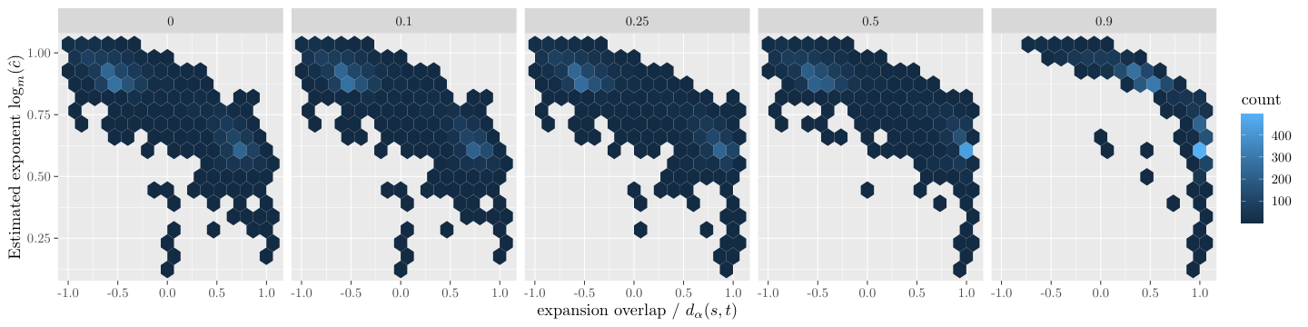
In Fig. 6, we show how the distribution underlying Fig. 3(a) changes if we vary $\alpha$ . It can clearly be seen that the overall relationship between how easily the expansion overlap fulfils the condition of Theorem 3.2 and the estimated exponent remains intact for all values, even though this inflates the length of the cheap prefix $\cheap_{s}$ and suffix $d(s,t)-\cheap_{t}$ . However, this effect only really begins to let apparently linear instances match the condition for sublinear running time for very large values of $\alpha$ like $0.9$ . Contrary for all other depicted values of $\alpha$ the distributions barely change and also the difference between not using the cheap regions at all by setting $\alpha=0$ and using them is not large.

It can also be seen that the arbitrary choice of when to classify instances as linear or sublinear based on their estimated exponent does not matter much. For any of the smaller values of $\alpha$ , the distribution of the graphs is well separated into two clusters of high density, for which the estimated exponent is high, where the condition for Theorem 3.2 is not fulfilled, and significantly lower otherwise.

Similarly, Fig. 7 shows how different values for the minimum base of the expansion $b$ influence the results only slightly as long as $b$ is sufficiently far from $1$ . We again plot the same distribution as above, this time for different values of $b$ between $1$ and $4$ . If $b$ is set to $1$ , then it suffices for two consecutive exploration steps to have non-decreasing cost in order for them to be considered as $b$ -expanding. This increases the lengths of the expansion overlaps slightly, and shifts the plotted distribution to the right, leading to more vertices that fulfil the condition of Theorem 3.2. However it is arguably not very reasonable to expect to observe asymptotic behavior on instances of rather small constant size, if exponential growth is allowed a base too close to $1$ . For only slightly larger bases such as $1.1$ and even more so $2$ and $4$ , the correspondence of theoretical predictions and empirical observations becomes much better. This justifies our choice of $b=2$ and $\alpha=0.1$ in the main part of this paper not just for the sake of simplicity and clarity.